Spectrally-normalized margin bounds for neural networks

Abstract

This paper presents a margin-based multiclass generalization bound for neural networks that scales with their margin-normalized spectral complexity: their Lipschitz constant, meaning the product of the spectral norms of the weight matrices, times a certain correction factor. This bound is empirically investigated for a standard AlexNet network trained with SGD on the mnist and cifar10 datasets, with both original and random labels; the bound, the Lipschitz constants, and the excess risks are all in direct correlation, suggesting both that SGD selects predictors whose complexity scales with the difficulty of the learning task, and secondly that the presented bound is sensitive to this complexity.

1 Overview

Neural networks owe their astonishing success not only to their ability to fit any data set: they also generalize well, meaning they provide a close fit on unseen data. A classical statistical adage is that models capable of fitting too much will generalize poorly; what’s going on here?

Let’s navigate the many possible explanations provided by statistical theory. A first observation is that any analysis based solely on the number of possible labellings on a finite training set — as is the case with VC dimension — is doomed: if the function class can fit all possible labels (as is the case with neural networks in standard configurations (Zhang et al., 2017)), then this analysis can not distinguish it from the collection of all possible functions!

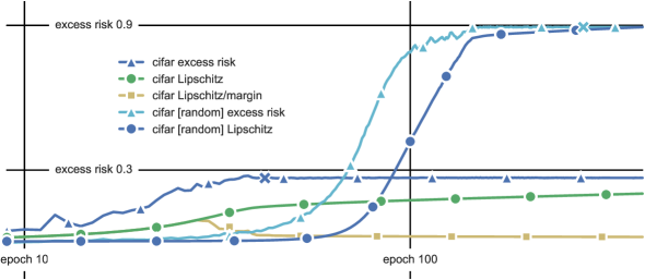
Figure 1: An analysis of AlexNet (Krizhevsky et al., 2012) trained with SGD on cifar10, both with original and with random labels. Triangle-marked curves track excess risk across training epochs (on a log scale), with an ‘x’ marking the earliest epoch with zero training error. Circle-marked curves track Lipschitz constants, normalized so that the two curves for random labels meet. The Lipschitz constants tightly correlate with excess risk, and moreover normalizing them by margins (resulting in the square-marked curve) neutralizes growth across epochs.

Next let’s consider scale-sensitive measures of complexity, such as Rademacher complexity and covering numbers, which (can) work directly with real-valued function classes, and moreover are sensitive to their magnitudes. Figure 1 plots the excess risk (the test error minus the training error) across training epochs against one candidate scale-sensitive complexity measure, the Lipschitz constant of the network (the product of the spectral norms of the weight matrices), and demonstrates that they are tightly correlated (which is not the case for, say, the $l_{2}$ norm of the weights). The data considered in Figure 1 is the standard cifar10 dataset, both with original and with random labels, which has been used as a sanity check when investigating neural network generalization (Zhang et al., 2017).

There is still an issue with basing a complexity measure purely on the Lipschitz constant (although it has already been successfully employed to regularize neural networks (Cisse et al., 2017)): as depicted in Figure 1, the measure grows over time, despite the excess risk plateauing. Fortunately, there is a standard resolution to this issue: investigating the margins (a precise measure of confidence) of the outputs of the network. This tool has been used to study the behavior of 2-layer networks, boosting methods, SVMs, and many others (Bartlett, 1996; Schapire et al., 1997; Boucheron et al., 2005); in boosting, for instance, there is a similar growth in complexity over time (each training iteration adds a weak learner), whereas margin bounds correctly stay flat or even decrease. This behavior is recovered here: as depicted in Figure 1, even though standard networks exhibit growing Lipschitz constants, normalizing these Lipschitz constants by the margin instead gives a decaying curve.

1.1 Contributions

This work investigates a complexity measure for neural networks that is based on the Lipschitz constant, but normalized by the margin of the predictor. The two central contributions are as follows.

• Theorem 1.1 below will give the rigorous statement of the generalization bound that is the basis of this work. In contrast to prior work, this bound: (a) scales with the Lipschitz constant (product of spectral norms of weight matrices) divided by the margin; (b) has no dependence on combinatorial parameters (e.g., number of layers or nodes) outside of log factors; (c) is multiclass (with no explicit dependence on the number of classes); (d) measures complexity against a reference network (e.g., for the ResNet (He et al., 2016), the reference network has identity mappings at each layer). The bound is stated below, with a general form and analysis summary appearing in Section 3 and the full details relegated to the appendix.

• An empirical investigation, in Section 2, of neural network generalization on the standard datasets cifar10, cifar100, and mnist using the preceding bound. Rather than using the bound to provide a single number, it can be used to form a margin distribution as in Figure 2. These margin distributions will illuminate the following intuitive observations: (a) cifar10 is harder than mnist; (b) random labels make cifar10 and mnist much more difficult; (c) the margin distributions (and bounds) converge during training, even though the weight matrices continue to grow; (d) $l_{2}$ regularization (“weight decay”) does not significantly impact margins or generalization.

A more detailed description of the margin distributions is as follows. Suppose a neural network computes a function $f\mathrel{\mathop{\ordinarycolon}}\mathbb{R}^{d}\to\mathbb{R}^{k}$, where $k$ is the number of classes; the most natural way to convert this to a classifier is to select the output coordinate with the largest magnitude, meaning $x\mapsto\operatorname*{arg\,max}_{j}f(x)_{j}$. The margin, then, measures the gap between the output for the correct label and other labels, meaning $f(x)_{y}-\max_{j\neq y}f(x)_{j}$.

Unfortunately, margins alone do not seem to say much; see for instance Figure 2(a), where the collections of all margins for all data points — the unnormalized margin distribution — are similar for cifar10 with and without random labels. What is missing is an appropriate normalization, as in Figure 2(b). This normalization is provided by Theorem 1.1, which can now be explained in detail.

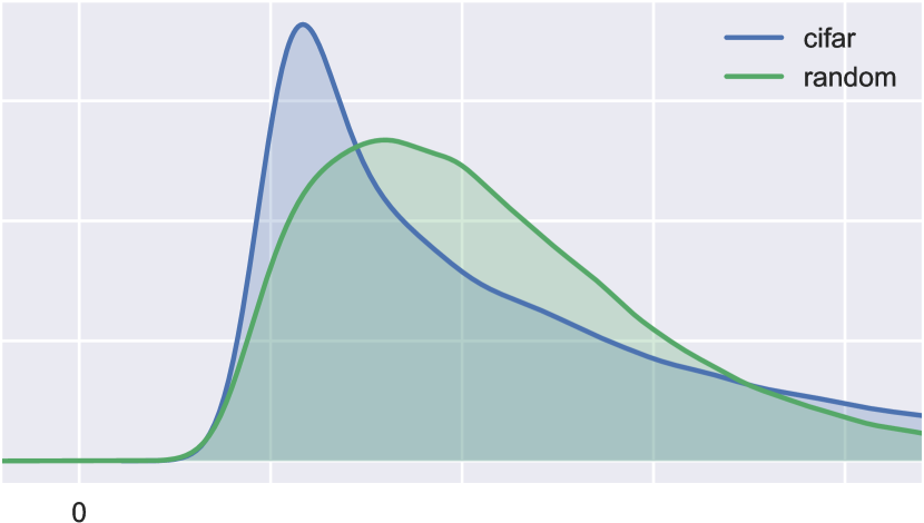
(a) Margins.

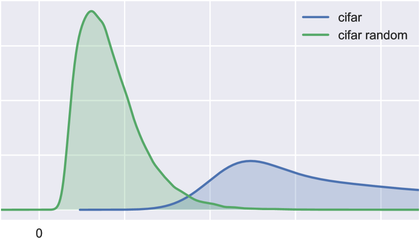
(b) Normalized margins.

Figure 2: Margin distributions at the end of training AlexNet on cifar10, with and without random labels. With proper normalization, random labels demonstrably correspond to a harder problem.

To state the bound, a little bit of notation is necessary. The networks will use $L$ fixed nonlinearities $(\sigma_{1},\ldots,\sigma_{L})$, where $\sigma_{i}\mathrel{\mathop{\ordinarycolon}}\mathbb{R}^{d_{i-1}}\to\mathbb{R}^{d_{i}}$ is $\rho_{i}$-Lipschitz (e.g., as with coordinate-wise ReLU, and max-pooling, as discussed in Section A.1); occasionally, it will also hold that $\sigma_{i}(0)=0$. Given $L$ weight matrices $\mathcal{A}=(A_{1},\ldots,A_{L})$ let $F_{\mathcal{A}}$ denote the function computed by the corresponding network:

$$F_{\mathcal{A}}(x)\mathrel{\mathop{\ordinarycolon}}=\sigma_{L}(A_{L}\sigma_{L-1}(A_{L-1}\cdots\sigma_{1}(A_{1}x)\cdots)).$$ (1.1)

The network output $F_{\mathcal{A}}(x)\in\mathbb{R}^{d_{L}}$ (with $d_{0}=d$ and $d_{L}=k$) is converted to a class label in $\{1,\ldots,k\}$ by taking the $\arg\max$ over components, with an arbitrary rule for breaking ties. Whenever input data $x_{1},\ldots,x_{n}\in\mathbb{R}^{d}$ are given, collect them as rows of a matrix $X\in\mathbb{R}^{n\times d}$. Occasionally, notation will be overloaded to discuss $F_{\mathcal{A}}(X^{T})$, a matrix whose $i^{\textup{th}}$ column is $F_{\mathcal{A}}(x_{i})$. Let $W$ denote the maximum of $\{d,d_{1},\ldots,d_{L}\}$. The $l_{2}$ norm $\|\cdot\|_{2}$ is always computed entry-wise; thus, for a matrix, it corresponds to the Frobenius norm.

Next, define a collection of reference matrices $(M_{1},\ldots,M_{L})$ with the same dimensions as $A_{1},\ldots,A_{L}$; for instance, to obtain a good bound for ResNet (He et al., 2016), it is sensible to set $M_{i}\mathrel{\mathop{\ordinarycolon}}=I$, the identity map, and the bound below will worsen as the network moves farther from the identity map; for AlexNet (Krizhevsky et al., 2012), the simple choice $M_{i}=0$ suffices. Finally, let $\|\cdot\|_{\sigma}$ denote the spectral norm, and let $\|\cdot\|_{p,q}$ denote the $(p,q)$ matrix norm, defined by $\left\|A\right\|_{p,q}\mathrel{\mathop{\ordinarycolon}}=\mathinner{\!\left\lVert(\|{}A_{\mathrel{\mathop{\ordinarycolon}},1}\|_{p},\ldots,\|{}A_{\mathrel{\mathop{\ordinarycolon}},m}\|_{p})\right\rVert}_{q}$ for $A\in\mathbb{R}^{d\times{}m}$. The spectral complexity $R_{F_{\mathcal{A}}}=R_{\mathcal{A}}$ of a network $F_{\mathcal{A}}$ with weights $\mathcal{A}$ is the defined as

$$R_{\mathcal{A}}\mathrel{\mathop{\ordinarycolon}}=\mathinner{\left(\prod_{i=1}^{L}\rho_{i}\|A_{i}\|_{\sigma}\right)}\mathinner{\left(\sum_{i=1}^{L}\frac{\|A_{i}^{\top}-M_{i}^{\top}\|_{2,1}^{2/3}}{\|A_{i}\|_{\sigma}^{2/3}}\right)}^{3/2}.$$ (1.2)

The following theorem provides a generalization bound for neural networks whose nonlinearities are fixed but whose weight matrices $\mathcal{A}$ have bounded spectral complexity $R_{\mathcal{A}}$.

Theorem 1.1.

Let nonlinearities $(\sigma_{1},\ldots,\sigma_{L})$ and reference matrices $(M_{1},\ldots,M_{L})$ be given as above (i.e., $\sigma_{i}$ is $\rho_{i}$-Lipschitz and $\sigma_{i}(0)=0$). Then for $(x,y),(x_{1},y_{1}),\ldots,(x_{n},y_{n})$ drawn iid from any probability distribution over $\mathbb{R}^{d}\times\{1,\ldots,k\}$, with probability at least $1-\delta$ over $((x_{i},y_{i}))_{i=1}^{n}$, every margin $\gamma>0$ and network $F_{\mathcal{A}}\mathrel{\mathop{\ordinarycolon}}\mathbb{R}^{d}\to\mathbb{R}^{k}$ with weight matrices $\mathcal{A}=(A_{1},\ldots,A_{L})$ satisfy

$$\textup{Pr}\mathinner{\Bigl{[}\operatorname*{arg\,max}_{j}F_{\mathcal{A}}(x)_{j}\neq y\Bigr{]}}\leq\widehat{\mathcal{R}}_{\gamma}(F_{\mathcal{A}})+\widetilde{\mathcal{O}}\mathinner{\left(\frac{\|X\|_{2}R_{\mathcal{A}}}{\gamma n}\ln(W)+\sqrt{\frac{\ln(1/\delta)}{n}}\right)},$$

where $\widehat{\mathcal{R}}_{\gamma}(f)\leq n^{-1}\sum_{i}\mathds{1}\mathinner{\left[f(x_{i})_{y_{i}}\leq\gamma+\max_{j\neq y_{i}}f(x_{i})_{j}\right]}$ and $\|X\|_{2}=\sqrt{\sum_{i}\|x_{i}\|_{2}^{2}}$.

The full proof and a generalization beyond spectral norms is relegated to the appendix, but a sketch is provided in Section 3, along with a lower bound. Section 3 also gives a discussion of related work: briefly, it’s essential to note that margin and Lipschitz-sensitive bounds have a long history in the neural networks literature (Bartlett, 1996; Anthony and Bartlett, 1999; Neyshabur et al., 2015); the distinction here is the sensitivity to the spectral norm, and that there is no explicit appearance of combinatorial quantities such as numbers of parameters or layers (outside of log terms, and indices to summations and products).

To close, miscellaneous observations and open problems are collected in Section 4.

2 Generalization case studies via margin distributions

In this section, we empirically study the generalization behavior of neural networks, via margin distributions and the generalization bound stated in Theorem 1.1.

Before proceeding with the plots, it’s a good time to give a more refined description of the margin distribution, one that is suitable for comparisons across datasets. Given $n$ pattern/label pairs $((x_{i},y_{i}))_{i=1}^{n}$, with patterns as rows of matrix $X\in\mathbb{R}^{n\times d}$, and given a predictor $F_{\mathcal{A}}\mathrel{\mathop{\ordinarycolon}}\mathbb{R}^{d}\to\mathbb{R}^{k}$, the (normalized) margin distribution is the univariate empirical distribution of the labeled data points each transformed into a single scalar according to

$$(x,y)\mapsto\frac{F_{\mathcal{A}}(x)_{y}-\max_{i\neq y}F_{\mathcal{A}}(x)_{i}}{R_{\mathcal{A}}\|X\|_{2}/n},$$

where the spectral complexity $R_{\mathcal{A}}$ is from eq. 1.2. The normalization is thus derived from the bound in Theorem 1.1, but ignoring log terms.

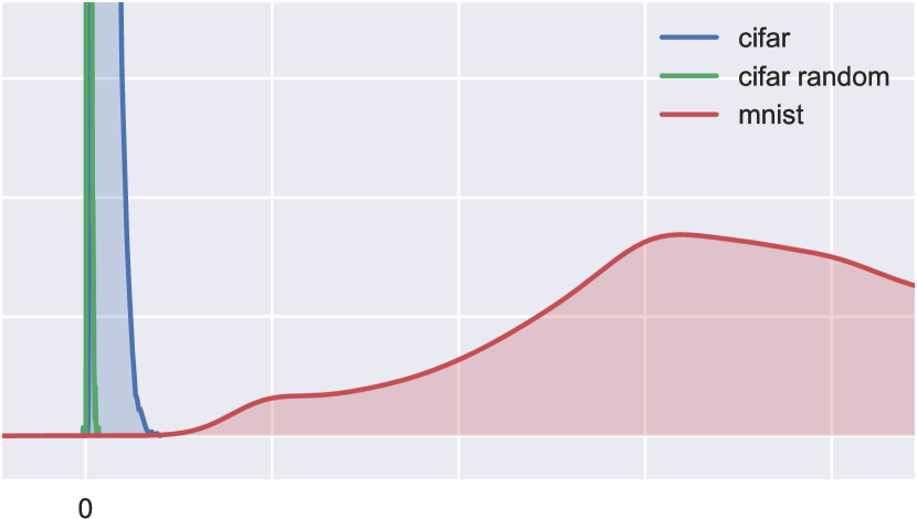
(a) mnist is easier than cifar10.

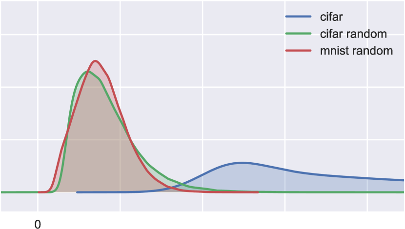
(b) Random mnist is as hard as random cifar10!

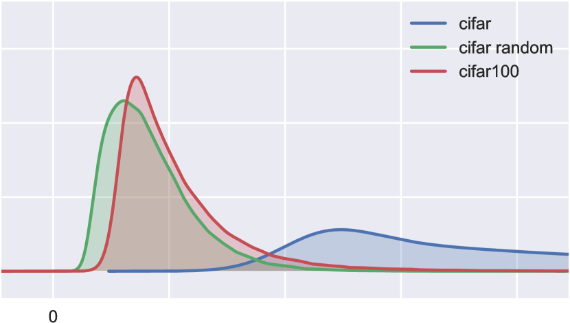
(c) cifar100 is as hard as cifar10 with random labels!

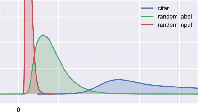
(d) Random inputs are harder than random labels.

Figure 3: A variety of margin distributions. Axes are re-scaled in Figure 3(a), but identical in the other subplots; the cifar10 (blue) and random cifar10 (green) distributions are the same each time.

Taken this way, the two margin distributions for two datasets can be interpreted as follows. Considering any fixed point on the horizontal axis, if the cumulative distribution of one density is lower than the other, then it corresponds to a lower right hand side in Theorem 1.1. For no reason other than visual interpretability, the plots here will instead depict a density estimate of the margin distribution. The vertical and horizontal axes are rescaled in different plots, but the random and true cifar10 margin distributions are always the same.

A little more detail about the experimental setup is as follows. All experiments were implemented in Keras (Chollet et al., 2015). In order to minimize conflating effects of optimization and regularization, the optimization method was vanilla SGD with step size $0.01$, and all regularization (weight decay, batch normalization, etc.) were disabled. “cifar” in general refers to cifar10, however cifar100 will also be explicitly mentioned. The network architecture is essentially AlexNet (Krizhevsky et al., 2012) with all normalization/regularization removed, and with no adjustments of any kind (even to the learning rate) across the different experiments.

Comparing datasets. A first comparison is of cifar10 and the standard mnist digit data. mnist is considered “easy”, since any of a variety of methods can achieve roughly 1% test error. The “easiness” is corroborated by Figure 3(a), where the margin distribution for mnist places all its mass far to the right of the mass for cifar10. Interestingly, randomizing the labels of mnist, as in Figure 3(b), results in a margin distribution to the left of not only cifar10, but also slightly to the left of (but close to) cifar10 with randomized labels.

Next, Figure 3(c) compares cifar10 and cifar100, where cifar100 uses the same input images as cifar10; indeed, cifar10 is obtained from cifar100 by collapsing the original 100 categories into 10 groups. Interestingly, cifar100, from the perspective of margin bounds, is just as difficult as cifar10 with random labels. This is consistent with the large observed test error on cifar100 (which has not been “optimized” in any way via regularization).

Lastly, Figure 3(d) replaces the cifar10 input images with random images sampled from Gaussians matching the first- and second-order image statistics (see (Zhang et al., 2017) for similar experiments).

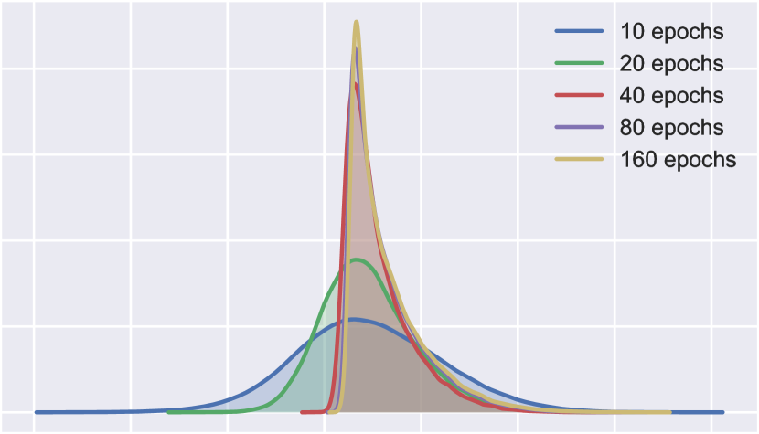
(a) Margins across epochs for cifar10.

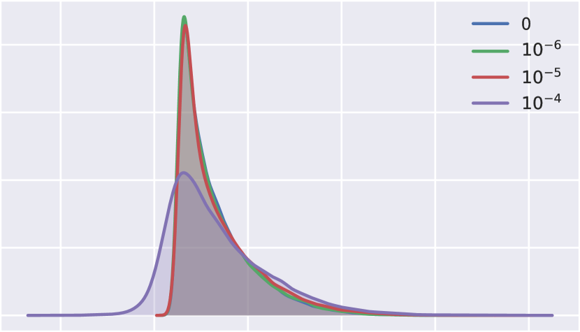
(b) Various levels of $l_{2}$ regularization for cifar10.

Figure 4:

Convergence of margins. As was pointed out in Section 1, the weights of the neural networks do not seem to converge in the usual sense during training (the norms grow continually). However, as depicted in Figure 4(a), the sequence of (normalized) margin distributions is itself converging.

Regularization. As remarked in (Zhang et al., 2017), regularization only seems to bring minor benefits to test error (though adequate to be employed in all cutting edge results). This observation is certainly consistent with the margin distributions in Figure 4(b), which do not improve (e.g., by shifting to the right) in any visible way under regularization. An open question, discussed further in Section 4, is to design regularization that improves margins.

3 Analysis of margin bound

This section will sketch the proof of Theorem 1.1, give a lower bound, and discuss related work.

3.1 Multiclass margin bound

The starting point of this analysis is a margin-based bound for multiclass prediction. To state the bound, first recall that the margin operator $\mathcal{M}\mathrel{\mathop{\ordinarycolon}}\mathbb{R}^{k}\times\{1,\ldots,k\}\to\mathbb{R}$ is defined as $\displaystyle\mathcal{M}(v,y)\mathrel{\mathop{\ordinarycolon}}=v_{y}-\max_{i\neq y}v_{i}$, and define the ramp loss $\ell_{\gamma}\mathrel{\mathop{\ordinarycolon}}\mathbb{R}\to\mathbb{R}^{+}$ as

$$\ell_{\gamma}(r)\mathrel{\mathop{\ordinarycolon}}=\begin{cases}0&r<-\gamma,\\ 1+r/\gamma&r\in[-\gamma,0],\\ 1&r>0,\end{cases}$$

and ramp risk as $\displaystyle\mathcal{R}_{\gamma}(f)\mathrel{\mathop{\ordinarycolon}}=\mathbb{E}(\ell_{\gamma}(-\mathcal{M}(f(x),y)))$. Given a sample $S\mathrel{\mathop{\ordinarycolon}}=((x_{1},y_{1}),\ldots,(x_{n},y_{n}))$, define an empirical counterpart $\widehat{\mathcal{R}}_{\gamma}$ of $\mathcal{R}_{\gamma}$ as $\widehat{\mathcal{R}}_{\gamma}(f)\mathrel{\mathop{\ordinarycolon}}=n^{-1}\sum_{i}\ell_{\gamma}(-\mathcal{M}(f(x_{i}),y_{i}))$; note that $\mathcal{R}_{\gamma}$ and $\widehat{\mathcal{R}}_{\gamma}$ respectively upper bound the probability and fraction of errors on the source distribution and training set. Lastly, given a set of real-valued functions $\mathcal{H}$, define the Rademacher complexity as $\mathfrak{R}(\mathcal{H}_{|S})\mathrel{\mathop{\ordinarycolon}}=n^{-1}\mathbb{E}\sup_{h\in\mathcal{H}}\sum_{i=1}^{n}\epsilon_{i}h(x_{i},y_{i})$, where the expectation is over the Rademacher random variables $(\epsilon_{1},\ldots,\epsilon_{n})$, which are iid with $\textup{Pr}[\epsilon_{1}=1]=\textup{Pr}[\epsilon_{1}=-1]=\nicefrac{{1}}{{2}}$.

With this notation in place, the basic bound is as follows.

Lemma 3.1.

Given functions $\mathcal{F}$ with $\mathcal{F}\ni f\mathrel{\mathop{\ordinarycolon}}\mathbb{R}^{d}\to\mathbb{R}^{k}$ and any $\gamma>0$, define

$$\mathcal{F}_{\gamma}\mathrel{\mathop{\ordinarycolon}}=\mathinner{\left\{(x,y)\mapsto\ell_{\gamma}(-\mathcal{M}(f(x),y))\mathrel{\mathop{\ordinarycolon}}f\in\mathcal{F}\right\}}.$$

Then, with probability at least $1-\delta$ over a sample $S$ of size $n$, every $f\in\mathcal{F}$ satisfies

$$\textup{Pr}[\operatorname*{arg\,max}_{i}f(x)_{i}\neq y]\leq\widehat{\mathcal{R}}_{\gamma}(f)+2\mathfrak{R}((\mathcal{F}_{\gamma})_{|S})+3\sqrt{\frac{\ln(1/\delta)}{2n}}.$$

This bound is a direct consequence of standard tools in Rademacher complexity. In order to instantiate this bound, covering numbers will be used to directly upper bound the Rademacher complexity term $\mathfrak{R}((\mathcal{F}_{\gamma})_{|S})$. Interestingly, the choice of directly working in terms of covering numbers seems essential to providing a bound with no explicit dependence on $k$; by contrast, prior work primarily handles multiclass via a Rademacher complexity analysis on each coordinate of a $k$-tuple of functions, and pays a factor of $\sqrt{k}$ (Zhang, 2004).

3.2 Covering number complexity upper bounds

This subsection proves Theorem 1.1 via Lemma 3.1 by controlling, via covering numbers, the Rademacher complexity $\mathfrak{R}((\mathcal{F}_{\gamma})_{|S})$ for networks with bounded spectral complexity.

The notation here for (proper) covering numbers is as follows. Let $\mathcal{N}(U,\epsilon,\|\cdot\|)$ denote the least cardinality of any subset $V\subseteq U$ that covers $U$ at scale $\epsilon$ with norm $\|\cdot\|$, meaning

$$\sup_{A\in U}\min_{B\in V}\|A-B\|\leq\epsilon.$$

Choices of $U$ that will be used in the present work include both the image $\mathcal{F}_{|S}$ of data $S$ under some function class $\mathcal{F}$, as well as the conceptually simpler choice of a family of matrix products.

The full proof has the following steps. (I) A matrix covering bound for the affine transformation of each layer is provided in Lemma 3.2; handling whole layers at once allows for more flexible norms. (II) An induction on layers then gives a covering number bound for entire networks; this analysis is only sketched here for the special case of norms used in Theorem 1.1, but the full proof in the appendix culminates in a bound for more general norms (cf. Lemma A.7). (III) The preceding whole-network covering number leads to Theorem 1.1 via Lemma 3.1 and standard techniques.

Step (I), matrix covering, is handled by the following lemma. The covering number considers the matrix product $XA$, where $A$ will be instantiated as the weight matrix for a layer, and $X$ is the data passed through all layers prior to the present layer.

Lemma 3.2.

Let conjugate exponents $(p,q)$ and $(r,s)$ be given with $p\leq 2$, as well as positive reals $(a,b,\epsilon)$ and positive integer $m$. Let matrix $X\in\mathbb{R}^{n\times d}$ be given with $\|X\|_{p}\leq b$. Then

$$\ln\mathcal{N}\mathinner{\left(\mathinner{\left\{XA\mathrel{\mathop{\ordinarycolon}}A\in\mathbb{R}^{d\times m},\|A\|_{q,s}\leq a\right\}},\epsilon,\|\cdot\|_{2}\right)}\leq\left\lceil\frac{a^{2}b^{2}m^{2/r}}{\epsilon^{2}}\right\rceil\ln(2dm).$$

The proof relies upon the Maurey sparsification lemma (Pisier, 1980), which is stated in terms of sparsifying convex hulls, and in its use here is inspired by covering number bounds for linear predictors (Zhang, 2002). To prove Theorem 1.1, this matrix covering bound will be instantiated for the case of $\left\|A\right\|_{2,1}$. It is possible to instead scale with $\|A\|_{2}$ and $\|X\|_{2}$, but even for the case of the identity matrix $X=I$, this incurs an extra dimension factor. The use of $\|A\|_{2,1}$ here thus helps Theorem 1.1 avoid any appearance of $W$ and $L$ outside of log terms; indeed, the goal of covering a whole matrix at a time (rather than the more standard vector covering) was to allow this greater sensitivity and avoid combinatorial parameters.

Step (II), the induction on layers, proceeds as follows. Let $X_{i}$ denote the output of layer $i$ but with images of examples of columns (thus $X_{0}=X^{\top}$), and inductively suppose there exists a cover element $\widehat{X}_{i}$ for $X_{i}$ which depends on covering matrices $(\widehat{A}_{1},\ldots,\widehat{A}_{i-1})$ chosen to cover weight matrices in earlier layers. Thanks to Lemma 3.2, there also exists $\widehat{A}_{i}$ so that $\|A_{i}\widehat{X}_{i}-\widehat{A}_{i}\widehat{X}_{i}\|_{2}\leq\epsilon_{i}$. The desired cover element is thus $\widehat{X}_{i+1}=\sigma_{i}(\widehat{A}_{i}\widehat{X}_{i})$ where $\sigma_{i}$ is the nonlinearity in layer $i$; indeed, supposing $\sigma_{i}$ is $\rho_{i}$-Lipschitz,

$$\|X_{i+1}-\widehat{X}_{i+1}\|_{2} \leq\rho_{i}\|A_{i}X_{i}-\widehat{A}_{i}\widehat{X}_{i}\|_{2}$$

$$\leq\rho_{i}\mathinner{\left(\|A_{i}X_{i}-A_{i}\widehat{X}_{i}\|_{2}+\|A_{i}\widehat{X}_{i}-\widehat{A}_{i}\widehat{X}_{i}\|_{2}\right)}$$

$$\leq\rho_{i}\|A_{i}\|_{\sigma}\|X_{i}-\widehat{X}_{i}\|_{2}+\rho_{i}\epsilon_{i},$$

where the first term is controlled with the inductive hypothesis. Since $\widehat{X}_{i+1}$ depends on each choice $(\widehat{A}_{i},\ldots,\widehat{A}_{i})$, the cardinality of the full network cover is the product of the individual matrix covers.

The preceding proof had no sensitivity to the particular choice of norms; it merely required an operator norm on $A_{i}$, as well as some other norm that allows matrix covering. Such an analysis is presented in full generality in Section A.5. Specializing to the particular case of spectral norms and $(2,1)$ group norms leads to the following full-network covering bound.

Theorem 3.3.

Let fixed nonlinearities $(\sigma_{1},\ldots,\sigma_{L})$ and reference matrices $(M_{1},\ldots,M_{L})$ be given, where $\sigma_{i}$ is $\rho_{i}$-Lipschitz and $\sigma_{i}(0)=0$. Let spectral norm bounds $(s_{1},\ldots,s_{L})$, and matrix $(2,1)$ norm bounds $(b_{1},\ldots,b_{L})$ be given. Let data matrix $X\in\mathbb{R}^{n\times d}$ be given, where the $n$ rows correspond to data points. Let $\mathcal{H}_{X}$ denote the family of matrices obtained by evaluating $X$ with all choices of network $F_{\mathcal{A}}$:

$$\mathcal{H}_{X}\mathrel{\mathop{\ordinarycolon}}=\mathinner{\left\{F_{\mathcal{A}}(X^{T})\ \mathrel{\mathop{\ordinarycolon}}\ \mathcal{A}=(A_{1},\ldots,A_{L}),\ \|A_{i}\|_{\sigma}\leq s_{i},\ \|A_{i}^{\top}-M_{i}^{\top}\|_{2,1}\leq b_{i}\right\}},$$

where each matrix has dimension at most $W$ along each axis. Then for any $\epsilon>0$,

$$\ln\mathcal{N}(\mathcal{H}_{X},\epsilon,\|\cdot\|_{2})\leq\frac{\|X\|^{2}_{2}\ln(2W^{2})}{\epsilon^{2}}\mathinner{\left(\prod_{j=1}^{L}s_{j}^{2}\rho_{j}^{2}\right)}\mathinner{\left(\sum_{i=1}^{L}\mathinner{\left(\frac{b_{i}}{s_{i}}\right)}^{2/3}\right)}^{3}.$$

What remains is (III): Theorem 3.3 can be combined with the standard Dudley entropy integral upper bound on Rademacher complexity (see e.g. Mohri et al. (2012)), which together with Lemma 3.1 gives Theorem 1.1.

3.3 Rademacher complexity lower bounds

By reduction to the linear case (i.e., removing all nonlinearities), it is easy to provide a lower bound on the Rademacher complexity of the networks studied here. Unfortunately, this bound only scales with the product of spectral norms, and not the other terms in $R_{\mathcal{A}}$ (cf. eq. 1.2).

Theorem 3.4.

Consider the setting of Theorem 3.3, but all nonlinearities are the ReLU $z\mapsto\max\{0,z\}$, the output dimension is $d_{L}=1$, and all non-output dimensions are at least 2 (and hence $W\geq 2$). Let data $S\mathrel{\mathop{\ordinarycolon}}=(x_{1},\ldots,x_{n})$ be collected into data matrix $X\in\mathbb{R}^{n\times d}$. Then there is a $c$ such that for any scalar $r>0$,

$$\mathfrak{R}\mathinner{\biggl{(}\mathinner{\Bigl{\{}F_{\mathcal{A}}\mathrel{\mathop{\ordinarycolon}}\mathcal{A}=(A_{1},\ldots,A_{L}),\ \prod_{i}\|A_{i}\|_{\sigma}\leq r\Bigr{\}}}_{|S}\biggr{)}}\geq c\left\|X\right\|_{2}r.$$ (3.1)

Note that, due to the nonlinearity, the lower bound should indeed depend on $\prod_{i}\|A_{i}\|_{\sigma}$ and not $\|\prod_{i}A_{i}\|_{\sigma}$; as a simple sanity check, there exist networks for which the latter quantity is 0, but the network does not compute the zero function.

3.4 Related work

To close this section on proofs, it is a good time to summarize connections to existing literature.

The algorithmic idea of large margin classifiers was introduced in the linear case by Vapnik (1982) (see also (Boser et al., 1992; Cortes and Vapnik, 1995)). Vapnik (1995) gave an intuitive explanation of the performance of these methods based on a sample-dependent VC-dimension calculation, but without generalization bounds. The first rigorous generalization bounds for large margin linear classifiers (Shawe-Taylor et al., 1998) required a scale-sensitive complexity analysis of real-valued function classes. At the same time, a large margin analysis was developed for two-layer networks (Bartlett, 1996), indeed with a proof technique that inspired the layer-wise induction used to prove Theorem 1.1 in the present work. Margin theory was quickly extended to many other settings (see for instance the survey by Boucheron et al. (2005)), one major success being an explanation of the generalization ability of boosting methods, which exhibit an explicit growth in the size of the function class over time, but a stable excess risk (Schapire et al., 1997). The contribution of the present work is to provide a margin bound (and corresponding Rademacher analysis) that can be adapted to various operator norms at each layer. Additionally, the present work operates in the multiclass setting, and avoids an explicit dependence on the number of classes $k$, which seems to appear in prior work (Zhang, 2004; Tewari and Bartlett, 2007).

There are numerous generalization bounds for neural networks, including VC-dimension and fat-shattering bounds (many of these can be found in (Anthony and Bartlett, 1999)). Scale-sensitive analysis of neural networks started with (Bartlett, 1996), which can be interpreted in the present setting as utilizing data norm $\|\cdot\|_{\infty}$ and operator norm $\|\cdot\|_{\infty\to\infty}$ (equivalently, the norm $\|A_{i}^{\top}\|_{1,\infty}$ on weight matrix $A_{i}$). This analysis can be adapted to give a Rademacher complexity analysis (Bartlett and Mendelson, 2002), and has been adapted to other norms (Neyshabur et al., 2015), although the $\|\cdot\|_{\infty}$ setting appears to be necessary to avoid extra combinatorial factors. More work is still needed to develop complexity analyses that have matching upper and lower bounds, and also to determine which norms are well-adapted to neural networks as used in practice.

The present analysis utilizes covering numbers, and is most closely connected to earlier covering number bounds (Anthony and Bartlett, 1999, Chapter 12), themselves based on the earlier fat-shattering analysis (Bartlett, 1996), however the technique here of pushing an empirical cover through layers is akin to VC dimension proofs for neural networks (Anthony and Bartlett, 1999). The use of Maurey’s sparsification lemma was inspired by linear predictor covering number bounds (Zhang, 2002).

Comparison to preprint. The original preprint of this paper (Bartlett et al., 2017) featured a slightly different version of the spectral complexity $R_{\mathcal{A}}$, given by $\mathinner{\left(\prod_{i=1}^{L}\rho_{i}\|A_{i}\|_{\sigma}\right)}\mathinner{\left(\sum_{i=1}^{L}\frac{\|A_{i}-M_{i}\|_{1}^{2/3}}{\|A_{i}\|_{\sigma}^{2/3}}\right)}^{3/2}.$ In the present version (1.2), each $\|A_{i}-M_{i}\|_{1}$ term is replaced by $\|A_{i}^{\top}-M_{i}^{\top}\|_{2,1}$. This is a strict improvement since for any matrix $A\in\mathbb{R}^{d\times{}m}$ one has $\left\|A\right\|_{2,1}\leq{}\left\|A\right\|_{1}$, and in general the gap between these two norms can be as large as $\sqrt{d}$.

On a related note, all of the figures in this paper use the $\ell_{1}$ norm in the spectral complexity $R_{\mathcal{A}}$ instead of the $(2,1)$ norm. Variants of the experiments described in Section 2 were carried out using each of the $l_{1}$, $(2,1)$, and $l_{2}$ norms in the $(\sum_{i=1}^{L}(\cdot)^{2/3})^{3/2}$ term with negligible difference in the results.

Since spectrally-normalized margin bounds were first proposed in the preprint (Bartlett et al., 2017), subsequent works (Neyshabur et al., 2017; Neyshabur, 2017) re-derived a similar spectrally-normalized bound using the PAC-Bayes framework. Specifically, these works showed that $R_{\mathcal{A}}$ may be replaced (up to $\ln(W)$ factors) by: $\mathinner{\bigl{(}\prod_{i=1}^{L}\rho_{i}\|A_{i}\|_{\sigma}\bigr{)}}\cdot L\mathinner{\bigl{(}\sum_{i=1}^{L}\frac{(\sqrt{W}\|A_{i}-M_{i}\|_{2})^{2}}{\|A_{i}\|_{\sigma}^{2}}\bigr{)}}^{1/2}$. Unfortunately, this bound never improves on Theorem 1.1, and indeed can be derived from it as follows. First, the dependence on the individual matrices $A_{i}$ in the second term of this bound can be obtained from Theorem 1.1 since for any $A\in\mathbb{R}^{d\times{}m}$ it holds that $\left\|A^{\top}\right\|_{2,1}\leq{}\sqrt{d}\left\|A\right\|_{2}$. Second, the functional form $(\sum_{i=1}^{L}(\cdot)^{2/3})^{3/2}$ appearing in Theorem 1.1 may be replaced by the form $L(\sum_{i=1}^{L}(\cdot)^{2})^{1/2}$ appearing above by using $\left\|\alpha\right\|_{2/3}\leq{}L\left\|\alpha\right\|_{2}$ which holds for any $\alpha\in\mathbb{R}^{L}$ (and can be proved, for instance, with Jensen’s inequality).

4 Further observations and open problems

Adversarial examples.

Adversarial examples are a phenomenon where the neural network predictions can be altered by adding seemingly imperceptible noise to an input (Goodfellow et al., 2014). This phenomenon can be connected to margins as follows. The margin is nothing more than the distance an input must traverse before its label is flipped; consequently, low margin points are more susceptible to adversarial noise than high margin points. Concretely, taking the 100 lowest margin inputs from cifar10 and adding uniform noise at scale $0.15$ yielded flipped labels on 5.86% of the images, whereas the same level of noise on high margin points yielded 0.04% flipped labels. Can the bounds here suggest a way to defend against adversarial examples?

Regularization.

It was observed in (Zhang et al., 2017) that explicit regularization contributes little to the generalization performance of neural networks. In the margin framework, standard weight decay ($l_{2}$) regularization seemed to have little impact on margin distributions in Section 2. On the other hand, in the boosting literature, special types of regularization were developed to maximize margins (Shalev-Shwartz and Singer, 2008); perhaps a similar development can be performed here?

SGD.

The present analysis applies to predictors that have large margins; what is missing is an analysis verifying that SGD applied to standard neural networks returns large margin predictors! Indeed, perhaps SGD returns not simply large margin predictors, but predictors that are well-behaved in a variety of other ways that can be directly translated into refined generalization bounds.

Improvements to Theorem 1.1.

There are several directions in which Theorem 1.1 might be improved. Can a better choice of layer geometries (norms) yield better bounds on practical networks? Can the nonlinearities’ worst-case Lipschitz constant be replaced with an (empirically) averaged quantity? Alternatively, can better lower bounds rule out these directions?

Rademacher vs. covering.

Is it possible to prove Theorem 1.1 solely via Rademacher complexity, with no invocation of covering numbers?

Acknowledgements

The authors thank Srinadh Bhojanapalli, Ryan Jian, Behnam Neyshabur, Maxim Raginsky, Andrew J. Risteski, and Belinda Tzen for useful conversations and feedback. The authors thank Ben Recht for giving a provocative lecture at the Simons Institute, stressing the need for understanding of both generalization and optimization of neural networks. M.T. and D.F. acknowledge the use of a GPU machine provided by Karthik Sridharan and made possible by an NVIDIA GPU grant. D.F. acknowledges the support of the NDSEG fellowship. P.B. gratefully acknowledges the support of the NSF through grant IIS-1619362 and of the Australian Research Council through an Australian Laureate Fellowship (FL110100281) and through the ARC Centre of Excellence for Mathematical and Statistical Frontiers. The authors thank the Simons Institute for the Theory of Computing Spring 2017 program on the Foundations of Machine Learning. Lastly, the authors are grateful to La Burrita (both the north and the south Berkeley campus locations) for upholding the glorious tradition of the California Burrito.

Appendix A Proofs

This appendix collects various proofs omitted from the main text.

A.1 Lipschitz properties of ReLU and max-pooling nonlinearities

The standard ReLU (“Rectified Linear Unit”) is the univariate mapping

$$\sigma_{\textup{r}}(r)\mathrel{\mathop{\ordinarycolon}}=\max\{0,r\}.$$

When applied to a vector or a matrix, it operates coordinate-wise. While the ReLU is currently the most popular choice of univariate nonlinearity, another common choice is the sigmoid $r\mapsto 1/(1+\exp(-r))$. More generally, these univariate nonlinearities are Lipschitz, and this carries over to their vector and matrix forms as follows.

Lemma A.1.

If $\sigma\mathrel{\mathop{\ordinarycolon}}\mathbb{R}^{d}\to\mathbb{R}^{d}$ is $\rho$-Lipschitz along every coordinate, then it is $\rho$-Lipschitz according to $\|\cdot\|_{p}$ for any $p\geq 1$.

Proof.

for any $z,z^{\prime}\in\mathbb{R}^{d}$,

$$\|\sigma(z)-\sigma(z^{\prime})\|_{p}=\mathinner{\left(\sum_{i}|\sigma(z)_{i}-\sigma(z^{\prime})_{i}|^{p}\right)}^{1/p}\leq\mathinner{\left(\sum_{i}\rho^{p}|z_{i}-z^{\prime}_{i}|^{p}\right)}^{1/p}=\rho\|z-z^{\prime}\|_{p}.$$

∎

Define a max-pooling operator $\mathcal{P}$ as follows. Given an input and output pair of finite-dimensional vector spaces $\mathcal{T}$ and $\mathcal{T}^{\prime}$ (possibly arranged as matrices or tensors), the max-pooling operator iterates over a collection of sets of indices $\mathcal{Z}$ (whose cardinality is equal to the dimension of $\mathcal{T}$’), and for each element of $Z_{i}\in\mathcal{Z}$ sets the corresponding coordinate $i$ in the output to the maximum entry of the input over $Z_{i}$: given $T\in\mathcal{T}$,

$$\mathcal{P}(T)_{i}\mathrel{\mathop{\ordinarycolon}}=\max_{j\in Z_{i}}T_{j}.$$

The following Lipschitz constant of pooling operators will depend on the number of times each coordinate is accessed across elements of $\mathcal{Z}$; when this operator is used in computer vision, the number of times is typically a small constant, for instance 5 or 9 (Krizhevsky et al., 2012).

Lemma A.2.

Suppose that each coordinate $j$ of the input appears in at most $m$ elements of the collection $\mathcal{Z}$. Then the max-pooling operator $\mathcal{P}$ is $m^{1/p}$-Lipschitz wrt $\|\cdot\|_{p}$ for any $p\geq 1$. In particular, the max-pooling operator is $1$-Lipschitz whenever $\mathcal{Z}$ forms a partition.

Proof.

Let $T,T^{\prime}\in\mathcal{T}$ be given. First consider any fixed set of indices $Z\in\mathcal{Z}$, and suppose without loss of generality that $\mathcal{P}(T)_{Z}=\max_{j\in Z}T_{j}\geq\max_{j\in Z}T^{\prime}_{j}$. Then

$$|\mathcal{P}(T)_{Z}-\mathcal{P}(T^{\prime})_{Z}|^{p}=\mathinner{\left(\min_{j^{\prime}\in Z}\max_{j\in Z}T_{j}-T^{\prime}_{j^{\prime}}\right)}^{p}\leq\max_{j\in Z}\mathinner{\left(T_{j}-T^{\prime}_{j}\right)}^{p}\leq\sum_{j\in Z}\mathinner{\!\left\lvert T_{j}-T^{\prime}_{j}\right\rvert}^{p}.$$

Consequently,

$$\|\mathcal{P}(T)-\mathcal{P}(T^{\prime})\|_{p} =\mathinner{\left(\sum_{i}|\mathcal{P}(T)_{i}-\mathcal{P}(T^{\prime})_{i}|^{p}\right)}^{1/p}=\mathinner{\left(\sum_{Z\in\mathcal{Z}}|\mathcal{P}(T)_{Z}-\mathcal{P}(T^{\prime})_{Z}|^{p}\right)}^{1/p}$$

$$\leq\mathinner{\left(\sum_{Z\in\mathcal{Z}}\sum_{j\in Z}|T_{j}-T^{\prime}_{j}|^{p}\right)}^{1/p}=\mathinner{\left(\sum_{j}\sum_{Z\in\mathcal{Z}\mathrel{\mathop{\ordinarycolon}}j\in{}Z}|T_{j}-T^{\prime}_{j}|^{p}\right)}^{1/p}$$

$$\leq{}\mathinner{\left(m\sum_{j}|T_{j}-T^{\prime}_{j}|^{p}\right)}^{1/p}=m^{1/p}\|T-T^{\prime}\|_{p}.$$

∎

A.2 Margin properties in Section 3.1

The goal of this subsection is to prove the general margin bound in Lemma 3.1. To this end, it is first necessary to establish a few properties of the margin operator $\mathcal{M}(v,j)\mathrel{\mathop{\ordinarycolon}}=v_{j}-\max_{i\neq j}v_{i}$ and of the ramp loss $\ell_{\lambda}$.

Lemma A.3.

For every $j$ and every $p\geq 1$, $\mathcal{M}(\cdot,j)$ is 2-Lipschitz wrt $\|\cdot\|_{p}$.

Proof.

Let $v,v^{\prime},j$ be given, and suppose (without loss of generality) $\mathcal{M}(v,j)\geq\mathcal{M}(v^{\prime},j)$. Choose coordinate $i\neq j$ so that $\mathcal{M}(v^{\prime},j)=v^{\prime}_{j}-v^{\prime}_{i}$. Then

$$\mathcal{M}(v,j)-\mathcal{M}(v^{\prime},j) =\mathinner{\left(v_{j}-\max_{l\neq j}v_{j}\right)}-\mathinner{\left(v^{\prime}_{j}-v^{\prime}_{i}\right)}=v_{j}-v^{\prime}_{j}+v^{\prime}_{i}+\min_{l\neq j}(-v_{l})$$

$$\leq\mathinner{\left(v_{j}-v^{\prime}_{j}\right)}+\mathinner{\left(v^{\prime}_{i}-v_{i}\right)}\leq 2\|v-v^{\prime}\|_{\infty}\leq 2\|v-v^{\prime}\|_{p}.$$

∎

Next, recall the definition of the ramp loss

$$\ell_{\gamma}(r)\mathrel{\mathop{\ordinarycolon}}=\begin{cases}0&r<-\gamma,\\ 1+r/\gamma&r\in[-\gamma,0],\\ 1&r>0,\end{cases}$$

and of the ramp risk

$$\mathcal{R}_{\gamma}(f)\mathrel{\mathop{\ordinarycolon}}=\mathbb{E}(\ell_{\gamma}(-\mathcal{M}(f(x),y))).$$

(These quantities are standard; see for instance (Boucheron et al., 2005; Zhang, 2004; Tewari and Bartlett, 2007).)

Lemma A.4.

For any $f\mathrel{\mathop{\ordinarycolon}}\mathbb{R}^{d}\to\mathbb{R}^{k}$ and every $\gamma>0$,

$$\textup{Pr}[\operatorname*{arg\,max}_{i}f(x)_{i}\neq y]\leq\textup{Pr}[\mathcal{M}(f(x),y)\leq 0]\leq\mathcal{R}_{\gamma}(f),$$

where the $\operatorname*{arg\,max}$ follows any deterministic tie-breaking strategy.

Proof.

$$\textup{Pr}[\operatorname*{arg\,max}_{i}f(x)_{i}\neq y] \leq\textup{Pr}[\max_{i\neq y}f(x)_{i}\geq f(x)_{y}]$$

$$=\textup{Pr}[-\mathcal{M}(f(x),y)\geq 0]$$

$$=\mathbb{E}\mathds{1}[-\mathcal{M}(f(x),y)\geq 0]$$

$$\leq\mathbb{E}\ell_{\gamma}(-\mathcal{M}(f(x),y))$$

∎

With these tools in place, the proof of Lemma 3.1 is straightforward.

Proof of Lemma 3.1..

Since $\ell_{\gamma}$ has range $[0,1]$, it follows by standard properties of Rademacher complexity (see, for example, Mohri et al., 2012, Theorem 3.1) that with probability at least $1-\delta$, every $f\in\mathcal{F}$ satisfies

$$\mathcal{R}_{\gamma}(f)\leq\widehat{\mathcal{R}}_{\gamma}(f)+2\mathfrak{R}((\mathcal{F}_{\gamma})_{|S})+3\sqrt{\frac{\ln(2/\delta)}{2n}}.$$

The bound now follows by applying Lemma A.4 to the left hand side.

∎

A.3 Dudley Entropy Integral

This section contains a slight variant of the standard Dudley entropy integral bound on the empirical Rademacher complexity (e.g. Mohri et al. (2012)), which is used in the proof of Theorem 1.1. The presentation here diverges from standard presentations because the data metric (as in eq. A.1) is not normalized by $\sqrt{n}$. The proof itself is entirely standard however — even up to constants — and is included only for completeness.

Lemma A.5.

Let $\mathcal{F}$ be a real-valued function class taking values in $[0,1]$, and assume that $\mathbf{0}\in\mathcal{F}$. Then

$$\mathfrak{R}(\mathcal{F}_{|S})\leq\inf_{\alpha>0}\mathinner{\left(\frac{4\alpha}{\sqrt{n}}+\frac{12}{n}\int_{\alpha}^{\sqrt{n}}\sqrt{\log\mathcal{N}(\mathcal{F}_{|S},\varepsilon,\|\cdot\|_{2})}d\varepsilon.\right)}$$

Proof.

Let $N\in\mathbb{N}$ be arbitrary and let $\varepsilon_{i}=\sqrt{n}2^{-(i-1)}$ for each $i\in[N]$. For each $i$ let $V_{i}$ denote the cover achieving $\mathcal{N}(\mathcal{F}_{|S},\varepsilon_{i},\|\cdot\|_{2})$, so that

$$\forall{}f\in\mathcal{F}\quad\exists{}v\in{}V_{i}\quad\left(\sum_{t=1}^{n}(f(x_{t})-v_{t})^{2}\right)^{1/2}\leq{}\varepsilon_{i},$$ (A.1)

and $\mathinner{\!\left\lvert V_{i}\right\rvert}=\mathcal{N}(\mathcal{F}_{|S},\varepsilon_{i},\|\cdot\|_{2})$. For a fixed $f\in\mathcal{F}$, let $v^{i}[f]$ denote the nearest element in $V_{{}_{i}}$. Then

$$\operatorname*{\mathbb{E}}_{\epsilon}\sup_{f\in\mathcal{F}}\sum_{t=1}^{n}\varepsilon_{i}f(x_{t})$$

$$=\operatorname*{\mathbb{E}}_{\epsilon}\sup_{f\in\mathcal{F}}\left[\sum_{t=1}^{n}\epsilon_{t}(f(x_{t})-v_{t}^{N}[f])+\sum_{i=1}^{N-1}\sum_{t=1}^{n}\epsilon_{t}(v_{t}^{i}[f]-v_{t}^{i+1}[f])-\sum_{t=1}^{n}\epsilon_{t}v_{t}^{1}[f]\right]$$

$$\leq{}\operatorname*{\mathbb{E}}_{\epsilon}\sup_{f\in\mathcal{F}}\left[\sum_{t=1}^{n}\epsilon_{t}(f(x_{t})-v_{t}^{N}[f])\right]+\sum_{i=1}^{N-1}\operatorname*{\mathbb{E}}_{\epsilon}\sup_{f\in\mathcal{F}}\left[\sum_{t=1}^{n}\epsilon_{t}(v_{t}^{i}[f]-v_{t}^{i+1}[f])\right]+\operatorname*{\mathbb{E}}_{\epsilon}\sup_{f\in\mathcal{F}}\left[\sum_{t=1}^{n}\epsilon_{t}v_{t}^{1}[f]\right].$$

For the third term, observe that it suffices to take $V_{1}=\left\{\boldsymbol{0}\right\}$, which implies

$$\operatorname*{\mathbb{E}}_{\epsilon}\sup_{f\in\mathcal{F}}\left[\sum_{t=1}^{n}\epsilon_{t}v_{t}^{1}[f]\right]=0.$$

The first term may be handled using Cauchy-Schwarz as follows:

$$\operatorname*{\mathbb{E}}_{\epsilon}\sup_{f\in\mathcal{F}}\left[\sum_{t=1}^{n}\epsilon_{t}(f(x_{t})-v_{t}^{N}[f])\right]\leq{}\sqrt{\operatorname*{\mathbb{E}}_{\epsilon}\sum_{t=1}^{n}(\epsilon_{t})^{2}}\sqrt{\sup_{f\in\mathcal{F}}\sum_{t=1}^{n}(f(x_{t})-v_{t}^{N}[f])^{2}}\leq{}\sqrt{n}\varepsilon_{N}.$$

Last to take care of are the terms of the form

$$\operatorname*{\mathbb{E}}_{\epsilon}\sup_{f\in\mathcal{F}}\left[\sum_{t=1}^{n}\epsilon_{t}(v_{t}^{i}[f]-v_{t}^{i+1}[f])\right].$$

For each $i$, let $W_{i}=\left\{v^{i}[f]-v^{i+1}[f]\mid{}f\in\mathcal{F}\right\}$. Then $\mathinner{\!\left\lvert W_{i}\right\rvert}\leq{}\mathinner{\!\left\lvert V_{i}\right\rvert}\mathinner{\!\left\lvert V_{i+1}\right\rvert}\leq{}\mathinner{\!\left\lvert V_{i+1}\right\rvert}^{2}$,

$$\operatorname*{\mathbb{E}}_{\epsilon}\sup_{f\in\mathcal{F}}\left[\sum_{t=1}^{n}\epsilon_{t}(v_{t}^{i}[f]-v_{t}^{i+1}[f])\right]\leq{}\operatorname*{\mathbb{E}}_{\epsilon}\sup_{w\in{}W_{i}}\left[\sum_{t=1}^{n}\epsilon_{t}w_{t}\right],$$

and furthermore

$$\sup_{w\in{}W_{i}}\sqrt{\sum_{t=1}^{n}w_{t}^{2}} =\sup_{f\in\mathcal{F}}\left\|v^{i}[f]-v^{i+1}[f]\right\|_{2}$$

$$\leq{}\sup_{f\in\mathcal{F}}\left\|v^{i}[f]-(f(x_{1}),\ldots,f(x_{n}))\right\|_{2}+\sup_{f\in\mathcal{F}}\left\|(f(x_{1}),\ldots,f(x_{n}))-v^{i+1}[f]\right\|_{2}$$

$$\leq{}\varepsilon_{i}+\varepsilon_{i+1}$$

$$=3\varepsilon_{i+1}.$$

With this observation, the standard Massart finite class lemma (Mohri et al., 2012) implies

$$\operatorname*{\mathbb{E}}_{\epsilon}\sup_{w\in{}W_{i}}\left[\sum_{t=1}^{n}\epsilon_{t}w_{t}\right]\leq{}\sqrt{2\sup_{w\in{}W_{i}}\sum_{t=1}^{n}(w_{t})^{2}\log\mathinner{\!\left\lvert W_{i}\right\rvert}}\leq{}3\sqrt{2\log\mathinner{\!\left\lvert W_{i}\right\rvert}}\varepsilon_{i+1}\leq{}6\sqrt{\log\mathinner{\!\left\lvert V_{i+1}\right\rvert}}\varepsilon_{i+1}.$$

Collecting all terms, this establishes

$$\operatorname*{\mathbb{E}}_{\epsilon}\sup_{f\in\mathcal{F}}\sum_{t=1}^{n}\epsilon_{t}f(x_{t}) \leq{}\varepsilon_{N}\sqrt{n}+6\sum_{i=1}^{N-1}\varepsilon_{i+1}\sqrt{\log\mathcal{N}(\mathcal{F}_{|S},\varepsilon_{i+1},\|\cdot\|_{2})}$$

$$\leq{}\varepsilon_{N}\sqrt{n}+12\sum_{i=1}^{N}(\varepsilon_{i}-\varepsilon_{i+1})\sqrt{\log\mathcal{N}(\mathcal{F}_{|S},\varepsilon_{i},\|\cdot\|_{2})}$$

$$\leq{}\varepsilon_{N}\sqrt{n}+12\int_{\varepsilon_{N+1}}^{\sqrt{n}}\sqrt{\log\mathcal{N}(\mathcal{F}_{|S},\varepsilon,\|\cdot\|_{2})}d\varepsilon.$$

Finally, select any $\alpha>0$ and take $N$ be the largest integer with $\varepsilon_{N+1}>\alpha$. Then $\varepsilon_{N}=4\varepsilon_{N+2}<4\alpha$, and so

$$\varepsilon_{N}\sqrt{n}+12\int_{\varepsilon_{N+1}}^{\sqrt{n}}\sqrt{\log\mathcal{N}(\mathcal{F}_{|S},\varepsilon,\|\cdot\|_{2})}d\varepsilon\leq{}4\alpha\sqrt{n}+12\int_{\alpha}^{\sqrt{n}}\sqrt{\log\mathcal{N}(\mathcal{F}_{|S},\varepsilon,\|\cdot\|_{2})}d\varepsilon.$$

∎

A.4 Proof of matrix covering (Lemma 3.2)

First recall the Maurey sparsification lemma.

Lemma A.6 (name=Maurey; cf. (Pisier, 1980), (Zhang, 2002, Lemma 1)).

Fix Hilbert space $\mathcal{H}$ with norm $\|\cdot\|$. Let $U\in\mathcal{H}$ be given with representation $U=\sum_{i=1}^{d}\alpha_{i}V_{i}$ where $V_{i}\in\mathcal{H}$ and $\alpha\in\mathbb{R}^{d}_{\geq 0}\setminus\mathinner{\left\{0\right\}}$. Then for any positive integer $k$, there exists a choice of nonnegative integers $(k_{1},\ldots,k_{d})$, $\sum_{i}k_{i}=k$, such that

$$\mathinner{\!\left\lVert U-\frac{\|\alpha\|_{1}}{k}\sum_{i=1}^{d}k_{i}V_{i}\right\rVert}^{2}\leq\frac{\|\alpha\|_{1}}{k}\sum_{i=1}^{d}\alpha_{i}\|V_{i}\|^{2}\leq\frac{\|\alpha\|_{1}^{2}}{k}\max_{i}\|V_{i}\|^{2}.$$

Proof.

Set $\beta\mathrel{\mathop{\ordinarycolon}}=\|\alpha\|_{1}$ for convenience, and let $(W_{1},\ldots,W_{k})$ denote $k$ iid random variables where $\textup{Pr}[W_{1}=\beta V_{i}]\mathrel{\mathop{\ordinarycolon}}=\alpha_{i}/\beta$. Define $W\mathrel{\mathop{\ordinarycolon}}=k^{-1}\sum_{i=1}^{k}W_{i}$, whereby

$$\mathbb{E}W=\mathbb{E}W_{1}=\sum_{i=1}^{d}\beta V_{i}\mathinner{\left(\frac{\alpha_{i}}{\beta}\right)}=U.$$

Consequently

$$\mathbb{E}\|U-W\|^{2} =\frac{1}{k^{2}}\mathbb{E}\mathinner{\!\left\lVert\sum_{i}(U-W_{i})\right\rVert}^{2}=\frac{1}{k^{2}}\mathbb{E}\mathinner{\left(\sum_{i}\|U-W_{i}\|^{2}+\sum_{i\neq j}\left\langle U-W_{i},U-W_{j}\right\rangle\right)}$$

$$=\frac{1}{k}\mathbb{E}\|U-W_{1}\|^{2}=\frac{1}{k}\mathinner{\left(\mathbb{E}\|W_{1}\|^{2}-\|U\|^{2}\right)}\leq\frac{1}{k}\mathbb{E}\|W_{1}\|^{2}$$

$$=\frac{1}{k}\sum_{i=1}^{d}\frac{\alpha_{i}}{\beta}\|\beta V_{i}\|^{2}=\frac{\beta}{k}\sum_{i=1}^{d}\alpha_{i}\|V_{i}\|^{2}$$

$$\leq\frac{\beta^{2}}{k}\max_{i}\|V_{i}\|^{2}.$$

To finish, by the probabilistic method, there exists integers $(j_{1},\ldots,j_{k})\in\{1,\ldots,d\}^{k}$ and an assignment $\widehat{W}_{i}\mathrel{\mathop{\ordinarycolon}}=\beta V_{j_{i}}$ and $\widehat{W}\mathrel{\mathop{\ordinarycolon}}=k^{-1}\sum_{i=1}^{k}\widehat{W}_{i}$ such that

$$\mathinner{\!\left\lVert U-\widehat{W}\right\rVert}^{2}\leq\mathbb{E}\mathinner{\!\left\lVert U-W\right\rVert}^{2}.$$

The result now follows by defining integers $(k_{1},\ldots,k_{d})$ according to $k_{i}\mathrel{\mathop{\ordinarycolon}}=\sum_{l=1}^{k}\mathds{1}[j_{l}=i]$. ∎

As stated, the Maurey sparsification lemma seems to only grant bounds in terms of $l_{1}$ norms. As developed by Zhang (2002) in the vector covering case, however, it is easy to handle other norms by rescaling the cover elements. With slightly more care, these proofs generalize to the matrix case, thus yielding the proof of Lemma 3.2.

Proof of Lemma 3.2.

Let matrix $X\in\mathbb{R}^{n\times d}$ be given, and obtain matrix $Y\in\mathbb{R}^{n\times d}$ by rescaling the columns of $X$ to have unit $p$-norm: $Y_{\mathrel{\mathop{\ordinarycolon}},j}\mathrel{\mathop{\ordinarycolon}}=X_{\mathrel{\mathop{\ordinarycolon}},j}/\|X_{\mathrel{\mathop{\ordinarycolon}},j}\|_{p}$. Set $N\mathrel{\mathop{\ordinarycolon}}=2dm$ and $k\mathrel{\mathop{\ordinarycolon}}=\lceil a^{2}b^{2}m^{2/r}/\epsilon^{2}\rceil$ and $\bar{a}\mathrel{\mathop{\ordinarycolon}}=am^{1/r}\|X\|_{p}$, and define

$$\mathinner{\left\{V_{1},\ldots,V_{N}\right\}} \mathrel{\mathop{\ordinarycolon}}=\mathinner{\left\{gY\mathbf{e}_{i}\mathbf{e}_{j}^{\top}\mathrel{\mathop{\ordinarycolon}}g\in\mathinner{\left\{-1,+1\right\}},i\in\mathinner{\left\{1,\ldots,d\right\}},j\in\mathinner{\left\{1,\ldots,m\right\}}\right\}},$$

$$\mathcal{C} \mathrel{\mathop{\ordinarycolon}}=\mathinner{\left\{\frac{\bar{a}}{k}\sum_{i=1}^{N}k_{i}V_{i}\mathrel{\mathop{\ordinarycolon}}k_{i}\geq 0,\sum_{i=1}^{N}k_{i}=k\right\}}=\mathinner{\left\{\frac{\bar{a}}{k}\sum_{j=1}^{k}V_{i_{j}}\mathrel{\mathop{\ordinarycolon}}(i_{1},\ldots,i_{k})\in[N]^{k}\right\}},$$ (A.2)

where the $k_{i}$’s are integers. Now $p\leq 2$ combined with the definition of $V_{i}$ and $Y$ implies

$$\max_{i}\|V_{i}\|_{2}\leq\max_{i}\|Y\mathbf{e}_{i}\|_{2}=\max_{i}\frac{\|X\mathbf{e}_{i}\|_{2}}{\|X\mathbf{e}_{i}\|_{p}}\leq 1.$$

It will now be shown that $\mathcal{C}$ is the desired cover. Firstly, $|\mathcal{C}|\leq N^{k}$ by construction, namely by the final equality of eq. A.2. Secondly, let $A$ with $\|A\|_{q,s}\leq a$ be given, and construct a cover element within $\mathcal{C}$ using the following technique, which follows the approach developed by Zhang (2002) for linear prediction in which the basic Maurey lemma is applied to non-$l_{1}$ balls simply by rescaling.

• Define $\alpha\in\mathbb{R}^{d\times m}$ to be a “rescaling matrix” where every element of row $j$ is equal to $\|x_{j}\|_{p}$; the purpose of $\alpha$ is to annul the rescaling of $X$ introduced by $Y$, meaning $XA=Y(\alpha\odot A)$ where “$\odot$” denotes element-wise product. Note,

  $$\|\alpha\|_{p,r} =\mathinner{\!\left\lVert(\|\alpha_{\mathrel{\mathop{\ordinarycolon}},1}\|_{p},\ldots,\|\alpha_{\mathrel{\mathop{\ordinarycolon}},m}\|_{p})\right\rVert}_{r}$$

  $$=\mathinner{\!\left\lVert\left(\mathinner{\!\left\lVert(\|X_{\mathrel{\mathop{\ordinarycolon}},1}\|_{p},\ldots,\|X_{\mathrel{\mathop{\ordinarycolon}},d}\|_{p})\right\rVert}_{p},\ldots,\mathinner{\!\left\lVert(\|X_{\mathrel{\mathop{\ordinarycolon}},1}\|_{p},\ldots,\|X_{\mathrel{\mathop{\ordinarycolon}},d}\|_{p})\right\rVert}_{p}\right)\right\rVert}_{r}$$

  $$=m^{1/r}\mathinner{\!\left\lVert(\|X_{\mathrel{\mathop{\ordinarycolon}},1}\|_{p},\ldots,\|X_{\mathrel{\mathop{\ordinarycolon}},d}\|_{p})\right\rVert}_{p}=m^{1/r}\mathinner{\left(\sum_{j=1}^{d}\|X_{\mathrel{\mathop{\ordinarycolon}},j}\|_{p}^{p}\right)}^{1/p}$$

  $$=m^{1/r}\mathinner{\left(\sum_{j=1}^{d}\sum_{i=1}^{n}X_{i,j}^{p}\right)}^{1/p}=m^{1/r}\|X\|_{p}.$$

• Define $B\mathrel{\mathop{\ordinarycolon}}=\alpha\odot A$, whereby using conjugacy of $\|\cdot\|_{p,r}$ and $\|\cdot\|_{q,s}$ gives

  $$\|B\|_{1}\leq\left\langle\alpha,|A|\right\rangle\leq\|\alpha\|_{p,r}\|A\|_{q,s}\leq m^{1/r}\|X\|_{p}a=\bar{a}.$$

  Consequently, $XA$ is equal to

  $$YB=Y\sum_{i=1}^{d}\sum_{j=1}^{m}B_{ij}\mathbf{e}_{i}\mathbf{e}_{j}^{\top}=\|B\|_{1}\sum_{i=1}^{d}\sum_{j=1}^{m}\frac{B_{ij}}{\|B\|_{1}}\mathinner{\left(Y\mathbf{e}_{i}\mathbf{e}_{j}^{\top}\right)}\in\bar{a}\cdot\textup{conv}(\mathinner{\left\{V_{1},\ldots,V_{N}\right\}}),$$

  where $\textup{conv}(\mathinner{\left\{V_{1},\ldots,V_{N}\right\}})$ is the convex hull of $\mathinner{\left\{V_{1},\ldots,V_{N}\right\}}$.

• Combining the preceding constructions with Lemma A.6, there exist nonnegative integers $(k_{1},\ldots,k_{N})$ with $\sum_{i}k_{i}=k$ with

  $$\mathinner{\!\left\lVert XA-\frac{\bar{a}}{k}\sum_{i=1}^{N}k_{i}V_{i}\right\rVert}_{2}^{2}=\mathinner{\!\left\lVert YB-\frac{\bar{a}}{k}\sum_{i=1}^{N}k_{i}V_{i}\right\rVert}_{2}^{2}\leq\frac{{\bar{a}}^{2}}{k}\max_{i}\|V_{i}\|_{2}\leq\frac{a^{2}m^{2/r}\|X\|_{p}^{2}}{k}\leq\epsilon^{2}.$$

  The desired cover element is thus $\frac{\bar{a}}{k}\sum_{i}k_{i}V_{i}\in\mathcal{C}$.

∎

A.5 A whole-network covering bound for general norms

As stated in the text, the construction of a whole-network cover via induction on layers does not demand much structure from the norms placed on the weight matrices. This subsection develops this general analysis. A tantalizing direction for future work is to specialize the general bound in other ways, namely ones that are better adapted to the geometry of neural networks as encountered in practice.

The structure of the networks is the same as before; namely, given matrices $\mathcal{A}=(A_{1},\ldots,A_{L})$, define the mapping $F_{\mathcal{A}}$ as (1.1), and more generally for $i\leq L$ define $\mathcal{A}_{1}^{i}\mathrel{\mathop{\ordinarycolon}}=(A_{1},\ldots,A_{i})$ and

$$F_{\mathcal{A}_{1}^{i}}(Z)\mathrel{\mathop{\ordinarycolon}}=\sigma_{i}(A_{i}\sigma_{i-1}(A_{i-1}\cdots\sigma_{1}(A_{1}Z)\cdots)),$$

with the convention $F_{\emptyset}(Z)=Z$.

• Define two sequences of vector spaces $\mathcal{V}_{1},\ldots,\mathcal{V}_{L}$ and $\mathcal{W}_{2},\ldots,\mathcal{W}_{L+1}$, where $\mathcal{V}_{i}$ has a norm $|\cdot|_{i}$ and $\mathcal{W}_{i}$ has norm $\mathopen{|\mkern-1.5mu|\mkern-1.5mu|}\cdot\mathclose{|\mkern-1.5mu|\mkern-1.5mu|}_{i}$.

• The inputs $Z\in\mathcal{V}_{1}$ satisfy a norm constraint $|Z|_{1}\leq B$. The subscript merely indicates an index, and does not refer to any $l_{1}$ norm. The vector space $\mathcal{V}_{1}$, and moreover the collection of vector spaces $\mathcal{V}_{i}$ and $\mathcal{W}_{i}$, have no fixed meaning and are simply abstract vector spaces. However, when using these tools to prove Theorem 1.1, $\mathcal{V}_{1}=\mathbb{R}^{d\times n}$ and $Z\in\mathcal{V}_{1}$ is formed by collecting the $n$ data points into its columns; that is, $Z=X^{\top}$.

• The linear operators $A_{i}\mathrel{\mathop{\ordinarycolon}}\mathcal{V}_{i}\to\mathcal{W}_{i+1}$ are associated with some operator norm $|A_{i}|_{i\to i+1}\leq c_{i}$:

  $$|A_{i}|_{i\to i+1}\mathrel{\mathop{\ordinarycolon}}=\sup_{|Z|_{i}\leq 1}\mathopen{|\mkern-1.5mu|\mkern-1.5mu|}A_{i}Z\mathclose{|\mkern-1.5mu|\mkern-1.5mu|}_{i+1}=c_{i}.$$

  As stated before, these linear operators $\mathcal{A}=(A_{1},\ldots,A_{L})$ vary across functions $F_{\mathcal{A}}$. When used to prove Theorem 1.1, $Z$ is a matrix (the forward image of data matrix $X^{\top}$ across layers), and these norms are all matrix norms.

• The $\rho_{i}$-Lipschitz mappings $\sigma_{i}\mathrel{\mathop{\ordinarycolon}}\mathcal{W}_{i+1}\to\mathcal{V}_{i+1}$ have $\rho_{i}$ measured with respect to norms $|\cdot|_{i+1}$ and $\mathopen{|\mkern-1.5mu|\mkern-1.5mu|}\cdot\mathclose{|\mkern-1.5mu|\mkern-1.5mu|}_{i+1}$: for any $z,z^{\prime}\in\mathcal{W}_{i+1}$,

  $$\mathinner{\!\left\lvert\sigma_{i}(z)-\sigma_{i}(z^{\prime})\right\rvert}_{i+1}\leq\rho_{i}\mathopen{|\mkern-1.5mu|\mkern-1.5mu|}z-z^{\prime}\mathclose{|\mkern-1.5mu|\mkern-1.5mu|}_{i+1}.$$

  These Lipschitz mappings are considered fixed within $F_{\mathcal{A}}$. Note again that these operations, when applied to prove Theorem 1.1, operate on matrices that represent the forward images of all data points together. Lipschitz properties of the standard coordinate-wise ReLU and max-pooling operators can be found in Section A.1.

Lemma A.7.

Let $(\epsilon_{1},\ldots,\epsilon_{L})$ be given, along with fixed Lipschitz mappings $(\sigma_{1},\ldots,\sigma_{L})$ (where $\sigma_{i}$ is $\rho_{i}$-Lipschitz), and operator norm bounds $(c_{1},\ldots,c_{L})$. Suppose the matrices $\mathcal{A}=(A_{1},\ldots,A_{L})$ lie within $\mathcal{B}_{1}\times\cdots\times\mathcal{B}_{L}$ where $\mathcal{B}_{i}$ are arbitrary classes with the property that each $A_{i}\in\mathcal{B}_{i}$ has $|A_{i}|_{i\to i+1}\leq c_{i}$. Lastly, let data $Z$ be given with $|Z|_{1}\leq B$. Then, letting $\tau\mathrel{\mathop{\ordinarycolon}}=\sum_{j\leq L}\epsilon_{j}\rho_{j}\prod_{l=j+1}^{L}\rho_{l}c_{l}$, the neural net images $\mathcal{H}_{Z}\mathrel{\mathop{\ordinarycolon}}=\{F_{\mathcal{A}}(Z)\mathrel{\mathop{\ordinarycolon}}\mathcal{A}\in\mathcal{B}_{1}\times\cdots\times\mathcal{B}_{L}\}$ have covering number bound

$$\mathcal{N}\mathinner{\left(\mathcal{H}_{Z},\tau,|\cdot|_{L+1}\right)}\leq \prod_{i=1}^{L}\sup_{\begin{subarray}{c}(A_{1},\ldots,A_{i-1})\\ \forall j<i\centerdot A_{j}\in\mathcal{B}_{j}\end{subarray}}\mathcal{N}\mathinner{\left(\mathinner{\left\{A_{i}F_{(A_{1},\ldots,A_{i-1})}(Z)\mathrel{\mathop{\ordinarycolon}}A_{i}\in\mathcal{B}_{i}\right\}},\epsilon_{i},\mathopen{|\mkern-1.5mu|\mkern-1.5mu|}\cdot\mathclose{|\mkern-1.5mu|\mkern-1.5mu|}_{i+1}\right)}.$$

Proof.

Inductively construct covers $\mathcal{F}_{1},\ldots,\mathcal{F}_{L}$ of $\mathcal{W}_{2},\ldots,\mathcal{W}_{L+1}$ as follows.

• Choose an $\epsilon_{1}$-cover $\mathcal{F}_{1}$ of $\mathinner{\left\{A_{1}Z\mathrel{\mathop{\ordinarycolon}}A_{1}\in\mathcal{B}_{1}\right\}}$, thus

  $$|\mathcal{F}_{1}|\leq\mathcal{N}(\mathinner{\left\{A_{1}Z\mathrel{\mathop{\ordinarycolon}}A_{1}\in\mathcal{B}_{1}\right\}},\epsilon_{1},\mathopen{|\mkern-1.5mu|\mkern-1.5mu|}\cdot\mathclose{|\mkern-1.5mu|\mkern-1.5mu|}_{2})=\mathrel{\mathop{\ordinarycolon}}N_{1}.$$

• For every element $F\in\mathcal{F}_{i}$, construct an $\epsilon_{i+1}$-cover $\mathcal{G}_{i+1}(F)$ of

  $$\mathinner{\left\{A_{i+1}\sigma_{i}(F)\mathrel{\mathop{\ordinarycolon}}A_{i+1}\in\mathcal{B}_{i+1}\right\}}.$$

  Since the covers are proper, meaning $F=A_{i}F_{(A_{1},\ldots,A_{i-1})}(Z)$ for some matrices $(A_{1},\ldots,A_{i})\in\mathcal{B}_{1}\times\cdots\times\mathcal{B}_{i}$, it follows that

  $$\mathinner{\!\left\lvert\mathcal{G}_{i+1}(F)\right\rvert}\leq\sup_{\begin{subarray}{c}(A_{1},\ldots,A_{i})\\ \forall j\leq i\centerdot A_{j}\in\mathcal{B}_{j}\end{subarray}}\mathcal{N}\mathinner{\left(\mathinner{\left\{A_{i+1}F_{A_{1},\ldots,A_{i}}(Z)\mathrel{\mathop{\ordinarycolon}}A_{i+1}\in\mathcal{B}_{i+1}\right\}},\epsilon_{i+1},\mathopen{|\mkern-1.5mu|\mkern-1.5mu|}\cdot\mathclose{|\mkern-1.5mu|\mkern-1.5mu|}_{i+2}\right)}=\mathrel{\mathop{\ordinarycolon}}N_{i+1}.$$

  Lastly form the cover

  $$\mathcal{F}_{i+1}\mathrel{\mathop{\ordinarycolon}}=\bigcup_{F\in\mathcal{F}_{i}}\mathcal{G}_{i+1}(F),$$

  whose cardinality satisfies

  $$\mathinner{\!\left\lvert\mathcal{F}_{i+1}\right\rvert}\leq|\mathcal{F}_{i}|\cdot N_{i+1}\leq\prod_{l=1}^{i+1}N_{l}.$$

Define $\mathcal{F}\mathrel{\mathop{\ordinarycolon}}=\mathinner{\left\{\sigma_{L}(F)\mathrel{\mathop{\ordinarycolon}}F\in\mathcal{F}_{L}\right\}}$; by construction, $\mathcal{F}$ satisfies the desired cardinality constraint. to show that it is indeed a cover, fix any $(A_{1},\ldots,A_{L})$ satisfying the above constraints, and for convenience define recursively the mapped elements

$$F_{1}=A_{1}X\in\mathcal{W}_{2},\qquad G_{i}=\sigma_{i}(F_{i})\in\mathcal{V}_{i+1}\qquad F_{i+1}=A_{i+1}G_{i}\in\mathcal{W}_{i+2}.$$

The goal is to exhibit $\widehat{G}_{L}\in\mathcal{F}$ satisfying $|G_{L}-\widehat{G}_{L}|_{L+1}\leq\tau$. To this end, inductively construct approximating elements $(\widehat{F}_{i},\widehat{G}_{i})$ as follows.

• Base case: set $\widehat{G}_{0}=X$.

• Choose $\widehat{F}_{i}\in\mathcal{F}_{i}$ with $\mathopen{|\mkern-1.5mu|\mkern-1.5mu|}A_{i}\widehat{G}_{i-1}-\widehat{F}_{i}\mathclose{|\mkern-1.5mu|\mkern-1.5mu|}_{i+1}\leq\epsilon_{i}$, and set $\widehat{G}_{i}\mathrel{\mathop{\ordinarycolon}}=\sigma_{i}(\widehat{F}_{i})$.

To complete the proof, it will be shown inductively that

$$|G_{i}-\widehat{G}_{i}|_{i+1} \leq\sum_{1\leq{}j\leq i}\epsilon_{j}\rho_{j}\prod_{l=j+1}^{i}\rho_{l}c_{l}.$$

For the base case,

$$|G_{0}-\widehat{G}_{0}|_{1}=0.$$

For the inductive step,

$$|G_{i+1}-\widehat{G}_{i+1}|_{i+2} \leq\rho_{i+1}\mathopen{|\mkern-1.5mu|\mkern-1.5mu|}F_{i+1}-\widehat{F}_{i+1}\mathclose{|\mkern-1.5mu|\mkern-1.5mu|}_{i+2}$$

$$\leq\rho_{i+1}\mathopen{|\mkern-1.5mu|\mkern-1.5mu|}F_{i+1}-A_{i+1}\widehat{G}_{i}\mathclose{|\mkern-1.5mu|\mkern-1.5mu|}_{i+2}+\rho_{i+1}\mathopen{|\mkern-1.5mu|\mkern-1.5mu|}A_{i+1}\widehat{G}_{i}-\widehat{F}_{i+1}\mathclose{|\mkern-1.5mu|\mkern-1.5mu|}_{i+2}$$

$$\leq\rho_{i+1}\mathinner{\!\left\lvert A_{i+1}\right\rvert}_{i+1\to i+2}\mathinner{\!\left\lvert G_{i}-\widehat{G}_{i}\right\rvert}_{i+1}+\rho_{i+1}\epsilon_{i+1}$$

$$\leq\rho_{i+1}c_{i+1}\mathinner{\left(\sum_{j\leq i}\epsilon_{j}\rho_{j}\prod_{l=j+1}^{i}\rho_{l}c_{l}\right)}+\rho_{i+1}\epsilon_{i+1}$$

$$=\sum_{j\leq i+1}\epsilon_{j}\rho_{j}\prod_{l=j+1}^{i+1}\rho_{l}c_{l}.$$

∎

The core of the proof rests upon inequalities which break the task of covering a layer into a cover term for the previous layer (handled by induction) and another cover term for the present layer’s weights (handled by matrix covering). These inequalities are similar to those in an existing covering number proof (Anthony and Bartlett, 1999, Chapter 12) (itself rooted in the earlier work of Bartlett (1996)); however that proof (a) operates node by node, and can not take advantage of special norms on $\mathcal{A}$, and (b) does not maintain an empirical cover across layers, instead explicitly covering the parameters of all weight matrices, which incurs the number of parameters as a multiplicative factor. The idea here to push an empirical cover through layers, meanwhile, is reminiscent of VC dimension proofs for neural networks (Anthony and Bartlett, 1999, Chapter 8).

A.6 Proof of spectral covering bound (Theorem 3.3)

The whole-network covering bound in terms of spectral and $(2,1)$ norms now follows by the general norm covering number in Lemma A.7, and the matrix covering lemma in Lemma 3.2.

Proof of Theorem 3.3.

First dispense with the parenthetical statement regarding coordinate-wise ReLU and max-pooling operaters, which are Lipschitz by Lemmas A.1 and A.2. The rest of the proof is now a consequence of Lemma A.7 with all data norms set to the $l_{2}$ norm ($|\cdot|_{i}=\mathopen{|\mkern-1.5mu|\mkern-1.5mu|}\cdot\mathclose{|\mkern-1.5mu|\mkern-1.5mu|}_{i}=\|\cdot\|_{2}$), all operator norms set to the spectral norm ($|\cdot|_{i\to i+1}=\|\cdot\|_{\sigma}$), the matrix constraint sets set to $\mathcal{B}_{i}=\mathinner{\left\{A_{i}\mathrel{\mathop{\ordinarycolon}}\|A_{i}\|_{\sigma}\leq s_{i},\|A_{i}^{\top}-M_{i}^{\top}\|_{2,1}\leq b_{i}\right\}}$, and lastly the per-layer cover resolutions $(\epsilon_{1},\ldots,\epsilon_{L})$ set according to

$$\epsilon_{i}\mathrel{\mathop{\ordinarycolon}}=\frac{\alpha_{i}\epsilon}{\rho_{i}\prod_{j>i}\rho_{j}s_{j}}\qquad\textup{where}\quad \alpha_{i}\mathrel{\mathop{\ordinarycolon}}=\frac{1}{\bar{\alpha}}\mathinner{\left(\frac{b_{i}}{s_{i}}\right)}^{2/3},\quad\bar{\alpha}\mathrel{\mathop{\ordinarycolon}}=\sum_{j=1}^{L}\mathinner{\left(\frac{b_{j}}{s_{j}}\right)}^{2/3}.$$

By this choice, it follows that the final cover resolution $\tau$ provided by Lemma A.7 satisfies

$$\tau \leq\sum_{j\leq L}\epsilon_{j}\rho_{j}\prod_{l=j+1}^{L}\rho_{l}s_{l}=\sum_{j\leq L}\alpha_{j}\epsilon=\epsilon.$$

The key technique in the remainder of the proof is to apply Lemma A.7 with the covering number estimate from Lemma 3.2, but centering the covers at $M_{i}$ (meaning the cover at layer $i$ is of matrices $\mathcal{B}_{i}$ where $A_{i}\in\mathcal{B}_{i}$ satisfies $\|A_{i}^{\top}-M_{i}^{\top}\|_{2,1}\leq b_{i}$), and collecting $(x_{1},\ldots,x_{n})$ as rows of matrix $X\in\mathbb{R}^{n\times d}$. To start, the covering number estimate from Lemma A.7 can be combined with Lemma 3.2 (specifically with $p=2$, $s=1$) to give

$$\ln\mathcal{N}(\mathcal{H}_{|S},\epsilon,\|\cdot\|_{2})$$

$$\leq\sum_{i=1}^{L}\sup_{\begin{subarray}{c}(A_{1},\ldots,A_{i-1})\\ \forall j<i\centerdot A_{j}\in\mathcal{B}_{j}\end{subarray}}\ln\mathcal{N}\mathinner{\left(\mathinner{\left\{A_{i}F_{(A_{1},\ldots,A_{i-1})}(X^{\top})\mathrel{\mathop{\ordinarycolon}}A_{i}\in\mathcal{B}_{i}\right\}},\epsilon_{i},\|\cdot\|_{2}\right)}$$

$$\stackrel{{\scriptstyle(*)}}{{=}}\sum_{i=1}^{L}\sup_{\begin{subarray}{c}(A_{1},\ldots,A_{i-1})\\ \forall j<i\centerdot A_{j}\in\mathcal{B}_{j}\end{subarray}}\ln\mathcal{N}\mathinner{\left(\mathinner{\left\{F_{(A_{1},\ldots,A_{i-1})}(X^{\top})^{\top}(A_{i}-M_{i})^{\top}\mathrel{\mathop{\ordinarycolon}}\|A_{i}^{\top}-M_{i}^{\top}\|_{2,1}\leq{}b_{i},\ \|A_{i}\|_{\sigma}\leq{}s_{i}\right\}},\epsilon_{i},\|\cdot\|_{2}\right)}$$

$$\leq{}\sum_{i=1}^{L}\sup_{\begin{subarray}{c}(A_{1},\ldots,A_{i-1})\\ \forall j<i\centerdot A_{j}\in\mathcal{B}_{j}\end{subarray}}\ln\mathcal{N}\mathinner{\left(\mathinner{\left\{F_{(A_{1},\ldots,A_{i-1})}(X^{\top})^{\top}(A_{i}-M_{i})^{\top}\mathrel{\mathop{\ordinarycolon}}\|A_{i}^{\top}-M_{i}^{\top}\|_{2,1}\leq{}b_{i}\right\}},\epsilon_{i},\|\cdot\|_{2}\right)}$$

$$\leq{}\sum_{i=1}^{L}\sup_{\begin{subarray}{c}(A_{1},\ldots,A_{i-1})\\ \forall j<i\centerdot A_{j}\in\mathcal{B}_{j}\end{subarray}}\frac{b_{i}^{2}\|F_{(A_{1},\ldots,A_{i-1})}(X^{\top})^{\top}\|_{2}^{2}}{\epsilon_{i}^{2}}\ln(2W^{2}),$$ (A.3)

where $(*)$ follows firstly since $l_{2}$ covering a matrix and its transpose is the same, and secondly since the cover can be translated by $F_{(A_{1},\ldots,A_{i-1})}(X^{\top})^{\top}M_{i}^{\top}$ without changing its cardinality. In order to simplify this expression, note for any $(A_{1},\ldots,A_{i-1})$ that

$$\|F_{(A_{1},\ldots,A_{i-1})}(X^{\top})^{\top}\|_{2} =\|F_{(A_{1},\ldots,A_{i-1})}(X^{\top})\|_{2}$$

$$=\|\sigma_{i-1}(A_{i-1}F_{(A_{1},\ldots,A_{i-2})}(X^{\top})-\sigma_{i-1}(0)\|_{2}$$

$$\leq\rho_{i-1}\|A_{i-1}F_{(A_{1},\ldots,A_{i-2})}(X^{\top})-0\|_{2}$$

$$\leq\rho_{i-1}\|A_{i-1}\|_{\sigma}\|F_{(A_{1},\ldots,A_{i-2})}(X^{\top})\|_{2},$$

which by induction gives

$$\max_{j}\|F_{(A_{1},\ldots,A_{i-1})}(X^{\top})^{\top}\mathbf{e}_{j}\|_{2} \leq\|X\|_{2}\prod_{j=1}^{i-1}\rho_{j}\|A_{j}\|_{\sigma}.$$ (A.4)

Combining eqs. A.3 and A.4, then expanding the choice of $\epsilon_{i}$ and collecting terms,

$$\ln\mathcal{N}(\mathcal{H}_{|S},\epsilon,\|\cdot\|_{2}) \leq\sum_{i=1}^{L}\sup_{\begin{subarray}{c}(A_{1},\ldots,A_{i-1})\\ \forall j<i\centerdot A_{j}\in\mathcal{B}_{j}\end{subarray}}\frac{b_{i}^{2}\|X\|_{2}^{2}\prod_{j<i}\rho_{j}^{2}\|A_{j}\|_{\sigma}^{2}}{\epsilon_{i}^{2}}\ln(2W^{2})$$

$$\leq\sum_{i=1}^{L}\frac{b_{i}^{2}B^{2}\prod_{j<i}\rho_{j}^{2}s_{j}^{2}}{\epsilon_{i}^{2}}\ln(2W^{2})$$

$$=\frac{B^{2}\ln(2W^{2})\prod_{j=1}^{L}\rho_{j}^{2}s_{j}^{2}}{\epsilon^{2}}\sum_{i=1}^{L}\frac{b_{i}^{2}}{\alpha_{i}^{2}s_{i}^{2}}$$

$$=\frac{B^{2}\ln(2W^{2})\prod_{j=1}^{L}\rho_{j}^{2}s_{j}^{2}}{\epsilon^{2}}\mathinner{\left(\bar{\alpha}^{3}\right)}.$$

∎

A.7 Proof of Theorem 1.1

As an intermediate step to Theorem 1.1, a bound is first produced which has constraints on matrix and data norms provided in advance.

Lemma A.8.

Let fixed nonlinearities $(\sigma_{1},\ldots,\sigma_{L})$ and reference matrices $(M_{1},\ldots,M_{L})$ be given where $\sigma_{i}$ is $\rho_{i}$-Lipschitz and $\sigma_{i}(0)=0$. Further let margin $\gamma>0$, data bound $B$, spectral norm bounds $(s_{i})_{i=1}^{L}$, and $l_{1}$ norm bounds $(b_{i})_{i=1}^{L}$ be given. Then with probability at least $1-\delta$ over an iid draw of $n$ examples $((x_{i},y_{i}))_{i=1}^{n}$ with $\sqrt{\sum_{i}\|x_{i}\|_{2}^{2}}\leq B$, every network $F_{\mathcal{A}}\mathrel{\mathop{\ordinarycolon}}\mathbb{R}^{d}\to\mathbb{R}^{k}$ whose weight matrices $\mathcal{A}=(A_{1},\ldots,A_{L})$ obey $\|A_{i}\|_{\sigma}\leq s_{i}$ and $\|A_{i}^{\top}-M_{i}^{\top}\|_{2,1}\leq b_{i}$ satisfies

$$\textup{Pr}\mathinner{\Bigl{[}\operatorname*{arg\,max}_{j}F_{\mathcal{A}}(x)_{j}\neq y\Bigr{]}} \leq\widehat{\mathcal{R}}_{\gamma}(f)+\frac{8}{n}+\frac{72B\ln(2W)\ln(n)}{\gamma n}\mathinner{\left(\prod_{i=1}^{L}s_{i}\rho_{i}\right)}\mathinner{\left(\sum_{i=1}^{L}\frac{b_{i}^{2/3}}{s_{i}^{2/3}}\right)}^{3/2}+3\sqrt{\frac{\ln(1/\delta)}{2n}}.$$

Proof.

Consider the class of networks $\mathcal{F}_{\lambda}$ obtained by affixing the ramp loss $\ell_{\gamma}$ and the negated margin operator $-\mathcal{M}$ to the output of the provided network class:

$$\mathcal{F}_{\gamma}\mathrel{\mathop{\ordinarycolon}}=\mathinner{\left\{(x,y)\mapsto\ell_{\gamma}(-\mathcal{M}(f(x),y))\mathrel{\mathop{\ordinarycolon}}f\in\mathcal{F}\right\}};$$

Since $(z,y)\mapsto\ell_{\gamma}(-\mathcal{M}(z,y))$ is $2/\gamma$-Lipschitz wrt $\|\cdot\|_{2}$ by Lemma A.3 and definition of $\ell_{\gamma}$, the function class $\mathcal{F}_{\gamma}$ still falls under the setting of Theorem 3.3, and gives

$$\ln\mathcal{N}\mathinner{\left((\mathcal{F}_{\gamma})_{|S},\epsilon,\|\cdot\|_{2}\right)}\leq\frac{4B^{2}\ln(2W^{2})}{\gamma^{2}\epsilon^{2}}\mathinner{\left(\prod_{j=1}^{L}s_{j}^{2}\rho_{j}^{2}\right)}\mathinner{\left(\sum_{i=1}^{L}\mathinner{\left(\frac{b_{i}}{s_{i}}\right)}^{2/3}\right)}^{3}=\mathrel{\mathop{\ordinarycolon}}\frac{R}{\epsilon^{2}}.$$

What remains is to relate covering numbers and Rademacher complexity via a Dudley entropy integral; note that most presentations of this technique place $1/n$ inside the covering number norm, and thus the application here is the result of a tiny amount of massaging. Continuing with this in mind, the Dudley entropy integral bound on Rademacher complexity from Lemma A.5 grants

$$\mathfrak{R}((\mathcal{F}_{\gamma})_{|S}) \leq\inf_{\alpha>0}\mathinner{\left(\frac{4\alpha}{\sqrt{n}}+\frac{12}{n}\int_{\alpha}^{\sqrt{n}}\sqrt{\frac{R}{\epsilon^{2}}}\operatorname{d\!}\epsilon\right)}=\inf_{\alpha>0}\mathinner{\Biggl{(}\frac{4\alpha}{\sqrt{n}}+\ln(\sqrt{n}/\alpha)\frac{12\sqrt{R}}{n}\Biggr{)}}.$$

The $\inf$ is uniquely minimized at $\alpha\mathrel{\mathop{\ordinarycolon}}=3\sqrt{R/n}$, but the desired bound may be obtained by the simple choice $\alpha\mathrel{\mathop{\ordinarycolon}}=1/n$, and plugging the resulting Rademacher complexity estimate into Lemma 3.1. ∎

The proof of Theorem 1.1 now follows by instantiating Lemma A.8 for many choices of its various parameters, and applying a union bound. There are many ways to cut up this parameter space and organize the union bound; the following lemma makes one such choice, whereby Theorem 1.1 is easily proved. A slightly better bound is possible by invoking positive homogeneity of $(\sigma_{1},\ldots,\sigma_{L})$ to balance the spectral norms of the matrices $(A_{1},\ldots,A_{L})$, however these rebalanced matrices are then used in the comparison to $(M_{1},\ldots,M_{L})$, which is harder to interpret when $M_{i}\neq 0$.

Lemma A.9.

Suppose the setting and notation of Theorem 1.1. With probability at least $1-\delta$, every network $F_{\mathcal{A}}\mathrel{\mathop{\ordinarycolon}}\mathbb{R}^{d}\to\mathbb{R}^{k}$ with weight matrices $\mathcal{A}=(A_{1},\ldots,A_{L})$ and every $\gamma>0$ satisfy

$$\textup{Pr}\mathinner{\Bigl{[}\operatorname*{arg\,max}_{j}F_{\mathcal{A}}(x)_{j}\neq y\Bigr{]}}$$

$$\leq\widehat{\mathcal{R}}_{\gamma}(F_{\mathcal{A}})+\frac{8}{n}$$

$$+\frac{144\ln(n)\ln(2W)}{\gamma n}\mathinner{\left(\prod_{i}\rho_{i}\right)}\mathinner{\left(1+\|X\|_{2}\right)}\mathinner{\left(\sum_{i=1}^{L}\mathinner{\left(\mathinner{\left(\frac{1}{L}+\|A_{i}^{\top}-M_{i}^{\top}\|_{2,1}\right)}\prod_{j\neq i}\mathinner{\left(\frac{1}{L}+\|A_{j}\|_{\sigma}\right)}\right)}^{2/3}\right)}^{3/2}$$

$$+\sqrt{\frac{9}{2n}}\sqrt{\ln(1/\delta)+\ln(2n/\gamma)+2\ln(2+\|X\|_{2})+2\sum_{i=1}^{L}\ln(2+L\|A_{i}^{\top}-M_{i}^{\top}\|_{2,1})+2\sum_{i=1}^{L}\ln(2+L\|A_{i}\|_{\sigma})}.$$ (A.5)

Proof.

Given positive integers $(\vec{j},\vec{k},\vec{l})=(j_{1},j_{2},j_{3},k_{1},\ldots,k_{L},l_{1},\ldots,l_{L})$, define a set of instances (a set of triples $(\gamma,X,\mathcal{A})$)

$$\mathcal{B}(\vec{j},\vec{k},\vec{l}) =\mathcal{B}(j_{1},j_{2},j_{3},k_{1},\ldots,k_{L},l_{1},\ldots,l_{L})$$

$$\mathrel{\mathop{\ordinarycolon}}=\mathinner{\left\{(\gamma,X,\mathcal{A})\ \mathrel{\mathop{\ordinarycolon}}\ {}0<\frac{1}{\gamma}<\frac{2^{j_{1}}}{n},\ \|X\|_{2}<j_{2},\ \|A_{i}^{\top}-M_{i}^{\top}\|_{2,1}<\frac{k_{i}}{L},\ \|A_{i}\|_{\sigma}<\frac{l_{i}}{L}\right\}}.$$

Correspondingly subdivide $\delta$ as

$$\delta(\vec{j},\vec{k},\vec{l}) =\delta(j_{1},j_{2},j_{3},k_{1},\ldots,k_{L},l_{1},\ldots,l_{L})$$

$$\mathrel{\mathop{\ordinarycolon}}=\frac{\delta}{2^{j_{1}}\cdot j_{2}(j_{2}+1)\cdot k_{1}(k_{1}+1)\cdots k_{L}(k_{L}+1)\cdot l_{1}(l_{1}+1)\cdots l_{L}(l_{L}+1)}.$$

Fix any $(\vec{j},\vec{k},\vec{l})$. By Lemma A.8, with probability at least $1-\delta(\vec{j},\vec{k},\vec{l})$, every $(\gamma,X,\mathcal{A})\in\mathcal{B}(\vec{j},\vec{k},\vec{l})$ satisfies

$$\textup{Pr}\mathinner{\Bigl{[}\operatorname*{arg\,max}_{j}F_{\mathcal{A}}(x)_{i}\neq y\Bigr{]}}\ \leq\ {} \widehat{\mathcal{R}}_{\gamma}(f)+\frac{8}{n}$$

$$+\underbrace{\frac{72\cdot 2^{j_{1}}\cdot j_{2}\ln(2W)\ln(n)}{n^{2}}\mathinner{\left(\prod_{i=1}^{L}\rho_{i}\right)}\mathinner{\left(\sum_{i=1}^{L}\mathinner{\left(\frac{k_{i}}{L}\prod_{j\neq i}\frac{l_{j}}{L}\right)}^{2/3}\right)}^{3/2}}_{=\mathrel{\mathop{\ordinarycolon}}\heartsuit}$$

$$+\underbrace{3\sqrt{\frac{\ln(1/\delta)+\ln(2^{j_{1}})+2\ln(1+j_{2})+2\sum_{i=1}^{L}\ln(1+k_{i})+2\sum_{i=1}^{L}\ln(1+l_{i})}{2n}}}_{=\mathrel{\mathop{\ordinarycolon}}\clubsuit}.$$ (A.6)

Since $\sum_{\vec{j},\vec{k},\vec{l}}\delta(\vec{j},\vec{k},\vec{l})=\delta$, by a union bound, the preceding bound holds simultaneously over all $\mathcal{B}(\vec{j},\vec{k},\vec{l})$ with probability at least $1-\delta$.

Thus, to finish the proof, discard the preceding failure event, and let an arbitrary $(\gamma,X,\mathcal{A})$ be given. Choose the smallest $(\vec{j},\vec{k},\vec{l})$ so that $(\gamma,X,\mathcal{A})\in\mathcal{B}(\vec{j},\vec{k},\vec{l})$; by the preceding union bound, eq. A.6 holds for this $(\vec{j},\vec{k},\vec{l})$. The remainder of the proof will massage eq. A.6 into the form in the statement of Theorem 1.1.

As such, first consider the case $j_{1}=1$, meaning $\gamma<2/n$; then

$$\textup{Pr}\mathinner{\Bigl{[}\operatorname*{arg\,max}_{j}F_{\mathcal{A}}(x)_{j}\neq y\Bigr{]}}\leq 1<\frac{1}{\gamma n},$$

where the last expression lower bounds the right hand side of eq. A.5, thus completing the proof in the case $j_{1}=1$. Suppose henceforth that $j_{1}\geq 2$ (and $\gamma\geq 2/n$).

Combining the preceding bound $j_{2}\geq 2$ with the definition of $\mathcal{B}(\vec{j},\vec{k},\vec{l})$, the elements of $(\vec{j},\vec{k},\vec{l})$ satisfy

$$2^{j_{1}} \leq\frac{2n}{\gamma},$$

$$j_{2} \leq 1+\|X\|_{2},$$

$$\forall i\centerdot\quad k_{i} \leq 1+L\|A_{i}^{\top}-M_{i}^{\top}\|_{2,1},$$

$$\forall i\centerdot\quad l_{i} \leq 1+L\|A_{i}\|_{\sigma}.$$

For the term $\heartsuit$, the factors with $(\vec{j},\vec{k},\vec{l})$ are bounded as

$$2^{j_{1}}\cdot j_{2}\mathinner{\left(\sum_{i=1}^{L}\mathinner{\left(k_{i}\prod_{j\neq i}l_{j}\right)}^{2/3}\right)}^{3/2}$$

$$\leq\frac{2n}{\gamma}\mathinner{\left(1+\|X\|_{2}\right)}\mathinner{\left(\sum_{i=1}^{L}\mathinner{\left((L^{-1}+\|A_{i}^{\top}-M_{i}^{\top}\|_{2,1})\prod_{j\neq i}(L^{-1}+\|A_{i}\|_{\sigma})\right)}^{2/3}\right)}^{3/2}.$$

For the term $\clubsuit$, the factors with $(\vec{j},\vec{k},\vec{l})$ are bounded as

$$\ln(2^{j_{1}})+2\ln(1+j_{2})+2\sum_{i=1}^{L}\ln(1+k_{i})+2\sum_{i=1}^{L}\ln(1+l_{i})$$

$$\leq\ln(2n/\gamma)+2\ln(2+\|X\|_{2})+2\sum_{i=1}^{L}\ln(2+L\|A_{i}^{\top}-M_{i}^{\top}\|_{2,1})+2\sum_{i=1}^{L}\ln(2+L\|A_{i}\|_{\sigma}).$$

Plugging these bounds on $\heartsuit$ and $\clubsuit$ into eq. A.6 gives eq. A.5. ∎

The proof of Theorem 1.1 is now a consequence of Lemma A.9, simplifying the bound with a $\widetilde{}\mathcal{O}(\cdot)$. Before proceeding, it is useful to pin down the asymptotic notation $\widetilde{}\mathcal{O}(\cdot)$, as it is not completely standard in the multivariate case. The notation can be understood via the $\limsup$ view of $\mathcal{O}(\cdot)$; namely, $f=\widetilde{}\mathcal{O}(g)$ if there exists a constant $C$ so that any sequence $((n^{(j)},\gamma^{(j)},X^{(j)},A_{1}^{(j)},\ldots,A_{L}^{(j)}))_{j=1}^{\infty}$ with $n^{(j)}\to\infty$, $\gamma^{(j)}\to\infty$, $\|X^{(j)}\|_{2}\to\infty$, $\|A_{i}^{(j)}\|_{1}\to\infty$ satisfies

$$\limsup_{j\to\infty}\frac{f(n^{(j)},\gamma^{(j)},X^{(j)},A_{1}^{(j)},\ldots,A_{L}^{(j)})}{g(n^{(j)},\gamma^{(j)},X^{(j)},A_{1}^{(j)},\ldots,A_{L}^{(j)})\ \textup{poly\,log}(g(n^{(j)},\gamma^{(j)},X^{(j)},A_{1}^{(j)},\ldots,A_{L}^{(j)}))}\leq C.$$

Proof of Theorem 1.1.

Let $f=f_{0}+f_{1}+f_{2}$ denote the three excess risk terms of the upper bound from Lemma A.9, and $g=g_{1}+g_{2}$ denote the two excess risk terms of the upper bound from Theorem 1.1; as discussed above, the goal is to show that there exists a universal constant $C$ so that for any sequence of tuples $((n^{(j)},\gamma^{(j)},X^{(j)},A_{1}^{(j)},\ldots,A_{L}^{(j)}))_{j=1}^{\infty}$ increasing as above, $\limsup_{j\to\infty}f/(g\ \textup{poly\,log}(g))\leq C$.

It is immediate that $\limsup_{j\to\infty}f_{0}/g=0$ and $\limsup_{j\to\infty}f_{1}/(g_{1}\ln(g))\leq 144$. The only trickiness arises when studying $f_{2}/(g_{2}\ln(g))$, namely the term $\sum_{i}\ln(2+L\|A_{i}^{\top}-M_{i}^{\top}\|_{2,1})$, since $g_{2}$ instead has the term $\ln(\sum_{i}\|A_{i}^{\top}-M_{i}^{\top}\|_{2,1}^{2/3})$, and the ratio of these two can scale with $L$. A solution however is to compare to $\ln(\prod_{i}\|A_{i}\|_{\sigma})$, noting that $\|(A_{i})^{\top}\|_{2,1}\leq W^{1/2}\|A_{i}\|_{2}\leq W\|A_{i}\|_{\sigma}$:

$$\limsup_{j\to\infty}\frac{\sum_{i}\ln(2+L\|(A_{i}^{(j)})^{\top}-M_{i}^{\top}\|_{2,1})}{\ln(\prod_{i}\|A_{i}^{(j)}\|_{\sigma})} \leq\limsup_{j\to\infty}\frac{\sum_{i}\ln(2+L\|(A_{i}^{(j)})^{\top}\|_{2,1}+L\|M_{i}^{\top}\|_{2,1})}{\sum_{i}\ln(\|(A_{i}^{(j)})^{\top}\|_{2,1}/W)}=1.$$

∎

A.8 Proof of lower bound (Theorem 3.4)

Proof of Theorem 3.4.

Define

$$\mathcal{F}(r)\mathrel{\mathop{\ordinarycolon}}=\mathinner{\left\{A_{L}\sigma_{L-1}(A_{L-1}\cdots\sigma_{2}(A_{2}\sigma_{1}(A_{1}x))\mathrel{\mathop{\ordinarycolon}}\prod_{i=1}^{L}\left\|A_{i}\right\|_{\sigma}\leq{}r\right\}},$$

where each $\sigma_{i}=\sigma$ is the ReLU and each $A_{k}\in\mathbb{R}^{d_{k}\times{}d_{k-1}}$, with $d_{0}=d$ and $d_{L}=1$, and let $S\mathrel{\mathop{\ordinarycolon}}=(x_{1},\ldots,x_{n})$ denote the sample.

Define a new class $\mathcal{G}(r)=\left\{x\mapsto{}\left\langle a,x\right\rangle\mid{}\left\|w\right\|_{2}\leq{}r\right\}$. It will be shown that $\mathcal{G}(r)\subseteq{}\mathcal{F}(C\cdot{}r)$ for some $C>0$, whereby the result easily follows from a standard lower bound on $\mathfrak{R}(\mathcal{G}(r)_{|S})$.

Given any linear function $x\mapsto{}\left\langle a,x\right\rangle$ with $\|a\|_{2}\leq{}r$, construct a network $f=A_{L}\sigma_{L-1}(A_{L-1}\cdots\sigma_{2}(A_{2}\sigma_{1}(A_{1}x)))$ as follows:

• $A_{1}=(\mathbf{e}_{1}-\mathbf{e}_{2})a^{\top}$.

• $A_{k}=\mathbf{e}_{1}\mathbf{e}_{1}^{\top}+\mathbf{e}_{2}\mathbf{e}_{2}^{\top}$ for each $k\in\left\{2,\ldots,L-1\right\}$.

• $A_{L}=\mathbf{e}_{1}-\mathbf{e}_{2}$.

It is now shown that $f(x)=\left\langle a,x\right\rangle$ pointwise. First, observe $\sigma(A_{1}x)=(\sigma(\left\langle a,x\right\rangle),\sigma(-\left\langle a,x\right\rangle),0,\ldots,0)$. Since $\sigma$ is positive homogeneous, $\sigma_{L-1}(A_{L_{1}}\cdots\sigma_{2}(A_{2}{}y)=A_{L-1}A_{L-2}\cdots A_{2}{}y=(y_{1},y_{2},0,\ldots,0)$ for any $y$ in the non-negative orthant. Because $\sigma(A_{1}x)$ lies in the non-negative orthant, this means $\sigma_{L-1}(A_{L-1}\cdots\sigma_{2}(A_{2}\sigma_{1}(A_{1}x)))=(\sigma(\left\langle a,x\right\rangle),\sigma(-\left\langle a,x\right\rangle),0,\ldots,0)$. Finally, the choice of $A_{L}=\mathbf{e}_{1}-\mathbf{e}_{2}$ gives $f(x)=\sigma(\left\langle a,x\right\rangle)-\sigma(-\left\langle a,x\right\rangle)=\left\langle a,x\right\rangle$.

Observe that for all $k\in\left\{2,\ldots,L-1\right\}$, $\|A_{k}\|_{\sigma}=1$. For the other layers, $\|A_{L}\|_{\sigma}=\|A_{L}\|_{2}=\sqrt{2}$ and $\left\|A_{1}\right\|_{\sigma}=\sqrt{2}\cdot{}r$, which implies $f\in\mathcal{F}(2r)$.

Combining the pieces,

$$\mathfrak{R}(\mathcal{F}(2r)_{|S})\geq{}\mathfrak{R}(\mathcal{G}(r)_{|S})=\operatorname*{\mathbb{E}}\sup_{a\mathrel{\mathop{\ordinarycolon}}\left\|a\right\|_{2}\leq{}r}\sum_{t=1}^{n}\epsilon_{t}\left\langle a,x_{t}\right\rangle=r\cdot{}\operatorname*{\mathbb{E}}\left\|\sum_{t=1}^{n}\epsilon_{t}x_{t}\right\|_{2}.$$

Finally, by the Khintchine-Kahane inequality there exists $c>0$ such that

$$\operatorname*{\mathbb{E}}\left\|\sum_{t=1}^{n}\epsilon_{t}x_{t}\right\|_{2}\geq{}c\cdot{}\sqrt{\sum_{t=1}^{n}\left\|x_{t}\right\|_{2}^{2}}=c\left\|X\right\|_{2}.\qed$$

References

• Anthony and Bartlett (1999) Martin Anthony and Peter L. Bartlett. Neural Network Learning: Theoretical Foundations. Cambridge University Press, 1999.
• Bartlett et al. (2017) Peter Bartlett, Dylan J Foster, and Matus Telgarsky. Spectrally-normalized margin bounds for neural networks. arXiv preprint arXiv:1706.08498, 2017.
• Bartlett (1996) Peter L. Bartlett. For valid generalization the size of the weights is more important than the size of the network. In NIPS, 1996.
• Bartlett and Mendelson (2002) Peter L. Bartlett and Shahar Mendelson. Rademacher and gaussian complexities: Risk bounds and structural results. JMLR, 3:463–482, Nov 2002.
• Boser et al. (1992) Bernhard E. Boser, Isabelle M. Guyon, and Vladimir N. Vapnik. A training algorithm for optimal margin classifiers. In Proceedings of the Fifth Annual Workshop on Computational Learning Theory, COLT ’92, pages 144–152, New York, NY, USA, 1992. ACM. ISBN 0-89791-497-X.
• Boucheron et al. (2005) Stéphane Boucheron, Olivier Bousquet, and Gabor Lugosi. Theory of classification: A survey of some recent advances. ESAIM: Probability and Statistics, 9:323–375, 2005.
• Chollet et al. (2015) François Chollet et al. Keras. https://github.com/fchollet/keras, 2015.
• Cisse et al. (2017) Moustapha Cisse, Piotr Bojanowski, Edouard Grave, Yann Dauphin, and Nicolas Usunier. Parseval networks: Improving robustness to adversarial examples. In ICML, 2017.
• Cortes and Vapnik (1995) Corinna Cortes and Vladimir N. Vapnik. Support-vector networks. Machine Learning, 20(3):273–297, 1995.
• Goodfellow et al. (2014) Ian J. Goodfellow, Jonathon Shlens, and Christian Szegedy. Explaining and harnessing adversarial examples. 2014. arXiv:1412.6572 [stat.ML].
• He et al. (2016) Kaiming He, Xiangyu Zhang, Shaoqing Ren, and Jian Sun. Identity mappings in deep residual networks. In ECCV, 2016.
• Krizhevsky et al. (2012) Alex Krizhevsky, Ilya Sutskever, and Geoffery Hinton. Imagenet classification with deep convolutional neural networks. In NIPS, 2012.
• Mohri et al. (2012) Mehryar Mohri, Afshin Rostamizadeh, and Ameet Talwalkar. Foundations of Machine Learning. MIT Press, 2012.
• Neyshabur (2017) Behnam Neyshabur. Implicit regularization in deep learning. CoRR, abs/1709.01953, 2017. URL http://arxiv.org/abs/1709.01953.
• Neyshabur et al. (2015) Behnam Neyshabur, Ryota Tomioka, and Nathan Srebro. Norm-based capacity control in neural networks. In COLT, 2015.
• Neyshabur et al. (2017) Behnam Neyshabur, Srinadh Bhojanapalli, David McAllester, and Nathan Srebro. A pac-bayesian approach to spectrally-normalized margin bounds for neural networks. CoRR, abs/1707.09564, 2017.
• Pisier (1980) Gilles Pisier. Remarques sur un résultat non publié de b. maurey. Séminaire Analyse fonctionnelle (dit), pages 1–12, 1980.
• Schapire et al. (1997) Robert E. Schapire, Yoav Freund, Peter Bartlett, and Wee Sun Lee. Boosting the margin: A new explanation for the effectiveness of voting methods. In ICML, pages 322–330, 1997.
• Shalev-Shwartz and Singer (2008) Shai Shalev-Shwartz and Yoram Singer. On the equivalence of weak learnability and linear separability: New relaxations and efficient boosting algorithms. In COLT, 2008.
• Shawe-Taylor et al. (1998) J. Shawe-Taylor, P. L. Bartlett, R. C. Williamson, and M. Anthony. Structural risk minimization over data-dependent hierarchies. IEEE Trans. Inf. Theor., 44(5):1926–1940, September 1998.
• Tewari and Bartlett (2007) Ambuj Tewari and Peter L. Bartlett. On the consistency of multiclass classification methods. Journal of Machine Learning Research, 8:1007–1025, 2007.
• Vapnik (1982) Vladimir N. Vapnik. Estimation of Dependences Based on Empirical Data. Springer-Verlag, New York, 1982.
• Vapnik (1995) Vladimir N. Vapnik. The Nature of Statistical Learning Theory. Springer-Verlag, New York, 1995.
• Zhang et al. (2017) Chiyuan Zhang, Samy Bengio, Moritz Hardt, Benjamin Recht, and Oriol Vinyals. Understanding deep learning requires rethinking generalization. ICLR, 2017.
• Zhang (2002) Tong Zhang. Covering number bounds of certain regularized linear function classes. Journal of Machine Learning Research, 2:527–550, 2002.
• Zhang (2004) Tong Zhang. Statistical analysis of some multi-category large margin classification methods. Journal of Machine Learning Research, 5:1225–1251, 2004.