Preasymptotic Convergence of Randomized Kaczmarz Method

Abstract

Kaczmarz method is one popular iterative method for solving inverse problems, especially in computed tomography. Recently, it was established that a randomized version of the method enjoys an exponential convergence for well-posed problems, and the convergence rate is determined by a variant of the condition number. In this work, we analyze the preasymptotic convergence behavior of the randomized Kaczmarz method, and show that the low-frequency error (with respect to the right singular vectors) decays faster during first iterations than the high-frequency error. Under the assumption that the initial error is smooth (e.g., sourcewise representation), the results allow explaining the fast empirical convergence behavior, thereby shedding new insights into the excellent performance of the randomized Kaczmarz method in practice. Further, we propose a simple strategy to stabilize the asymptotic convergence of the iteration by means of variance reduction. We provide extensive numerical experiments to confirm the analysis and to elucidate the behavior of the algorithms.
Keywords: randomized Kaczmarz method; preasymptotic convergence; smoothness; error estimates; variance reduction

1 Introduction

Kaczmarz methood [20], named after Polish mathematician Stefan Kaczmarz, is one popular iterative method for solving linear systems. It is a special form of the general alternating projection method. In the computed tomography (CT) community, it was rediscovered in 1970 by Gordon, Bender and Herman [9], under the name algebraic reconstruction techniques. It was implemented in the very first medical CT scanner, and since then it has been widely employed in CT reconstructions [14, 15, 28].

The convergence of Kaczmarz method for consistent linear systems is not hard to show. However, the theoretically very important issue of convergence rates of Kaczmarz method (or the alternating projection method for linear subspaces) is very challenging. There are several known convergence rates results, all relying on (spectral) quantities of the matrix $A$ that are difficult to compute or verify in practice (see [7] and the references therein). This challenge is well reflected by the fact that the convergence rate of the method depends strongly on the ordering of the equations.

It was numerically discovered several times independently in the literature that using the rows of the matrix $A$ in Kaczmarz method in a random order, called randomized Kaczmarz method (RKM) below, rather than the given order, can often substantially improve the convergence [15, 28]. Thus RKM is quite appealing for practical applications. However, the convergence rate analysis was given only very recently. In an influential paper [34], in 2009, Strohmer and Vershynin established the exponential convergence of RKM for consistent linear systems, and the convergence rate depends on (a variant of) the condition number. This result was then extended and refined in various directions [29, 3, 26, 1, 35, 10, 33], including inconsistent or underdetermined linear systems. Recently, Schöpfer and Lorenz [33] showed the exponential convergence for RKM for sparse recovery with elastic net. We recall the result of Strohmer and Vershynin and its counterpart for noisy data in Theorem 2.1 below. It is worth noting that all these estimates involve the condition number, and for noisy data, the estimate contains a term inversely proportional to the smallest singular value of the matrix $A$.

These important and interesting existing results do not fully explain the excellent empirical performance of RKM for solving linear inverse problems, especially in the case of noisy data, where the term due to noise is amplified by a factor of the condition number. In practice, one usually observes that the iterates first converge quickly to a good approximation to the true solution, and then start to diverge slowly. That is, it exhibits the typical “semiconvergence” phenomenon for iterative regularization methods, e.g., Landweber method and conjugate gradient methods [13, 21]. This behavior is not well reflected in the known estimates given in Theorem 2.1; see Section 2 for further comments.

The purpose of this work is to study the preasymptotic convergence behavior of RKM. This is achieved by analyzing carefully the evolution of the low- and high-frequency errors during the randomized Kaczmarz iteration, where the frequency is divided according to the right singular vectors of the matrix $A$. The results indicate that during initial iterations, the low-frequency error decays must faster than the high-frequency one, cf. Theorems 3.1 and 3.2. Since the inverse solution (relative to the initial guess $x_{0}$) is often smooth in the sense that it consists mostly of low-frequency components [13], it explains the good convergence behavior of RKM, thereby shedding new insights into its excellent practical performance. This condition on the inverse solution is akin to the sourcewise representation condition in classical regularization theory [5, 16]. Further, based on the fact that RKM is a special case of the stochastic gradient method [31], we propose a simple modified version using the idea of variance reduction by hybridizing it with the Landweber method, inspired by [19]. This variant enjoys both good preasymptotic and asymptotic convergence behavior, as indicated by the numerical experiments.

Last, we note that in the context of inverse problems, Kaczmarz method has received much recent attention, and has demonstrated very encouraging results in a number of applications. The regularizing property and convergence rates in various settings have been analyzed for both linear and nonlinear inverse problems (see [23, 2, 12, 18, 4, 22, 24, 17] for an incomplete list). However, these interesting works all focus on a fixed ordering of the linear system, instead of the randomized variant under consideration here, and thus they do not cover RKM.

The rest of the paper is organized as follows. In Section 2 we describe RKM and recall the basic tool for our analysis, i.e., singular value decomposition, and a few useful notations. Then in Section 3 we derive the preasymptotic convergence rates for exact and noisy data. Some practical issues are discussed in Section 4. Last, in Section 5, we present extensive numerical experiments to confirm the analysis and shed further insights.

2 Randomized Kaczmarz method

Now we describe the problem setting and RKM, and also recall known convergence rates results for both consistent and inconsistent data. The linear inverse problem with exact data can be cast into

$$Ax=b,$$ (2.1)

where the matrix $A\in\mathbb{R}^{n\times m}$, and $b\in\mathbb{R}^{n}$ and $b\in\mathrm{range}(A)$. We denote the $i$th row of the matrix $A$ by $a_{i}^{t}$, with $a_{i}\in\mathbb{R}^{m}$ being a column vector, where the superscript $t$ denotes the vector/matrix transpose. The linear system (2.1) can be formally determined or under-determined.

The classical Kaczmarz method [20] proceeds as follows. Given the initial guess $x_{0}$, we iterate

$$x_{k+1}=x_{k}+\frac{b_{i}-\langle a_{i},x_{k}\rangle}{\|a_{i}\|^{2}}a_{i},\quad i=(k\ \mathrm{mod}\ n)+1,$$ (2.2)

where $\langle\cdot,\cdot\rangle$ and $\|\cdot\|$ denote the Euclidean inner product and norm, respectively. Thus, Kaczmarz method sweeps through the equations in a cyclic manner, and $n$ iterations constitute one complete cycle.

In contrast to the cyclic choice of the index $i$ in Kaczmarz method, RKM randomly selects $i$. There are several different variants, depending on the specific random choice of the index $i$. The variant analyzed by Strohmer and Vershynin [34] is as follows. Given an initial guess $x_{0}$, we iterate

$$x_{k+1}=x_{k}+\frac{b_{i}-\langle a_{i},x_{k}\rangle}{\|a_{i}\|^{2}}a_{i},$$ (2.3)

where $i$ is drawn independent and identically distributed (i.i.d.) from the index set $\{1,2,\ldots,n\}$ with the probability $p_{i}$ for the $i$th row given by

$$p_{i}=\frac{\|a_{i}\|^{2}}{\|A\|_{F}^{2}},\quad i=1,\ldots,n,$$ (2.4)

where $\|\cdot\|_{F}$ denotes the matrix Frobenius norm. This choice of the probability distribution $p_{i}$ lends itself to a convenient convergence analysis [34]. In this work, we shall focus on the variant (2.3)-(2.4).

Similarly, the noisy data $b^{\delta}$ is given by

$$b_{i}^{\delta}=\langle a_{i},x^{*}\rangle+\eta_{i},\quad i=1,\ldots,n,\qquad\mbox{with }\ \ \|\eta\|\leq\delta,$$ (2.5)

where $\delta$ is the noise level. RKM reads: given the initial guess $x_{0}$, we iterate

$$x_{k+1}=x_{k}+\frac{b_{i}^{\delta}-\langle a_{i},x_{k}\rangle}{\|a_{i}\|^{2}}a_{i},$$

where the index $i$ is drawn i.i.d. according to (2.4).

The following theorem summarizes typical convergence results of RKM for consistent and inconsistent linear systems [34, 29, 36] (see [26] for in-depth discussions), under the condition that the matrix $A$ is of full column-rank. For a rectangular matrix $A\in\mathbb{R}^{n\times m}$, we denote by $A^{{\dagger}}\in\mathbb{R}^{m\times n}$ the pseudoinverse of $A$, $\|A\|_{2}$ denotes the matrix spectral norm, and $\sigma_{\mathrm{min}}(A)$ the smallest singular value of $A$. The error $\|x_{k}-x^{*}\|$ of the RKM iterate $x_{k}$ (with respect to the exact solution $x^{*}$) is stochastic due to the random choice of the index $i$. Below $\mathbb{E}[\cdot]$ denotes expectation with respect to the random row index selection. Note that $\kappa_{A}$ differs from the usual condition number [8].

Theorem 2.1.

Let $x_{k}$ be the solution generated by RKM (2.3)–(2.4) at iteration $k$, and $\kappa_{A}=\|A\|_{F}\|A^{{\dagger}}\|_{2}$ be a (generalized) condition number. Then the following statements hold.

• For exact data, there holds

  $$\mathbb{E}[\|x_{k}-x^{*}\|^{2}]\leq\left(1-\kappa_{A}^{-2}\right)^{k}\|x_{0}-x^{*}\|^{2}.$$

• For noisy data, there holds

  $$\mathbb{E}[\|x_{k}-x^{*}\|^{2}]\leq\left(1-\kappa_{A}^{-2}\right)^{k}\|x_{0}-x^{*}\|^{2}+\frac{\delta^{2}}{\sigma_{\min}^{2}(A)}.$$

Theorem 2.1 gives error estimates (in expectation) for any iterate $x_{k}$, $k\geq 1$: the convergence rate is determined by $\kappa_{A}$. For ill-posed linear inverse problems (e.g., CT), bad conditioning is characteristic and the condition number $\kappa_{A}$ can be huge, and thus the theorem predicts a very slow convergence. However, in practice, RKM converges rapidly during the initial iteration. The estimate is also deceptive for noisy data: due to the presence of the term $\delta^{2}/\sigma^{2}_{\min}(A)$, it implies blowup at the very first iteration, which is however not the case in practice. Hence, these results do not fully explain the excellent empirical convergence of RKM for inverse problems.

The next example compares the convergence rates of Kaczmarz method and RKM.

Example 2.1.

Given $n\geq 2$, let $\theta=\frac{2\pi}{n}$. Consider the linear system with $A\in\mathbb{R}^{n\times 2}$, $a_{i}=(\begin{array}[]{c}\cos(i-1)\theta\\ \sin(i-1)\theta\end{array})$ and the exact solution $x^{*}=0$, i.e., $b=0$. Then we solve it by Kaczmarz method and RKM. For any $e_{0}=(x_{0},y_{0})$, after one Kaczmarz iteration, $e_{1}=(x_{0},0)$, and generally, after $k$ iterations,

$$\|e_{k+1}\|=|\cos\theta|^{k}\|e_{1}\|.$$

For large $n$, the decreasing factor $|\cos\theta|$ can be very close to one, and thus each Kaczmarz iteration can only decrease the error slowly. Thus, the convergence rate of Kaczmarz method depends strongly on $n$: the larger is $n$, the slower is the convergence. Similarly, for RKM, there holds

$$\mathbb{E}[\|e_{k+1}\|^{2}|e_{k}]=\frac{1}{n}\sum_{i=1}^{n}|\cos i\theta|^{2}\|e_{k}\|^{2}=\frac{1}{2n}\sum_{i=1}^{n}(1-\cos 2i\theta)\|e_{k}\|^{2}=\frac{1}{2}\|e_{k}\|^{2},$$

and

$$\mathbb{E}[\|e_{k+1}\|^{2}]=2^{-(k+1)}\|e_{0}\|^{2}.$$

For RKM, the convergence rate is independent of $n$. Further, for any $n>8$, we have $0<\theta<\frac{\pi}{4}$, and $\cos\theta\geq|\cos\frac{\pi}{4}|>2^{-1/2}$. This shows the superiority of RKM over the cyclic one.

Last we recall singular value decomposition (SVD) of the matrix $A$ [8], which is the basic tool for the convergence analysis in Section 3. We denote SVD of $A\in\mathbb{R}^{n\times m}$ by

$$A=U\Sigma V^{t},$$

where $U\in\mathbb{R}^{n\times n}$ and $V\in\mathbb{R}^{m\times m}$ are column orthonormal matrices and their column vectors known as the left and right singular vectors, respectively, and $\Sigma\in\mathbb{R}^{n\times m}$ is diagonal with the diagonal elements ordered nonincreasingly, i.e., $\sigma_{1}\geq\ldots\geq\sigma_{r}>0$, with $r=\min(m,n)$. The right singular vectors $v_{i}$ span the solution space, i.e., $x\in\mathrm{span}(v_{i})$. We shall write

$$U=\left(\begin{array}[]{c}u_{1}^{t}\\ \vdots\\ u_{n}^{t}\end{array}\right)\quad\mbox{and}\quad V^{t}=\left(\begin{array}[]{c}v_{1}^{t}\\ \vdots\\ v_{m}^{t}\end{array}\right),$$

i.e., $V=(v_{1}\ \ldots\ v_{m})$. Note that for inverse problems, empirically, as the index $i$ increases, the right singular vectors $v_{i}$ are increasingly more oscillatory, capturing more high-frequency components [13]. The behavior is analogous to the inverse of Sturm-Liouville operators. For a general class of convolution integral equations, such oscillating behavior was established in [6]. For many practical applications, the linear system (2.1) can be regarded as a discrete approximation to the underlying continuous problem, and thus inherits the corresponding spectral properties.

Given a frequency cutoff number $1\leq L\leq m$, we define two (orthogonal) subspaces of $\mathbb{R}^{m}$ by

$$\mathcal{L}=\mathrm{span}\{v_{1},\ldots,v_{L}\}\quad\mbox{and}\quad\mathcal{H}=\mathrm{span}\{v_{L+1},\ldots,v_{m}\},$$

which denotes the low- and high-frequency solution spaces, respectively. This is motivated by the observation that in practice one only looks for smooth solutions that are spanned/well captured by the first few right singular vectors [13]. This condition is akin to the concept of sourcewise representation in regularization theory, e.g., $x\in A^{*}w$ for some $w\in\mathbb{R}^{n}$ or its variants [5, 16], which is needed for deriving convergence rates for the regularized solution. Throughout, we always assume that the truncation level $L$ is fixed. Then for any vector $z\in\mathbb{R}^{m}$, there exists a unique decomposition $z=P_{L}z+P_{H}z$, where $P_{L}$ and $P_{H}$ are orthogonal projection operators into $\mathcal{L}$ and $\mathcal{H}$, respectively, which are defined by

$$P_{L}z=\sum_{i=1}^{L}\langle v_{i},z\rangle v_{i}\quad\mbox{and}\quad P_{H}z=\sum_{i=L+1}^{m}\langle v_{i},z\rangle v_{i}.$$

These projection operators will be used below to analyze the preasymptotic behavior of RKM.

3 Preasymptotic convergence analysis

In this section, we present a preasymptotic convergence analysis of RKM. Let $x^{*}$ be one solution of linear system (2.1). Our analysis relies on decomposing the error $e_{k}=x_{k}-x^{*}$ of the $k$th iterate $x_{k}$ into low- and high-frequency components (according to the right singular vectors). We aim at bounding the conditional error $\mathbb{E}[\|e_{k+1}\|^{2}|e_{k}]$ (on $e_{k}$, where the expectation $\mathbb{E}[\cdot]$ is with respect to the random choice of the index $i$, cf. (2.4)) by analyzing separately $\mathbb{E}[\|P_{L}e_{k+1}\|^{2}|e_{k}]$ and $\mathbb{E}[\|P_{H}e_{k+1}\|^{2}|e_{k}]$. This is inspired by the fact that the inverse solution consists mainly of the low-frequency components, which is akin to the concept of the source condition in regularization theory [5, 16]. Our error estimates allow explaining the excellent empirical performance of RKM in the context of inverse problems.

We shall discuss the preasymptotic convergence for exact and noisy data separately.

3.1 Exact data

First, we analyze the case of noise free data. Let $x^{*}$ be one solution to the linear system (2.1), and $e_{k}=x_{k}-x^{*}$ be the error at iteration $k$. Upon substituting the identity $b=Ax^{*}$ into RKM iterate, we deduce that for some $i\in\{1,\ldots,n\}$, there holds

$$e_{k+1}=\left(I-\frac{a_{i}a_{i}^{t}}{\|a_{i}\|^{2}}\right)e_{k}.$$ (3.1)

Note that $I-\frac{a_{i}a_{i}^{t}}{\|a_{i}\|^{2}}$ is an orthogonal projection operator. We first give two useful lemmas.

Lemma 3.1.

For any $e_{L}\in\mathcal{L}$ and $e_{H}\in\mathcal{H}$, there hold

$$\sigma_{L}\|e_{L}\|\leq\|Ae_{L}\|\leq\sigma_{1}\|e_{L}\|,\quad\|Ae_{H}\|\leq\sigma_{L+1}\|e_{H}\|,\quad\mbox{and}\quad\langle Ae_{L},Ae_{H}\rangle=0.$$

Proof.

The assertions follow directly from simple algebra, and hence the proof is omitted. ∎

Lemma 3.2.

For $i=1,\ldots,n$, there holds

$$\|P_{H}a_{i}\|^{2}\leq\sigma_{L+1}^{2}\quad\mbox{and}\quad\sum_{i=1}^{n}\|P_{H}a_{i}\|^{2}\leq\sum_{i=L+1}^{r}\sigma_{i}^{2}.$$

Proof.

By definition, $P_{H}a_{i}=\sum_{j=L+1}^{m}\langle a_{i},v_{j}\rangle v_{j}.$ Since $a_{i}^{t}=u_{i}^{t}\Sigma V^{t}$, there holds $\langle a_{i},v_{j}\rangle=u_{i}^{t}\Sigma V^{t}v_{j}=\langle u_{i},\sigma_{j}e_{j}\rangle=\sigma_{j}(u_{i})_{j}.$ Hence, $\|P_{H}a_{i}\|^{2}=\sum_{j=L+1}^{m}\langle a_{i},v_{j}\rangle^{2}=\sum_{j=L+1}^{m}\sigma_{j}^{2}|(u_{i})_{j}|^{2}\leq\sigma_{L+1}^{2}$. The second estimate follows similarly. ∎

The next result gives a preasymptotic recursive estimate on $\mathbb{E}[\|P_{L}e_{k+1}\|^{2}|e_{k}]$ and $\mathbb{E}[\|P_{H}e_{k+1}\|^{2}|e_{k}]$ for exact data $b\in\mathrm{range}(A)$. This represents our first main theoretical result.

Theorem 3.1.

Let $c_{1}=\frac{\sigma^{2}_{L}}{\|A\|_{F}^{2}}$ and $c_{2}=\frac{\sum_{i=L+1}^{r}\sigma_{i}^{2}}{\|A\|_{F}^{2}}$. Then there hold

$$\mathbb{E}[\|P_{L}e_{k+1}\|^{2}|e_{k}] \leq(1-c_{1})\|P_{L}e_{k}\|^{2}+c_{2}\|P_{H}e_{k}\|^{2},$$

$$\mathbb{E}[\|P_{H}e_{k+1}\|^{2}|e_{k}] \leq c_{2}\|P_{L}e_{k}\|^{2}+(1+c_{2})\|P_{H}e_{k}\|^{2}.$$

Proof.

Let $e_{L}$ and $e_{H}$ be the low- and high-frequency errors $e_{k}$, respectively, i.e., $e_{L}=P_{L}e_{k}$ and $e_{H}=P_{H}e_{k}$. Then by the identities $P_{L}e_{k+1}=e_{L}-\frac{1}{\|a_{i}\|^{2}}(a_{i},e_{k})P_{L}a_{i}$ and $\langle P_{L}a_{i},e_{L}\rangle=\langle a_{i},e_{L}\rangle$, we have

$$\|P_{L}e_{k+1}\|^{2} =\|e_{L}\|^{2}-\frac{2}{\|a_{i}\|^{2}}\langle P_{L}a_{i},e_{L}\rangle\langle a_{i},e_{k}\rangle+\langle a_{i},e_{k}\rangle^{2}\frac{\|P_{L}a_{i}\|^{2}}{\|a_{i}\|^{4}}$$

$$=\|e_{L}\|^{2}-\frac{2}{\|a_{i}\|^{2}}\langle a_{i},e_{L}\rangle\langle a_{i},e_{k}\rangle+\langle a_{i},e_{k}\rangle^{2}\frac{\|P_{L}a_{i}\|^{2}}{\|a_{i}\|^{4}}$$

$$\leq\|e_{L}\|^{2}-\frac{2}{\|a_{i}\|^{2}}\langle a_{i},e_{L}\rangle\langle a_{i},e_{k}\rangle+\frac{\langle a_{i},e_{k}\rangle^{2}}{\|a_{i}\|^{2}}$$

$$=\|e_{L}\|^{2}-\frac{2}{\|a_{i}\|^{2}}\langle a_{i},e_{L}\rangle\langle a_{i},e_{k}\rangle+\frac{\langle a_{i},e_{L}\rangle^{2}+2\langle a_{i},e_{L}\rangle\langle a_{i},e_{H}\rangle+\langle a_{i},e_{H}\rangle^{2}}{\|a_{i}\|^{2}}.$$

Upon noting the identity $\sum_{i=1}^{n}a_{i}a_{i}^{t}=A^{t}A$, taking expectation on both sides yields

$$\mathbb{E}[\|P_{L}e_{k+1}\|^{2}|e_{k}] \leq\|e_{L}\|^{2}-\frac{2}{\|A\|_{F}^{2}}\langle e_{k},A^{t}Ae_{L}\rangle+\frac{\|Ae_{L}\|^{2}+2\langle e_{H},A^{t}Ae_{L}\rangle+\|Ae_{H}\|^{2}}{\|A\|_{F}^{2}}.$$

Now substituting the splitting $e_{k}=e_{L}+e_{H}$ and rearranging the terms give

$$\mathbb{E}[\|P_{L}e_{k+1}\|^{2}|e_{k}] \leq\|e_{L}\|^{2}-\frac{2}{\|A\|_{F}^{2}}\langle e_{L},A^{t}Ae_{L}\rangle-\frac{2}{\|A\|_{F}^{2}}\langle e_{H},A^{t}Ae_{L}\rangle$$

$$\quad+\frac{\|Ae_{L}\|^{2}+2\langle e_{H},A^{t}Ae_{L}\rangle+\|Ae_{H}\|^{2}}{\|A\|_{F}^{2}}$$

$$\leq\|e_{L}\|^{2}-\frac{1}{\|A\|_{F}^{2}}\|Ae_{L}\|^{2}+\frac{\|Ae_{H}\|^{2}}{\|A\|_{F}^{2}}.$$

Thus the first assertion follows from Lemma 3.1. The high-frequency component $P_{H}e_{k+1}$ satisfies $P_{H}e_{k+1}=e_{H}-\frac{1}{\|a_{i}\|^{2}}\langle a_{i},e_{k}\rangle P_{H}a_{i}.$ We appeal to the inequality $\langle a_{i},e_{k}\rangle^{2}\leq\|a_{i}\|^{2}\|e_{k}\|^{2}=\|a_{i}\|^{2}(\|e_{L}\|^{2}+\|e_{H}\|^{2})$ to get

$$\|P_{H}e_{k+1}\|^{2} =\|e_{H}\|^{2}-\frac{2}{\|a_{i}\|^{2}}\langle a_{i},e_{H}\rangle\langle a_{i},e_{k}\rangle+\langle a_{i},e_{k}\rangle^{2}\frac{\|P_{H}a_{i}\|^{2}}{\|a_{i}\|^{4}}$$

$$\leq\|e_{H}\|^{2}-\frac{2}{\|a_{i}\|^{2}}\langle a_{i},e_{H}\rangle\langle a_{i},e_{k}\rangle+\frac{\|P_{H}a_{i}\|^{2}}{\|a_{i}\|^{2}}(\|e_{L}\|^{2}+\|e_{H}\|^{2}).$$

Taking expectation yields

$$\mathbb{E}[\|P_{H}e_{k+1}\|^{2}|e_{k}] \leq\|e_{H}\|^{2}-\frac{2}{\|A\|_{F}^{2}}\|Ae_{H}\|^{2}+\frac{1}{\|A\|_{F}^{2}}(\|e_{L}\|^{2}+\|e_{H}\|^{2})\sum_{i=1}^{n}\|P_{H}a_{i}\|^{2}$$

$$\leq\left(1+\frac{\sum_{i=L+1}^{r}\sigma_{i}^{2}}{\|A\|_{F}^{2}}\right)\|e_{H}\|^{2}+\frac{\sum_{i=L+1}^{r}\sigma_{i}^{2}}{\|A\|_{F}^{2}}\|e_{L}\|^{2}.$$

Thus we obtain the second assertion and complete the proof. ∎

Remark 3.1.

By Theorem 3.1, the decay of the error $\mathbb{E}[\|P_{L}e_{k+1}\|^{2}|e_{k}]$ is largely determined by the factor $1-c_{1}$ and only mildly affected by $\|P_{H}e_{k}\|^{2}$ by a factor $c_{2}$. The factor $c_{2}$ is very small in the presence of a gap in the singular value spectrum at $\sigma_{L}$, i.e., $\sigma_{L}\gg\sigma_{L+1}$, showing clearly the role of the gap.

Remark 3.2.

Theorem 3.1 also covers the rank-deficient case, i.e., $\sigma_{L+1}=0$, and it yields

$$\mathbb{E}[\|P_{L}e_{k+1}\|^{2}|e_{k}]\leq(1-c_{1})\|P_{L}e_{k}\|^{2}\quad\mbox{and}\quad\mathbb{E}[\|P_{H}e_{k+1}\|^{2}|e_{k}]\leq\|P_{H}e_{k}\|^{2}.$$

If $L=m$, it recovers Theorem 2.1(i) for exact data. The rank-deficient case was analyzed in [11].

Remark 3.3.

By taking expectation of both sides of the estimates in Theorem 3.1, we obtain

$$\mathbb{E}[\|P_{L}e_{k+1}\|^{2}] \leq(1-c_{1})\mathbb{E}[\|P_{L}e_{k}\|^{2}]+c_{2}\mathbb{E}[\|P_{H}e_{k}\|^{2}],$$

$$\mathbb{E}[\|P_{H}e_{k+1}\|^{2}] \leq c_{2}\mathbb{E}[\|P_{L}e_{k}\|^{2}]+(1+c_{2})\mathbb{E}[\|P_{H}e_{k}\|^{2}].$$

Then the error propagation is given by

$$\left[\begin{array}[]{c}\mathbb{E}[\|P_{L}e_{k}\|^{2}]\\ \mathbb{E}[\|P_{H}e_{k}\|^{2}]\end{array}\right]\leq D^{k}\left[\begin{array}[]{c}\|P_{L}e_{0}\|^{2}\\ \|P_{H}e_{0}\|^{2}\end{array}\right]\qquad\mbox{with }D=\left[\begin{array}[]{cc}1-c_{1}&c_{2}\\ c_{2}&1+c_{2}\end{array}\right].$$

The pairs of eigenvalues $\lambda_{\pm}$ and (orthonormal) eigenfunctions $v_{\pm}$ of $D$ are given by

$$\lambda_{\pm}=\frac{2-c_{1}+c_{2}\pm((c_{1}+c_{2})^{2}+4c_{2}^{2})^{1/2}}{2},$$

and

$$v_{\pm}=\frac{[((c_{1}+c_{2})^{2}+4c_{2}^{2})^{\frac{1}{2}}\mp(c_{1}+c_{2})]^{\frac{1}{2}}}{\sqrt{2}((c_{1}+c_{2})^{2}+4c_{2}^{2})^{1/4}}\left[\begin{array}[]{c}1\\ \frac{2c_{2}}{((c_{1}+c_{2})^{2}+4c_{2}^{2})^{1/2}\mp(c_{1}+c_{2})}\end{array}\right].$$

For the case $c_{2}\ll c_{1}<1$, i.e., $\alpha=\frac{c_{2}}{c_{1}}\ll 1$, we have

$$\lambda_{+}=1+c_{1}(\alpha+O(\alpha^{2}))\quad\mbox{and}\quad\lambda_{-}=1-c_{1}(1+O(\alpha^{2}))$$

and

$$v_{+}\approx\frac{1}{(1+\alpha^{2})^{\frac{1}{2}}}\left[\begin{array}[]{c}-\alpha\\ 1\end{array}\right]\quad\mbox{and}\quad v_{-}\approx\frac{1}{(1+\alpha^{2})^{\frac{1}{2}}}\left[\begin{array}[]{c}1\\ \alpha\end{array}\right].$$

With $V=[v_{+}\ v_{-}]$, we have the approximate eigendecomposition if $k=O(1)$:

$$D^{k}\approx V\left[\begin{array}[]{cc}1+k\alpha c_{1}&\\ &(1-c_{1})^{k}\end{array}\right]V^{t}.$$

Thus, for $c_{1}\gg c_{2}$, we have the following approximate error propagation for $k=O(1)$:

$$\mathbb{E}[\|P_{L}e_{k}\|^{2}] \approx(1-c_{1})^{k}\|P_{L}e_{0}\|^{2}+\alpha(1-(1-c_{1})^{k})\|P_{H}e_{0}\|^{2},$$

$$\mathbb{E}[\|P_{H}e_{k}\|^{2}] \approx\alpha(1-(1-c_{1})^{k})\|P_{L}e_{0}\|^{2}+(1+k\alpha c_{1})\|P_{H}e_{0}\|^{2}.$$

3.2 Noisy data

Next we turn to the case of noisy data $b^{\delta}$, cf. (2.5), we use the superscript $\delta$ to indicate the noisy case. Since $b_{i}^{\delta}=b_{i}+\eta_{i}$, the RKM iteration reads

$$x_{k+1}-x^{*}=x_{k}-x^{*}+\frac{\langle a_{i},x^{*}-x_{k}\rangle}{\|a_{i}\|^{2}}a_{i}+\frac{\eta_{i}a_{i}}{\|a_{i}\|^{2}},$$

and thus the random error $e_{k+1}=x_{k+1}-x^{*}$ satisfies

$$e_{k+1}=\left(I-\frac{a_{i}a_{i}^{t}}{\|a_{i}\|^{2}}\right)e_{k}+\frac{\eta_{i}a_{i}}{\|a_{i}\|^{2}}.$$ (3.2)

Now we give our second main result, i.e., bounds on the errors $\mathbb{E}[\|P_{L}e_{k+1}\|^{2}|e_{k}]$ and $\mathbb{E}[\|P_{H}e_{k+1}\|^{2}|e_{k}]$.

Theorem 3.2.

Let $c_{1}=\frac{\sigma_{L}^{2}}{\|A\|_{F}^{2}}$ and $c_{2}=\frac{\sum_{i=L+1}^{r}\sigma_{i}^{2}}{\|A\|_{F}^{2}}$. Then there hold

$$\mathbb{E}[\|P_{L}e_{k+1}\|^{2}|e_{k}] \leq(1-c_{1})\|P_{L}e_{k}\|^{2}+c_{2}\|P_{H}e_{k}\|^{2}+\tfrac{\delta^{2}}{\|A\|_{F}^{2}}+\tfrac{2}{\|A\|_{F}}\delta\sqrt{c_{2}}\|e_{k}\|,$$

$$\mathbb{E}[\|P_{H}e_{k+1}\|^{2}|e_{k}] \leq c_{2}\|P_{L}e_{k}\|^{2}+(1+c_{2})\|P_{H}e_{k}\|^{2}+\tfrac{\delta^{2}}{\|A\|_{F}^{2}}+\tfrac{2}{\|A\|_{F}}\delta\sqrt{c_{2}}\|e_{k}\|.$$

Proof.

By the recursive relation (3.2), we have the splitting

$$\mathbb{E}[\|P_{L}e_{k+1}\|^{2}|e_{k}]={\rm I}_{1}+{\rm I}_{2}+{\rm I}_{3},$$

where the terms are given by (with $e_{L}=P_{L}e_{k}$ and $e_{H}=P_{H}e_{k}$)

$${\rm I}_{1} =\sum_{i=1}^{n}\frac{\|a_{i}\|^{2}}{\|A\|_{F}^{2}}\|e_{L}-\frac{\langle a_{i},e_{k}\rangle}{\|a_{i}\|^{2}}P_{L}a_{i}\|^{2},\quad{\rm I}_{2}=\sum_{i=1}^{n}\frac{\|a_{i}\|^{2}}{\|A\|_{F}^{2}}\frac{\eta_{i}^{2}\|P_{L}a_{i}\|^{2}}{\|a_{i}\|^{4}},$$

$${\rm I}_{3} =\sum_{i=1}^{n}\frac{\|a_{i}\|^{2}}{\|A\|_{F}^{2}}\left[\frac{2\eta_{i}}{\|a_{i}\|^{2}}\langle P_{L}a_{i},e_{L}\rangle-\frac{2\eta_{i}}{\|a_{i}\|^{4}}\langle P_{L}a_{i},P_{L}a_{i}\rangle\langle a_{i},e_{k}\rangle\right].$$

The first term ${\rm I}_{1}$ can be bounded directly by Theorem 3.1. Clearly, ${\rm I}_{2}\leq\frac{\delta^{2}}{\|A\|_{F}^{2}}$. For the third term ${\rm I}_{3}$, we note the splitting

$$\langle P_{L}a_{i},e_{L}\rangle-\frac{\|P_{L}a_{i}\|^{2}}{\|a_{i}\|^{2}}\langle a_{i},e_{k}\rangle$$

$$= \frac{\|P_{L}a_{i}\|^{2}+\|P_{H}a_{i}\|^{2}}{\|a_{i}\|^{2}}\langle P_{L}a_{i},e_{L}\rangle-\frac{\|P_{L}a_{i}\|^{2}}{\|a_{i}\|^{2}}(\langle P_{L}a_{i},e_{L}\rangle+\langle P_{H}a_{i},e_{H}\rangle)$$

$$= \frac{\|P_{H}a_{i}\|^{2}\langle P_{L}a_{i},e_{L}\rangle-\|P_{L}a_{i}\|^{2}\langle P_{H}a_{i},e_{H}\rangle}{\|a_{i}\|^{2}}:={\rm I}_{3,i}.$$

By the Cauchy-Schwarz inequality, we have

$$|{\rm I}_{3}|\leq\frac{2}{\|A\|_{F}^{2}}\|\eta\|\Big{(}\sum_{i=1}^{n}{\rm I}_{3,i}^{2}\Big{)}^{1/2}.$$

Direct computation yields

$${\rm I}_{3,i}^{2}\leq \frac{\|P_{H}a_{i}\|^{2}\|P_{L}a_{i}\|^{2}}{\|a_{i}\|^{2}}\cdot\frac{\|P_{H}a_{i}\|^{2}\|e_{L}\|^{2}+2\|P_{H}a_{i}\|\|P_{L}a_{i}\|\|e_{L}\|\|e_{H}\|+\|P_{L}a_{i}\|^{2}\|e_{H}\|^{2}}{\|P_{L}a_{i}\|^{2}+\|P_{H}a_{i}\|^{2}}$$

$$\leq\|P_{H}a_{i}\|^{2}\frac{(\|P_{L}a_{i}\|^{2}+\|P_{H}a_{i}\|^{2})(\|e_{L}\|^{2}+\|e_{H}\|^{2})}{\|P_{L}a_{i}\|^{2}+\|P_{H}a_{i}\|^{2}}=\|P_{H}a_{i}\|^{2}\|e_{k}\|^{2}.$$

Consequently, by Lemma 3.2, we obtain

$$|{\rm I}_{3}|\leq\frac{2}{\|A\|_{F}^{2}}\delta\Big{(}\sum_{i=L+1}^{r}\sigma_{i}^{2}\Big{)}^{1/2}\|e_{k}\|.$$

These estimates together show the first assertion. For the high-frequency component $P_{H}e_{k+1}$, we have

$$\mathbb{E}[\|P_{H}e_{k+1}\|^{2}|e_{k}]={\rm I}_{4}+{\rm I}_{5}+{\rm I}_{6},$$

where the terms are given by

$${\rm I}_{4} =\sum_{i=1}^{n}\frac{\|a_{i}\|^{2}}{\|A\|_{F}^{2}}\|e_{H}-\frac{\langle a_{i},e_{k}\rangle}{\|a_{i}\|^{2}}P_{H}a_{i}\|^{2},\quad{\rm I}_{5}=\sum_{i=1}^{n}\frac{\|a_{i}\|^{2}}{\|A\|_{F}^{2}}\frac{\eta_{i}^{2}\|P_{H}a_{i}\|^{2}}{\|a_{i}\|^{4}},$$

$${\rm I}_{6} =\sum_{i=1}^{n}\frac{\|a_{i}\|^{2}}{\|A\|_{F}^{2}}\left[\frac{2\eta_{i}}{\|a_{i}\|^{2}}\langle P_{H}a_{i},e_{H}\rangle-\frac{2\eta_{i}}{\|a_{i}\|^{4}}\langle P_{H}a_{i},P_{H}a_{i}\rangle\langle a_{i},e_{k}\rangle\right].$$

The term ${\rm I}_{4}$ can be bounded by Theorem 3.1. Clearly, ${\rm I}_{5}\leq\frac{\delta^{2}}{\|A\|_{F}^{2}}$. For the term ${\rm I}_{6}$, note the splitting

$$\langle P_{H}a_{i},e_{H}\rangle-\frac{\|P_{H}a_{i}\|^{2}}{\|a_{i}\|^{2}}\langle a_{i},e_{k}\rangle=\frac{1}{\|a_{i}\|^{2}}(\|P_{L}a_{i}\|^{2}\langle P_{H}a_{i},e_{H}\rangle-\|P_{H}a_{i}\|^{2}\langle P_{L}a_{i},e_{L}\rangle),$$

and thus ${\rm I}_{6}=-{\rm I}_{3}$. This shows the second assertion, and completes the proof of the theorem. ∎

Remark 3.4.

Recall the following estimate for RKM [36, Theorem 3.7]

$$\mathbb{E}[\|e_{k+1}\|^{2}|e_{k}]\leq\left(1-\kappa_{A}^{-2}\right)\|e_{k}\|+\|A\|_{F}^{-2}\delta^{2}.$$

In comparison, the estimate in Theorem 3.2 is free from $\kappa_{A}$, but introduces an additional term $\tfrac{2}{\|A\|_{F}}\delta\sqrt{c_{2}}\|e_{k}\|$. Since $c_{2}$ is generally very small, this extra term is comparable with $\|A\|_{F}^{-2}\delta^{2}$. Theorem 3.2 extends Theorem 3.1 to the noisy case: if $\delta=0$, it recovers Theorem 3.1. It indicates that if the initial error $e_{0}=x_{0}-x^{*}$ concentrates mostly on low frequency, the iterate will first decrease the error. The smoothness assumption on the initial error $e_{0}$ is realistic for inverse problems, notably under the standard source type conditions (for deriving convergence rates) [5, 16]. Nonetheless, the deleterious noise influence will eventually kick in as the iteration proceeds.

Remark 3.5.

One can discuss the evolution of the iterates for noisy data, similar to Remark 3.3. By Young’s inequality $2ab\leq\epsilon a^{2}+\epsilon^{-1}b^{2}$, the error satisfies (with $\bar{c}_{1}=c_{1}-\epsilon c_{2}$ and $\bar{c}_{2}=(1+\epsilon)c_{2}$)

$$\mathbb{E}[\|P_{L}e_{k+1}\|^{2}|e_{k}] \leq(1-\bar{c}_{1})\|P_{L}e_{k}\|^{2}+\bar{c}_{2}\|P_{H}e_{k}\|^{2}+\tfrac{(1+\epsilon^{-1})\delta^{2}}{\|A\|_{F}^{2}},$$

$$\mathbb{E}[\|P_{H}e_{k+1}\|^{2}|e_{k}] \leq\bar{c}_{2}\|P_{L}e_{k}\|^{2}+(1+\bar{c}_{2})\|P_{H}e_{k}\|^{2}+\tfrac{(1+\epsilon^{-1})\delta^{2}}{\|A\|_{F}^{2}}.$$

Then it follows that

$$\left[\begin{array}[]{c}\mathbb{E}[\|P_{L}e_{k}\|^{2}]\\ \mathbb{E}[\|P_{H}e_{k}\|^{2}]\end{array}\right] \leq D^{k}\left[\begin{array}[]{c}\|P_{L}e_{0}\|^{2}\\ \|P_{H}e_{0}\|^{2}\end{array}\right]+\tfrac{(1+\epsilon^{-1})\delta^{2}}{\|A\|_{F}^{2}}(I-D)^{-1}(I-D^{k})\left[\begin{array}[]{c}1\\ 1\end{array}\right],\quad D=\left[\begin{array}[]{cc}1-\bar{c}_{1}&\bar{c}_{2}\\ \bar{c}_{2}&1+\bar{c}_{2}\end{array}\right].$$

In the case $\bar{c}_{2}\ll\bar{c}_{1}<1$ and $\alpha=\frac{\bar{c}_{2}}{\bar{c}_{1}}\ll 1$ (by choosing sufficiently small $\epsilon$), for $k=O(1)$, repeating the analysis in Remark 3.3 yields

$$\mathbb{E}[\|P_{L}e_{k}\|^{2}] \approx(1-\bar{c}_{1})^{k}\|P_{L}e_{0}\|^{2}+\alpha(1-(1-\bar{c}_{1})^{k})\|P_{H}e_{0}\|^{2}+k\tfrac{(1+\epsilon^{-1})\delta^{2}}{\|A\|_{F}^{2}},$$

$$\mathbb{E}[\|P_{H}e_{k}\|^{2}] \approx\alpha(1-(1-\bar{c}_{1})^{k})\|P_{L}e_{0}\|^{2}+(1+k\alpha\bar{c}_{1})\|P_{H}e_{0}\|^{2}+k\tfrac{(1+\epsilon^{-1})\delta^{2}}{\|A\|_{F}^{2}}.$$

Thus, the presence of data noise only influences the error of the RKM iterates mildly by an additive factor $(k\delta^{2})$, during the initial iterations.

4 RKM with variance reduction

When equipped with a proper stopping criterion, Kaczmarz method is a regularization method [23, 21]. Naturally, one would expect that this assertion holds also for RKM (2.3)–(2.4). This however remains to be proven due to the lack of a proper stopping criterion. To see the delicacy, consider one natural choice, i.e., Morozov’s discrepancy principle [27]: choose the smallest integer $k$ such that

$$\|Ax_{k}-b^{\delta}\|\leq\tau\delta,$$ (4.1)

where $\tau>1$ is fixed [5, 16]. Theoretically, it is still unclear that (4.1) can be satisfied within a finite number of iterations for every noise level $\delta>0$. In practice, computing the residual $\|Ax_{k}-b^{\delta}\|$ at each iteration is undesirable since its cost is of the order of evaluating the full gradient, whereas avoiding the latter is the very motivation for RKM! Below we propose one simple remedy by drawing on its connection with stochastic gradient methods [31] and the vast related developments.

First we note that the solution to (2.1) is equivalent to minimizing the least-squares problem

$$\min_{x\in\mathbb{R}^{n}}\Big{\{}f(x):=\frac{1}{2n}\sum_{i=1}^{n}|\langle a_{i},x\rangle-b_{i}|^{2}\Big{\}}.$$ (4.2)

Next we recast RKM as a stochastic gradient method for problem (4.2), as noted earlier in [30]. We include a short proof for completeness.

Proposition 4.1.

The RKM iteration (2.3)-(2.4) is a (weighted) stochastic gradient update with a constant stepsize $n/\|A\|_{F}^{2}$.

Proof.

With the weight $w_{i}=\|a_{i}\|^{2}$, we rewrite problem (4.2) into

$$\frac{1}{2n}\sum_{i=1}^{n}(\langle a_{i},x\rangle-b_{i})^{2} =\frac{1}{2n}\sum_{i=1}^{n}\frac{w_{i}}{\|A\|_{F}^{2}}\frac{\|A\|_{F}^{2}}{w_{i}}(\langle a_{i},x\rangle-b_{i})^{2},$$

$$=\sum_{i=1}^{n}\frac{w_{i}}{\|A\|_{F}^{2}}f_{i},\quad\mbox{with}\quad f_{i}(x)=\frac{\|A\|_{F}^{2}}{2nw_{i}}(\langle a_{i},x\rangle-b_{i})^{2}.$$

Since $\sum_{i=1}^{n}w_{i}=\|A\|_{F}^{2}$, we may interpret $p_{i}=w_{i}/\|A\|_{F}^{2}$ as a probability distribution on the set $\{1,\ldots,n\}$, i.e. (2.4). Next we apply the stochastic gradient method. Since $g_{i}(x):=\nabla f_{i}(x)=\frac{\|A\|_{F}^{2}}{nw_{i}}(\langle a_{i},x\rangle-b_{i})a_{i}$, with a fixed step length $\eta=n\|A\|_{F}^{-2}$, we get

$$x_{k+1}=x_{k}-w_{i}^{-1}(\langle a_{i},x\rangle-b)a_{i},$$

where $i\in\{1,\ldots,n\}$ is drawn i.i.d. according to (2.4). Clearly, it is equivalent to RKM (2.3)-(2.4). ∎

Now we give the mean and variance of the stochastic gradient $g_{i}(x)$.

Proposition 4.2.

Let $g(x)=\nabla f(x)$. Then the gradient $g_{i}(x)$ satisfies

$$\mathrm{\mathbb{E}}[g_{i}(x)] =g(x),$$

$$\mathrm{Cov}[g_{i}(x)] =\frac{\|A\|_{F}^{2}}{n^{2}}\sum_{i=1}^{n}(\langle a_{i},x\rangle-b_{i})^{2}\frac{a_{i}a_{i}^{t}}{\|a_{i}\|^{2}}-\frac{1}{n^{2}}A^{t}(Ax-b)(Ax-b)^{t}A.$$

Proof.

The full gradient $g(x):=\nabla f(x)$ at $x$ is given by $g(x)=\tfrac{1}{n}A^{t}(Ax-b)$. The mean $\mathbb{E}[g_{i}(x)]$ of the (partial) gradient $g_{i}(x)$ is given by

$$\mathbb{E}[g_{i}(x)]=\frac{1}{n}\sum_{i=1}^{n}\frac{\|a_{i}\|^{2}}{\|A\|^{2}_{F}}\frac{\|A\|_{F}^{2}}{\|a_{i}\|^{2}}(\langle a_{i},x\rangle-b_{i})a_{i}=\tfrac{1}{n}A^{t}(Ax-b).$$

Next, by bias-variance decomposition, the covariance $\mathrm{Cov}[g_{i}(x)]$ of the gradient $g_{i}(x)$ is given by

$$\mathrm{Cov}[g_{i}(x)] =\mathbb{E}[g_{i}(x)g_{i}(x)^{t}]-\mathbb{E}[g_{i}(x)]\mathbb{E}[g_{i}(x)]^{t}$$

$$=\frac{\|A\|_{F}^{4}}{n^{2}}\sum_{i=1}^{n}\frac{\|a_{i}\|^{2}}{\|A\|^{2}_{F}}\frac{1}{\|a_{i}\|^{4}}(\langle a_{i},x\rangle-b_{i})^{2}a_{i}a_{i}^{t}-\frac{1}{n^{2}}A^{t}(Ax-b)(Ax-b)^{t}A$$

$$=\frac{\|A\|_{F}^{2}}{n^{2}}\sum_{i=1}^{n}(\langle a_{i},x\rangle-b_{i})^{2}\frac{a_{i}a_{i}^{t}}{\|a_{i}\|^{2}}-\frac{1}{n^{2}}A^{t}(Ax-b)(Ax-b)^{t}A.$$

This completes the proof of the proposition. ∎

Thus, the single gradient $g_{i}(x)$ is an unbiased estimate of the full gradient $g(x)$. For consistent linear systems, the covariance $\mathrm{Cov}[g_{i}(x)]$ is asymptotically vanishing: as $x_{k}\to x^{*}$, both terms in the variance expression tend to zero. However, for inconsistent linear systems, the covariance $\mathrm{Cov}[g_{i}(x)]$ generally does not vanish at the optimal solution $x^{*}$:

$$\mathrm{Cov}[g_{i}(x^{*})]\approx\frac{\|A\|_{F}^{2}}{n^{2}}\sum_{i=1}^{n}(\langle a_{i},x^{*}\rangle-b_{i}^{\delta})^{2}\frac{a_{i}a_{i}^{t}}{\|a_{i}\|^{2}},$$

since one might expect $A^{t}(Ax^{*}-b^{\delta})\approx 0$. Further, $\mathrm{Cov}[g_{i}(x^{*})]$ is of the order $\delta^{2}$ in the neighborhood of $x^{*}$. One may predict the (asymptotic) dynamics of RKM via a stochastic modified equation from the covariance [25]. The RKM iteration eventually deteriorates due to the nonvanishing covariance so that its asymptotic convergence slows down.

These discussions motivate the use of variance reduction techniques developed for stochastic gradient methods to reduce the variance of the gradient estimate. There are several possible strategies, e.g., stepsize reduction, stochastic variance reduction gradient (SVRG), averaging and mini-batch (see e.g., [32, 19]). We only adapt SVRG [19] to RKM, termed as RKM with variance reduction (RKMVR), cf. Algorithm 1 for details. It hybridizes the stochastic gradient with the (occasional) full gradient to achieve variance reduction. Here, $s$ is the length of epoch, which determines the frequency of full gradient evaluation and was suggested to be $n$ [19], and $K$ is the maximum number of iterations. In view of Step 2, within the first epoch, it performs only the standard RKM, and at the end of the epoch, it evaluates the full gradient. In RKMVR, the residual $\|Ax_{k}-b^{\delta}\|$ is a direct by-product of full gradient evaluation and occurs only at the end of each epoch, and thus it does not invoke additional computational effort.

The update at Step 8 of Algorithm 1 can be rewritten as (for $k\geq s$)

$$x_{k+1}=x_{k}+\frac{\langle a_{i},\tilde{x}-x_{k}\rangle a_{i}}{\|a_{i}\|^{2}}-\frac{n}{\|A\|_{F}^{2}}\tilde{g},$$

and thus $\tilde{x}-x_{k}\to 0$ as the iteration proceeds, and it recovers the Landweber method. With this choice, the variance of the gradient estimate is asymptotically vanishing [19]. Numerically, Algorithm 1 converges rather steadily. That is, it combines the strengthes of RKM and the Landweber method: it merits the fast initial convergence of the former and the excellent stability of the latter.

Algorithm 1 Randomized Kaczmarz method with variance reduction (RKMVR).

1:  Specify $A$, $b$, $x_{0}$, $K$, and $s$.

2:  Initialize $g_{i}(\tilde{x})=0$, and $\tilde{g}=0$.

3:  for $k=1,\ldots,K$ do

4:     if $k\ \mathrm{mod}\ s=0$ then

5:        Set $\tilde{x}=x_{k}$ and $\tilde{g}=g(x_{k})$.

6:        Check the discrepancy principle (4.1).

7:     end if

8:     Pick an index $i$ according to (2.4).

9:     Update $x_{k}$ by

$$x_{k+1}=x_{k}-\frac{n}{\|A\|_{F}^{2}}(g_{i}(x_{k})-g_{i}(\tilde{x})+\tilde{g}).$$

10:  end for

5 Numerical experiments and discussions

Now we present numerical results for RKM and RKMVR to illustrate their distinct features. All the numerical examples, i.e., phillips, gravity and shaw, are taken from the public domain MATLAB package Regutools. They are Fredholm integral equations of the first kind, with the first example being mildly ill-posed, and the last two severely ill-posed, respectively. Unless otherwise stated, the examples are discretized with a dimension $n=m=1000$. The noisy data $b^{\delta}$ is generated from the exact data $b$ as

$$b^{\delta}_{i}=b_{i}+\delta\max_{j}(|b_{j}|)\xi_{i},\quad i=1,\ldots,n,$$

where $\delta$ is the relative noise level, and the random variables $\xi_{i}$s follow an i.i.d. standard Gaussian distribution. The initial guess $x_{0}$ for the iterative methods is $x_{0}=0$. We present the squared error $e_{k}$ and/or the squared residual $r_{k}$, i.e.,

$$e_{k}=\mathbb{E}[\|x^{*}-x_{k}\|^{2}]\quad\mbox{and}\quad r_{k}=\mathbb{E}[\|Ax_{k}-b^{\delta}\|^{2}].$$ (5.1)

The expectation $\mathbb{E}[\cdot]$ with respect to the random choice of the rows is approximated by the average of 100 independent runs. All the computations were carried out on a personal laptop with 2.50 GHz CPU and 8.00G RAM by MATLAB 2015b.

5.1 Benefit of randomization

First we compare the performance of RKM with the cyclic Kaczmarz method (KM) to illustrate the benefit of randomization. Overall, the random reshuffling can substantially improve the convergence of KM, cf. the results in Figs. 1-3 for the examples with different noise levels.

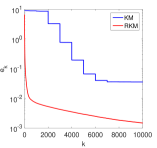
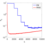
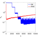
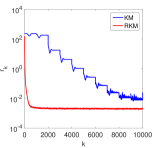
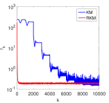
(a) $\delta=0$	(b) $\delta=10^{-3}$	(c) $\delta=10^{-2}$	(d) $\delta=5\times 10^{-2}$

Figure 1: Numerical results ($e_{k}$ and $r_{k}$) for phillips by KM and RKM.

Next we examine the convergence more closely. The (squared) error $e_{k}$ of the Kaczmarz iterate $x_{k}$ undergoes a sudden drop at the end of each cycle, whereas within the cycle, the drop after each Kaczmarz iteration is small. Intuitively, this can be attributed to the fact that the neighboring rows of the matrix $A$ are highly correlated to each other, and thus each single Kaczmarz iteration reduces only very little the (squared) error $e_{k}$, since roughly it repeats the previous projection. The strong correlation between the neighboring rows is the culprit of the slow convergence of the cyclic KM. The randomization ensures that any two rows chosen by two consecutive RKM iterations are less correlated, and thus the iterations are far more effective for reducing the error $e_{k}$, leading to a much faster empirical convergence. These observations hold for both exact and noisy data. For noisy data, the error $e_{k}$ first decreases and then increases for both KM and RKM, and the larger is the noise level $\delta$, and the earlier does the divergence occur. That is, both exhibit a “semiconvergence” phenomenon typical for iterative regularization methods. Thus a suitable stopping criterion is needed. Meanwhile, the residual $r_{k}$ tends to decrease, but for both methods, it oscillates wildly for noisy data and the oscillation magnitude increases with $\delta$. This is due to the nonvanishing variance, cf. the discussions in Section 4. One surprising observation is that a fairly reasonable inverse solution can be obtained by RKM within one cycle of iterations. That is, by ignoring all other cost, RKM can solve the inverse problems reasonably well at a cost less than one full gradient evaluation!

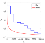
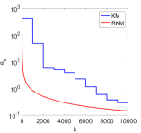
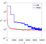
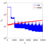
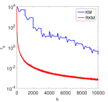
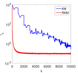
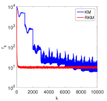
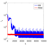
(a) $\delta=0$	(b) $\delta=10^{-3}$	(c) $\delta=10^{-2}$	(d) $\delta=5\times 10^{-2}$

Figure 2: Numerical results ($e_{k}$ and $r_{k}$) for gravity by KM and RKM.

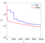
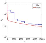
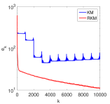
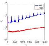
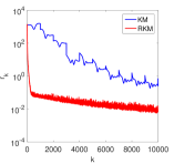
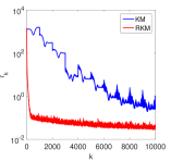
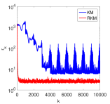
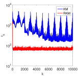
(a) $\delta=0$	(b) $\delta=10^{-3}$	(c) $\delta=10^{-2}$	(d) $\delta=5\times 10^{-2}$

Figure 3: Numerical results ($e_{k}$ and $r_{k}$) for shaw by KM and RKM.

5.2 Preasymptotic convergence

Now we examine the convergence of RKM. Theorems 3.1 and 3.2 predict that during first iterations, the low-frequency error $e_{L}=\mathbb{E}[\|P_{L}e_{k}\|^{2}]$ decreases rapidly, but the high-frequency error $e_{H}=\mathbb{E}[\|P_{H}e_{k}\|^{2}]$ can at best decay mildly. For all examples, the first five singular vectors can capture the majority of the energy of the initial error $x^{*}-x_{0}$. Thus, we choose a truncation level $L=5$, and plot the evolution of low-frequency and high-frequency errors $e_{L}$ and $e_{H}$, and the total error $e=\mathbb{E}[\|e_{k}\|^{2}]$, in Fig. 4.

Numerically, the low-frequency error $e_{L}$ decays much more rapidly during the initial iterations, and since the low-frequency modes are dominant, the total error $e$ also enjoys a very fast initial decay. Intuitively, this behavior may be explained as follows. The rows of the matrix ${A}$ mainly contain low-frequency modes, and thus each RKM iteration tends to mostly decrease the low-frequency error $e_{L}$ of the initial error $x^{*}-x_{0}$. The high-frequency error $e_{H}$ experiences a similar but slower decay during the iteration, and then levels off. These observations fully confirm the preasymptotic analysis in Section 3. For noisy data, the error $e_{k}$ can be highly oscillating, so is the residual $r_{k}$. The larger is the noise level $\delta$, the larger is the oscillation magnitude. However, the degree of ill-posedness of the problem seems not to affect the convergence of RKM, so long as $x^{*}$ is mainly composed of low-frequency modes.

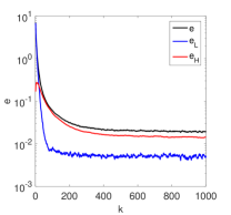
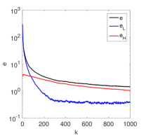
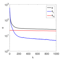
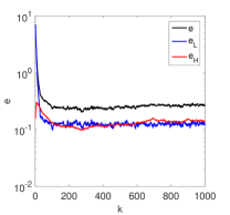
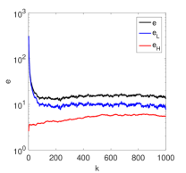
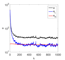
(a) phillips	(b) gravity	(c) shaw

Figure 4: The error decay for the examples with two noise levels: $\delta=10^{-2}$ (top) and $\delta=5\times 10^{-2}$ (bottom), with a truncation level $L=5$.

To shed further insights, we present in Fig. 5 the decay behavior of the low- and high-frequency errors for the example phillips with a random solution whose entries follow the i.i.d. standard normal distribution. Then the source type condition is not verified for the initial error. Now with a truncation level $L=5$, the low-frequency error $e_{L}$ only composes a small fractional of the initial error $e_{0}$. The low-frequency error $e_{L}$ decays rapidly, exhibiting a fast preasymptotic convergence as predicted by Theorem 3.2, but the high-frequency error $e_{H}$ stagnates during the iteration. Thus, in the absence of the smoothness condition on $e_{0}$, RKM is ineffective, thereby supporting Theorems 3.1 and 3.2.

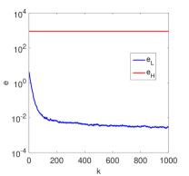
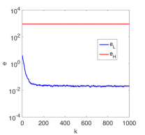
(a) $\delta=10^{-2}$	(b) $\delta=5\times 10^{-2}$

Figure 5: The error decay for phillips with a random solution, with a truncation level $L=5$.

Naturally, one may divide the total error $e$ into more than two frequency bands. The empirical behavior is similar to the case of two frequency bands; see Fig. 6 for an illustration on the example phillips, with four frequency bands. The lowest-frequency error $e_{1}$ decreases fastest, and then the next band $e_{2}$ slightly slower, etc. These observations clearly indicate that even though RKM does not employ the full gradient, the iterates are still mainly concerned with the low-frequency modes during the first iterations, like the Landweber method in the sense that the low-frequency modes are much easier to recover than the high-frequency ones. However, the cost of each RKM iteration is only one $n$th of that for the Landweber method, and thus it is computationally much more efficient.

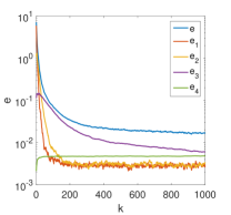
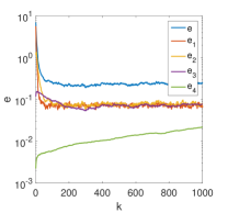
(a) $\delta=10^{-2}$	(b) $\delta=5\times 10^{-2}$

Figure 6: The error decay for phillips. The total error $e$ is divided into four frequency bands: 1-3, 4-6, 7-9, and the remaining, denoted by $e_{i}$, $i=1,\ldots,4$.

5.3 RKM versus RKMVR

The nonvanishing variance of the gradient $g_{i}(x)$ slows down the asymptotic convergence of RKM, and the iterates eventually tend to oscillate wildly in the presence of data noise, cf. the discussion in Section 4. This is expected: the iterate converges to the least-squares solution, which is known to be highly oscillatory for ill-posed inverse problems. Variance reduction is one natural strategy to decrease the variance of the gradient estimate, thereby stabilizing the evolution of the iterates. To illustrate this, we compare the evolution of RKM with RKMVR in Fig. 7. We also include the results by the Landweber method (LM). To compare the iteration complexity only, we count one Landweber iteration as $n$ RKM iterates. The epoch of RKMVR is set to $n$, the total number of data points, as suggested in [19]. Thus $n$ RKMVR iterates include one full gradient evaluation, and it amounts to $2n$ RKM iterates. The full gradient evaluation is indicated by flat segments in the plots.

With the increase of the noise level $\delta$, RKM first decreases the error $e_{k}$, and then increases it, which is especially pronounced at $\delta=5\times 10^{-2}$. This is well reflected by the large oscillations of the iterates. RKMVR tends to stabilize the iteration greatly by removing the large oscillations, and thus its asymptotical behavior resembles closely that of LM. That is, RKMVR inherits the good stability of LM, while retaining the fast initial convergence of RKM. Thus, the stopping criterion, though still needed, is less critical for the RKMVR, which is very beneficial from the practical point of view. In summary, the simple variance reduction scheme in Algorithm 1 can combine the strengths of both worlds.

Last, we numerically examine the regularizing property of RKMVR with the discrepancy principle (4.1). In Fig. 8, we present the number of iterations for several noise levels for RKMVR (one realization) and LM. For both methods, the number of iterations by the discrepancy principle (4.1) appears to decrease with the noise level $\delta$, and RKMVR consistently terminates much earlier than LM, indicating the efficiency of RKMVR. The reconstructions in Fig. 8(d) show that the error increases with the noise level $\delta$, indicating a regularizing property. In contrast, in the absence of the discrepancy principle, the RKMVR iterates eventually diverge as the iteration proceeds, cf. Fig. 7.

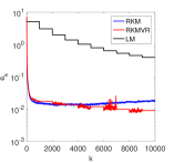
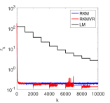
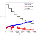
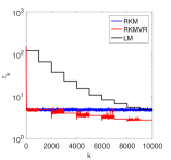
(a) phillips, $\delta=10^{-2}$	(b) phillips, $\delta=5\times 10^{-2}$
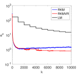
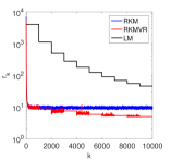
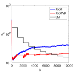
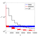
(c) gravity, $\delta=10^{-2}$	(d) gravity, $\delta=5\times 10^{-2}$
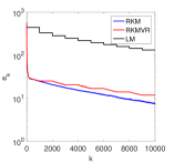
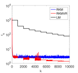
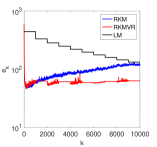
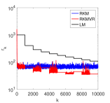
(e) shaw, $\delta=10^{-2}$	(f) shaw, $\delta=5\times 10^{-2}$

Figure 7: Numerical results for the examples by RKM, RKMVR and LM.

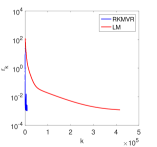
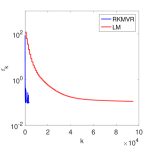
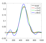
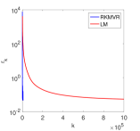
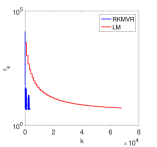
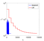
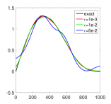
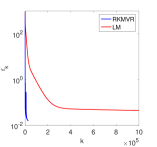
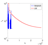
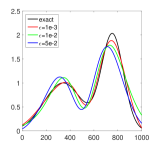
(a) $\delta=10^{-3}$	(b) $\delta=10^{-2}$	(c) $\delta=5\times 10^{-2}$	(d) solutions

Figure 8: The residual $r_{k}$ and the recoveries for phillips (top), gravity (middle), shaw (bottom) by RKMVR and LM with the discrepancy principle (4.1) with $\tau=1.1$.

6 Conclusions

We have presented an analysis of the preasymptotic convergence behavior of the randomized Kaczmarz method. Our analysis indicates that the low-frequency error decays much faster than the high-frequency one during the initial randomized Kaczmarz iterations. Thus, when the low-frequency modes are dominating in the initial error, as typically occurs for inverse problems, the method enjoys very fast initial error reduction. Thus this result sheds insights into the excellent practical performance of the method, which is also numerically confirmed. Next, by interpreting it as a stochastic gradient method, we proposed a randomized Kaczmarz method with variance reduction by hybridizing it with the Landweber method. Our numerical experiments indicate that the strategy is very effective in that it can combine the strengths of both randomized Kaczmarz method and Landweber method.

Our work represents only a first step towards a complete theoretical understanding of the randomized Kaczmarz method and related stochastic gradient methods (e.g., variable step size, and mini-batch version) for efficiently solving inverse problems. There are many important theoretical and practical questions awaiting further research. Theoretically, one outstanding issue is the regularizing property (e.g., consistency, stopping criterion and convergence rates) of the randomized Kaczmarz method from the perspective of classical regularization theory.

References

• [1] A. Agaskar, C. Wang, and Y. M. Lu. Randomized Kaczmarz algorithms: Exact MSE analysis and optimal sampling probabilities. In 2014 IEEE Global Conference on Signal and Information Processing (GlobalSIP), pages 389–393, Atlanta, GA, 2014.
• [2] M. Burger and B. Kaltenbacher. Regularizing Newton-Kaczmarz methods for nonlinear ill-posed problems. SIAM J. Numer. Anal., 44(1):153–182, 2006.
• [3] Y. C. Eldar and D. Needell. Acceleration of randomized Kaczmarz method via the Johnson-Lindenstrauss lemma. Numer. Algorithms, 58(2):163–177, 2011.
• [4] T. Elfving, P. C. Hansen, and T. Nikazad. Semi-convergence properties of Kaczmarz’s method. Inverse Problems, 30(5):055007, 16, 2014.
• [5] H. W. Engl, M. Hanke, and A. Neubauer. Regularization of Inverse Problems. Kluwer, Dordrecht, 1996.
• [6] V. Faber, T. A. Manteuffel, A. B. White, Jr., and G. M. Wing. Asymptotic behavior of singular values and singular functions of certain convolution operators. Comput. Math. Appl. Ser. A, 12(6):733–747, 1986.
• [7] A. Galántai. On the rate of convergence of the alternating projection method in finite dimensional spaces. J. Math. Anal. Appl., 310(1):30–44, 2005.
• [8] G. H. Golub and C. F. Van Loan. Matrix Computations. Johns Hopkins University Press, Baltimore, MD, fourth edition, 2013.
• [9] R. Gordon, R. Bender, and G. Herman. Algebraic reconstruction techniques (ART) for three-dimensional electron microscopy and x-ray photography. J. Theor. Biology, 29(3):471–481, 1970.
• [10] R. M. Gower and P. Richtárik. Randomized iterative methods for linear systems. SIAM J. Matrix Anal. Appl., 36(4):1660–1690, 2015.
• [11] R. M. Gower and P. Richtárik. Stochastic dual ascent for solving linear systems. Preprint, arXiv:1512.06890, 2015.
• [12] M. Haltmeier, A. Leitão, and O. Scherzer. Kaczmarz methods for regularizing nonlinear ill-posed equations. I. Convergence analysis. Inverse Probl. Imaging, 1(2):289–298, 2007.
• [13] P. C. Hansen. Rank-Deficient and Discrete Ill-Posed Problems. SIAM, Philadelphia, PA, 1998. Numerical aspects of linear inversion.
• [14] G. T. Herman, A. Lent, and P. H. Lutz. Relaxation method for image reconstruction. Comm. ACM, 21(2):152–158, 1978.
• [15] G. T. Herman and L. B. Meyer. Algebraic reconstruction techniques can be made computationally efficient. IEEE Trans. Medical Imaging, 12(3):600–609, 1993.
• [16] K. Ito and B. Jin. Inverse Problems: Tikhonov Theory and Algorithms. World Scientific, Hackensack, NJ, 2015.
• [17] Q. Jin. Landweber-kaczmarz method in banach spaces with inexact inner solvers. Inverse Problems, 32(10):104005, 26 pp., 2016.
• [18] Q. Jin and W. Wang. Landweber iteration of Kaczmarz type with general non-smooth convex penalty functionals. Inverse Problems, 29(8):085011, 22, 2013.
• [19] R. Johnson and T. Zhang. Accelerating stochastic gradient descent using predictive variance reduction. NIPS, 2013.
• [20] S. Kaczmarz. Angenäherte Auflösung von Systemen linearer Gleichungen. Bull. Int. Acad. Polon. Sci. Lett. A, 35:335–357, 1937.
• [21] B. Kaltenbacher, A. Neubauer, and O. Scherzer. Iterative Regularization Methods for Nonlinear Ill-posed Problems. Walter de Gruyter GmbH & Co. KG, Berlin, 2008.
• [22] S. Kindermann and A. Leitão. Convergence rates for Kaczmarz-type regularization methods. Inverse Probl. Imaging, 8(1):149–172, 2014.
• [23] R. Kowar and O. Scherzer. Convergence analysis of a Landweber-Kaczmarz method for solving nonlinear ill-posed problems. In Ill-posed and Inverse Problems, pages 253–270. VSP, Zeist, 2002.
• [24] A. Leitão and B. F. Svaiter. On projective Landweber-Kaczmarz methods for solving systems of nonlinear ill-posed equations. Inverse Problems, 32(2):025004, 20, 2016.
• [25] Q. Li, C. Tai, and W. E. Dynamics of stochastic gradient algorithms. preprint, arXiv:1511.06251, 2015.
• [26] A. Ma, D. Needell, and A. Ramdas. Convergence properties of the randomized extended Gauss-Seidel and Kaczmarz methods. SIAM J. Matrix Anal. Appl., 36(4):1590–1604, 2015.
• [27] V. A. Morozov. On the solution of functional equations by the method of regularization. Soviet Math. Dokl., 7:414–417, 1966.
• [28] F. Natterer. The Mathematics of Computerized Tomography. John Wiley & Sons, Ltd., Chichester, 1986.
• [29] D. Needell. Randomized Kaczmarz solver for noisy linear systems. BIT, 50(2):395–403, 2010.
• [30] D. Needell, N. Srebro, and R. Ward. Stochastic gradient descent, weighted sampling, and the randomized Kaczmarz algorithm. Math. Program., Ser. A, 155(1-2):549–573, 2016.
• [31] H. Robbins and S. Monro. A stochastic approximation method. Ann. Math. Stat., 22:400–407, 1951.
• [32] M. Schmidt, N. Le Roux, and F. Bach. Minimizing finite sums with the stochastic average gradient. Math. Progr., 162(1):83–112, 2017.
• [33] F. Schöpfer and D. A. Lorenz. Linear convergence of the randomized sparse Kaczmarz method. Preprint, arXiv:1610.02889, 2016.
• [34] T. Strohmer and R. Vershynin. A randomized Kaczmarz algorithm with exponential convergence. J. Fourier Anal. Appl., 15(2):262–278, 2009.
• [35] C. Wang, A. Agaskar, and Y. M. Lu. Randomized Kaczmarz algorithm for inconsistent linear systems: An exact MSE analysis. In Sampling Theory and Applications (SampTA), 2015 International Conference on, pages 498–502, Washington, DC, 2015.
• [36] A. Zouzias and N. M. Freris. Randomized extended Kaczmarz for solving least squares. SIAM J. Matrix Anal. Appl., 34(2):773–793, 2013.