Universal Linear Mean Relationships in All Polynomials
Abstract
In any cubic polynomial, the average of the slopes at the roots is the negation of the slope at the average of the roots. In any quartic, the average of the slopes at the roots is twice the negation of the slope at the average of the roots. We generalize such situations and present a procedure for determining all such relationships for polynomials of any degree. E.g., in any septic , letting denote the mean value over all zeroes of the derivative , it holds that ; and in any quartic it holds that . Having calculated such relationships in all dimensions up to 49, in all even dimensions there is a single relationship, in all odd dimensions there is a two-dimensional family of relationships. We see connections to Tchebyshev, Bernoulli, & Euler polynomials, and Stirling numbers.
This paper started with (a) the observation that the quadratic formula essentially provides the roots to be where is the mean of the two roots and where is the standard deviation of the two roots considered equally likely, (b) the observation that the slopes at the roots are , and (c) the trivial observation that the average of the slopes at the roots equals the slope at the average of the roots. Curiosity took us next to cubics, to find that the Cardano-Tartaglia cubic formula can be perceived as providing the roots to be where is a primitive cube root of unity, , and where with being the variance of the roots, being the central moment (sometimes referred to as the unscaled skewness), and being the expectation of the roots, considered as being equally likely. Moreover, the coordinates of the cubic’s inflection point are , and the slope at the inflection point is the negation of the mean slope at the roots. Indeed, the inflection point slope will be . Next we saw that the mean slope at the roots of a quartic is the negation of twice the slope at the point and the hunt was on to find all such relationships! It was not just mean slope relationships either– e.g., one can of course note that the mean of a cubic’s function values at the roots of the first derivative equals the ‘mean’ of the function’s (sole) value at the root of the second derivative, viz. . What other relationships lie waiting to be discovered? Have we only seen the tip of an iceberg? Perhaps the reader is starting to suspect that such relationships are really typical.
1 The General Question
We establish some notations. For any degree polynomial let denote the family ( multiset) of roots, and let denote the family of roots of the derivative (sometimes using primemarks for lower orders); we also write (even if some root(s) have multiplicity greater than ). Denote the average value of the function on the derivative roots family as , and similarly use for the average value of the derivative of over the same roots family. Sometimes we will emphasize the degree of by explicitly writing , and we put .
Our initial results mentioned above suggest that we seek to determine
for all & , and that we seek
relationships among various , of the form
. (Other linear
combinations of the that sum over or over
are unnatural because of dimensionality considerations.)
Proof Routes
In cases where the cardinality of the roots family
is or , we can compute by brute
force since the values of the roots will be given by either the quadratic or
cubic formula. Perhaps this method could even be pushed to the case of a
family of roots via the Ferarri quartic formula, but the level of
complexity is greatly increased. In any case, for root families of size
or greater, we need some alternative route.
Again we benefit from establishing notations. We shall use what we refer to
as the quasi-binomial representation of polynomials, expressing coefficients
in terms of averaged symmetric polynomials in the roots. For example, a
general cubic is represented as
where it turns out that
is the average of the roots, is
the average of the products of pairs of roots, and
is the ‘average’ of the
product of triplets of roots. With these, the earlier-mentioned
Cardano-Tartaglia cubic formula can be computed easily via
and
. In general we write
where
denotes that quasi-binomial
parameter with -many bars, , and we write
for the ordered family . Notice that
is just
times the quasi-binomial representation of a generic quadratic. This is
typical: with quasi-binomial representations of polynomials,
, i.e. taking the derivative coincides with truncating the highest order term from the quasi-binomial family ; in other words, for a given quasi-binomial parameter family , we obtain a finite Appell sequence of derived functions. Also, in terms of the
quasi-binomial parameters, the statistically-presented version of the
quadratic formula is simply
.
It remains instructive to establish that the slope of a cubic at its
inflection point is the negated mean of the slopes at the three roots, via the
route of brute force computation. We want to evaluate at the
three roots
(for ): . For this we will use
Now averaging over we encounter convenient terms such
as , and , and three copies of . Hence we obtain
. From the definitions, we
further simplify . Of course . Together
we now have . Whereas the inflection point occurs at , we
also compute , thus establishing our goal.
Looking back, our efforts were aided here by the fact that
, something particular to the case of
cube roots– something that we won’t have available for general cases. What
we will have in the general case is computing means of powers of the roots,
and here is our key to higher degree proofs: we want to be able to express
powers of the roots in terms of the quasi-binomial parameters, i.e. in
terms of the mean elementary symmetric polynomials in the roots.
Exemplifying this in the case of roots, consider:
| (1) |
For any (multi)set of numbers, the elementary symmetric polynomials on are defined as (for ); e.g. if as above with , then is the sum of all products of taking roots at a time, and is the sum of all ‘products’ of taking root at a time. Also define the power sums on per ; . With these definitions, equation (1) above is equivalent to . Such effort to determine the sum of powers (or average of powers) is an established result, the Girard (1629) and Waring (1762) formula [2] which is very closely connected to Newton’s identities (ca. 1687) [10]. Both are based upon the fact that for a (multi)set with it holds that . (Note that .) This relationship can either be solved for the or for the . Solving for an one obtains Newton’s recursive identities . Solving instead for , one obtains the Girard-Waring formula. To state the Girard-Waring formula compactly, Put and consider the -tuples of natural numbers, (), and define with , with being the number of data (or root) values. Note that for is isomorphic to which is the set of integer partitions of ; the only difference (which is insignificant) is that elements of may have trailing zeroes in the partition. E.g., denotes the partition of . The Girard-Waring formula is that , where , where and where is the multinomial coefficient over the family of subindices in . (See Gould [2]). (The are given as sequence A210258 in Sloane’s OEIS [12].) From our perspectives it will become more natural to represent this relationship by replacing and by their normalized forms and , admittedly superficial changes to Girard-Waring. We thus obtain where
| (2) |
We emphasize that for any partition of the power , i.e. , the coefficient of the corresponding term is given by this formula for . By holding fixed all but one of the many parameters in equation (2), one obtains many sequences of coefficients. E.g., the coefficients of for a family of gives sequence (OEIS A080420 [12]) with formula (degree ). E.g., the coefficients of for a family of gives sequence (not in OEIS) with formula (degree ). Tabulated results are in Tables =2 through =7 and in Tables =2 through =7, at the end of the paper. We particularly note that the coefficients in Table =2 are exactly the coefficients of the Tchebyshev polynomials of the first kind. Thus our Tables are generalizations of these Tchebyshev polynomials.
2 Example
An illustrative example is to consider the long-term goal of determining relationships among for . A better example would address for , since with being a quintic we have no hope of algebraically knowing those roots, but the larger example demands much lengthier efforts. So begin with . For , we have the cardinality family , thus quickly we obtain
For , let the family of the roots of the derivative be , and toward determining let us consider . From our mean versions of the Girard-Waring formula (presented as Table =2 at the end of the paper) we have:
, , and .
These give us
| . |
We would be stuck here were it not for the fact that the are roots
of a derivative of , and thus we are blessed with the facts that
and. This is the key issue enabling general degree success.
Thus we substantively extend Girard-Waring by considering
and
where
is the roots family of the derivative
. Simplifying our current degree expression, we
now have
For , let the family of the roots of the derivative be , andtoward determining let us consider . From our mean versions of the Girard-Waring formula (Table =3) we have , , and . These give us
| . |
We would again be stuck here were it not for the fact that the are
roots of a derivative of , and thus we are blessed with the facts that
and
. Simplifying, we now have
Henceforward we shall assume that the leading coefficient is . We have
summarized our
results for other degrees in Tables through at the end of the paper.
We summarize the above procedure. For a given order of derivative,
consider the roots of the derivative, and express the
normalized power sum means in terms of the derivative family’s quasi-binomial
parameters, making use of our normalized variant of the Girard-Waring
formulas. Then to evaluate the mean value of the original degree
function over the derivative roots family, appropriately substitute these
mean power sum expressions in where the argument of the function occurs; this
takes advantage of the fact that averaging is a linear process, to wit, the
mean value of the polynomial function is the sum of the mean values of its
monomial components. Next, taking advantage of the fact that the
quasi-binomial parameters of a family of derivative roots is the same (albeit
truncated) as the quasi-binomial parameters of the degree function, we
are able to simplify the expression of the to be
entirely in terms of the degree function’s quasi-binomial (i.e.
normalized symmetric function) parameters.
With such procedure in hand, we are enabled to determine
general degree results ad libitum. Tabulated results are in Tables
for through , at the end of the paper.
Let us look a bit more closely at the results thus far obtained in the above example. We have:
| , |
| , |
| . |
Observe that all of these have common terms
, so there is more structure here than
what we have put our finger on. After sufficiently inspired inspection we
might realize the following unexpected relationship:
| , | |
| i.e. | |
| ! |
Remarks.
We desire a more systematic way, with less inspiration
required, to obtain such relationships. In effect we are striving to solve
, where the are
“vectors” of linear combinations of the five “basis elements” . Thus the matter of finding all triplet
solutions is a simple
linear algebra issue involving row reduction.
At first glance, trying to solve
for the seems like a
hopeless venture– for this degree case, with basis elements we are
essentially trying to solve equations with only degrees of freedom
in our s. But the fact that all three of the
have common terms
saves us: if we can happen to
satisfy the other three basis elements with s such
that , then
the and constraints will
automatically be satisfied. Besides that, there is further structure within
our results– observe that the coefficients of both
and
are in the proportion . This
again increases our hope of finding at least one
solution triplet.
Observe that: (a) the coefficients within the
are somewhat larger than the coefficients in the
eventual relationship
; and (b) the number of basis elements inside each
is greater than the number of means
in our eventual relationship. These are
typical situations. Indeed, for relationships involving degrees up to ,
we sometimes see coefficients within some in the
tens of thousands, with as many as basis elements, yet the eventual
relationships remain small, with coefficients near , and with to
means involved. The number of basis elements
for different degree polynomials is the number of integer partitions of
the degree (see OEIS A [12]):
| Degree | ||||||||||||
| # Basis Elements |
This all strongly suggests that our proof procedure is unnecessarily
convoluted, and that some more natural and simple proof path is yet to be
found. Streamlined proofs still elude us.
Having noted in the chart above how quickly the number of
basis elements increases with increasing degree, we should be doubtful about
the prospects of finding
solution
tuples for higher degree cases. Our hope rests in there being “special
circumstances” similar to those noted in Remark above.
We shall find that such circumstances do hold.
Before we give a resum\a’e of our complete results, we feel compelled to present the striking degree result: There is a unique solution to , namely
Perhaps equally surprising is that in degree , even though constraints from basis elements must be satisfied, we enjoy a -dimensional family of solution relationships.
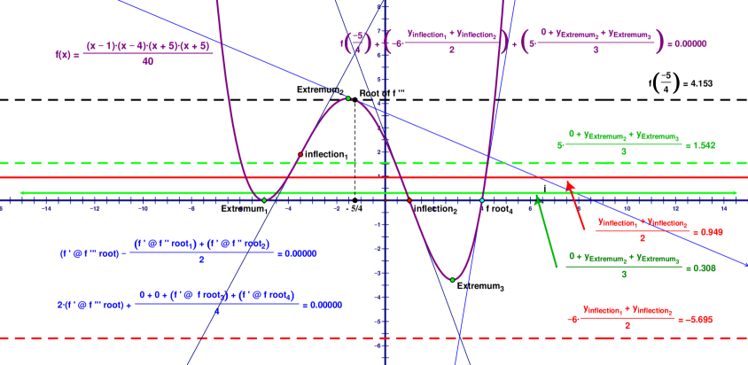
3 Graphical example in degree 4
See Figure 1 at end of paper.
4 Results
The graphical example had us consider which is the average of the slopes at the roots, and this quantity is equal to the negation of twice the slope at the average of the roots. Note that this latter quantity is invariant w.r.t. vertical translations, hence the average of the slopes at the roots does not depend upon the polynomial’s constant term. This is typical:
Proposition 1.
If a horizontal line cuts a polynomial graph at as many points as the degree of the polynomial, the average of the slopes at the points of intersection is invariant w.r.t. modest vertical translations of the line.
Proof.
(Sketch) Given a vertical translation , one can compute changes in the various slopes, ignoring terms that are higher order in . Straightforward algebra shows that the sum of all such slope changes is for degrees through , and we are confident that the same method works in all degrees. ∎
The interpretation of ”modest” in the proposition is that the vertical translation should not cross an extremum. In fact when one accounts for multiplicities and computes, if necessary, complex-valued derivatives for complex-value roots, it is seen that the modesty condition is not a requirement.
Our attempts at an inductive proof of the general case above led to the following confident conjecture (supported by strong numerical evidence). The general proof of proposition 1 would follow as a corollary of the case of the following. Note that the conjecture gives statements in :
Conjecture 1.
In any polynomial of degree with roots set having no repeated roots, it holds that
Note that the above can be reinterpreted as: , the sum of relative rates is where is the roots family of any antiderivative provided that has no repeated roots and that .
We now present some of our results. More completely see Tables through , as well as Tables through , at the end of the paper.
Proposition 2.
The following is an exhaustive list of fundamental linear relationships for degrees up to , among means of a polynomial’s values when evaluated at roots of derivatives.
| A. Degree | N/A |
B. Degree
| (a) |
C. Degree
| (b) |
D. Degree
| (c) | |
| (d) | |
| (any 3 of the above are linearly dependent; any 2 are independent) |
E. Degree
F. Degree
| (any 3 of the above are linearly dependent; any 2 are independent) |
F. Degree
Notes:
The alphabetical labels at the right margins in the preceding & following
propositions indicate “derivative inheritance” relationships across
different degrees.
In all the cases in the above list, the sum of all positive
coefficients equals the sum of all negative coefficients. We have computed such relations up to degree 49, observing that (1) in all even degrees beyond 2 there is a single such fundamental linear relationship, and (2) in all odd degrees beyond 3 there is a 2-dimensional family of fundamental linear relationships. Moreover, the odd degrees enjoy the following clean relationship, which we regard as a main computational result with full confidence.
Conjecture 2.
For all odd degree polynomials of degree , it holds that
There are two ways to augment the above fundamental relationships with more relationships: (a) instead of considering values of the function we can consider values of its derivatives or its (repeated) antiderivatives, which we denote as ; or (b) we can expand the list of root families available by considering the root familes of antiderivatives . When using antiderivatives, it turns out that there is no dependence on the constant of integration; this is a consequence of proposition 1.
Proposition 3.
Expressing polynomials as their quasi-binomial representations, where the constant term of is the constant of integration . In other words, . Restated yet again, if is the quasi-binomial parameter vector of any antiderivative of , then , i.e. is a (strict) subvector of via extension by the constant(s) of integration. Further, if the domain variable of the polynomial carries dimensional units, then the constant is -dimensional.
Dually, if is the quasi-binomial parameter vector of any derivative of , then , i.e. is a (strict) subvector of via truncation.
Example: Consider any polynomial
e.g. with roots family , and consider averaging
the values of the function over some set , . We obtain
. The average values
of the powers are obtained by our mean-value modification of
the Girard-Waring formulas. The case of being the roots
family of a derivative of is straightforward, as noted in the dual statement in the
proposition, with being a
subvector of via truncation.
The case of being the roots family of an antiderivative of
requires greater attention: In the example here, the highest power term
present in is order (& dimensionality if bears units), but the
constant of integration in is of dimensionality ; hence the
constant of integration cannot enter into the computation of
, etc., with similar behavior in the general situation.
Indeed, the values of , etc., only depend upon the entries in
that were already present in
. In the detail of the
present example we have, following our notation for a family of ,
, , and ; thus
| . |
Note, in particular, that the average value does not at all involve the constant of integration that affects the family . This behavior is typical. Let us emphasize: in the computation of mean function values , individual mean powers such as only involve the quasi-binomial parameters of the original and never involve the constant(s) of integration of . Thus we have:
Proposition 4.
The mean quantities and (with ) do not depend on constant(s) of integration.
Proposition 5.
Of course, the above proposition can be read in reverse as
givingand
(with ). These
facts are substantiated in our tables of expressions
by the fact that whenever , the highest order quasi-binomial
parameter is always only order
, never an order in excess of .
For the following five propositions, see also Tables through .
Proposition 6.
The following is a partial list of linear relationships among means of a polynomial’s derivative values when evaluated at roots of derivatives.
| A. | Degree | N/A |
| B. Degree | ||
| (e) |
C. Degree
D. Degree
E. Degree
(any 3 of the above are linearly dependent; any 2 are independent)
Proposition 7.
The following is a partial list of linear relationships among means of a polynomial’s derivative values when evaluated at roots of derivatives.
| A. | Degree | N/A |
| B. | Degree | N/A |
C. Degree
D. Degree
E. Degree
Proposition 8.
The following is a partial list of linear relationships among means of a polynomial’s derivative values when evaluated at roots of derivatives.
| A. | Degree | N/A |
| B. | Degree | N/A |
| C. | Degree | N/A |
D. Degree
E. Degree
Proposition 9.
The following is a partial list of linear relationships among means of a polynomial’s derivative values when evaluated at roots of derivatives.
| A. | Degree | N/A |
| B. | Degree | N/A |
| C. | Degree | N/A |
| D. | Degree | N/A |
E. Degree
Proposition 10.
The following is a partial list of linear relationships
among means of a cubic polynomial’s function, derivatives, and/or
antiderivatives values when evaluated at roots of derivatives and
antiderivatives.
Degree:
The last six of the above deserve particular comment. In the middle three
above, in the first terms (with coefficient ) the cubic function is
being averaged over the root families
, which are
the root families of and. As noted in an
earlier proposition, these results are independent of choice of constants of
integration.
The following essentially restate above results with a different perspective.
See Tables through ,
Note: Regarding the alphabetical labels to the right of some relationships, we have used double-letter hybrid
labels to indicate that the relationship is linearly dependent upon the
denoted pair of preceding relationships, in cases of worthy of attention since the relationship coefficients vector is highly symmetric,
Proposition 11.
In any quartic polynomial the following relations hold:
| (b) | ||
| (f) | ||
| (a’)(a) | ||
| (g) | ||
| . | (e’)(e) |
Proposition 12.
In any quintic polynomial the following relations hold:
| (c) | ||
| (d) | ||
| (cd) | ||
| (b’)(b) | ||
| (h) | ||
| (f’)(f) | ||
| (a”)(a’)(a) | ||
| (i) | ||
| (g’)(g) | ||
| . | (e”)(e’)(e) |
Also note that item states that for any quintic , the average of the function values at the two roots of equals the weighted average of the value of the function at the sole root of and the average of the value of the function at the four roots of . Item states that for any quintic , the average of the function values at the two roots of also equals the weighted average of the value of the function at the sole root of and the average of the value of the function at the three roots of . We leave the remaining interpretations to the reader.
Proposition 13.
In any sextic polynomial the following relations hold:
| (j) | |||
| (c’)(c) | |||
| (d’)(d) | |||
| (b”)(b’)(b) | |||
| (k) | |||
| (h’)(h) | |||
| (f”)(f’)(f) | |||
| (a”’)(a”)(a’)(a) | |||
| (l) | |||
| (i’)(i) | |||
| (g”)(g’)(g) | |||
| (e”’)(e”)(e’)(e) |
Proposition 14.
In any septic polynomial the following relations hold:
| (m) | ||
| (n) | ||
| (mn) |
We find these relationships
distinctively impressive. There are many more identities, not recorded above, that are present when we
open up the limitless world of roots of
, i.e. when we consider the limitless world of mean values
where . See Tables through
.
Ancillary Computational Results
Consider the following observations regarding the coefficients of in . Let be the polynomial in predicting the coefficient of for the family . This polynomial is always of the form where is a monic irreducible (over ) polynomial of degree with integer coefficients, where when is odd and when is even.
Let . Note that (monic condition); also for odd , it holds that & if . The are of the form where is the least common denominator of the terms in , such that is a (generally not monic) polynomial in with integer coefficients, with leading coefficient denoted as .
Curiously, denominators are the OEIS [12] sequence A053657, described in OEIS as “Denominators of integer-valued polynomials on prime numbers (with degree n): 1/a(n) is a generator of the ideal formed by the leading coefficients of integer-valued polynomials on prime numbers with degree less than or equal to n”, or equivalently “Also the least common multiple of the orders of all finite subgroups of [Minkowski]”. Strikingly, the leading coefficients of the polynomials are coefficients of Nørlund’s polynomials, see OEIS A260326 (which had listed only 7 values previous to our work), described there as “Common denominator of coefficients in Nørlund’s polynomial D_2n(x).” [The OEIS citation refers to Nørlund’s 1924 book [8] (which discusses the higher order Bernoulli & Euler polynomials), Table 6 (p. 460), which only lists 7 values, for even indices 0 through 12, but Table 5 (p. 459) includes both even & odd entries as the leading coefficients of the primary components of the numerator polynomials. Our work has produced 198 terms with values eventually exceeding .]
This paper is a spin-off from, and is material to, our recent
Insights Via Representational Naturality: New Surprises Intertwining Statistics, Cardano’s Cubic Formula,
Triangle Geometry, Polynomial Graphs [13].
Here is a summary of our tabulated results.
Tables .D: Function value means in
terms of the polynomial representation parameters . These tables
extend the Girard-Waring formula.
Tables .D: Linear Relationship Coefficients
such that . Some
triplets admit more than one
family.
Tables = through =:
Normalized Girard-Waring coefficients where degree
and where is an integer partition vector of , i.e.
.
Tables .deg= through .deg=:
Normalized Girard-Waring coefficients as above.
(a) [note: ]
(b)
(c)
Supportive Results: Function Value Means
in Terms of Polynomial Representation Parameters .
Table
Table
Table
Tables
–
–
–
–
–
–
–
–
–
–
–
–
–
–
–
–
–
–
–
–
–
–
–
–
–
–
–
–
–
–
–
–
–
–
Tables
Tables
–
–
–
–
–
–
–
–
–
–
–
–
–
–
–
–
–
–
–
–
–
–
–
–
–
–
–
–
–
–
–
–
–
–
Table
Table
–
–
–
–
–
–
–
–
–
–
–
–
–
–
–
–
–
–
–
–
–
–
–
–
–
–
–
–
–
–
–
–
–
Table
Sub-Supportive Normalized Girard-Waring Results
To present our results, let
where is the degree of ;
let let etc. We have the
following results.
N.B.: The coefficients in Table =2 are exactly the coefficients of Tchebyshev polynomials of the first kind. Thus these tables generalize Tchebyshev polynomials.
Table =2
Sum of Positive
Coefficients
Data Family
Table =3
Sum of Positive
Coefficients
Data Family
Table =4
Sum of Positive
Coefficients
Data Family
Table =5
Sum of Positive
Coefficients
Data Family
Table =6
Sum of Positive
Coefficients
Data Family
Collated, instead, along powers, the same information is:
Table deg=2
Sum of Positive
Coefficients
Quadratic
2
2
3
3
4
4
5
5
Table deg=3
Sum of
Coefficients
Cubic
2
3
4
5
Table deg=4
Sum of
Coefficients
Quartic
2
3
4
5
Table deg=5
Sum of
Coefficients
Quintic
2
3
4
5
Table deg=6
Sum of
Coefficients
Sextic
2
3
4
5
9251
Table deg=7
Sum of
Coefficients
Septic
2
3
4
5
-
ACKNOWLEDGMENTS
thanks to all…
References
- 1. E. Barbeau, Polynomials, Springer-Verlag, 1989.
- 2. H. Gould, The Girard-Waring Power Sum Formulas for Symmetric Functions and Fibonacci Sequences, Fibonacci Quaterly, 37(2) (1999), 135-140.
- 3. G. Keady, The Zeros and the Critical Points of a Polynomial: Second Moments and Least Squares Fits of Lines, 2010, accessed 02/17/2014 as https://www.researchgate.net/profile/Grant_Keady/publications/
- 4. G. Keady, Lines of Best Fit for the Zeros and for the Critical Points of a Polynomial, American Mathematical Monthly, 118 (March 2011), 262-264.
- 5. M. Marden, Geometry of Polynomials, Mathematical Surveys No. 3, American Mathematical Society, Providence, RI, 1966.
- 6. M. Marden, Geometry of the Zeros of a Polynomial in a Complex Variable, American Mathematical Society, New York, 1949.
- 7. D. Minda and S. Phelps, Triangles, Ellipses, and Cubic Polynomials, American Mathematical Monthly, 115 (2008), 679-689.
- 8. N. Nørlund, Vorlesungen über Differenzenrechnung, vol. 13 in Die Grundlehren der mathematischen Wissenschaften, Verlag von Julius Springer, Berlin, 1924.
- 9. V. Prasolov, Polynomials, Springer-Verlag 2004.
-
10.
Properties of Polynomial Roots, Wikipedia, accessed 02/13/2014 as
http://en.wikipedia.org/wiki/Properties_of_polynomial_roots - 11. S. Rosset, Normalized Symmetric Functions, Newton’s Inequalities, and a New Set of Stronger Inequalities, American Mathematical Monthly, 96, (1989), 815-819.
- 12. N. Sloane, On-Line Encyclopedia of Integer Sequences, https://oeis.org/
- 13. these authors, Insights Via Representational Naturality: New Surprises Intertwining Statistics, Cardano’s Cubic Formula, Triangle Geometry, Polynomial Graphs, submitted 2017.
-
FIRST AUTHOR
first author
-
2ND AUTHOR
second author
-
3RD AUTHOR
third author