Effect of boson on-site repulsion on the superfluidity
in the boson-fermion-Hubbard model

Abstract

We analyze the finite-temperature phase diagram of the boson-fermion-Hubbard model with Feshbach converting interaction, using the coherent-state path-integral method. We show that depending on the position of the bosonic band, this type of interaction, even if weak, can drive the system into the resonant superfluid phase in the strong bosonic interaction limit. It turns out that this phase can exist for an arbitrary number of fermions (i.e., fermionic concentration between 0 and 2) but with the bosonic particle number very close to an integer value. We point out that the standard time-of-flight method in optical lattice experiments can be an adequate technique to confirm the existence of this resonant phase. Moreover, in the non-resonant regime, the enhancement of the critical temperature of the superfluid phase due to Feshbach interaction is also observed. We account for this interesting phenomena for a hole- or particlelike pairing mechanism depending on the system density and mutual location of the fermionic and bosonic bands.

I Introduction

The boson-fermion-Hubbard model (BFHM) with resonant pairing mechanism has a very long history in the context of high temperature superconductivity (see, e.g. Ranninger and Robaszkiewicz (1985); Robaszkiewicz et al. (1987); Micnas et al. (1990); Friedberg and Lee (1989); Friedberg et al. (1990); Geshkenbein et al. (1997); Neto (2001); Domański and Ranninger (2001); Micnas et al. (2002); Domański et al. (2003); Domański and Ranninger (2004); Micnas et al. (2005); Tsai and Kivelson (2006); Yang et al. (2011); Micnas (2015) and references therein). Recently, the interest in this model has been also extended to the ultracold atomic systems because they are a versatile tool for simulating many-body physics Krutitsky (2016); Bloch et al. (2008, 2012) and BFHM can be studied by using Feshbach resonance experiments in which the BCS-BEC crossover is realized Bloch et al. (2012); Holland et al. (2001); Chen et al. (2005); Ohashi and Griffin (2002).

The impact of strong bosonic interaction on the superfluid (SF) phase in the lattice bosons system has been widely investigated in literature in the terms of Bose-Hubbard model (BHM) (e.g. see Lewenstein et al. (2012) and reference therein). However, the superfluidity in the regime of strong bosonic repulsion in which Feshbach interaction is included is much less understood. So far only hard-core limit Micnas (2007); Cuoco and Ranninger (2006); Ranninger and Tripodi (2003); Micnas et al. (1990); Robaszkiewicz et al. (1987) and some qualitative studies have been performed Zhou and Wu (2006). Therefore in this paper, quantitative investigation of the non-zero temperature BFHM phase diagram with finite bosonic repulsion interaction is carried out, which is relevant for working out realistic experimental conditions. The effective field theory description of the BFHM is constructed by using the coherent state path integral formalism. This analytical method seems to be a good starting point for analysis of BFHM because it provides a reasonable description of the standard Fermi Hubbard model at weak inter-particle interaction (i.e. in the BCS regime) Altland and Simons (2010) and it also gives a correct description of BHM Sengupta and Dupuis (2005). In this paper, we show that besides the standard superfluid phase which is governed by the pure bosonic correlation mechanism present in BHM, there appears also a resonant superfluid (RSF) phase due to Feshbach resonance phenomena. Moreover, we explain that the standard superfluid phase (not RSF) is enhanced by the hole or particle pairing mechanism of fermions. The results allow us to discuss experimental proposal for possible investigation of RSF phase in BFHM.

In the following sections, we first describe the model and the coherent state path integral method applied (Sec. II). Then, in Sec. III, we use this method in analysis of the finite temperature phase diagram of BFHM and its thermodynamic quantities. At the end of Sec. III we also discuss experimental setups that could be used to prove some results of our theory. Finally in Sec. IV we give a summary of our work. Moreover, Appendix A and B contains additional investigation of BFHM model within the operator approach.

II Model and method

II.1 Model

We consider the boson-fermion Hubbard model (BFHM) with converting interaction energy $I$ whose Hamiltonian is given by Micnas (2007, 2015)

$$H=-\sum_{ij\sigma}\left(t_{ij}+\mu\delta_{ij}\right)c_{i\sigma}^{\dagger}c_{j\sigma}-V\sum_{i}c_{i\uparrow}^{\dagger}c_{i\downarrow}^{\dagger}c_{i\downarrow}c_{i\uparrow}$$

$$-\sum_{ij}\left(J_{ij}+\mu^{*}\delta_{ij}\right)b_{i}^{\dagger}b_{j}+\frac{U}{2}\sum_{i}b_{i}^{\dagger}b_{i}^{\dagger}b_{i}b_{i}$$

$$+I\sum_{i}\left[c_{i\uparrow}^{\dagger}c_{i\downarrow}^{\dagger}b_{i}+b_{i}^{\dagger}c_{i\downarrow}c_{i\uparrow}\right],$$ (1)

where $\mu$ is the chemical potential, $\mu^{*}=2\mu-2\Delta_{B}$ and $\sigma$ is a spin$-\frac{1}{2}$ index ($\sigma\in\left\{\uparrow,\downarrow\right\}$). $c_{i\sigma}$ ($c_{i\sigma}^{\dagger}$) is fermionic annihilation (creation) operator at site $i$ with spin $\sigma$ and $b_{i}$ ($b_{i}^{\dagger}$) is bosonic annihilation (creation) operator at site $i$. The hopping energies for fermions and bosons are $t_{ij}$ and $J_{ij}$, respectively. Throughout this work we restrict hopping parameters to the nearest-neighbour sites. Moreover, $U$ denotes the on-site interaction energy of bosons which will be treated exactly during calculations and $V$ is the efermionic on-site interaction strength. The bottom of bosonic band is shifted by $2\Delta_{B}$ parameter which could be tuned in ultracold atoms experiments with the Feshbach resonance Bloch et al. (2012); Holland et al. (2001); Ohashi and Griffin (2002); Ohashi and Griffin (2003a).

Interestingly, if we assume $I=0$ and independent chemical potentials, the BFHM Hamiltonian (Eq. (1)) describes two independent models i.e. the fermionic and bosonic Hubbard models. However, in the presence of finite resonant interaction ($I\neq 0$), there is only one phase transition from the superfluid phase which we will show shortly.

Further, in the case of $U=V=0$ the model described by the Hamiltonian in Eq. (1) has been investigated earlier in the continuum and lattice systems Micnas (2015); Chen et al. (2005); Micnas (2007); Ohashi and Griffin (2003b); Ranninger and Robin (1996, 1997). Moreover, when $U\rightarrow\infty$ the hard-core bosonic limit is obtained for which bosonic operators satisfy the Pauli spin $1/2$ commutations relations Micnas et al. (1990); Micnas (2007); Robaszkiewicz et al. (1987); Micnas (2015); Micnas et al. (2002).

In the coherent state path integral representation, the partition function of BFHM reads

$$Z=\int\mathcal{D}\left[\bar{c},c,\bar{b,}b\right]e^{-\frac{1}{\hbar}S\left[\bar{c,}c,\bar{b,}b\right]},$$ (2)

where the action is given by

$$S\left[\bar{c,}c,\bar{b,}b\right]=S_{0}^{F}\left[\bar{c,}c\right]+S_{0}^{B}\left[\bar{b,}b\right]+S_{0}^{FB}\left[\bar{b,}b,\bar{c,}c\right]+S_{1}^{B}\left[\bar{b,}b\right].$$ (3)

The denotation is related with perturbed and unperturbed parts of the action which we exploit further, i.e. unperturbed parts are

$$S_{0}^{F}\left[\bar{c,}c\right]=\int_{0}^{\hbar\beta}d\tau\left\{\sum_{i\sigma}\bar{c}_{i\sigma}(\tau)\hbar\frac{\partial}{\partial\tau}c_{i\sigma}(\tau)\right.$$

$$+\sum_{ij\sigma}\left(-t_{ij}-\mu\delta_{ij}\right)\bar{c}_{i\sigma}(\tau)c_{j\sigma}(\tau)$$

$$\left.-V\sum_{i}\bar{c}_{i\uparrow}\left(\tau\right)\bar{c}_{i\downarrow}\left(\tau\right)c_{i\downarrow}\left(\tau\right)c_{i\uparrow}\left(\tau\right)\right\},$$ (4)

$$S_{0}^{B}\left[\bar{b,}b\right]=\sum_{i}\int_{0}^{\hbar\beta}d\tau\left\{\bar{b}_{i}(\tau)\hbar\frac{\partial}{\partial\tau}b_{i}(\tau)\right.$$

$$\left.-\mu^{*}\bar{b}_{i}(\tau)b_{i}(\tau)+\frac{U}{2}\bar{b}_{i}(\tau)\bar{b}_{i}(\tau)b_{i}(\tau)b_{i}(\tau)\right\},$$ (5)

$$S_{0}^{FB}\left[\bar{b,}b,\bar{c,}c\right] = I\sum_{i}\int_{0}^{\hbar\beta}d\tau\left[\bar{c}_{i\uparrow}(\tau)\bar{c}_{i\downarrow}(\tau)b_{i}(\tau)+\textrm{c.c.}\right],$$ (6)

and the part of the action which we will be treated approximately is

$$S_{1}^{B}\left[\bar{b,}b\right] = -\sum_{ij}\int_{0}^{\hbar\beta}d\tau J_{ij}\bar{b}_{i}(\tau)b_{j}(\tau)\,.$$ (7)

The fields $c_{i\sigma}\left(\tau\right)$, $\bar{c}_{i\sigma}\left(\tau\right)$ are Grassman variables, the $b_{i}\left(\tau\right)$, $\bar{b}_{i}\left(\tau\right)$ are complex variables, $\hbar$ is reduced Planck constant, $\beta=1/k_{B}T$ where $k_{B}$ and $T$ denote Boltzmann constant and temperature, respectively. Throughout this work we denote the complex conjugation of arbitrary $x$ variable by $\bar{x}$.

II.2 Effective action

We are interested in the influence of the fermionic degrees of freedom on the bosonic part in the BFHM model within the $J\ll U$ limit.

In the first step, the therm describing the interaction between fermionic particles is decoupled by the Hubbard-Stratonovich (HS) transformation in the pairing channel which introduces $\Delta_{i}(\tau),\,\bar{\Delta}_{i}(\tau)$ fields Altland and Simons (2010). Then $S_{0}^{F}\left[\bar{c,}c,\right]\rightarrow\tilde{S}_{0}^{F}\left[\bar{c,}c,\bar{\Delta},\Delta\right]$ where

$$\tilde{S}_{0}^{F}\left[\bar{c,}c,\bar{\Delta},\Delta\right]=\int_{0}^{\hbar\beta}d\tau\left\{\sum_{i\sigma}\bar{c}_{i\sigma}(\tau)\hbar\frac{\partial}{\partial\tau}c_{i\sigma}(\tau)\right.$$

$$-\sum_{i}\bar{c}_{i\uparrow}(\tau)\bar{c}_{i\downarrow}(\tau)\Delta_{i}(\tau)-\sum_{i}\bar{\Delta}_{i}(\tau)c_{i\downarrow}(\tau)c_{i\uparrow}(\tau)$$

$$\left.+\sum_{ij\sigma}\left(-t_{ij}-\mu\delta_{ij}\right)\bar{c}_{i\sigma}(\tau)c_{j\sigma}(\tau)+\frac{1}{V}\sum_{i}\left|\Delta_{i}(\tau)\right|^{2}\right\}\,.$$ (8)

and for which the HS measure $\mathcal{D}\left[\bar{\Delta},\Delta\right]$ contains the determinant $\det\left[V^{-1}\right]$. Then, in the $J\ll U$ limit, we decouple the term in the action from Eq. (7) which is proportional to $J$. It is performed by introducing the HS transformation

$$\sum_{ij}\int_{0}^{\hbar\beta}d\tau J_{ij}\bar{b}_{i}(\tau)b_{j}(\tau)\rightarrow-\sum_{ij}\int_{0}^{\hbar\beta}d\tau J_{ij}^{-1}\bar{\psi}_{i}(\tau)\psi_{j}(\tau)$$

$$+\sum_{i}\int_{0}^{\hbar\beta}d\tau\bar{\psi}_{i}(\tau)b_{i}(\tau)+\sum_{i}\int_{0}^{\hbar\beta}d\tau\bar{b}_{i}(\tau)\psi_{i}(\tau)\,.$$ (9)

Going further, integrating out of bosonic fields $\bar{b}_{i}(\tau)$, $b_{i}(\tau)$ is desirable. Before, we do that, we have to apply some approximation of these fields since in the present form, the action considered above, is non-integrable in $\bar{b}_{i}(\tau)$, $b_{i}(\tau)$ because of the interaction term proportional to $U$. Therefore we rewrite the partition function from Eq. (2) to the following form

$$Z=Z_{0}^{B}\det\left[\mathbf{J}^{-1}\right]\int\mathcal{D}\left[\bar{c},c,\bar{\psi},\psi,\bar{\Delta},\Delta\right]$$

$$\times e^{-\frac{1}{\hbar}\sum_{ij}\int_{0}^{\hbar\beta}d\tau J_{ij}^{-1}\bar{\psi}_{i}(\tau)\psi_{j}(\tau)-\frac{1}{\hbar}\tilde{S}_{0}^{F}\left[\bar{c,}c,\bar{\Delta},\Delta\right]}$$

$$\times\left\langle e^{-\frac{1}{\hbar}\sum_{i}\int_{0}^{\hbar\beta}d\tau\left(\left[-\bar{\psi}_{i}(\tau)+I\bar{c}_{i\uparrow}(\tau)\bar{c}_{i\downarrow}(\tau)\right]b_{i}(\tau)+c.c.\right)}\right\rangle_{0}^{B}$$ (10)

where $\mathbf{J}$ is the hopping matrix $J_{ij}$ which results from the HS transformation in Eq. (9) and the statistical average $\left\langle...\right\rangle_{0}^{B}$ is defined as $\left(Z_{0}^{B}\right)^{-1}\int\mathcal{D}\left[\bar{b},b\right]...e^{-S_{0}^{B}\left[\bar{b,}b\right]/\hbar}$ with

$$Z_{0}^{B}=\int\mathcal{D}\left[\bar{b},b\right]e^{-S_{0}^{B}\left[\bar{b,}b\right]/\hbar}.$$ (11)

Because $\psi_{i}\left(\tau\right)$, $\bar{\psi}_{i}\left(\tau\right)$ fields have quadratic form with linear terms we can make the shift $\psi_{i}(\tau)\rightarrow\psi_{i}(\tau)+Ic_{i\downarrow}(\tau)c_{i\uparrow}(\tau)$ and $\bar{\psi}_{i}(\tau)\rightarrow\bar{\psi}_{i}(\tau)+I\bar{c}_{i\uparrow}(\tau)\bar{c}_{i\downarrow}(\tau)$ and obtain

$$Z=Z_{0}^{B}\det\left[\mathbf{J}^{-1}\right]\int\mathcal{D}\left[\bar{c},c,\bar{\psi},\psi,\bar{\Delta},\Delta\right]$$

$$\times e^{-\frac{1}{\hbar}\sum_{ij}\int_{0}^{\hbar\beta}d\tau J_{ij}^{-1}\left[\bar{\psi}_{i}(\tau)+I\bar{c}_{i\uparrow}(\tau)\bar{c}_{i\downarrow}(\tau)\right]\left[\psi_{j}(\tau)+Ic_{j\downarrow}(\tau)c_{j\uparrow}(\tau)\right]}$$

$$\times e^{-\frac{1}{\hbar}\tilde{S}_{0}^{F}\left[\bar{c,}c,\bar{\Delta},\Delta\right]-\frac{1}{\hbar}W_{1}\left[\bar{\psi,}\psi\right]},$$ (12)

where we define

$$W_{1}\left[\bar{\psi,}\psi\right]=-\hbar\ln\left\langle e^{-\frac{1}{\hbar}\sum_{i}\int_{0}^{\hbar\beta}d\tau\left(-\bar{\psi}_{i}(\tau)b_{i}(\tau)+c.c.\right)}\right\rangle_{0}^{B}.$$ (13)

Within the strong-coupling approach ($J\ll U$) it is convenient to expand $W_{1}\left[\bar{\psi,}\psi\right]$ in terms of $\psi_{i}\left(\tau\right)$, $\bar{\psi}_{i}\left(\tau\right)$ fields, namely

$$W_{1}\left[\bar{\psi,}\psi\right]=\sum_{p=1}^{\infty}\frac{\left(-1\right)^{p}}{\left(p!\right)^{2}}\int_{0}^{\hbar\beta}d\tau_{1}...d\tau_{p}d\tau_{1}^{\prime}...d\tau_{p}^{\prime}$$

$$\times\sum_{i}G_{i}^{p,c}(\tau{}_{1}^{\prime},\,...,\,\tau^{\prime}_{p},\,\tau{}_{1},\,...,\,\tau{}_{p})$$

$$\times\bar{\psi}_{i}(\tau_{1}^{\prime})...\bar{\psi}_{i}(\tau_{p}^{\prime})\psi_{i}(\tau_{1})...\psi_{i}(\tau_{p}),$$ (14)

where $G_{i}^{p,c}(\tau{}_{1}^{\prime},\,...,\,\tau^{\prime}_{p},\,\tau{}_{1},\,...,\,\tau{}_{p})$ are connected local Green functions

$$G_{i}^{p,c}(\tau{}_{1}^{\prime},\,...,\,\tau^{\prime}_{p},\,\tau{}_{1},\,...,\,\tau{}_{p})$$

$$\left.=\frac{\left(-1\right)^{p}\delta^{\left(2p\right)}W_{1}\left[\bar{\psi,}\psi\right]}{\delta\bar{\psi}_{i}(\tau_{1}^{\prime})...\delta\bar{\psi}_{i}(\tau_{p}^{\prime})\delta\psi_{i}(\tau_{1})...\delta\psi_{i}(\tau_{p})}\right|_{\bar{\psi}=\psi=0}.$$ (15)

Then, truncating $W_{1}\left[\bar{\psi,}\psi\right]$ to quartic order and inserting the results to Eq. (12), one gets the following effective action

$$S^{eff}\left[\bar{c},c,\bar{\psi},\psi,\bar{\Delta},\Delta\right]$$

$$=\tilde{S}_{0}^{B}\left[\bar{\psi,}\psi\right]+\sum_{ij}\int_{0}^{\hbar\beta}d\tau\left[\bar{\psi}_{i}(\tau)+I\bar{c}_{i\uparrow}(\tau)\bar{c}_{i\downarrow}(\tau)\right]$$

$$\times J_{ij}^{-1}\left[\psi_{j}(\tau)+Ic_{j\downarrow}(\tau)c_{j\uparrow}(\tau)\right]+\tilde{S}_{0}^{F}\left[\bar{c,}c,\bar{\Delta},\Delta\right]\,$$

$$-\frac{1}{4}\sum_{i}\int_{0}^{\hbar\beta}d\tau d\tau^{\prime}d\tau^{\prime\prime}d\tau^{\prime\prime\prime}G_{i}^{2,c}\left(\tau,\tau^{\prime},\tau^{\prime\prime},\tau^{\prime\prime\prime}\right)$$

$$\times\bar{\psi}_{i}(\tau^{\prime\prime\prime})\bar{\psi}_{i}(\tau^{\prime\prime})\psi_{i}(\tau^{\prime})\psi_{i}(\tau)\,.,$$ (16)

with

$$\tilde{S}_{0}^{B}\left[\bar{\psi,}\psi\right] = \sum_{i}\int_{0}^{\hbar\beta}d\tau d\tau^{\prime}G_{i}^{1,c}\left(\tau,\tau^{\prime}\right)\bar{\psi}_{i}(\tau^{\prime})\psi_{i}(\tau)$$ (17)

It is interesting to point out here that the pair hopping term naturally emerges in the effective action from Eq. (16), i.e. the term $I^{2}\sum_{ij}\int_{0}^{\hbar\beta}d\tau J_{ij}^{-1}\bar{c}_{i\uparrow}(\tau)\bar{c}_{i\downarrow}(\tau)c_{j\downarrow}(\tau)c_{j\uparrow}(\tau)$ and is induced by the resonant interaction $I$.

Further, we perform the second HS transformation in terms of $J_{ij}^{-1}$ , i.e.

$$-\sum_{ij}\int_{0}^{\hbar\beta}d\tau\left[\bar{\psi}_{i}(\tau)+I\bar{c}_{i\uparrow}(\tau)\bar{c}_{i\downarrow}(\tau)\right]$$

$$\times J_{ij}^{-1}\left[\psi_{j}(\tau)+Ic_{j\downarrow}(\tau)c_{j\uparrow}(\tau)\right]$$

$$\rightarrow\sum_{ij}\int_{0}^{\hbar\beta}d\tau J_{ij}\bar{\phi}_{i}(\tau)\phi_{j}(\tau)$$

$$-\left\{\sum_{i}\int_{0}^{\hbar\beta}d\tau\bar{\phi}_{i}(\tau)\left[\psi_{i}(\tau)+Ic_{i\downarrow}(\tau)c_{i\uparrow}(\tau)\right]+c.c.\right\},$$ (18)

where the new HS fields are $\phi_{i}(\tau)$, $\bar{\phi}_{i}(\tau)$. In comparison to the fields from the first HS (Eq. (9)), the $\phi_{i}(\tau)$, $\bar{\phi}_{i}(\tau)$ fields have the same generating functional as the original $b_{i}(\tau)$, $\bar{b}_{i}(\tau)$ fields. Therefore using the $\phi_{i}(\tau)$, $\bar{\phi}_{i}(\tau)$ fields is more suitable in the physical analysis because their correlation functions have the same interpretation as the correlation functions for the original $b_{i}(\tau)$, $\bar{b}_{i}(\tau)$ fields. To clarify this, in Appendix IV.2, we add the proof that both fields have the same generating functional. Moreover, beyond this useful fact about $\phi_{i}(\tau)$, $\bar{\phi}_{i}(\tau)$, it is worth mentioning here that these fields, in the limit of BHM (when $I=0$), yield properly normalized density of states in the BHM superfluid phase Sengupta and Dupuis (2005) (properties of the SF spectrum in the full BFHM need further studies).

After applying second HS (Eq. (18)) to the Eq. (16), corresponding effective action is

$$S^{eff}\left[\bar{c},c,\bar{\phi,}\phi,\bar{\Delta},\Delta\right]$$

$$=-\sum_{ij}\int_{0}^{\hbar\beta}d\tau J_{ij}\bar{\phi}_{i}(\tau)\phi_{j}(\tau)$$

$$+\left\{I\sum_{i}\int_{0}^{\hbar\beta}d\tau\bar{\phi}_{i}(\tau)c_{i\downarrow}(\tau)c_{i\uparrow}(\tau)+c.c.\right\}$$

$$+\tilde{S}_{0}^{F}\left[\bar{c,}c,\bar{\Delta},\Delta\right]+W_{2}\left[\bar{\phi,}\phi\right]\,,$$ (19)

with denotation

$$W_{2}\left[\bar{\phi,}\phi\right]=-\hbar\ln\left\langle e^{-\frac{1}{\hbar}\sum_{i}\int_{0}^{\hbar\beta}d\tau\left(\bar{\phi}_{i}(\tau)\psi_{i}(\tau)+c.c.\right)+\frac{1}{4}\sum_{i}\int_{0}^{\hbar\beta}d\tau d\tau^{\prime}d\tau^{\prime\prime}d\tau^{\prime\prime\prime}G_{i}^{2,c}\left(\tau,\tau^{\prime},\tau^{\prime\prime},\tau^{\prime\prime\prime}\right)\bar{\psi}_{i}(\tau^{\prime\prime\prime})\bar{\psi}_{i}(\tau^{\prime\prime})\psi_{i}(\tau^{\prime})\psi_{i}(\tau)}\right\rangle_{0}^{B,eff},$$ (20)

and where the statistical average $\left\langle...\right\rangle_{0}^{B,eff}$ is defined as $\left(\tilde{Z}_{0}^{B}\right)^{-1}\int\mathcal{D}\left[\bar{\psi},\psi\right]...e^{-\tilde{S}_{0}^{B}/\hbar}$ with $\tilde{Z}_{0}^{B}=\int\mathcal{D}\left[\bar{\psi},\psi\right]e^{-\tilde{S}_{0}^{B}/\hbar}$. And once again truncating $W_{2}\left[\bar{\phi,}\phi\right]$ to the quartic order and retaining only the terms which are not “anomalous” Dupuis (2001); Sengupta and Dupuis (2005); Kennett and Dalidovich (2011); Fitzpatrick and Kennett (2018), we obtained the final form of statistical sum $\tilde{Z}^{eff}$ with effective action $\tilde{S}^{eff}$ (in which the fermionic degrees of freedom were integrated out), i.e.

$$\tilde{Z}^{eff}=\int\mathcal{D}\left[\bar{\phi},\phi,\bar{\Delta},\Delta\right]e^{-\frac{1}{\hbar}\tilde{S}^{eff}\left[\bar{\phi},\phi,\bar{\Delta},\Delta\right]},$$ (21)

$$\tilde{S}^{eff}\left[\bar{\phi},\phi,\bar{\Delta},\Delta\right]=-Tr\ln\left(-G_{F}^{-1}\left(i,\,j,\,\tau\right)\right)+\frac{1}{V}\sum_{i}\left|\Delta_{i}(\tau)\right|^{2}-\sum_{ij}\int_{0}^{\hbar\beta}d\tau J_{ij}\bar{\phi}_{i}(\tau)\phi_{j}(\tau)$$

$$-\sum_{i}\int_{0}^{\hbar\beta}d\tau d\tau^{\prime}\left[G_{i}^{1,c}\left(\tau,\tau^{\prime}\right)\right]^{-1}\bar{\phi}_{i}(\tau^{\prime})\phi_{i}(\tau)+\frac{1}{4}\sum_{i}\int_{0}^{\hbar\beta}d\tau d\tau^{\prime}d\tau^{\prime\prime}d\tau^{\prime\prime\prime}\Gamma_{i}^{2,c}\left(\tau,\tau^{\prime},\tau^{\prime\prime},\tau^{\prime\prime\prime}\right)\bar{\phi}_{i}(\tau^{\prime\prime\prime})\bar{\phi}_{i}(\tau^{\prime\prime})\phi_{i}(\tau^{\prime})\phi_{i}(\tau),$$ (22)

where we introduced the matrix fermionic Green function

$$G_{F}^{-1}\left(i,\,j,\,\tau\right)=$$

$$=\left[\begin{array}[]{cc}\left(-\hbar\frac{\partial}{\partial\tau}+\mu\right)\delta_{ij}+t_{ij}&\Delta_{i}(\tau)-I\phi_{i}(\tau)\\ \bar{\Delta}_{i}(\tau)-I\bar{\phi}_{i}(\tau)&\left(-\hbar\frac{\partial}{\partial\tau}-\mu\right)\delta_{ij}-t_{ij}\end{array}\right],$$ (25)

and effective interaction between bosons

$$\Gamma_{i}^{2,c}\left(\tau,\tau^{\prime},\tau^{\prime\prime},\tau^{\prime\prime\prime}\right)$$

$$\left.=\frac{\delta^{\left(4\right)}W_{2}\left[\bar{\phi,}\phi\right]}{\delta\bar{\phi}_{i}(\tau_{1}^{\prime})\delta\bar{\phi}_{i}(\tau_{2}^{\prime})\delta\phi_{i}(\tau_{1})\delta\phi_{i}(\tau_{2})}\right|_{\bar{\phi}=\phi=0}.$$ (26)

In the following, to analyze the phase diagrams of BFHM, we focus on the saddle point approximation for the effective action from Eq. (22). Moreover, we point out that this effective action could be also used as a starting point for more general considerations which include the fluctuations around saddle point approximation. Formally, it can be performed by expanding $G_{F}^{-1}\left(i,\,j,\,\tau\right)$ in terms of $\Delta_{i}(\tau)-I\phi_{i}(\tau)$ fields.

II.3 Saddle point approximation of the effective action

To investigate the phase diagram which is described by the BFHM effective action from Eq. (22), we apply the mean-field type approximations.

At first, we rewrite Eq. (22) in the Matsubara frequencies ($\omega_{m}$, $\nu_{n}$) and wave vector ($\mathbf{k}$, $\mathbf{q}$, $\mathbf{p}$) representation, which results in $c_{i}(\tau)\rightarrow c_{\mathbf{k}m}$, $\phi_{i}(\tau)\rightarrow\phi_{\mathbf{q}n}$, $\Delta_{i}(\tau)\rightarrow\Delta_{\mathbf{q}n}$. The Matsubara frequencies are defined as $\omega_{m}=\left(2m+1\right)\pi/\beta$ and $\nu_{n}=2n\pi/\beta$ where $m,\,n\in\mathbb{Z}$. Then, applying the Bogoliubov like substitution to the $\phi_{\mathbf{0}0}$ and $\Delta_{\mathbf{0}0}$ components, i.e. $\phi_{\mathbf{0}0}\rightarrow\sqrt{N\hbar\beta}\phi_{0}$ and $\Delta_{\mathbf{0}0}\rightarrow\sqrt{N\hbar\beta}\Delta_{0}$ and omitting the fluctuating bosonic parts $\Delta_{\mathbf{q}n}$ and $\phi_{\mathbf{q}n}$, the mean-field effective action is obtained, i.e.

$$S_{MF}^{eff}=\left\{\epsilon_{\mathbf{0}}-\hbar\left[G^{1,c}\left(i\nu_{n}=0\right)\right]^{-1}\right\}N\hbar\beta\left|\phi_{0}\right|^{2}$$

$$+\frac{g}{2}\left(N\hbar\beta\right)^{2}\left|\phi_{0}\right|^{4}+\frac{N\hbar\beta}{V}\left|\Delta_{0}\right|^{2}$$

$$-\mathrm{Tr}\ln\left(-N\beta G_{F}^{-1}\left(i\omega_{m},\,\mathbf{k}\right)\right)\,,$$ (27)

where

$$G_{F}^{-1}\left(\mathbf{k},\,i\nu_{m}\right)=\left[\begin{array}[]{cc}i\hbar\omega_{m}-\xi_{\mathbf{k}}&\Delta_{0}-I\phi_{0}\\ \bar{\Delta}_{0}-I\bar{\phi}_{0}&i\hbar\omega_{m}+\xi_{\mathbf{k}}\end{array}\right]\,,$$ (28)

with $\epsilon_{\mathbf{q}}=-2J\sum_{\alpha}\cos q_{\alpha}$, $\xi_{\mathbf{k}}=t_{\mathbf{k}}-\mu$, $t_{\mathbf{k}}=-2t\sum_{\alpha}\cos k_{\alpha}$ (symbol $\alpha\in\left\{x,\,y,\,z\right\}$ denotes Cartesian coordinates). Moreover, in further calculations we also define coordinate number $z=6$ which is related to the $\epsilon_{\mathbf{q}}$ by expression $\epsilon_{\mathbf{0}}=-Jz$. Here, we restrict our consideration to the simple cubic lattices. The explicit form of $G^{1,c}\left(i\nu_{n}\right)$ is given in Appendix IV.1. Moreover, in Eq. (27) we use static approximation to the $\Gamma_{i}^{2,c}$ function and denote this limit by $2g$ (here we do not use the explicit form of $g$ but it could be found in Ref. Sengupta and Dupuis (2005)).

To describe the ordered phase in terms of $\phi_{0}$ and $\Delta_{0}$ we calculate the saddle point of the above effective action

$$\frac{\partial}{\partial\bar{b}_{0}}S_{MF}^{eff}=0\,,$$ (29)

$$\frac{\partial}{\partial\bar{\Delta}_{0}}S_{MF}^{eff}=0\,.$$ (30)

This results in the following coupled equations

$$\left\{\begin{array}[]{l}\left\{\epsilon_{\mathbf{0}}-\hbar\left[G^{1,c}\left(i\nu_{n}=0\right)\right]^{-1}\right\}\phi_{0}+gN\hbar\beta\left|\phi_{0}\right|^{2}\phi_{0}=-\frac{I}{N\hbar\beta}\sum_{m\mathbf{k}}G_{F}^{12}\left(\mathbf{k},\,i\hbar\omega_{m}\right)=-\frac{I}{N}\sum_{\mathbf{k}}\frac{\left(Vx_{0}-I\phi_{0}\right)}{2E_{\mathbf{k}}}\tanh\left(\frac{\beta}{2}E_{\mathbf{k}}\right),\\ x_{0}=\frac{1}{N\hbar\beta}\sum_{m\mathbf{k}}G_{F}^{12}\left(\mathbf{k},\,i\hbar\omega_{m}\right)=\frac{1}{N}\sum_{\mathbf{k}}\frac{\left(Vx_{0}-I\phi_{0}\right)}{2E_{\mathbf{k}}}\tanh\left(\frac{\beta}{2}E_{\mathbf{k}}\right),\end{array}\right.$$ (31)

where $Vx_{0}=\Delta_{0}$ and

$$E_{\mathbf{k}}=\sqrt{\xi_{\mathbf{k}}^{2}+\left|I\phi_{0}-Vx_{0}\right|^{2}}\,.$$ (32)

From Eqs. (31) one immediately sees that $x_{0}$ and $\phi_{0}$ are non-linearly coupled to each other, i.e.

$$\left\{\epsilon_{\mathbf{0}}-\hbar\left[G^{1,c}\left(i\nu_{n}=0\right)\right]^{-1}\right\}\phi_{0}+gN\hbar\beta\left|\phi_{0}\right|^{2}\phi_{0}=-Ix_{0}.$$ (33)

which suggests that there is only one phase transition from the superfluid phase to normal phase.

Moreover, it is interesting to point out here, that above equation correctly recovers the limiting cases of non-interacting ($U=0$) and hard core ($U\rightarrow\infty$) bosons (in which fermionic interaction can be finite i.e. $V\neq 0$). For $U=0$ the term with $g$ disappears and one has $\hbar\left[G^{1,c}\left(i\nu_{n}=0\right)\right]^{-1}=\mu^{*}$, therefore

$$\phi_{0}=\frac{-I}{\epsilon_{\mathbf{0}}-\left(2\mu-2\Delta_{B}\right)}x_{0}\,,$$ (34)

which corresponds to the well-known result without a lattice Ohashi and Griffin (2003b). For $U\rightarrow\infty$, two Fock states are taken in Eq. (42), i.e. $n_{0}=0,\,1$, which gives $\hbar\left[G^{1,c}\left(i\nu_{n}=0\right)\right]^{-1}=\mu^{*}/\left(1-2n_{B,0}\right)$ with $n_{B,0}=e^{\beta\mu^{*}}/(1+e^{\beta\mu^{*}})$. Therefore, for the hard-core bosons case one gets

$$\phi_{0}=\left(Ix_{0}+\epsilon_{\mathbf{0}}\phi_{0}\right)\frac{1-2n_{B,0}}{2\mu-2\Delta_{B}}\,,$$ (35)

where we neglect the contribution from $g$ term by assuming a limit of small order parameter $\phi_{0}$. This result (Eq. (35)) recovers the previous one from Ref. Robaszkiewicz et al. (1987).

We have also confirmed that Eqs. (31), in the limit of small amplitude of $\phi_{0}$ (in which the term proportional to $g$ could be neglected), can be recovered from the mean-field and linear response considerations, see Appendix IV.3. Therefore, these both approaches lead to the same equation for critical line considered in the rest of the paper.

At the end of this subsection, it is worth pointing out that the results, obtained in Secs. II.2 and II.3, are quite general and can be used for further analytical and numerical considerations in which $I$, $U$ and $V$ interactions are finite quantities. These results are interested on its own right and can be applied to study of e.g. superfluidity or critical phenomena. In our further analysis, we focus on the specific physical regime of derived theory in which BHM is set as our reference point.

II.4 Phase diagram

In this work, we are interested in the phase diagram of strongly correlated bosonic regime ($J\ll U$). Therefore, at the phase boundary where $x_{0}\rightarrow 0,\>\phi_{0}\rightarrow 0$ in Eqs. (31), critical line is obtained from

$$\epsilon_{\mathbf{0}}-\hbar[G^{1,c}\left(i\nu_{n}=0\right)]^{-1}=\frac{I^{2}\Pi(T_{c})}{1-V\Pi(T_{c})},$$ (36)

where

$$\Pi(T_{c})=\frac{1}{N}\sum_{\mathbf{k}}\frac{1}{2\xi_{\mathbf{k}}}\tanh\left(\frac{\xi_{\mathbf{k}}}{2k_{B}T_{c}}\right).$$ (37)

It is interesting to notice here that in the case of $I=0$, the Eq. (36) and the equation in the second line of (31), get the forms which are known in the phase diagram analysis of BHM and BCS systems, respectively.

However, in our furhter analysis, we limit considerations to the case of $V=0$ for simplicity. Therefore we focus on the paring mechanism of fermions which comes from the converting interactions $I$. Then, by direct substitution of $V=0$ to the Eq. (36), the phase boundary in BFHM is obtained from the equation

$$\epsilon_{\mathbf{0}}-\hbar[G^{1,c}\left(i\nu_{n}=0\right)]^{-1}=I^{2}\Pi(T_{c}).$$ (38)

In further discussion we set $\hbar=1$ and $k_{B}=1$ for simplicity.

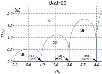
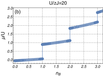
Figure 1: (a) Mean-field phase diagram of BHM (temperature $T/Jz$ versus average particle number per site $n_{B}$). (b) Chemical potential $\mu/U$ versus $n_{B}$ calculated along the critical line from Fig. (a). For clarity, the circles are added on the numerical data points in Fig. (b).

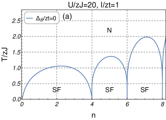
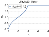
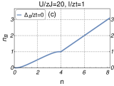
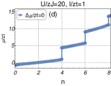
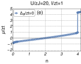
Figure 2: (a) Finite temperature mean-field phase diagram of BFHM versus total particle number $n=2n_{B}+n_{F}$ for zero detuning of parameter $\Delta_{B}$. Figures (b), (c), (d) are plots of $n_{F}$, $n_{B}$, $\mu/zt$ versus $n$, respectively (the data obtained are evaluated along the critical line from Fig. (a)). Figure (e) is an enlargement of the vicinity of zero chemical potential from plot (d). Plots are made assuming that $U/zJ=20$, $I/zt=1$, $J=t/2$. For clarity, the circles are added on the numerical data points in Figs. (d) and (e).

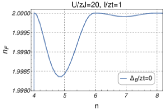
Figure 3: Dependence of fermionic density $n_{F}$ on the total particle density $n$. This figure is an enlargement of the $n\in(4,8)$ region from Fig. 2 b.

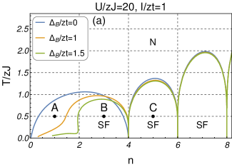
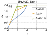
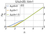
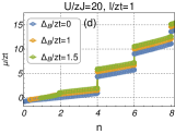
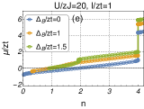
Figure 4: (a) Finite temperature mean-field phase diagram of BFHM versus total particle number $n=2n_{B}+n_{F}$ for different strengths of detuning $\Delta_{B}$ (see legend). Figures (b), (c), (d) are plots of $n_{F}$, $n_{B}$, $\mu/zt$ versus $n$, respectively (the data obtained are evaluated along the critical line from Fig. (a)). Figure (e) is an enlargement of the vicinity of zero chemical potential from plot (d). Plots are made assuming that $U/zJ=20$, $I/zt=1$, $J=t/2$. For comparison, we plot $\Delta_{B}/zt=0$ from Fig. 2. For clarity, the circles are added on the numerical data points in Figs. (d) and (e). Meaning of A, B and C points is given in Sec. III.6.

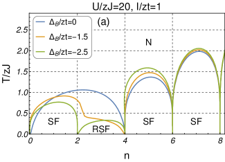
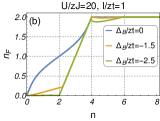
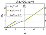
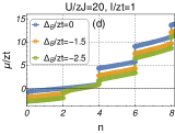
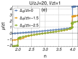
Figure 5: (a) Finite temperature mean-field phase diagram of BFHM versus total particle number $n=2n_{B}+n_{F}$ for different strengths of detuning parameter $\Delta_{B}$ (see legend). Figures (b), (c), (d) are plots of $n_{F}$, $n_{B}$, $\mu/zt$ versus $n$, respectively (the data obtained are evaluated along the critical line from Fig. (a)). Figure (e) is an enlargement of the vicinity of zero chemical potential from plot (d). Plots are made assuming that $U/zJ=20$, $I/zt=1$, $J=t/2$. For comparison, we plot $\Delta_{B}/zt=0$ from Fig. 2. For clarity, the circles are added on the numerical data points in Figs. (d) and (e).

II.5 Average particle number

During the analysis of the boson-fermion mixture phase diagram in the following sections, the additional considerations of the average particle number per site $n$ are made; $n$ is calculated within the unperturbed part of the action from Eq. (3) at the phase boundary (it is consistent with the mean-field calculation of average particle number per site at phase boundary within the operator approach method, see Appendix IV.3). This means that the $0$-th order partition function has the form $Z_{0}=Z_{0}^{F}Z_{0}^{B}$ where $Z_{0}^{F}=\int\mathcal{D}\left[\bar{c},c\right]e^{-S_{0}^{F}\left[\bar{c,}c\right]/\hbar}$ and $Z_{0}^{B}$ is defined in Eq. (11). Therefore $n$ is calculated by using $n=-\partial\ln Z_{0}/\partial\mu$ and we get

$$n=n_{F}+2n_{B}\;,$$ (39)

where $n_{F}$ is the average particle number of fermions for both spin components

$$n_{F}=2\sum_{\mathbf{k}}\frac{1}{e^{\beta\left(t_{\mathbf{k}}-\mu\right)}+1}\;,$$ (40)

and $n_{B}$ is an average particle number of bosons

$$n_{B}=\frac{\sum_{n_{0}=0}^{\infty}n_{0}e^{-\beta E_{n_{0}}}}{\sum_{n_{0}=0}^{\infty}e^{-\beta E_{n_{0}}}}\;,$$ (41)

where on-site bosonic energy $E_{n_{0}}$ is defined in Eq. (43). There is also a possibility to obtain Eqs. (39-41) directly by taking into account Gaussian fluctuations over a saddle point action $S_{MF}^{eff}$ from Eq. (27) at the phase boundary.

It is also worth adding here that improved approach which includes the effect of resonant interaction $I$, bosonic hopping $J$ and fermionic interaction $V$, in the normal phase, can be achieved by using the self-consistent T-matrix theory Micnas (2015, 2007).

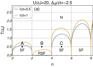
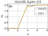
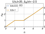
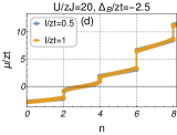
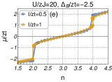
Figure 6: (a) Finite temperature phase diagram of BFHM versus total particle number $n=2n_{B}+n_{F}$ for different strengths of converting interaction $I/zt$ (see legend). Figures (b), (c), (d) are plots of $n_{F}$, $n_{B}$, $\mu/zt$ versus $n$, respectively (the data obtained are evaluated along the critical line from Fig. (a)). Figure (e) is an enlargement of the vicinity of zero chemical potential from plot (d). Plots are made assuming that $U/zJ=20$, $\Delta_{B}/zt=-2.5$, $J=t/2$. For clarity, the circles are added on the numerical data points in Figs. (d) and (e). Meaning of A, B and C points is given in Sec. III.6.

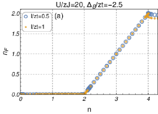
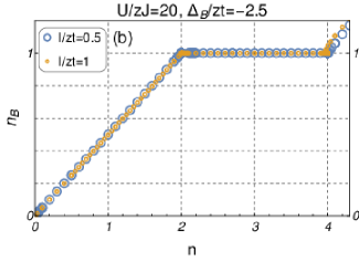
Figure 7: Plots a and b are enlargements of the relevant parts of Figs. 6 b and c, respectively.

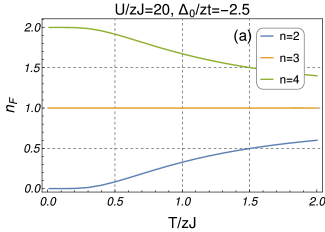
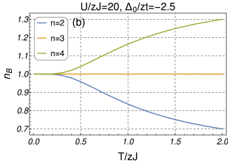
Figure 8: Fermionic $n_{F}$ (a) and bosonic $n_{B}$ (b) average particle density per site with fixed total number of particles $n=n_{F}+2n_{B}$ (see Eqs. (39)-(41)). The other parameters are $U/zJ=20$, $J=t/2$.

III Results and discussion

III.1 Phase diagram of the BHM

In order to clarify further discussion, we shortly review the finite temperature phase diagram of the standard BHM in terms of reduced critical temperature $T_{c}/zJ$ versus average concentration of bosons per site $n_{B}$.

Using previously defined bosonic annihilation and creation operators $b_{i}$ and $b_{i}^{\dagger}$, BHM Hamitonian has the form $H_{BHM}=-\sum_{ij}\left(J_{ij}+\mu\delta_{ij}\right)b_{i}^{\dagger}b_{j}+U\sum_{i}b_{i}^{\dagger}b_{i}^{\dagger}b_{i}b_{i}$. The phase diagram comprising SF, bosonic Mott insulator (BMI) and normal (N) phases is well-known Sheshadri et al. (1993); Trotzky et al. (2010); Sajna et al. (2015) and in the mean-field approximation the critical line is given by $\epsilon_{\mathbf{0}}-\left[G^{1,c}\left(i\nu_{n}=0\right)\right]^{-1}=0$. In Fig. 1, we plot critical temperature $T_{c}/zJ$ dependence on the average density of bosons per site $n_{B}$ for the critical boundary in BHM. BMI for different integer values of $n_{B}$ are located only between lobes at zero temperatures which are indicated in Fig. 1 by black arrows (at finite temperatures there is no true insulating state Gerbier (2007)). Here and in the following subsection we choose $U/Jz=20$ to analyze strong interaction limit of bosonic particles.

III.2 Density phase diagram of BFHM model

We are interested in the density phase diagram of BFHM in the limit $J\ll U$ and $V=0$ (as was mentioned in Sec. II.4). The critical boundary line at finite temperatures is obtained from Eq. (38). In the following subsections III.3, III.5, III.4, the phase diagram of BFHM is analyzed in three different regimes of parameter $\Delta_{B}$ which controls mutual position of fermionic and bosonic band, namely: (a) $\Delta_{B}/zt=0$, (b) $\Delta_{B}/zt>0$, (c) $\Delta_{B}/zt<0$. In particular, the value of parameter $\Delta_{B}$ is directly related to the position of the bottom of bosonic band with respect to that of fermionic one. It is clear from considering BFHM Hamiltonian from Eq. (1) and from relation $J=t/2$ which corresponds to assumption that one molecule is made of two fermionic particles. The bottom of the boson band is located at the center of the fermion band at $\Delta_{B}/zt=0.25$ and it starts to appear below the fermionic band for $\Delta_{B}/zt<-0.75$ and above for $\Delta_{B}/zt>1.25$.

III.3 Zero detuning ($\Delta_{B}=0$)

In Fig. 2, we show the finite temperature phase diagram for BFHM with zero detuning $\Delta_{B}/zt=0$, finite bosonic interaction strength $U/zJ=20$ and converting interaction $I/zt=1$. These results explicitly show that if $\Delta_{B}/zt=0$ parameter is close to $\Delta_{B}/zt=0.25$ value (i.e. bottom of bosonic band is close to the middle of fermionic one), the critical line assumes a regular lobe structure similarly like in the phase diagram of standard BHM (see Fig. 1). However, in BFHM case the lowest lobe is relatively wider than the others (i.e. $n\in\left(0,4\right)$ instead of width $2$ in $n$ units in comparison to pure BHM case, see. Fig. 1). This widening is related to the gradual filling up of the fermionic band with increasing value of total particles $n$ (see, Fig. 2 b). Indeed, chemical potential gradually crosses the fermionic band which is clearly visible in Fig. 2 d and e, i.e. $\mu/zt$ appear at the bottom of fermionic band ($\mu=-zt$) at $n=0$ and ending at the top of fermionic band ($\mu=zt$) for $n=4$.

It is interesting to notice here that in comparison to the BHM case (Fig. 1), there is an enhancement of the superfluid critical temperature when $I\neq 0$. Starting from second lobe, this enhancement can be simple accounted for the pairing mechanism of fermionic holes. This is confirmed by the slight deviations of fermionic density from a band insulator regime ($n_{F}=2$) for $n>4$ (see Fig. 2 b and its corresponding enlargement in Fig. 3).

The above picture is dramatically changed when detuning starts to deviate from zero value. It will be discussed below.

III.4 Positive detuning ($\Delta_{B}>0$)

With increasing value of $\Delta_{B}/zt$ parameter, the bottom of bosonic band is above the fermionic one for $\Delta_{B}/zt>1.25$. This should result in increasing fermionic density at the expense of bosonic one at low $n$ which indeed is clearly visible in Fig. 4 a-c. In particular, with increasing $\Delta_{B}/zt$, the lower part of the first lobe gradually diminishes and the first lobe-like structure appears for $n\in\left(2,4\right)$ (see, Fig. 4 with $\Delta_{B}/zt=1.5$). Such a situation is also confirmed by analysis of the chemical potential $\mu/zt$ (see, Fig. 4 d and e) which shows that its value starts to appear only in region of fermionic band for $n\in\left(0,\,2\right)$ and for higher values of $\Delta_{B}/zt$ for which the bosonic density is very low (it should be compared to the situation with $\Delta_{B}/zt=0$ in which $\mu\in\left\langle-zt,\,zt\right\rangle$ for $n\in\left(0,\,4\right)$, Fig. 4 d and e).

III.5 Negative detuning ($\Delta_{B}<0$)

The situation is even more interesting for negative detuning for which the bottom of bosonic band is below the fermionic one for $\Delta_{B}/zt<-0.75$. Intuitively, when the number of particles $n$ is increased, at first the bosonic band should start to fill up. This intuition fully agrees with our simulation presented in Fig. 5 for $n_{B}$ and $n_{F}$ versus $n$ and is clearly observed in the regime of relatively high negative values of $\Delta_{B}/zt=-2.5$. However, in comparison to the reference case at $\Delta_{B}/zt=0$ the situation here is more complex, the critical line at $\Delta_{B}/zt=-2.5$ for $n\in\left\langle 0,\,4\right\rangle$ range decays into two lobes (see, Fig. 5 a). The first lobe at $n\in\left\langle 0,\,2\right\rangle$ contains the SF phase with gradually increasing average number of bosonic particles $n_{B}$ (Fig. 5 c) and the second lobe at $n\in\left\langle 2,\,4\right\rangle$ is characterized by the almost integer bosonic density $n_{B}$ (here close to one) i.e. it has the BMI character for bosonic particles (the bosonic density deviates from the integer number with order less than $10^{-6}$) (Fig. 5 c). Moreover, the fermionic part for $n\in\left\langle 2,\,4\right\rangle$ gradually changes its density from $n_{F}=0$ to $n_{F}=2$ with increasing value of $n$. We also clearly see, that the phase is characterized by location of chemical potential inside the fermionic band, pointing out that the system is at the Feshbach resonance (see, Fig. 5 d and e). Further, we argue that this superfluid phase with number of bosons close to integer value arises purely from the resonant mechanism and for simplicity we denote it as resonant superfluid (RSF) phase.

To show the resonant character of RSF we check the sensitivity of this phase by tuning the amplitude of converting interaction in $S_{0}^{FB}$ from Eq. (3). Namely, in Fig. 6 we plot the phase diagram for different values of $I/zt$. This phase diagram shows that the RSF phase is highly suppressed at finite temperatures and it almost disappear for $I/zt=0.5$. Therefore one can conclude that RSF phase originates from the Feshbach-like correlations.

Moreover, it is worth adding here, that fermionic $n_{F}$ and bosonic $n_{B}$ densities are almost intact with respect to the change of $I/zt$ in RSF phase (see Fig. 6 b, c and 7). However, as expected we observe, that there is a slight change of these densities not visible in the presented density plots (the order of this change is less than $10^{-6}$).

We also checked the vicinity of the RSF region by analyzing normal phase above the critical temperature in terms of $n_{F}$ and $n_{B}$ densities at a constant $n$ (see, Fig. 8). These densities correspond to the $I/zt=0$ regime at this level of approximation (see Sec. II.5 and Eqs. (39-41). From Fig. 8, we observe that in the $T\rightarrow 0$ limit, $n_{B}$ is pinned to the integer value equal to one while $n_{F}$ gradually increases for the corresponding total particle density $n=2,\,3,\,4$. This observation is consistent with the conclusion about RSF phase drawn in the previous paragraph.

It is also worth adding here, that the above picture of BFHM phase diagram is also consistent with the work Micnas et al. (2003) which considered the hard-core limit of bosonic particles without bosonic hopping ($J=0$). It should not be surprising because our theory properly recover this limit at the mean-field level (see, Eq. 35). However, RSF phase with the number of bosons close to one is a novel behavior which appears beyond the hard-core limit.

Moreover, when the system is beyond the Feshbach resonance for $\Delta_{B}/zt=-2.5$ (i.e. chemical potential is below or above fermionic band) there is another interesting feature observed in Fig. 6. Namely, the SF phase is favored for $n\in\left(0,\,2\right)$ and $n>4$, but it is important to point out here that the mechanism behind it is quite different. In the $n\in\left(0,\,2\right)$ range SF is enhanced through paring of fermionic particles (BCS like character), but in the $n>4$ range paring mechanism is through fermionic holes. It is indicated by the corresponding low magnitude enhancement (for $n\in\left(0,\,2\right)$) or reduction (for $n>4$) of the fermionic density part in numerical data.

At the end of this section, we would like to also add that for higher values of negative detuning $\Delta_{B}/zt$, the general behavior of phase boundary is similar to that discussed above. Namely, higher negative values of $\Delta_{B}/zt$ shift of chemical potential also to higher negative values causing that Feshbach resonance region around $\mu/zt\in\left\langle-1,\,1\right\rangle$ appears for higher densities. Then, depending on the $\Delta_{B}/zt$ value, a situation like that in the former cases appears, i.e. (1) the widening of one of the lobes like for $\Delta_{B}/zt=0$ (see, Fig. 4) or (2) the emergence of RSF mixture like for $\Delta_{B}/zt=-2.5$ (see, Fig. 5). In particular, up to $\Delta_{B}/zt=-10$ with the same BFHM Hamiltonian parameters as before, we numerically check, that the first situation (1) appears for $\Delta_{B}/zt=-5$ and $\Delta_{B}/zt=-10$ and the second one (2) appears for $\Delta_{B}/zt=-7.5$ (here RSF phase emerge for $n\in\left(4,\,6\right)$).

It would be also interesting in further investigations beyond mean-field approximation, to include the effects of pairing fluctuations into theory which should imply lowering of superfluid critical temperature. Then the temperature obtained in this work will correspond to the appearance of the pseudogap regime for fermionic particles Micnas (2015, 2007); Micnas et al. (2002).

III.6 RSF phase in the time of flight type experiment

Time of flight (TOF) type spectroscopy is one of the most powerful methods of measurements in the state of art of current experimental setups in ultracold atoms. Within the optical lattice systems, it has been widely used for e.g. bosons Kennedy et al. (2015); Gerbier et al. (2008); Spielman et al. (2007); Gerbier et al. (2005); Greiner et al. (2002), fermions Rom et al. (2006); Chin et al. (2006) or boson-fermion mixtures Best et al. (2009); Günter et al. (2006). In particular, it is relatively simple to probe coherence via momentum distribution encoded in freely expanding cloud. As an example, it has been previously used to detect SF-BMI quantum phase transition in the bosonic Rb atoms Greiner et al. (2002) or resonant superfluidity in the fermionic Li atoms Chin et al. (2006). In a realistic experiment, the enhancement of coherence is observed as the appearance of peaks in the time of flight pattern Kennedy et al. (2015); Chin et al. (2006); Gerbier et al. (2005); Greiner et al. (2002).

We suggest that the footprint of the RSF phase can be tested by preparing ultracold fermionic gas at the Feshbach resonance with negative detuning of $\Delta_{B}$ parameter. The detuning should be about two and half times greater than the width of the fermionic band. Then repeating the experiment with increasing number of fermions which simulate BFHM (which is close to the ground state), one should observe a lowering of coherence at $n\in\left\langle 2,\,4\right\rangle$ densities. It can be deduced from the phase diagram in Fig. 6 where in the range $n\in\left(0,\,2\right)$ and $n>4$, SF phase has a higher critical temperature than in the $n\in(2,\,4)$ region.

For instance, let’s assume that the atomic gas is prepared at similar temperatures for different particle numbers which are represented by points A, B and C in Figs. 4 a and 6 a. Furthermore, let’s assume that in each of these phases represented by points A, B and C, TOF experiment is performed. Then, it can be concluded that for the situation with positive detuning as in Fig. 4 a, the coherence of bosonic particles should be an increasing function of $n$ at corresponding points A, B and C, because of the deeper penetration of the system into SF phase for A, B and C, respectively. However, this situation should be quite different for negative detuning of $\Delta_{B}/zt$. As shown in Fig. 6 a, point B in comparison to point A and C is located beyond SF phase, which means that TOF pattern does not exhibit the behavior characteristic of SF phase Trotzky et al. (2010). Therefore, for negative detuning, one should observe non-monotonous behavior of coherence peaks which can be read off from TOF patterns for the corresponding points A, B and C. Moreover, increasing strength of Fershbach interaction $I/zt$ should result in gradual disappearance of this non-monotonous behavior at point B (see Fig. 6 a). Consequently, such coherence dependence which can be observed in experiment, could be accounted for by the appearance of RSF phase in the investigated system.

IV Summary

In this work, we investigated the limit of strongly correlated Feshbach molecules at finite temperatures in a three dimensional lattice. We show, that for negative detuning $\Delta_{B}/zt$ and at least for weak strength of converting interaction $I/zt$, a resonant superfluid phase (RSF) appears which is characterized by an arbitrary number of fermions per site (i.e. fermionic concentration between 0 and 2) and an integer number of bosonic atoms. This happens when fermions are in the Feshbach resonance. We show that this resonant character of RSF phase is unstable toward weakening converting interaction $I/zt$. In the situation when the fermions are beyond resonance the superfluid phase is strengthened. We explain that this enhancement is caused by hole pairing mechanism for higher densities, while for lower densities it is standard fermionic particle paring mechanism which corresponds to that known in the BCS theory.

Moreover, we have also discussed the experimental protocol in which footprint of RSF phase can appear in TOF type experiment. Namely, the footprint of the RSF phase could be simply observed as a non-monotonous behavior of coherence peaks from time of flight pattern when the number of fermions is increased.

In future investigation, it will be also interesting to study the system’s behavior from the point of view of tuning the parameter $\Delta_{B}$ at fixed total $n$. Especially interesting analysis would be for the total density equal to two ($n=2$) in which two different peculiar regimes should appear depending on the $\Delta_{B}$ and $U$ amplitude. Namely, tuning the system from positive $\Delta_{B}>0$ to negative value $\Delta_{B}<0$, should result in transition from fermionic band insulator ($n_{F}=2$, $n_{B}=0$) to SF phase and from SF to bosonic Mott insulator ($n_{F}=0$, $n_{B}=1$). We left this problem for future studies in which careful analysis of the BFHM ground state is also required.

Appendix

IV.1 Local Green function

On-site single particle green function, defined as $\frac{1}{\hbar}G^{1,c}\left(\tau-\tau^{\prime}\right)=-\left\langle\bar{\psi}_{i}(\tau)\psi_{i}(\tau^{\prime})\right\rangle_{0}^{B}$ is given by

$$\frac{1}{\hbar}G^{1,c}\left(i\nu_{n}\right)=\frac{1}{Z_{0}}\sum_{n_{0}=0}^{\infty}(n_{0}+1)\frac{e^{-\beta E_{n_{0}+1}}-e^{-\beta E_{n_{0}}}}{E_{n_{0}+1}-E_{n_{0}}-i\hbar\nu_{n}}\;,$$ (42)

where

$$E_{n_{0}}=-\mu^{*}n_{0}+Un_{0}(n_{0}-1)/2\;,$$ (43)

$$Z_{0}=\sum_{n_{0}=0}^{\infty}e^{-\beta E_{n_{0}}}\;.$$ (44)

IV.2 Generating functional in the BFHM

The generating function of statistical sum from Eq. (2) has the form

$$Z\left[\bar{\gamma,}\gamma\right]=\int\mathcal{D}\left[\bar{c},c,\bar{b,}b\right]e^{\sum_{ij}\int_{0}^{\hbar\beta}d\tau J_{ij}\bar{b}_{i}(\tau)b_{j}(\tau)-S_{0}^{F}\left[\bar{c,}c\right]-S_{0}^{B}\left[\bar{b,}b\right]-S_{0}^{FB}\left[\bar{b,}b,\bar{c,}c\right]+\sum_{i}\int_{0}^{\beta}d\tau\left(\bar{\gamma}_{i}(\tau)b_{i}(\tau)+c.c.\right)},$$ (45)

where $\gamma_{i}(\tau)$, $\bar{\gamma}_{i}(\tau)$ are external sources. It can be rewritten to the form

$$Z\left[\bar{\gamma,}\gamma\right]=\int\mathcal{D}\left[\bar{c},c,\bar{b,}b\right]e^{\sum_{ij}\int_{0}^{\hbar\beta}d\tau J_{ij}\bar{b}_{i}(\tau)b_{j}(\tau)-S_{0}^{F}\left[\bar{c,}c\right]-S_{0}^{B}\left[\bar{b,}b\right]-\sum_{i}\int_{0}^{\beta}d\tau\left\{\left[-\bar{\psi}_{i}(\tau)+I\bar{c}_{i\uparrow}(\tau)\bar{c}_{i\downarrow}(\tau)-\bar{\gamma}_{i}(\tau)\right]b_{i}(\tau)+c.c.\right\}}$$ (46)

After first HS of bosonic fields $b_{i}(\tau)$, $\bar{b}_{i}(\tau)$ (see also Eq. (9)), one has

$$Z\left[\bar{\gamma,}\gamma\right]=Z_{0}^{B}\det\left[\mathbf{J}^{-1}\right]\int\mathcal{D}\left[\bar{c},c,\bar{\psi},\psi\right]$$

$$\times e^{-\frac{1}{\hbar}\sum_{ij}\int_{0}^{\hbar\beta}d\tau J_{ij}^{-1}\bar{\psi}_{i}(\tau)\psi_{j}(\tau)-\frac{1}{\hbar}\sum_{i}\int_{0}^{\hbar\beta}d\tau\left(\left[-\bar{\psi}_{i}(\tau)+I\bar{c}_{i\uparrow}(\tau)\bar{c}_{i\downarrow}(\tau)-\bar{\gamma}_{i}(\tau)\right]b_{i}(\tau)+c.c.\right)}$$

$$\times e^{-S_{0}^{F}\left[\bar{c,}c\right]-S_{0}^{B}\left[\bar{b,}b\right]-S_{0}^{FB}\left[\bar{b,}b,\bar{c,}c\right]}.$$ (47)

Next, shifting $\psi_{i}(\tau)\rightarrow\psi_{i}(\tau)-\gamma_{i}(\tau)+Ic_{i\downarrow}(\tau)c_{i\uparrow}(\tau)$, $\bar{\psi}_{i}(\tau)\rightarrow\bar{\psi}_{i}(\tau)-\bar{\gamma}_{i}(\tau)+I\bar{c}_{i\uparrow}(\tau)\bar{c}_{i\downarrow}(\tau)$, we obtain

$$Z=Z_{0}^{B}\det\left[\mathbf{J}^{-1}\right]\int\mathcal{D}\left[\bar{c},c,\bar{\psi},\psi\right]$$

$$\times e^{-\frac{1}{\hbar}\sum_{ij}\int_{0}^{\hbar\beta}d\tau J_{ij}^{-1}\left[\bar{\psi}_{i}(\tau)+I\bar{c}_{i\uparrow}(\tau)\bar{c}_{i\downarrow}(\tau)-\bar{\gamma}_{i}(\tau)\right]\left[\psi_{j}(\tau)+Ic_{j\downarrow}(\tau)c_{j\uparrow}(\tau)-\gamma_{i}(\tau)\right]-W_{1}\left[\bar{\psi,}\psi\right]}$$

$$\times e^{-S_{0}^{F}\left[\bar{c,}c\right]}.$$ (48)

Finally, taking second HS (see also Eq. (18))

$$-\sum_{ij}\int_{0}^{\hbar\beta}d\tau\left[\bar{\psi}_{i}(\tau)+I\bar{c}_{i\uparrow}(\tau)\bar{c}_{i\downarrow}(\tau)-\bar{\gamma}_{i}(\tau)\right]$$

$$\times J_{ij}^{-1}\left[\psi_{j}(\tau)+Ic_{j\downarrow}(\tau)c_{j\uparrow}(\tau)-\gamma_{i}(\tau)\right]$$

$$\rightarrow\sum_{ij}\int_{0}^{\hbar\beta}d\tau J_{ij}\bar{\phi}_{i}(\tau)\phi_{j}(\tau)$$

$$-\left\{\sum_{i}\int_{0}^{\hbar\beta}d\tau\bar{\phi}_{i}(\tau)\left[\psi_{i}(\tau)+Ic_{i\downarrow}(\tau)c_{i\uparrow}(\tau)-\gamma_{i}(\tau)\right]+c.c.\right\},$$ (49)

we have

$$Z\left[\bar{\gamma,}\gamma\right] = Z_{0}^{B}\det\left[\mathbf{J}^{-1}\right]\det\left[-\mathbf{J}\right]\int\mathcal{D}\left[\bar{c},c,\bar{\psi},\psi,\bar{\phi},\phi\right]e^{\sum_{ij}\int_{0}^{\hbar\beta}d\tau J_{ij}\bar{\phi}_{i}(\tau)\phi_{j}(\tau)+\sum_{i}\int_{0}^{\hbar\beta}d\tau\left\{\bar{\phi}_{i}(\tau)\psi_{i}(\tau)+c.c.\right\}},$$ (50)

$$\times e^{-\frac{1}{\hbar}W_{1}\left[\bar{\psi,}\psi\right]+\tilde{S}_{0}^{F}\left[\bar{c,}c,\bar{\Delta},\Delta\right]+\sum_{i}\int_{0}^{\hbar\beta}d\tau\left\{\bar{\phi}_{i}(\tau)\gamma_{i}(\tau)+c.c.\right\}}.$$

From Eqs. (45) and (50), we see that the $b_{i}(\tau)$, $\bar{b}_{i}(\tau)$ and $\phi_{i}(\tau)$, $\bar{\phi}_{i}(\tau)$ fields have the same generating functional $Z\left[\bar{\gamma,}\gamma\right]$. The above considerations about generating functional correspond to those in Appendix A of Ref. Sengupta and Dupuis (2005).

IV.3 Mean-field equations for order parameters - the operator approach

Eqs. (31) were derived by using coherent state path integral within double Hubbard-Stratonovich transformation within the bosonic part of action. Now, we show that these equations can be also recovered by using a standard operator approach, at least in the small $\phi_{0}$ limit. In order to get the equations for order parameters $\phi_{0}$ and $x_{0}$, we start from the mean-field approximation applied to the BFHM Hamiltonian defined in Eq. (1), i.e.

- for bosonic hopping term:

$$-\sum_{ij}J_{ij}b_{i}^{\dagger}b_{j} \approx NzJ\left|\phi_{0}\right|^{2}-zJ\phi_{0}\sum_{i}b_{i}^{\dagger}-zJ\bar{\phi}_{0}\sum_{i}b_{i}\,,$$ (51)

- for fermionic interaction term (BCS type approximation in the pairing channel):

$$V\sum_{i}c_{i\uparrow}^{\dagger}c_{i\downarrow}^{\dagger}c_{i\downarrow}c_{i\uparrow}$$

$$\approx\frac{V}{N}\sum_{\mathbf{k}\mathbf{k}^{\prime}}c_{\mathbf{k}^{\prime}\uparrow}^{\dagger}c_{-\mathbf{k}^{\prime}\downarrow}^{\dagger}c_{-\mathbf{k}\downarrow}c_{\mathbf{k}\uparrow}$$

$$\approx-\frac{N}{V}\left|\Delta_{0}\right|^{2}+\sum_{\mathbf{k}}\bar{\Delta}_{0}c_{-\mathbf{k}\downarrow}c_{\mathbf{k}\uparrow}+\sum_{\mathbf{k}^{\prime}}c_{\mathbf{k}^{\prime}\uparrow}^{\dagger}c_{-\mathbf{k}^{\prime}\downarrow}^{\dagger}\Delta_{0}\,,$$ (52)

- for resonant interaction term:

$$I\sum_{i}\left(c_{i\uparrow}^{\dagger}c_{i\downarrow}^{\dagger}b_{i}+b_{i}^{\dagger}c_{i\downarrow}c_{i\uparrow}\right)$$

$$\approx I\sum_{\mathbf{k}}\left(c_{\mathbf{k}\uparrow}^{\dagger}c_{-\mathbf{k}\downarrow}^{\dagger}\phi_{0}+\bar{\phi}_{0}c_{-\mathbf{k}\downarrow}c_{\mathbf{k}\uparrow}\right)$$

$$+I\frac{1}{V}\sum_{i}\left(\bar{\Delta}_{0}b_{i}+\Delta_{0}b_{i}^{\dagger}\right)-I\frac{1}{V}\sum_{i}\left(\bar{\Delta}_{0}\phi_{0}+\Delta_{0}\bar{\phi}_{0}\right)\,.$$ (53)

Then, the thermodynamic potential can be written in the form

$$\Omega=-\frac{1}{\beta}\ln Z,$$ (54)

with

$$Z=\textrm{Tr}\,e^{-\beta\left(H_{eff}^{F}+H_{eff}^{B}+H_{eff}^{FB}\right)}$$

and where

$$H_{eff}^{F} = \sum_{\mathbf{k}\sigma}\xi_{\mathbf{k}}c_{\mathbf{k}\sigma}^{\dagger}c_{\mathbf{k}\sigma}-\sum_{\mathbf{k}}\left(\bar{\Delta}_{0}-I\bar{\phi}_{0}\right)c_{-\mathbf{k}\downarrow}c_{\mathbf{k}\uparrow}$$ (55)

$$-\sum_{\mathbf{k}}c_{\mathbf{k}\uparrow}^{\dagger}c_{-\mathbf{k}\downarrow}^{\dagger}\left(\Delta_{0}-I\phi_{0}\right)+\frac{N}{V}\left|\Delta_{0}\right|^{2},$$

$$H_{eff}^{B} = NzJ\left|\phi_{0}\right|^{2}+\left(I\frac{1}{V}\Delta_{0}-zJ\phi_{0}\right)\sum_{i}b_{i}^{\dagger}$$ (56)

$$+\left(I\frac{1}{V}\bar{\Delta}_{0}-zJ\bar{\phi}_{0}\right)\sum_{i}b_{i}-\sum_{i}\mu^{*}b_{i}^{\dagger}b_{i}$$

$$+U\sum_{i}b_{i}^{\dagger}b_{i}^{\dagger}b_{i}b_{i}\,,$$

$$H_{eff}^{FB}=-I\frac{N}{V}\left(\bar{\Delta}_{0}\phi_{0}+\Delta_{0}\bar{\phi}_{0}\right).$$ (57)

Next, the $\phi_{0}$ and $\Delta$ amplitudes can be obtained from the conditions

$$\frac{\partial\Omega}{\partial\bar{\Delta}_{0}}=0,\ \ \ \ \ \ \frac{\partial\Omega}{\partial\bar{\phi}_{0}}=0,$$ (58)

which give

$$\left\{\begin{array}[]{l}0=-\frac{N}{V}\Delta_{0}+I\frac{N}{V}\phi_{0}+\sum_{\mathbf{k}}\left\langle c_{-\mathbf{k}\downarrow}c_{\mathbf{k}\uparrow}\right\rangle-\frac{I}{V}\sum_{i}\left\langle b_{i}\right\rangle,\\ 0=-I\sum_{\mathbf{k}}\left\langle c_{-\mathbf{k}\downarrow}c_{\mathbf{k}\uparrow}\right\rangle-NzJ\phi_{0}+zJ\sum_{i}\left\langle b_{i}\right\rangle+I\frac{N}{V}\Delta_{0}.\end{array}\right.$$ (59)

This leads to

$$x_{0}=\frac{1}{N}\sum_{\mathbf{k}}\left\langle c_{-\mathbf{k}\downarrow}c_{\mathbf{k}\uparrow}\right\rangle,$$ (60)

$$\phi_{0}=\frac{1}{N}\sum_{i}\left\langle b_{i}\right\rangle,$$ (61)

where in this section statistical average is defined as $\left\langle...\right\rangle=\textrm{Tr}\,...\,e^{-\beta\left(H_{eff}^{fer}+H_{eff}^{bos}+H_{eff}^{fer-bos}\right)}/Z$ and we introduce $x_{0}=\Delta/V$ the same as in Sec. II.3.

Now we focus on the first equation, i.e. Eq. (60). Expectation value $\left\langle c_{-\mathbf{k}\downarrow}c_{\mathbf{k}\uparrow}\right\rangle$ for a given wave vector $\mathbf{k}$ can be calculated by diagonalizing $H_{eff}^{fer}$ Hamiltonian using the standard Bogoliubov transformation

$$c_{\mathbf{k}\uparrow}=\bar{u}_{\mathbf{k}}\gamma_{\mathbf{k}\uparrow}+\bar{v}_{\mathbf{k}}\gamma_{-\mathbf{k}\downarrow}^{\dagger}\,,$$ (62)

$$c_{\mathbf{k}\downarrow}=\bar{u}_{\mathbf{k}}\gamma_{\mathbf{k}\downarrow}-\bar{v}_{\mathbf{k}}\gamma_{-\mathbf{k}\uparrow}^{\dagger}\,,$$ (63)

with

$$\left|u_{\mathbf{k}}\right|^{2}=\frac{1}{2}\left(1+\frac{\xi_{\mathbf{k}}}{E_{\mathbf{k}}}\right),$$ (64)

$$\left|v_{\mathbf{k}}\right|^{2}=\frac{1}{2}\left(1-\frac{\xi_{\mathbf{k}}}{E_{\mathbf{k}}}\right),$$ (65)

then we obtain

$$\left\langle c_{-\mathbf{k}\downarrow}c_{\mathbf{k}\uparrow}\right\rangle=\frac{Vx_{0}-I\phi_{0}}{2E_{\mathbf{k}}}\tanh\left(\frac{\beta}{2}E_{\mathbf{k}}\right)\,,$$ (66)

with a quasi-particle fermionic energy $E_{\mathbf{k}}$ defined as before in Eq. (32).

Next equation, i.e. Eq. (61), we calculate by using the linear response theory. Assuming, that $\phi_{0}$ and $x_{0}$ amplitudes are small one can expand $\left\langle b_{i}\right\rangle$ in terms of these parameters which gives

$$\frac{1}{N}\sum_{i}\left\langle b_{i}\right\rangle \approx -\frac{1}{\hbar}zJ\phi_{0}G^{1,c}\left(i\nu_{n}=0\right)$$ (67)

$$+\frac{1}{\hbar}Ix_{0}G^{1,c}\left(i\nu_{n}=0\right)\,,$$

Finally, combining Eqs. (60, 61, 66, 67), one gets

$$\left\{\begin{array}[]{l}\left(\epsilon_{\mathbf{0}}-\hbar\left[G^{1,c}\left(i\nu_{n}=0\right)\right]^{-1}\right)\phi_{0}=-\frac{I}{N}\sum_{\mathbf{k}}\frac{Vx_{0}-I\phi_{0}}{2E_{\mathbf{k}}^{F}}\tanh\left(\frac{\beta}{2}E_{\mathbf{k}}\right),\\ x_{0}=\frac{1}{N}\sum_{\mathbf{k}}\frac{Vx_{0}-I\phi_{0}}{2E_{\mathbf{k}}}\tanh\left(\frac{\beta}{2}E_{\mathbf{k}}\right),\end{array}\right.$$ (68)

which recovers the result from coherent state path integral, i.e. Eqs. (31) in the limit of small $\phi_{0}$, in which the term $gN\hbar\beta\left|\phi_{0}\right|^{2}\phi_{0}$ can be neglected (i.e. on the phase boundary).

Moreover, it is also worth adding that the above derivation of equations for order parameters $x_{0}$ and $\phi_{0}$ (i.e. Eq. (68)), can be also handled by using an explicit form of thermodynamic potential

$$\Omega=\Omega_{F}+\Omega_{FB}+\Omega_{B}\,,$$ (69)

where

$$\Omega_{F}/N=\frac{1}{N}\sum_{\mathbf{k}}\left(\xi_{\mathbf{k}}-E_{\mathbf{k}}\right)+V\left|x_{0}\right|^{2}-\frac{2}{\beta N}\sum_{\mathbf{k}}\ln\left(1+e^{-\beta E_{\mathbf{k}}}\right),$$ (70)

$$\Omega_{FB}/N=-I\left(\bar{x}_{0}\phi_{0}+x_{0}\bar{\phi}_{0}\right),$$ (71)

$$\Omega_{B} /N= -\frac{1}{\beta}\ln\textrm{Tr}e^{-\beta\left(zJ\left|\phi_{0}\right|^{2}+\left(Ix_{0}-zJ\phi_{0}\right)b_{i}^{\dagger}+\left(I\bar{x}_{0}-zJ\bar{\phi}_{0}\right)b_{i}-\mu^{*}b_{i}^{\dagger}b_{i}+Ub_{i}^{\dagger}b_{i}^{\dagger}b_{i}b_{i}\right)}.$$ (72)

Then extremizing $\Omega$ in terms of $\bar{x}_{0}$ and $\bar{\phi}_{0}$ yields general mean-field equations for order parameters

$$x_{0}=\frac{1}{N}\sum_{\mathbf{k}}\frac{Vx_{0}-I\phi_{0}}{2E_{\mathbf{k}}}\tanh\left(\frac{\beta}{2}E_{\mathbf{k}}\right)$$ (73)

$$\phi_{0}=\frac{1}{N}\sum_{i}\left\langle b_{i}\right\rangle_{B}$$ (74)

where $\left\langle...\right\rangle_{B}=\textrm{Tr}\,...\,e^{-\beta H_{eff}^{bos}}/Z$, $Z=\textrm{Tr}\,e^{-\beta H_{eff}^{bos}}$ and should be compared to Eqs (68) or (31) which was evolved close to the phase boundary. Moreover, from Eqs. (69-72) it is easy to notice that the thermodynamic potential $\Omega$ consists of standard BCS-like part $\Omega_{fer}$, BHM-like part $\Omega_{bos}$ and part $\Omega_{fer-bos}$ which is proportional to Feshbach interaction energy $I$. Eqs. (69-74) make also a clear framework for further analysis of thermodynamic properties of BFHM. As an example the free energy $F$ is now simply given by $F/N=\Omega/N+\mu n$ in which

$$n=-\frac{1}{N}\frac{\partial\Omega}{\partial\mu}=n_{F}+2n_{B}$$ (75)

$$n_{F}=\frac{1}{N}\sum_{\mathbf{k}}\left[1-\frac{\xi_{\mathbf{k}}}{E_{\mathbf{k}}}\tanh\left(\frac{\beta}{2}E_{\mathbf{k}}\right)\right]$$ (76)

$$n_{B}=\frac{1}{N}\sum_{i}\left\langle b_{i}^{\dagger}b_{i}\right\rangle_{B}$$ (77)

These mean-field results should be also compared with Eqs. (39-41) in which the $0th$ order approximation was imposed on statistical sum. Interestingly, the form of $\Omega_{B}$ and $\phi_{0}$ given in Eqs. (72) and (74) can be calculated exactly for limiting cases of hard-core bosonic interaction ($U\rightarrow\infty$) and for the case where $U$ vanishes ($U=0$). For example within the hard-core limit on-site bosonic density basis is restricted to two occupation numbers (i.e. to 0 or 1 boson per site) and then one gets $\Omega_{bos}/N=zJ\left|\phi_{0}\right|^{2}-\mu^{*}-\ln\left[2\cosh\left(\beta E_{g}\right)\right]/\beta$ where $E_{g}=\sqrt{\left(\mu^{*}\right)^{2}+\left|Ix_{0}-zJ\phi_{0}\right|^{2}}$ and for order parameter $\phi_{0}$ one finds $\phi_{0}=-\left(Ix_{0}-zJ\phi_{0}\right)\tanh\left(\beta E_{g}\right)/2E_{g}$ Robaszkiewicz et al. (1987).

At the end of this section, we would like to also add that going beyond the critical line toward SF phase, it is worth mentioning that the functional integral approach presented in Sec. II and the operator approach discussed here give different descriptions. Indeed, evaluation of the expansion in Eq. (67) to the third order in the $\phi_{0}$ and $x_{0}$ amplitudes, generates coefficients with four point local bosonic correlation function denoted by $G_{i}^{2,c}(\tau{}_{1}^{\prime},\,\tau^{\prime}_{2},\,\tau{}_{1},\,\tau{}_{p})$ (see Eq. (15)), while the path integral method gives $\Gamma_{i}^{2,c}\left(\tau,\tau^{\prime},\tau^{\prime\prime},\tau^{\prime\prime\prime}\right)$ (see Eq. (26)). This higher order term in the path integral formulation is denoted by $g$ in Eq. (31), which is proportional to $\Gamma_{i}^{2,c}$ in the static limit. Therefore, on the grounds of the previous considerations within the BHM in Ref. Sengupta and Dupuis (2005) we would like to point out, that our path integral formulation, should be more relevant than the operator ones, because its gives better description of gaussian fluctuation in the BHM limit with SF phase.

References

- Ranninger and Robaszkiewicz (1985) J. Ranninger and S. Robaszkiewicz, Physica B+C 135, 468 (1985).
- Robaszkiewicz et al. (1987) S. Robaszkiewicz, R. Micnas, and J. Ranninger, Phys. Rev. B 36, 180 (1987).
- Micnas et al. (1990) R. Micnas, J. Ranninger, and S. Robaszkiewicz, Rev. Mod. Phys. 62, 113 (1990).
- Friedberg and Lee (1989) R. Friedberg and T. D. Lee, Phys. Rev. B 40, 6745 (1989).
- Friedberg et al. (1990) R. Friedberg, T. D. Lee, and H. C. Ren, Phys. Rev. B 42, 4122 (1990).
- Geshkenbein et al. (1997) V. B. Geshkenbein, L. B. Ioffe, and A. I. Larkin, Phys. Rev. B 55, 3173 (1997).
- Neto (2001) A. H. C. Neto, Phys. Rev. B 64, 104509 (2001).
- Domański and Ranninger (2001) T. Domański and J. Ranninger, Phys. Rev. B 63, 134505 (2001).
- Micnas et al. (2002) R. Micnas, S. Robaszkiewicz, and A. Bussmann-Holder, Phys. Rev. B 66, 104516 (2002).
- Domański et al. (2003) T. Domański, M. M. Maśka, and M. Mierzejewski, Phys. Rev. B 67, 134507 (2003).
- Domański and Ranninger (2004) T. Domański and J. Ranninger, Phys. Rev. B 70, 184503 (2004).
- Micnas et al. (2005) R. Micnas, S. Robaszkiewicz, and A. Bussmann-Holder, Superconductivity in Complex Systems. Structure and Bonding, edited by K. A. Müller, A. Bussmann-Holder (Springer, Berlin Heidelberg, 2005), Vol. 114, 13.
- Tsai and Kivelson (2006) W.-F. Tsai and S. A. Kivelson, Phys. Rev. B 73, 214510 (2006).
- Yang et al. (2011) K.-Y. Yang, E. Kozik, X. Wang, and M. Troyer, Phys. Rev. B 83, 214516 (2011).
- Micnas (2015) R. Micnas, Philosophical Magazine 95, 622 (2015).
- Krutitsky (2016) K. V. Krutitsky, Physics Reports 607, 1 (2016).
- Bloch et al. (2008) I. Bloch, J. Dalibard, and W. Zwerger, Rev. Mod. Phys. 80, 885 (2008).
- Bloch et al. (2012) I. Bloch, J. Dalibard, and S. Nascimbène, Nat. Phys. 8, 267 (2012).
- Holland et al. (2001) M. Holland, S. J. J. M. F. Kokkelmans, M. L. Chiofalo, and R. Walser, Phys. Rev. Lett. 87, 120406 (2001).
- Chen et al. (2005) Q. Chen, J. Stajic, S. Tan, and K. Levin, Physics Reports 412, 1 (2005).
- Ohashi and Griffin (2002) Y. Ohashi and A. Griffin, Phys. Rev. Lett. 89, 130402 (2002).
- Lewenstein et al. (2012) M. Lewenstein, A. Sanpera, and V. Ahufinger, Ultracold Atoms in Optical Lattices (Oxford University Press (OUP), 2012).
- Micnas (2007) R. Micnas, Phys. Rev. B 76, 184507 (2007).
- Cuoco and Ranninger (2006) M. Cuoco and J. Ranninger, Phys. Rev. B 74, 094511 (2006).
- Ranninger and Tripodi (2003) J. Ranninger and L. Tripodi, Phys. Rev. B 67, 174521 (2003).
- Zhou and Wu (2006) F. Zhou and C. Wu, New Journal of Physics 8, 166 (2006).
- Altland and Simons (2010) A. Altland and B. D. Simons, Condensed Matter Field Theory (Cambridge University Press, 2010).
- Sengupta and Dupuis (2005) K. Sengupta and N. Dupuis, Phys. Rev. A 71, 033629 (2005).
- Ohashi and Griffin (2003a) Y. Ohashi and A. Griffin, Phys. Rev. A 67, 033603 (2003a).
- Ohashi and Griffin (2003b) Y. Ohashi and A. Griffin, Phys. Rev. A 67, 063612 (2003b).
- Ranninger and Robin (1996) J. Ranninger and J. M. Robin, Phys. Rev. B 53, R11961 (1996).
- Ranninger and Robin (1997) J. Ranninger and J.-M. Robin, Phys. Rev. B 56, 8330 (1997).
- Dupuis (2001) N. Dupuis, Nuclear Physics B 618, 617 (2001).
- Kennett and Dalidovich (2011) M. P. Kennett and D. Dalidovich, Phys. Rev. A 84, 033620 (2011).
- Fitzpatrick and Kennett (2018) M. R. C. Fitzpatrick and M. P. Kennett (2018), eprint arXiv:1801.01776.
- Sheshadri et al. (1993) K. Sheshadri, H. R. Krishnamurthy, R. Pandit, and T. V. Ramakrishnan, Europhys. Lett. 22, 257 (1993).
- Trotzky et al. (2010) S. Trotzky, L. Pollet, F. Gerbier, U. Schnorrberger, I. Bloch, N. V. Prokof’ev, B. Svistunov, and M. Troyer, Nat. Phys. 6, 998 (2010).
- Sajna et al. (2015) A. S. Sajna, T. P. Polak, R. Micnas, and P. Rożek, Phys. Rev. A 92, 013602 (2015).
- Gerbier (2007) F. Gerbier, Phys. Rev. Lett. 99, 120405 (2007).
- Micnas et al. (2003) R. Micnas, S. Robaszkiewicz, and A. Bussmann-Holder, Physica C: Superconductivity 387, 58 (2003).
- Kennedy et al. (2015) C. J. Kennedy, W. C. Burton, W. C. Chung, and W. Ketterle, Nat Phys 11, 859 (2015).
- Gerbier et al. (2008) F. Gerbier, S. Trotzky, S. Fölling, U. Schnorrberger, J. Thompson, A. Widera, I. Bloch, L. Pollet, M. Troyer, B. Capogrosso-Sansone, et al., Phys. Rev. Lett. 101, 155303 (2008).
- Spielman et al. (2007) I. B. Spielman, W. D. Phillips, and J. V. Porto, Phys. Rev. Lett. 98, 080404 (2007).
- Gerbier et al. (2005) F. Gerbier, A. Widera, S. Fölling, O. Mandel, T. Gericke, and I. Bloch, Phys. Rev. Lett. 95, 050404 (2005).
- Greiner et al. (2002) M. Greiner, O. Mandel, T. Esslinger, T. W. Hänsch, and I. Bloch, Nature 415, 39 (2002).
- Rom et al. (2006) T. Rom, T. Best, D. van Oosten, U. Schneider, S. Fölling, B. Paredes, and I. Bloch, Nature 444, 733 (2006).
- Chin et al. (2006) J. K. Chin, D. E. Miller, Y. Liu, C. Stan, W. Setiawan, C. Sanner, K. Xu, and W. Ketterle, Nature 443, 961 (2006).
- Best et al. (2009) T. Best, S. Will, U. Schneider, L. Hackermüller, D. van Oosten, I. Bloch, and D.-S. Lühmann, Phys. Rev. Lett. 102, 030408 (2009).
- Günter et al. (2006) K. Günter, T. Stöferle, H. Moritz, M. Köhl, and T. Esslinger, Phys. Rev. Lett. 96, 180402 (2006).