Dynamic Load Balancing for PIC codes
using Eulerian/Lagrangian partitioning

Abstract

This document presents an analysis of different load balance strategies for a Plasma physics code that models high energy particle beams with PIC method. A comparison of different load balancing algorithms is given: static or dynamic ones. Lagrangian and Eulerian partitioning techniques have been investigated.

1 Introduction

Particle-In-Cell (PIC) codes have become an essential tool for the numerical simulation of many physical phenomena involving charged particles, in particular beam physics, space and laboratory plasmas including fusion plasmas. Genuinely kinetic phenomena can be modelled by the Vlasov-Maxwell equations which are discretized by a PIC method coupled to a Maxwell field solver. Today’s and future massively parallel supercomputers allow to envision the simulation of realistic problems involving complex geometries and multiple scales. However, in order to achieve this efficiently new numerical methods need to be investigated. This includes the investigation of: high order very accurate Maxwell solvers, the use of hybrid grids with several homogeneous zones having their own structured or unstructured mesh type and size, and a fine analysis of load balancing issues. This paper improves a Finite Element Time Domain (FETD) solver based on high order Hcurl conforming and investigates the coupling to the particles. We focus on the management of hybrid meshes that mixes structured and unstructured elements on parallel platform. This work is the result of a pluri-disciplinary researcher project HOUPIC [1] bringing together the IRMA’s team and the LSIIT team of university of Strasbourg, INRIA Sophia-Antipolis, the CEA, Paul Scherrer Institut, IAG Stuttgart.

2 Context

PIC method is widely used in the field of plasma simulations ([5], [11] and [13]). In such software, a system dynamics of interacting charged particles is influenced by the presence of external fields. For the plasma we are interested in, it is not computationally feasible to track the motion of every physical particle. Thus, it is usual that simulations use “super-particles” that represents several physical particles. Particles and fields that describe the physical problem are represented by two computational objects, a set of “super-particles” and a mesh (structured or unstructured or hybrid that mixes structured and unstrucured) that discretizes the spatial domain in order to stores the electric field $E$ and magnetic field $B$. Each particle $P$, registers within an element of the finite element mesh. Each particle knows the set of degrees of freedom, the sources and the fields within the surrounding element, denoted by ${FEM}_{P}$. Classical PIC functionally decomposes into four distinct tasks as depicted in figure 1 from [5], namely:

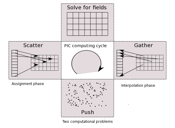
Figure 1: Phase of Particle-In-Cell algorithm

• Assignment Phase: for each particle $P$, assign the charge and current density into ${FEM}_{P}$. This step aims at collecting the total charge and current density induced by the particle.

• Field Solve Phase: using the charge and the current density found in the previous phase A, solve the Maxwell’s equations (time integration) through Finite Element Method to determine the electric and magnetic fields, $E$ and $B$.

• Interpolation Phase: for each particle $P$, use the value of $E$ and $B$ given by the Maxwell solver to interpolate the force value on $P$ at the particle’s actual position.

• Push Phase: update the position of each particle under the influence of the force determined in previous phase C.

This four tasks are performed at each time step of the simulation run. In the set of 2D test cases we are interested in, the Push step is often the more costly part. In the sequel, we will focus mainly on the parallelization and the optimization of the last phase (denoted D).

2.1 Particles distributions methods

Two methods are generally used in Particles-in-Cell code to distribute objects over parallel machine. These are the Lagrangian and the Eulerian decomposition methods. This nomenclature is presented by Hoshino et all [7] and presented with accuracy by David W. Walker in [13]. The reason why the two types of decompositions exist is due to the fact that a PIC code should consider to balance the load of the mesh firstly or of the particles firstly. The improvement of the particle distribution over processors reduces the cost of the push phase (D step); whereas a good distribution of finite elements enhances the performance of the field solver (B step).

The Eulerian method manages particles motion in displacing the particles among processors depending on their locations. Each processor handles a spatial sub-domain. Whenever particle changes of spatial sub-domain after a motion, this particle is pushed away from the processor and is sent to the processor owning the new sub-domain. A consequence of this method is that each processor manages all particles located inside a relatively small sub-domain. This motion of particles between the different processors constitutes an overhead in the Push step.

The Lagrangian method allows each processor to track the same set of particles during all the simulation on the whole spatial domain. Even if the particles are initially in a small area, they can travel far away from their first location depending of fields they traverse. In this case and after a while, it is likely that one processor can manage particles dispatched almost everywhere in the spatial domain. The main advantage of this method over Eulerian one is to limit the number of communication during the Push step because particles remain on the same processor. Nevertheless, the execution time needed by each processor to realize the Push step are often larger than in the Eulerian case because of a lack of cache phenomena. Hence, in the Eulerian case, each processor manages particles driven by a small set of discrete fields included in the processor sub-domain; whereas in the Lagrangian case, the processor’s set of particles can see all discrete fields of the spatial domain during the push step. Thus, there are much more spatial locality in the usage of field data in the Eulerian case than in the Lagrangian one. The cache memory usage is better in Eulerian decomposition as far as field data are concerned.

2.2 Dynamic load balancing strategies

In an Eulerian mapping, there are two kinds of method concerning the load balancing strategy. The first one, perhaps the most popular one, uses a static external graph partitioner like Metis or Scotch ([10, 12]). This external tool performs the partitioning of the mesh (and the spatial domain) at the beginning of the run, or can also be called off-line. This processing can have a relative high cost compared to the simulation runtime. It is possible, but not usual, to revise the partition during the simulation run, then using the partitioner multiple times per simulation. it may lead to a penalizing synchronization between processors.

We choose to study an alternate solution to perform load balancing. We would like to consider a dynamic strategy to partition the spatial domain over the processors that is revised during simulation. The main idea is to adapt the partition to a change of the macroscopic structure of particles.

In this case, the partition tool is integrated directly into the simulator. We expect this tool to be cheap in execution time and to be used frequently to adapt the partition to the dynamics of particles. We will focus hereafter on two methods implementing that kind of load balance strategy. The first one is a global partitioning method that considers the whole space domain and the computation cost (via a cost function) on each spatial unit. It is denoted URB (Unbalanced Recursive Bisection) in the literature. The second method we will look at, is known as ORB-H. This method prevents the synchronization of all processors during a dynamic mapping phase. This feature could be great when working on large scale platform, compared to the previous URB algorithm as we shall see afterward. In the two cases, URB and ORB-H, we choose to give to the partitioner an input rectangular shaped grid elements (for a domain in two dimensions). That means that each uncuttable rectangular grid element encompasses a set of finite elements and particles. We determine the responsible grid element for each element depending on the barycenter location of the element. The partitioner does not see finite elements nor particles but only the number of particles and finite elements encapsulated within a grid element. By the way, we avoid the difficulty of managing complex data-structure needed for finite elements and we avoid the computation of a partition of a general mesh. Furthermore, this approach facilitates the tuning of a partition based on rectangular sub-domains (see [2]). We will evaluate this kind of partitioning method.

As we already said, this study focuses on the parallel management and distribution of particles in a PIC code in order to mainly enhance the performance of the Push, Gather, Scatter steps and not on the Field solver. As a perspective, we wish to extend our results to the load balance of all steps of the code including the field solver. In order to do that, we will have to improve the cost function given to the partitioning algorithm to take into account the number of finite elements per grid element. Suppose we want to consider test cases that includes a costly Maxwell solver part; a small modification of the cost function will allow us to tackle this new configuration.

2.3 Grid elements

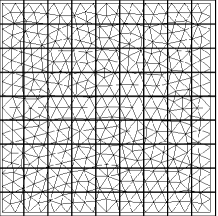
Figure 2: The initial grid element cutting

The figure 2 illustrates a sketched view of our spatial domain. A regular grid divides the domain in grid element. Each grid element has a rectangular shape and a fixed size defined as a parameter of the simulation. A grid element stores a set of finite elements (mesh information and field solver information) and particles. The first step of our simulation tool assigns each particle and finite element information to one grid element. We store also the belonging relation existing between particles and grid element. This relation is updated after each particle motion. The grid element sub-grid offers a way to simplify several mechanisms. First, the grid elements allow the parallel simulation to migrate finite elements and particles easily from one processor to the other (from the programming and software engineering point of view). The penalty in term of performance and partitioning quality is low if the number of grid elements per processor remains large. Second, the localization of particles is trivial for this kind of Cartesian sub-griding, which is a big advantage for a PIC code. Furthermore, one could derive a simple condition to detect when a particle leaves the processor sub-domain.

2.4 Initial partitioning

If the global space domain is a rectangle, one of the simplest mapping one can think of, is a homogeneous decomposition of rectangular sub-domains on processors. For the time being, we do not consider the number of particles per grid element as a constraint but simply distribute the same number of grid elements per processor. Here, we do not care about the cost function but propose a reference mapping for comparison purpose.

TYPE SUBDOMAIN
  INTEGER   pid                  ! processor id
  REAL*8    xmin,xmax,ymin,ymax  ! rectangle definition
  INTEGER   height               ! height of the node in the tree
END TYPE SUBDOMAIN

Figure 3: Data type used in the parallel domain decomposition

In several algorithm, the parallel domain decomposition is performed in building a tree. The data structure that constitutes a node of the tree is shown in figure 3. Each sub-domain is associated with a single processor. The field $pid$ contains the processor identity. The following fields define a rectangular area which corresponds to the sub-domain given to the processor. The integer $height$ stores the height of the cell in the tree of the hierarchical domain decomposition.

3 Different strategies for load balancing

Parallelisation of a PIC code relies to a large extent on the load balancing chosen and the partitioning scheme used. The partitioning scheme can be either hierarchical or non-hierarchical.

In a hierarchical partitioning, the mapping is derived from a tree representation of sub-domains. One can directly use the tree to adapt the mapping to minor changes of the load.

Hereafter, we will look at a few Recursive Coordinate Bisection (RCB) algorithms and an incremental partitioning solution known as the dimension exchange algorithm.

3.1 Simple geometric partitioning algorithm

The first algorithm we look at to perform the load balancing uses an improved version of the algorithm presented by Berger and Bokhari [2], known as Recursive Coordinate Bisection. The RCB algorithm divides each dimension alternatively in half part to obtain two sub-domains having approximately the same cost (using the user-defined cost function). The two halves are then further divided by applying the same process recursively. Finally, this algorithm provides a simple geometric decomposition for a number of processors equal to a power of two.

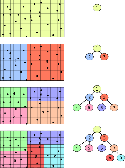
Figure 4: The URB partitioning strategy

This partitioning algorithm does not pay attention to the aspect ratio of the resulting sub-domains. If there is a large variation between dimensions of the domain, one of the two sub-domain boundaries can be very large compared to the other. Since the communication volume is related to the size of the sub-domain boundary (A and C phases), large aspect ratios are undesirable. The Unbalanced Recursive Bisection (URB) is an improvement of the previous partitioning method proposed by Jones and Plassmann [9]. They propose to try to minimize the aspect ratio and suppress the constraint of using power of two sub-domains. The main idea is to adjust the sub-domains size in respect to the estimated cost.

In our PIC code, we do not manage directly the finite elements but simply rectangular grid elements as we described previously. We used the load per cell to dispatch them on the different nodes.

The figure 4 illustrates an URB decomposition process. Firstly, we begin with a big cell containing all the processors and the whole spatial domain. At the start of this algorithm, the first cell contains all grid elements. Recursively, we divides each remaining cell of size ($n$,$m$) grid element into two parts in assigning to each new cell a distinct set of processors and distinct sub-domains. To divide the set of grid elements, we use the cost function to find the right cut.

We obtain two cells that have respectively the size of ($n-q$, $m$) and ($q$,$m$) (if the cut is in the first dimension). The choice of the q-size is determined using a simple method like the dichotomy to share the load with a fair and equitable strategy between the two cells. In a second step, the created cells are divided again in the other dimension. We choose the algorithm to perform the cut alternatively in each dimension (x or y). This last property of alternation allows one to obtain sub-domains with quite small perimeters. This choice is worthwhile because the volume of communication between different processors [2] is proportional to the sub-domain perimeters during scatter and gather phases. At the end of the recursion, the whole domain is split in balanced load parts. A tree structure is generated that stores each cut and finally the data structure of figure 3 in the leaves.

In our code, particles move at each iteration of the run between processors. Thereof it is necessary to regularly apply the partitioning algorithm to maintain a good load balance. From one iteration to the next, the partitioning algorithm we just described, can lead to very different mappings. Indeed, the algorithm does not try to keep or adjust the previous partition, but compute from scratch another partition. However, a big change of the partition can provoke a massive migration of objects between processors and can induce ta degradation of application performance. We will address the problem in the next section.

3.1.1 URB limited migration

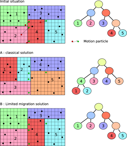
Figure 5: Illustration of the limited migration URB

We have designed a simple solution to constraint the load balancing process to use quite similar decomposition from one iteration to the other. Remind you that the tree structure is built during the partitioning process. We propose to modify a little bit the existing tree instead of building a new tree. Indeed, we adapt the algorithm to only authorize load exchange between cells belonging to the same branch of the tree, or, up to a maximum level of the partitioning tree. We set that only one frontier in each sub-domain is authorized to move during the URB algorithm. Consequently, we stop the risk of a global modification of the partition, and then we limit the migration of data between processors. Nevertheless, if particle motions are large enough, and if the global load balance becomes not so good, this version of load balancing that preserve locality could be inadequate. If ever this unusual configuration happens, it would be useful to call the standard URB load balancing to correct the imbalance.

The difference between the classical URB and the modified version is shown in the figure 5. The $A$ case corresponds the classical URB algorithm applied after a migration of the particles. One can see a large change of the domain decomposition. Many grid elements and associated particles have to migrate on their new processors. In opposite, the limited migration URB restrains the modifications of the tree to happen in nodes higher than the third level. The result is that the new tree is close to the old one. Only the boundaries of three sub-domains are moving.

Finally, this new version of the algorithm fills our first objectives. A remaining problem is about the synchronization still required between all processors during the partitioning algorithm. It is a bad point for large parallel platforms. The tree is unique for all processors and obtained with the knowing of the loads computed in each grid element. This adds a communication step that can penalize the global performance of the application. In the sequel, we propose a local algorithm that computes dynamically a partitioning avoiding global synchronization.

3.2 A diffusion algorithm for the load balancing

A communication bottleneck is a major drawback for a parallel algorithm. The previous algorithms need a gather step to share information and require a synchronization. All processors are waiting to each other, and in worse cases, the time loss could be significant. A simple way to overcome this bottleneck is to avoid the global communication and replace it with communications only towards neighboring processors. For load balancing purpose, Cybenko [6] described an incremental algorithm that uses the first order diffusion equation. At each simulation iteration, this diffusion algorithm proceeds to local exchanges of load between closer processors. It converges asymptotically (for an infinite number of iterations) towards a uniform load balance. Many improvements of this algorithm have been published and we highlight the following papers [8, 14] for the practical description given.

$$w^{t+1}_{i}=w^{t}_{i}+\sum_{j}{\alpha_{i,j}(w^{t}_{j}-w^{t}_{i})}+\eta^{t+1}_{i}-c_{i}$$ (1)

The algorithm is based on the diffusion equation (1) that is able to estimate the diffusion of the load between processors in the framework of dynamic load balancing. In the previous formula, $w^{t}_{i}$ corresponds to the load of processor $i$ at time $t$. $\eta^{t+1}_{i}$ is the load who will be created on the processor $i$ at time $t$. The consumed load by a processor during an iteration is $c_{i}$. In our application, the $c_{\star}$ constant is always zero because the work to perform is the same at each time step. Work does not diminish along time dimension.

In this algorithm, all processors can exchange load at each iteration. But, sometimes, it is not possible to exchange load easily without paying large communication costs. At the utmost, we can even choose to impose that a node $i$ can only exchange load with one node $j$ at an iteration $t$ in order to reduce amount of communication. This solution is proposed by Cybenko [6] and this algorithm is known as the diffusion exchange algorithm. This algorithm use processors two by two to obtain the asymptotic stability state [8].

For our simulation, we fix the parameter $\alpha_{*,*}$ to $1/2$ uniformly and $\eta^{*}_{*}$ to $0$. The formula 1 becomes :

$$w^{t+1}_{i}=w^{t}_{i}+\frac{1}{2}(w^{t}_{j}-w^{t}_{i})$$ (2)

The scheme of figure 6 shows a 4x4 grid of processors. Capability of load exchange is sketched by a link between two nodes. Using a colored graph, it is easy to deduce at the iteration $t$ which processors exchange load. The figure 6 describes a domain in two dimensions.

In this figure, we can classify the processors into two different sets. The first set, composed by the processor place on the middle of the domain, have all of its communication channels with the other processors. In the context of the figure 6, this class contains the processors 6,7,10 and 11. For example, the processor 6 can exchange data with the processor 5, when $mod(it_{number},4)=1$, with the processor 7, when $mod(it_{number},4)=2$, and with the processor 2 and 10 in the corresponding case. The other case of processor (the number 1,2,3,4,5,8,9,12,13,14,15 and 16) has the same behavior as the first class usually. But, in some cases, as this processor have not all of the channels of communication, the results of $mod(it_{number},4)$ give a choice of channels not available on the processor (like the channel 1 for the processor 1). In this case, this processor does not participate at the load balancing step for this iteration.

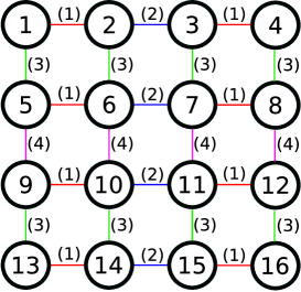
Figure 6: Coloured grid 4x4

A specific design is needed to take into account the distributed feature of this algorithm. As we already have described in the previous section, the first partitioning strategy choice is not very useful to exchange load between different neighbors. The only allowed choice is the cell in the same level or in the same branch on the partitioning tree. As we want to have more possibilities to exchange load, we have preferred to use an another strategy of partitioning: the ORB-H strategy proposed by M. Campbell, A. Carmona and W. Walker in [4, 5]. This strategy divides each different dimension separately and does not need the use of another data structure to store the global scheme of the partitioning. The figure 7 presents the ORB-H decomposition for the example already presented in 4.

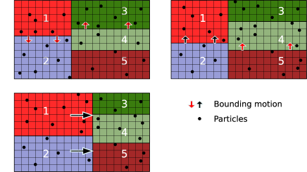
Figure 7: The -H partitioning strategy

The scheme 7 shows that all the borders are not independent as for the URB partitioning. The exchange of load cannot be realized in all the dimensions at a time and only the last partitioned dimension can be easily used for the load balancing process (in 1D). In practice, for our application, each node has the choice between at most two nodes at each iteration to proceed to a load exchange.

The work domain is the same as in the previous case. The domain is 2D and use a first regular decomposition of grid elements. The initializing process is realized in two steps. First, the algorithm divides the domain in equally sized parts using only one dimension load balancing. The choice of the first dimension dividing the global domain is important and must be chosen adequately with the particle motions. At the next iteration, the process divides the second dimension in equivalent load parts.

During the global process, particles moves in space and a situation of load imbalance could appear. In the previous algorithm, this detection must be solved by a global process of load balancing involving all nodes. In the case of a distributed algorithm, only the node affected by this situation try to solve it with its closest neighbors.

The diffusion exchange algorithm uses the following principles :

• one node can exchange its load with only one neighbor in the same sub iteration of load balancing,

• the volume of the load exchange is given by the previous formula 1. In our case, the volume correspond to the number of grid elements that can migrate between two nodes.

With the simple scheme (figure 7), the exchange of load is possible between the node 1 and 2, 3 and 4. The node 5 does not perform load balancing step at this first iteration. At the next iteration of load balancing, the exchange of data uses the same configuration for the first column, but for the second, only the 4 and 5 exchange load. And less frequently the column of the cells 1 and 2 could exchange load with column of the cells 3,4 and 5. We have implemented a predictive method to do the choice of a couple of nodes exchanging their load using the parity of the node. The implementation of this algorithm uses the same structure than the URB algorithm.

4 Results

4.1 Numerical experiments

We have tested our algorithms in many situations considering few parameters variation. To limit the number of cases to run, we have fixed a limited number of parameters as the number of particles (eighty millions), the number of iteration to be computed (one thousand) and the type of test case. We have studied the case of the "Two stream instability" [3] in two dimensions. This case is a periodic case, so the number of particles, equivalent to the cost function load for us in this study, is the same along the evaluation, there is no loss of particles.

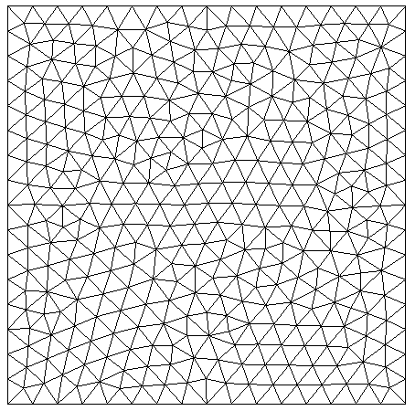
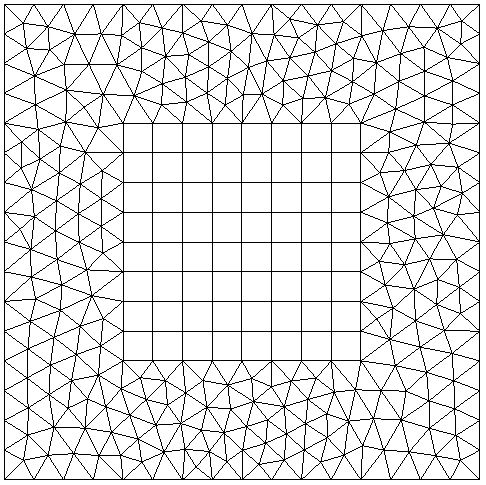
Figure 8: Regular mesh (left), unstructured mesh (middle) and hybrid mesh (right)

We have tested our simulation using two distinct types of mesh, quadrangles and unstructured mesh. A view of this two types of mesh are shown in the figure 8.

Parameters used to study the efficient of different types of load balancing algorithms are the following. We have tested the variation of the number of vertices and edges of the used mesh, and the type of mesh (triangles or quads). We have used the dedicated high-performance facilities of the University of Strasbourg. This cluster has 512 processors dispatched within in 64 bi-processor nodes (Intel Opteron 2384).

4.2 Dimensionnal study for the two kinds of mesh

A first comparison has the objective to show the behavior of several algorithms depending on the mesh size. This test uses the common setting with a grid of $4\times 8$ processors. The two evolving parameters are the type of mesh, and its size ($16\times 16$, up to $128\times 128$).

	Regular mesh		Unstructured mesh
	Nb of quads	time	Nb of triangles	time
16x16	256	7847 s	696	7665 s
32x32	1024	8076 s	2730	7575 s
64x64	4096	8417 s	10574	7830 s
128x128	16384	8041 s	35930	8568 s

Table 1: Dimensional study for the two kinds of mesh

The results and the sizes of the meshes are presented in the table 1. It shows the very good behaviour of our implementation depending on the evolution of the size (i.e. increasing the mesh size does not induce an increase of the execution time which is mainly prescribed by the number of particles). Indeed, the global time of a simulation is relatively independent of the mesh size because the time used in the field solve phase (see figure 1) is small, around five to ten percent of the global time of an iteration.

4.3 Comparison between different methods for particles management

	Lagrangian	Eulerian
	(P1)	(P3)
static (1)	21175s	8325 s
static* (2)	22519s	8948 s
URB	9212s	8684 s
URB-limited	9682s	8376 s
ORB-H	9174s	8568 s

Table 2: Global evaluation for particles push methods

This comparison aims at showing the difference between the two methods (Lagrangian and Eulerian) depending on the partitioning algorithm. As it is shown in the section 2.1, the main difference between these two methods is that the spatial locality effect in the cache can be favored. The particles that are close to each other use the same data of the elements which can favor cache effects. There is also a benefit brought by avoiding particle migrations. This test uses the two partitioning methods described previously and illustrated in the figure 9.

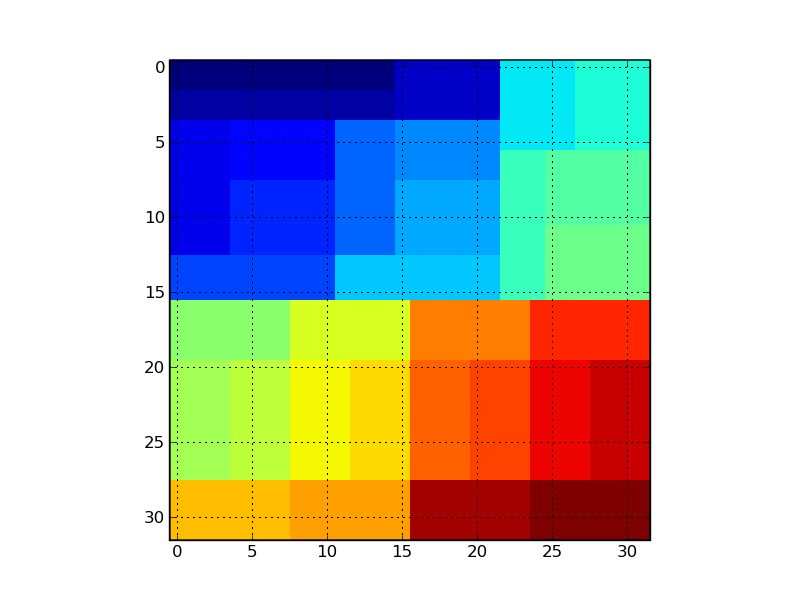
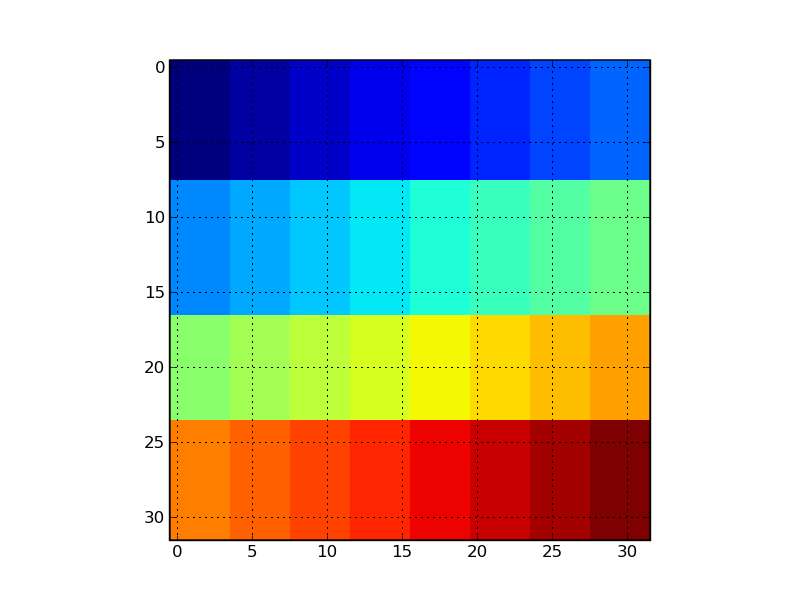
Figure 9: Comparison between URB (on the left) and ORB-H (on the right) dynamic load balancing process. Each color represents a processor’s domain.

To show main differences between these two methods, we have compared the difference on the global time for one simulation and the time needed for one iteration during the simulation for each load balancing algorithm for static and dynamic versions. The table 2 presents the results of the global computation time for each case of the study. The main finding is about the differences between the static and the dynamic load balancing. In the Eulerian case, the difference is not existent because this method of particles motion allow the localized push of particles within each processor. For the Lagrangian method, the static method are very penalizing for the particles motion cost. In this case, each processor keep the same set of particles during the whole simulation run. After many iteration of calculus, each processor manages particles dispersed over the whole simulation domain. This context of calculus does not facilitate the optimization of the execution and induces an increase by a factor two at least on the global time of the simulation.

Figure 10: Importance of the method for particle motions

The figure 10 presents the computation time for each iteration in the previous context. In the two cases, static and dynamic, the Eulerian method (P3) is more efficient compared to the Lagrangian method (P1). This optimization is clearly visible for the static case. Indeed, in the dynamic case, particles are re-localized and re-distributed at each load balancing step.

The improvement brought by the Eulerian dynamic method is around 15% on the execution time compared to Eulerian static.

4.4 Comparison between static and dynamic load balancing for the two types of mesh

	static	URB	ORB-H
	URB	“limited”
Regular	7921 s	8250 s	8041 s
Unstructured	8325 s	8376 s	8568 s
Hybrid	7651 s	7907 s	8328 s

Table 3: Global evaluation for the two families of mesh (using a $128\times 128$ mesh)

This test shows the difference of performance of our simulator using the two types of mesh. This benchmark uses the common configuration like all the previous benchmarks. We have choose to do this bench with a mesh size of $128\times 128$ and we have using the Eulerian distribution method to manage particles. The regular mesh is compound of 16641 vertices and 16384 quads. Respectively, the unstructured mesh is compound of 18222 vertices and 35930 triangles. The results are detailed in the table 3. In conclusion to this, we can say that the difference of performance is existent but not very large. Indeed, the maximum difference between two execution times is about ten percent. This small difference of performance between these two types of mesh exists because most of the time consumed within one iteration is consumed by the push particles function (neighborhood management and communications represents less than 10 percents).

Conclusion

We have studied in this work several algorithms of load balancing for a PIC code using static or dynamic partitioning. We have shown that the dynamic management is a key point to optimize the overall performance of the application. But, we have not shown a large difference between the load balancing algorithms under investigation. Indeed, the measured times remain close to each other for the considered algorithms. The localization of the exchange with the limited version of the URB partitioning or using the ORB-H have not led to the improvement we hoped. Two facts can explain this. The first is about our developments of parallel algorithms. There are some points of synchronization we should remove that are killing performance. The second point is that the use cases which are maybe not well designed to evaluate the different load balancing algorithms (not enough particles moving around). The perspectives are, first, to find a another use case to evaluated with accuracy the load balancing algorithms and second, to study the load balancing for this PIC code over a 3D mesh instead of a 2D one.

References

- [1] Hyam Abboud, Sébastien Jund, Stéphanie Salmon, Eric Sonnendrücker, and Hamdi Zorgati. Two-scale simulation of Maxwell’s equations. In EDP Sciences, editor, ESAIM: Proceedings CEMRACS 2005 - Computational Aeroacoustics and Computational Fluid Dynamics in Turbulent Flows Marseille, France, July 18 - August 26, 2005, Volume 16, pages 211–223. EDP Sciences, 02 2007.
- [2] M. J. Berger and S. H. Bokhari. A partitioning strategy for nonuniform problems on multiprocessors. IEEE Trans. Comput., 36(5):570–580, 1987.
- [3] Nicolas Besse, Francis Filbet, Michaël Gutnic, Ioana Paun, and Eric Sonnendrücker. An adaptive numerical method for the Vlasov equation based on a multiresolution analysis. In Numerical mathematics and advanced applications. Proceedings of ENUMATH 2001, the 4th European conference, Ischia, July 2001., pages 437–446. Springer, 2003.
- [4] P.M. Campbell, E.A. Carmona, and D.W. Walker. Hierarchical domain decomposition with unitary load balancing for electromagnetic particle-in-cell codes. Distributed Memory Computing Conference, 1990., Proceedings of the Fifth, 2:943–950, Apr 1990.
- [5] Edward A. Carmona and Leon J. Chandler. On parallel pic versatility and the structure of parallel pic approaches. Concurrency - Practice and Experience, 9(12):1377–1405, 1997.
- [6] G. Cybenko. Dynamic load balancing for distributed memory multiprocessors. J. Parallel Distrib. Comput., 7(2):279–301, 1989.
- [7] Tsutomu Hoshino, Robert Hiromoto, Satoshi Sekiguchi, and S. Majima. Mapping schemes of the particle-in-cell method implemented on the pax computer. Parallel Computing, 9(1):53–75, 1988.
- [8] Emmanuel Jeannot and Flavien Vernier. A practical approach of diffusion load balancing algorithms. In Wolfgang E. Nagel, Wolfgang V. Walter, and Wolfgang Lehner, editors, Euro-Par, volume 4128 of Lecture Notes in Computer Science, pages 211–221. Springer, 2006.
- [9] Mark T. Jones and Paul E. Plassmann. Paper submitted to: Third national symposium on large-scale structural analysis for high-performance computers and workstations computational results for parallel unstructured mesh computations.
- [10] George Karypis and Vipin Kumar. Metis - unstructured graph partitioning and sparse matrix ordering system, version 2.0. Technical report, 1995.
- [11] C. Othmer, K. H. Glassmeier, U. Motschmann, J. Schule, and Ch. Frick. Numerical simulation of ion thruster-induced plasma dynamics – the model and initial results. Advances in Space Research, 29(9):1357 – 1362, 2002.
- [12] François Pellegrini. Native mesh ordering with scotch 4.0, 2003.
- [13] David W. Walker. Characterizing the parallel performance of a large-scale, particle-in-cell plasma simulation code,. Concurrency: Practice and Experience, 2(4):257–288, 1990.
- [14] Jerrell Watts and Stephen Taylor. A practical approach to dynamic load balancing. IEEE Transactions on Parallel and Distributed Systems, 9(3):235–248, 1998.