Location of the spectrum of Kronecker random matrices

Abstract

Abstract: For a general class of large non-Hermitian random block matrices ${\bm{X}}$ we prove that there are no eigenvalues away from a deterministic set with very high probability. This set is obtained from the Dyson equation of the Hermitization of ${\bm{X}}$ as the self-consistent approximation of the pseudospectrum. We demonstrate that the analysis of the matrix Dyson equation from [3] offers a unified treatment of many structured matrix ensembles.

Keywords: Outliers, block matrices, local law, non-Hermitian random matrix, self-consistent pseudospectrum
AMS Subject Classification: 60B20, 15B52

1 Introduction

Large random matrices tend to exhibit deterministic patterns due to the cumulative effects of many independent random degrees of freedom. The Wigner semicircle law [33] describes the deterministic limit of the empirical density of eigenvalues of Wigner matrices, i.e., Hermitian random matrices with i.i.d. entries (modulo the Hermitian symmetry). For non-Hermitian matrices with i.i.d. entries, the limiting density is Girko’s circular law, i.e., the uniform distribution in a disc centered around zero in the complex plane, see [16] for a review.

For more complicated ensembles, no simple formula exists for the limiting behavior, but second order perturbation theory predicts that it may be obtained from the solution to a nonlinear equation, called the Dyson equation. While simplified forms of the Dyson equation are present in practically every work on random matrices, its full scope has only recently been analyzed systematically, see [3]. In fact, the proper Dyson equation describes not only the density of states but the entire resolvent of the random matrix. Treating it as a genuine matrix equation unifies many previous works that were specific to certain structures imposed on the random matrix. These additional structures often masked a fundamental property of the Dyson equation, its stability against small perturbations, that plays a key role in proving the expected limit theorems, also called global laws. Girko’s monograph [24] is the most systematic collection of many possible ensembles, yet it analyzes them on a case by case basis.

In this paper, using the setup of the matrix Dyson equation (MDE) from [3], we demonstrate a unified treatment for a large class of random matrix ensembles that contain or generalize many of Girko’s models. For brevity, we focus only on two basic problems: (i) obtaining the global law and (ii) locating the spectrum. The global law, typically formulated as a weak convergence of linear statistics of the eigenvalues, describes only the overwhelming majority of the eigenvalues. Even local versions of this limit theorem, commonly called local laws (see e.g. [21, 17, 6] and references therein) are typically not sensitive to individual eigenvalues and they do not exclude that a few eigenvalues are located far away from the support of the density of states.

Extreme eigenvalues have nevertheless been controlled in some simple cases. In particular, for the i.i.d. cases, it is known that with a very high probability all eigenvalues lie in an $\varepsilon$-neighborhood of the support of the density of states. These results can be proven with the moment method, see [9, Theorem 2.1.22] for the Hermitian (Wigner) case, and [23] for the non-Hermitian i.i.d. case; see also [11, 12] for the optimal moment condition. More generally, norms of polynomials in large independent random matrices can be computed via free probability; for GUE or GOE Gaussian matrices it was achieved in [25] and generalized to polynomials of general Wigner and Wishart type matrices in [8, 18]. These results have been extended recently to polynomials that include deterministic matrices with the goal of studying outliers, see [13] and references therein.

All these works concern Hermitian matrices either directly or indirectly by considering quantities, such as norms of non-Hermitian polynomials, that can be deduced from related Hermitian problems. For general Hermitian random matrices, the density of states may be supported on several intervals. In this situation, excluding eigenvalues outside of the convex hull of this support is typically easier than excluding possible eigenvalues lying inside the gaps of the support. This latter problem, however, is especially important for studying the spectrum of non-Hermitian random matrices ${\bm{X}}$, since the eigenvalues of ${\bm{X}}$ around a complex parameter $\zeta$ can be understood by studying the spectrum of the Hermitized matrix

$$\bm{H}^{\zeta}=\begin{pmatrix}0&{\bm{X}}-\zeta\cr{\bm{X}}^{*}-\bar{\zeta}&0\end{pmatrix}$$ (1.1)

around 0. Note that for $\zeta\in\mathbb{C}$ away from the spectrum of ${\bm{X}}$, zero will typically fall inside a gap of the spectrum of $\bm{H}^{\zeta}$ by its symmetry.

In this paper, we consider a very general class of structured block matrices ${\bm{X}}$ that we call Kronecker random matrices since their structure is reminiscent to the Kronecker product of matrices. They have $L\times L$ large blocks and each block consists of a linear combination of random $N\times N$ matrices with centered, independent, not necessarily identically distributed entries; see (2.1) later for the precise definition. We will keep $L$ fixed and let $N$ tend to infinity. The matrix $\bm{\mathrm{X}}$ has a correlation structure that stems from allowing the same $N\times N$ matrix to appear in different blocks. This introduces an arbitrary linear dependence among the blocks, while keeping independence inside the blocks. The dependence is thus described by $L\times L$ deterministic structure matrices.

Kronecker random ensembles occur in many real-world applications of random matrix theory, especially in evolution of ecosystems [26] and neural networks [30]. These evolutions are described by a large system of ODE’s with random coefficients and the spectral radius of the coefficient matrix determines the long time stability, see [29] for the original idea. More recent results are found in [1, 4, 5] and references therein. The ensemble we study here is even more general as it allows for linear dependence among the blocks described by arbitrary structure matrices. This level of generality is essential for another application; to study spectral properties of polynomials of random matrices. These are often studied via the “linearization trick” and the linearized matrix is exactly a Kronecker random matrix. This application is presented in [19], where the results of the current paper are directly used.

We present general results that exclude eigenvalues of Kronecker random matrices away from a deterministic set ${\mathbb{D}}$ with a very high probability. The set ${\mathbb{D}}$ is determined by solving the self-consistent Dyson equation. In the Hermitian case, ${\mathbb{D}}$ is the self-consistent spectrum defined as the support of the self-consistent density of states $\rho$ which is defined as the imaginary part of the solution to the Dyson equation when restricted to the real line. We also address the general non-Hermitian setup, where the eigenvalues are not confined to the real line. In this case, the set ${\mathbb{D}}={\mathbb{D}}_{\varepsilon}$ contains an additional cutoff parameter $\varepsilon$ and it is the self-consistent $\varepsilon$-pseudospectrum, given via the Dyson equation for the Hermitized problem $\bm{H}^{\zeta}$, see (2.7) later. The $\varepsilon\to 0$ limit of the sets ${\mathbb{D}}_{\varepsilon}$ is expected not only to contain but to coincide with the support of the density of states in the non-Hermitian case as well, but this has been proven only in some special cases. We provide numerical examples to support this conjecture.

We point out that the global law and the location of the spectrum for $A+X$, where $X$ is an i.i.d. centered random matrix and $A$ is a general deterministic matrix (so-called deformed ensembles), have been extensively studied, see [10, 14, 15, 31, 32]. For more references, we refer to the review [16]. In contrast to these papers, the main focus of our work is to allow for general (not necessarily identical) distributions of the matrix elements.

In this paper, we first study arbitrary Hermitian Kronecker matrices $\bm{H}$; the Hermitization $\bm{H}^{\zeta}$ of a general Kronecker matrix is itself a Kronecker matrix and therefore just a special case. Our first result is the global law, i.e., we show that the empirical density of states of $\bm{H}$ is asymptotically given by the self-consistent density of states $\rho$ determined by the Dyson equation. We then also prove an optimal local law for spectral parameters away from the instabilities of the Dyson equation. The Dyson equation for Kronecker matrices is a system of $2N$ nonlinear equations for $L\times L$ matrices, see (2.6) later. In case of identical distribution of the entries within each $N\times N$ matrix, the system reduces to a single equation for a $2L\times 2L$ matrix – a computationally feasible problem. This analysis provides not only the limiting density of states but also a full understanding of the resolvent for spectral parameters $z$ very close to the real line, down to scales $\operatorname{Im}z\gg 1/N$. Although the optimal local law down to scales $\operatorname{Im}z\gg 1/N$ cannot capture individual eigenvalues inside the support of $\rho$, the key point is that outside of this support a stronger estimate in the local law may be proven that actually detects individual eigenvalues, or rather lack thereof. This observation has been used for simpler models before, in particular [21, Theorem 2.3] already contained this stronger form of the local semicircle law for generalized Wigner matrices, see also [2] for Wigner-type matrices, [7] for Gram matrices and [20] for correlated matrices with a uniform lower bound on the variances. In particular, by running the stability analysis twice, this allows for an extension of the local law for any $\operatorname{Im}z>0$ outside of the support of $\rho$.

Finally, applying the local law to the Hermitization $\bm{H}^{\zeta}$ of a non-Hermitian Kronecker matrix ${\bm{X}}$, we translate local spectral information on $\bm{H}^{\zeta}$ around 0 into information about the location of the spectrum of ${\bm{X}}$. This is possible since $\zeta\in\mbox{Spec}({\bm{X}})$ if and only if $0\in\mbox{Spec}(\bm{H}^{\zeta})$. In practice, we give a good approximation to the $\varepsilon$-pseudospectrum of ${\bm{X}}$ by considering the set of those $\zeta$ values in $\mathbb{C}$ for which 0 is at least $\varepsilon$ distance away from the support of the self-consistent density of states for $\bm{H}^{\zeta}$.

In the main part of the paper, we give a short, self-contained proof that directly aims at locating the Hermitian spectrum under the weakest conditions for the most general setup. We split the proof into two well-separated parts; a random and a deterministic one. In Section 4 and 5 as well as Appendix B we give a model-independent probabilistic proof of the main technical result, the local law (Theorem 4.7 and Lemma B.1), assuming only two explicit conditions, boundedness and stability, on the solution of the Dyson equation that can be checked separately for concrete models. In Section 3.2 we prove that these two conditions are satisfied for Kronecker matrices away from the self-consistent spectrum. The key inputs behind the stability are (i) a matrix version of the Perron-Frobenius theorem and (ii) a sophisticated symmetrization procedure that is much more transparent in the matrix formulation. In particular, the global law is an immediate consequence of this approach. Moreover, the analysis reveals that outside of the spectrum the stability holds without any lower bound on the variances, in contrast to local laws inside the bulk spectrum that typically require some non-degeneracy condition on the matrix of variances.

We stress that only the first part involves randomness and we follow the Schur complement method and concentration estimates for linear and quadratic functionals of independent random variables. Alternatively, we could have used the cumulant expansion method that is typically better suited for ensembles with correlation [20]. We opted for the former path to demonstrate that correlations stemming from the block structure can still be handled with the more direct Schur complement method as long as the non-commutativity of the $L\times L$ structure matrices is properly taken into account. Utilizing a powerful tensor matrix structure generated by the correlations between blocks resolves this issue automatically.

Acknowledgement

The authors are grateful to David Renfrew for several discussions and for calling their attention to references on applications of non-Hermitian models.

1.1 Notation

Owing to the tensor product structure of Kronecker random matrices (see Definition 2.1 below), we need to introduce different spaces of matrices. In order to make the notation more transparent to the reader, we collect the conventions used on these spaces in this subsection.

For $K,N\in\mathbb{N}$, we will consider the spaces $\mathbb{C}^{K\times K}$, $(\mathbb{C}^{K\times K})^{N}$ and $\mathbb{C}^{K\times K}\otimes\mathbb{C}^{N\times N}$, i.e., we consider $K\times K$ matrices, $N$-vectors of $K\times K$ matrices and $N\times N$ matrices with $K\times K$ matrices as entries. For brevity, we denote ${{\mathcal{M}}}\mathrel{\vbox{\hbox{\scriptsize.}\hbox{\scriptsize.}}}=\mathbb{C}^{K\times K}\otimes\mathbb{C}^{N\times N}$. Elements of $\mathbb{C}^{K\times K}$ are usually denoted by small roman letters, elements of $(\mathbb{C}^{K\times K})^{N}$ by small boldface roman letters and elements of ${{\mathcal{M}}}$ by capitalized boldface roman letters.

For $\alpha\in\mathbb{C}^{K\times K}$, we denote by $\lvert\alpha\rvert$ the matrix norm of $\alpha$ induced by the Euclidean distance on $\mathbb{C}^{K}$. Moreover, we define two different norms on the $N$-vectors of $K\times K$ matrices. For any $\bm{r}=(r_{1},\ldots,r_{N})\in(\mathbb{C}^{K\times K})^{N}$ we define $\lVert\bm{r}\rVert\mathrel{\vbox{\hbox{\scriptsize.}\hbox{\scriptsize.}}}=\max_{i=1}^{N}\lvert r_{i}\rvert$, and

$$\lVert\bm{r}\rVert_{\mathrm{hs}}^{2}\mathrel{\vbox{\hbox{\scriptsize.}\hbox{\scriptsize.}}}=\frac{1}{NK}\sum_{i=1}^{N}\operatorname{Tr}(r_{i}^{*}r_{i}).$$ (1.2)

These are the analogues of the maximum norm and the Euclidean norm for vectors in $\mathbb{C}^{N}$ which corresponds to $K=1$. Note that $\lVert\bm{r}\rVert_{\mathrm{hs}}\leq\lVert\bm{r}\rVert$.

For any function $f\colon U\to\mathbb{C}^{K\times K}$ from $U\subset\mathbb{C}^{K\times K}$ to $\mathbb{C}^{K\times K}$, we lift $f$ to $U^{N}$ by defining $f(\bm{r})\in(\mathbb{C}^{K\times K})^{N}$ entrywise for any $\bm{r}=(r_{1},\ldots,r_{N})\in U^{N}\subset(\mathbb{C}^{K\times K})^{N}$, i.e.,

$$f(\bm{r})\mathrel{\vbox{\hbox{\scriptsize.}\hbox{\scriptsize.}}}=(f(r_{1}),\ldots,f(r_{N})).$$ (1.3)

We will in particular apply this definition for $f$ being the matrix inversion map and the imaginary part. Moreover, for $\bm{x}=(x_{1},\ldots,x_{N})$, $\bm{y}=(y_{1},\ldots,y_{N})\in(\mathbb{C}^{K\times K})^{N}$ we introduce their entrywise product $\bm{x}\bm{y}\in(\mathbb{C}^{K\times K})^{N}$ through

$$\bm{x}\bm{y}\mathrel{\vbox{\hbox{\scriptsize.}\hbox{\scriptsize.}}}=(x_{1}y_{1},\ldots,x_{N}y_{N})\in(\mathbb{C}^{K\times K})^{N}.$$ (1.4)

Note that for $K\neq 1$, in general, $\bm{x}\bm{y}\neq\bm{y}\bm{x}$.

If $a\in\mathbb{C}^{K\times K}$ or $\bm{A}\in{{\mathcal{M}}}$ are positive semidefinite matrices, then we write $a\geq 0$ or $\bm{A}\geq 0$, respectively. Similarly, for $\bm{a}\in(\mathbb{C}^{K\times K})^{N}$, we write $\bm{a}\geq 0$ to indicate that all components of $\bm{a}$ are positive semidefinite matrices in $\mathbb{C}^{K\times K}$. The identity matrix in $\mathbb{C}^{K\times K}$ and ${{\mathcal{M}}}$ is denoted by $\mathds{1}$.

We also use two norms on ${{\mathcal{M}}}$. These are the operator norm $\lVert{\,\cdot\,}\rVert_{2}$ induced by the Euclidean distance on $\mathbb{C}^{KN}\cong\mathbb{C}^{K}\otimes\mathbb{C}^{N}$ and the norm $\lVert{\,\cdot\,}\rVert_{\mathrm{hs}}$ induced by the scalar product $\langle{{\,\cdot\,}}\mspace{2.0mu},{{\,\cdot\,}}\rangle$ on ${{\mathcal{M}}}$ defined through

$$\langle{{\bm{R}}}\mspace{2.0mu},{{\bm{T}}}\rangle\mathrel{\vbox{\hbox{\scriptsize.}\hbox{\scriptsize.}}}=\frac{1}{NK}\operatorname{Tr}\left({\bm{R}}^{*}{\bm{T}}\right),\qquad\lVert{\bm{R}}\rVert_{\mathrm{hs}}\mathrel{\vbox{\hbox{\scriptsize.}\hbox{\scriptsize.}}}=\sqrt{\langle{{\bm{R}}}\mspace{2.0mu},{{\bm{R}}}\rangle},$$ (1.5)

for ${\bm{R}},{\bm{T}}\in{{\mathcal{M}}}$. In particular, all orthogonality statements on ${{\mathcal{M}}}$ are understood with respect to this scalar product. Furthermore, we introduce $\langle{\bm{R}}\rangle\mathrel{\vbox{\hbox{\scriptsize.}\hbox{\scriptsize.}}}=\langle{\mathds{1}}\mspace{2.0mu},{{\bm{R}}}\rangle$, the normalized trace for ${\bm{R}}\in{{\mathcal{M}}}$.

We also consider linear maps on $(\mathbb{C}^{K\times K})^{N}$ and ${{\mathcal{M}}}$, respectively. We follow the convention that the symbols ${\mathscr{S}}$, ${\mathscr{L}}$ and $\mathscr{T}$ label linear maps $(\mathbb{C}^{K\times K})^{N}\to(\mathbb{C}^{K\times K})^{N}$ and $\bm{\mathcal{S}}$, $\bm{\mathcal{L}}$ or $\bm{\mathcal{T}}$ denote linear maps ${{\mathcal{M}}}\to{{\mathcal{M}}}$. The symbol $\mathrm{Id}$ refers to the identity map on ${{\mathcal{M}}}$. For any linear map $\mathscr{T}\colon(\mathbb{C}^{K\times K})^{N}\to(\mathbb{C}^{K\times K})^{N}$, let $\lVert\mathscr{T}\rVert$ denote the operator norm of $\mathscr{T}$ induced by $\lVert{\,\cdot\,}\rVert$ and let $\lVert\mathscr{T}\rVert_{\mathrm{sp}}$ denote the operator norm induced by $\lVert{\,\cdot\,}\rVert_{\mathrm{hs}}$. Similarly, for a linear map $\bm{\mathcal{T}}\colon{{\mathcal{M}}}\to{{\mathcal{M}}}$, we write $\lVert\bm{\mathcal{T}}\rVert$ for the operator norm induced by $\lVert{\,\cdot\,}\rVert_{2}$ on ${{\mathcal{M}}}$ and $\lVert\bm{\mathcal{T}}\rVert_{\mathrm{sp}}$ for its operator norm induced by $\lVert{\,\cdot\,}\rVert_{\mathrm{hs}}$ on ${{\mathcal{M}}}$.

We use the notation $[n]\mathrel{\vbox{\hbox{\scriptsize.}\hbox{\scriptsize.}}}=\{1,\ldots,n\}$ for $n\in\mathbb{N}$. For $i,j\in[N]$, we introduce the matrix $E_{ij}\in\mathbb{C}^{N\times N}$ which has a one at its $(i,j)$ entry and only zeros otherwise, i.e.,

$$E_{ij}\mathrel{\vbox{\hbox{\scriptsize.}\hbox{\scriptsize.}}}=(\delta_{ik}\delta_{jl})_{k,l=1}^{N}.$$ (1.6)

For $i,j\in[N]$, the linear map $P_{ij}\colon{{\mathcal{M}}}\to\mathbb{C}^{K\times K}$ is defined through

$$P_{ij}{\bm{R}}=r_{ij},$$ (1.7)

for any ${\bm{R}}=\sum_{i,j=1}^{N}r_{ij}\otimes E_{ij}\in{{\mathcal{M}}}$ with $r_{ij}\in\mathbb{C}^{K\times K}$.

2 Main results

Our main object of study are Kronecker random matrices which we define first. To that end, we recall the definition of $E_{ij}$ from (1.6).

Definition 2.1 (Kronecker random matrix).

A random matrix ${\bm{X}}\in\mathbb{C}^{L\times L}\otimes\mathbb{C}^{N\times N}$ is called Kronecker random matrix if it is of the form

$${\bm{X}}=\sum_{\mu=1}^{\ell}\widetilde{\alpha}_{\mu}\otimes X_{\mu}+\sum_{\nu=1}^{\ell}(\widetilde{\beta}_{\nu}\otimes Y_{\nu}+\widetilde{\gamma}_{\nu}\otimes Y_{\nu}^{*})+\sum_{i=1}^{N}\widetilde{a}_{i}\otimes E_{ii},\qquad\ell\in\mathbb{N},$$ (2.1)

where $X_{\mu}=X_{\mu}^{*}\in\mathbb{C}^{N\times N}$ are Hermitian random matrices with centered independent entries (up to the Hermitian symmetry) and $Y_{\nu}\in\mathbb{C}^{N\times N}$ are random matrices with centered independent entries; furthermore $X_{1},\ldots,X_{\ell},Y_{1},\ldots,Y_{\ell}$ are independent. The “coefficient” matrices $\widetilde{\alpha}_{\mu},\widetilde{\beta}_{\nu},\widetilde{\gamma}_{\nu}\in\mathbb{C}^{L\times L}$ are deterministic and they are called structure matrices. Finally, $\widetilde{a}_{1},\ldots,\widetilde{a}_{N}\in\mathbb{C}^{L\times L}$ are also deterministic.

We remark that the number of $X_{\mu}$ and $Y_{\nu}$ matrices effectively present in ${\bm{X}}$ may differ by choosing some structure matrices zero. Furthermore, note that $\mathbb{E}{\bm{X}}=\sum_{i=1}^{N}\widetilde{a}_{i}\otimes E_{ii}$, i.e., the deterministic matrices $\widetilde{a}_{i}$ encode the expectation of ${\bm{X}}$.

Our main result asserts that all eigenvalues of a Kronecker random matrix ${\bm{X}}$ are contained in the self-consistent $\varepsilon$-pseudospectrum for any $\varepsilon>0$, with a very high probability if $N$ is sufficiently large. The self-consistent $\varepsilon$-pseudospectrum, ${\mathbb{D}}_{\varepsilon}$, is a deterministic subset of the complex plane that can be defined and computed via the self-consistent solution to the Hermitized Dyson equation. Hermitization entails doubling the dimension and studying the matrix $\bm{H}^{\zeta}$ defined in (1.1) for any spectral parameter $\zeta\in\mathbb{C}$ associated with ${\bm{X}}$. We introduce an additional spectral parameter $z\in\mathbb{H}\mathrel{\vbox{\hbox{\scriptsize.}\hbox{\scriptsize.}}}=\{w\in\mathbb{C}\colon\mathrm{Im}\,w>0\}$ that will be associated with the Hermitian matrix $\bm{H}^{\zeta}$. The Hermitized Dyson equation is used to study the resolvent $(\bm{H}^{\zeta}-z)^{-1}$.

We first introduce some notation necessary to write up the Hermitized Dyson equation. For $\mu,\nu\in[\ell]$, we define

$$\alpha_{\mu}\mathrel{\vbox{\hbox{\scriptsize.}\hbox{\scriptsize.}}}=\begin{pmatrix}0&1\\ 0&0\end{pmatrix}\otimes\widetilde{\alpha}_{\mu}+\begin{pmatrix}0&0\\ 1&0\end{pmatrix}\otimes\widetilde{\alpha}_{\mu}^{*},\qquad\beta_{\nu}\mathrel{\vbox{\hbox{\scriptsize.}\hbox{\scriptsize.}}}=\begin{pmatrix}0&1\\ 0&0\end{pmatrix}\otimes\big{(}\widetilde{\beta}_{\nu}+\widetilde{\gamma}_{\nu}^{*}\big{)}.$$ (2.2)

We set

$$s_{ij}^{\mu}\mathrel{\vbox{\hbox{\scriptsize.}\hbox{\scriptsize.}}}=\mathbb{E}\,\lvert x_{ij}^{\mu}\rvert^{2},\qquad t_{ij}^{\nu}\mathrel{\vbox{\hbox{\scriptsize.}\hbox{\scriptsize.}}}=\mathbb{E}\,\lvert y_{ij}^{\nu}\rvert^{2},$$ (2.3)

where $x_{ij}^{\mu}$ and $y_{ij}^{\nu}$ are the (scalar) entries of the random matrices $X_{\mu}$ and $Y_{\nu}$, respectively, i.e., $X_{\mu}=(x_{ij}^{\mu})_{i,j=1}^{N}$ and $Y_{\nu}=(y_{ij}^{\nu})_{i,j=1}^{N}$. We define a linear map ${\mathscr{S}}$ on $(\mathbb{C}^{2\times 2}\otimes\mathbb{C}^{L\times L})^{N}$, i.e., on $N$-vectors of $(2L)\times(2L)$ matrices as follows. For any $\bm{r}=(r_{1},\ldots,r_{N})\in(\mathbb{C}^{2\times 2}\otimes\mathbb{C}^{L\times L})^{N}$ we set

$${\mathscr{S}}[\bm{r}]=\big{(}{\mathscr{S}}_{1}[\bm{r}],{\mathscr{S}}_{2}[\bm{r}],\ldots,{\mathscr{S}}_{N}[\bm{r}]\big{)}\in(\mathbb{C}^{2\times 2}\otimes\mathbb{C}^{L\times L})^{N},$$

where the $i$-th component is given by

$${\mathscr{S}}_{i}[\bm{r}]\mathrel{\vbox{\hbox{\scriptsize.}\hbox{\scriptsize.}}}=\sum_{k=1}^{N}\left(\sum_{\mu=1}^{\ell}s_{ik}^{\mu}\alpha_{\mu}r_{k}\alpha_{\mu}+\sum_{\nu=1}^{\ell}\left(t_{ik}^{\nu}\beta_{\nu}r_{k}\beta_{\nu}^{*}+t_{ki}^{\nu}\beta_{\nu}^{*}r_{k}\beta_{\nu}\right)\right)\in\mathbb{C}^{2\times 2}\otimes\mathbb{C}^{L\times L},\qquad i\in[N].$$ (2.4)

For $j\in[N]$ and $\zeta\in\mathbb{C}$, we define $a_{j}^{\zeta}\in\mathbb{C}^{2\times 2}\otimes\mathbb{C}^{L\times L}$ through

$$a_{j}^{\zeta}\mathrel{\vbox{\hbox{\scriptsize.}\hbox{\scriptsize.}}}=\begin{pmatrix}0&1\\ 0&0\end{pmatrix}\otimes\widetilde{a}_{j}+\begin{pmatrix}0&0\\ 1&0\end{pmatrix}\otimes\widetilde{a}_{j}^{*}-\begin{pmatrix}0&\zeta\\ \bar{\zeta}&0\end{pmatrix}\otimes\mathds{1}.$$ (2.5)

The Hermitized Dyson equation is the following system of equations

$$-\frac{1}{m_{j}^{\zeta}(z)}=z\mathds{1}-a_{j}^{\zeta}+{\mathscr{S}}_{j}[\bm{m}^{\zeta}(z)],\qquad j=1,2,\ldots N,$$ (2.6)

for the vector

$$\bm{m}^{\zeta}(z)=\big{(}m_{1}^{\zeta}(z),\ldots,m_{N}^{\zeta}(z)\big{)}\in(\mathbb{C}^{2\times 2}\otimes\mathbb{C}^{L\times L})^{N}.$$

Here, $\mathds{1}$ denotes the identity matrix in $\mathbb{C}^{2\times 2}\otimes\mathbb{C}^{L\times L}$ and $\zeta\in\mathbb{C}$ as well as $z\in\mathbb{H}$ are spectral parameters associated to ${\bm{X}}$ and $\bm{H}^{\zeta}$, respectively.

Lemma 2.2.

For any $z\in\mathbb{H}$ and $\zeta\in\mathbb{C}$ there exists a unique solution to (2.6) with the additional condition that the matrices $\mathrm{Im}\,m_{j}^{\zeta}(z)\mathrel{\vbox{\hbox{\scriptsize.}\hbox{\scriptsize.}}}=\frac{1}{2i}(m_{j}^{\zeta}(z)-m_{j}^{\zeta}(z)^{*})$ are positive definite for all $j\in[N]$. Moreover, for $j\in[N]$, there are measures $v_{j}^{\zeta}$ on $\mathbb{R}$ with values in the positive semidefinite matrices in $\mathbb{C}^{2\times 2}\otimes\mathbb{C}^{L\times L}$ such that

$$m_{j}^{\zeta}(z)=\int_{\mathbb{R}}\frac{v_{j}^{\zeta}(\mathrm{d}\tau)}{\tau-z}$$

for all $z\in\mathbb{H}$ and $\zeta\in\mathbb{C}$.

Lemma 2.2 is proven after Proposition 3.10 below. Throughout the paper $\bm{m}^{\zeta}$ will always denote the unique solution to the Hermitized Dyson equation defined in Lemma 2.2. The self-consistent density of states $\rho^{\zeta}$ of $\bm{H}^{\zeta}$ is given by

$$\rho^{\zeta}(\mathrm{d}\tau)\mathrel{\vbox{\hbox{\scriptsize.}\hbox{\scriptsize.}}}=\frac{1}{2LN}\sum_{j=1}^{N}\operatorname{Tr}v_{j}^{\zeta}(\mathrm{d}\tau)$$

(cf. Definition 3.3 below). The self-consistent spectrum of $\bm{H}^{\zeta}$ is the set $\operatorname{supp}\rho^{\zeta}=\bigcup_{j=1}^{N}\operatorname{supp}v_{j}^{\zeta}$. Finally, for any $\varepsilon>0$ the self-consistent $\varepsilon$-pseudospectrum of ${\bm{X}}$ is defined by

$${\mathbb{D}}_{\varepsilon}\mathrel{\vbox{\hbox{\scriptsize.}\hbox{\scriptsize.}}}=\big{\{}\zeta\in\mathbb{C}\colon\operatorname{dist}(0,\operatorname{supp}\rho^{\zeta})\leq\varepsilon\big{\}}.$$ (2.7)

The eigenvalues of ${\bm{X}}$ will concentrate on the set ${\mathbb{D}}_{\varepsilon}$ for any fixed $\varepsilon>0$ if $N$ is large. The motivation for this definiton (2.7) is that $\zeta$ is in the $\varepsilon$-pseudospectrum of ${\bm{X}}$ if and only if $0$ is in the $\varepsilon$-vicinity of the spectrum of $\bm{H}^{\zeta}$, i.e., $\operatorname{dist}(0,\operatorname{Spec}(\bm{H}^{\zeta}))\leq\varepsilon$. We recall that the $\varepsilon$-pseudospectrum $\operatorname{Spec}_{\varepsilon}({\bm{X}})$ of ${\bm{X}}$ is defined through

$$\operatorname{Spec}_{\varepsilon}({\bm{X}})\mathrel{\vbox{\hbox{\scriptsize.}\hbox{\scriptsize.}}}=\operatorname{Spec}({\bm{X}})\cup\big{\{}\zeta\in\mathbb{C}\setminus\operatorname{Spec}({\bm{X}})\colon\lVert({\bm{X}}-\zeta)^{-1}\rVert_{2}\geq\varepsilon^{-1}\big{\}}.$$ (2.8)

In accordance with Subsection 1.1, $\lVert\cdot\rVert_{2}$ denotes the operator norm on $\mathbb{C}^{L\times L}\otimes\mathbb{C}^{N\times N}$ induced by the Euclidean norm on $\mathbb{C}^{L}\otimes\mathbb{C}^{N}$.

The precise statement is given in Theorem 2.4 below whose conditions we collect next.

Assumptions 2.3.

1. (Upper bound on variances) There is $\kappa_{1}>0$ such that

   $$s_{ij}^{\mu}\leq\frac{\kappa_{1}}{N},\qquad t_{ij}^{\nu}\leq\frac{\kappa_{1}}{N}$$ (2.9)

   for all $i,j\in[N]$ and $\mu,\nu\in[\ell]$.

2. (Bounded moments) For each $p\in\mathbb{N}$, $p\geq 3$, there is $\varphi_{p}>0$ such that

   $$\mathbb{E}\lvert x_{ij}^{\mu}\rvert^{p}\leq\varphi_{p}N^{-p/2},\qquad\mathbb{E}\lvert y_{ij}^{\nu}\rvert^{p}\leq\varphi_{p}N^{-p/2}$$ (2.10)

   for all $i,j\in[N]$ and $\mu,\nu\in[\ell]$.

3. (Upper bound on structure matrices) There is $\kappa_{2}>0$ such that

   $$\max_{\mu\in[\ell]}\lvert\widetilde{\alpha}_{\mu}\rvert\leq\kappa_{2},\qquad\max_{\nu\in[\ell]}\lvert\widetilde{\beta}_{\nu}\rvert\leq\kappa_{2},$$ (2.11)

   where $\lvert\alpha\rvert$ denotes the operator norm induced by the Euclidean norm on $\mathbb{C}^{L}$.

4. (Bounded expectation) Let $\kappa_{3}>0$ be such that the matrices $\widetilde{a}_{i}\in\mathbb{C}^{L\times L}$ satisfy

   $$\max_{i=1}^{N}\lvert\widetilde{a}_{i}\rvert\leq\kappa_{3}.$$ (2.12)

The constants $L$, $\ell$, $\kappa_{1}$, $\kappa_{2}$, $\kappa_{3}$ and $(\varphi_{p})_{p\in\mathbb{N}}$ are called model parameters. Our estimates will be uniform in all models possessing the same model parameters, in particular the bounds will be uniform in $N$, the large parameter in our problem. Now we can formulate our main result:

Theorem 2.4 (All eigenvalues of ${\bm{X}}$ are inside self-consistent $\varepsilon$-pseudospectrum).

Fix $L\in\mathbb{N}$. Let ${\bm{X}}$ be a Kronecker random matrix as in (2.1) such that the bounds (2.9) – (2.12) are satisfied.

Then for each $\varepsilon>0$ and $D>0$, there is a constant $C_{\varepsilon,D}>0$ such that

$$\mathbb{P}\big{(}\operatorname{Spec}({\bm{X}})\subset{\mathbb{D}}_{\varepsilon}\big{)}\geq 1-\frac{C_{\varepsilon,D}}{N^{D}}.$$ (2.13)

The constant $C_{\varepsilon,D}$ in (2.13) only depends on the model parameters in addition to $\varepsilon$ and $D$.

Remark 2.5.

1. Theorem 2.4 follows from the slightly stronger Lemma 6.1 below; we show that not only the spectrum of ${\bm{X}}$ but also its $\varepsilon/2$-pseudospectrum lies in the self-consistent $\varepsilon$-pseudospectrum.

2. By carefully following the proof of Lemma 6.1, one can see that $\varepsilon$ can be replaced by $N^{-\delta}$ with a small universal constant $\delta>0$. The constant $C$ in (2.13) will depend only on $D$ and the model parameters.

3. (Only finitely many moments) If (2.10) holds true only for $p\leq P$ and some $P\in\mathbb{N}$ then there is a $D_{0}(P)\in\mathbb{N}$ such that the bound (2.13) is valid for all $D\leq D_{0}(P)$.

4. The self-consistent $\varepsilon$-pseudospectrum ${\mathbb{D}}_{\varepsilon}$ from (2.7) is defined in terms of the support of the self-consistent density of states of the Hermitized Dyson equation (2.6). In particular, to determine ${\mathbb{D}}_{\varepsilon}$ one needs to solve the Dyson equation for spectral parameters $z$ in a neighborhood of $z=0$. There is an alternative definition for a deterministic $\varepsilon$-regularized set that is comparable to ${\mathbb{D}}_{\varepsilon}$ and requires to solve the Dyson equation solely on the imaginary axis $z=\mathrm{i}\eta$, namely

   $$\begin{split}\widetilde{{\mathbb{D}}}_{\varepsilon}\,&=\,\Bigl{\{}{\zeta:\limsup_{\eta\downarrow 0}\frac{1}{\eta}\max_{j}\lvert\operatorname{Im}m_{j}^{\zeta}(\mathrm{i}\eta)\rvert\geq\frac{1}{\varepsilon}}\Bigr{\}}\,.\end{split}$$ (2.14)

   Hence, (2.13) is true if ${\mathbb{D}}_{\varepsilon}$ is replaced by $\widetilde{{\mathbb{D}}}_{\varepsilon}$. For more details we refer the reader to Appendix A.

5. (Hermitian matrices) If ${\bm{X}}$ is a Hermitian random matrix, ${\bm{X}}={\bm{X}}^{*}$, i.e., $\widetilde{\alpha}_{\mu}=\widetilde{\alpha}_{\mu}^{*}$ and $\widetilde{\beta}_{\nu}^{*}=\widetilde{\gamma}_{\nu}$ for all $\mu,\nu\in[\ell]$ and $\widetilde{a}_{i}^{*}=\widetilde{a}_{i}$ for all $i\in[N]$, then the Hermitization is superfluous and the Dyson equation may be formulated directly for ${\bm{X}}$. One may easily show that the support of the self-consistent density of states $\rho$ is the intersection of all self-consistent $\varepsilon$-pseudospectra:

   $${\operatorname{supp}\rho}=\bigcap_{\varepsilon>0}{\mathbb{D}}_{\varepsilon}.$$

6. Theorem 2.4 as well as its stronger version for the Hermitian case, Theorem 4.7, identify a deterministic superset of the spectrum of ${\bm{X}}$. In fact, it is expected that for a large class of Kronecker matrices the set $\bigcap_{\varepsilon>0}{\mathbb{D}}_{\varepsilon}$ is the smallest deterministic set that still contains the entire $\operatorname{Spec}({\bm{X}})$ up to a negligible distance. For $L=1$ this has been proven for many Hermitian ensembles and for the circular ensemble. Example 2.6 below presents numerics for the $L\geq 2$ case.

Example 2.6.

Fix $L\in\mathbb{N}$. Let $\zeta_{1},\ldots,\zeta_{L}\in\mathbb{C}$ and $a\in\mathbb{C}^{L\times L}$ denote the diagonal matrix with $\zeta_{1},\ldots,\zeta_{L}$ on its diagonal. We set ${\bm{X}}\mathrel{\vbox{\hbox{\scriptsize.}\hbox{\scriptsize.}}}=a\otimes\mathds{1}+{\bm{W}}$, where ${\bm{W}}$ has centered i.i.d. entries with variance $1/(NL)$. Clearly, ${\bm{X}}$ is a Kronecker matrix. In this case the Dyson equation can be directly solved and one easily finds that

$$\bigcap_{\varepsilon>0}{\mathbb{D}}_{\varepsilon}=\Big{\{}\zeta\in\mathbb{C}\colon\sum_{i=1}^{L}\frac{1}{\lvert\zeta_{i}-\zeta\rvert^{2}}\geq L\Big{\}}$$ (2.15)

(To our knowledge, the formula on the r.h.s. first appeared in [28]). Figure 1 shows the set (2.15) and the actual eigenvalues of ${\bm{X}}$ for $N=8000$ and different matrices $a$.

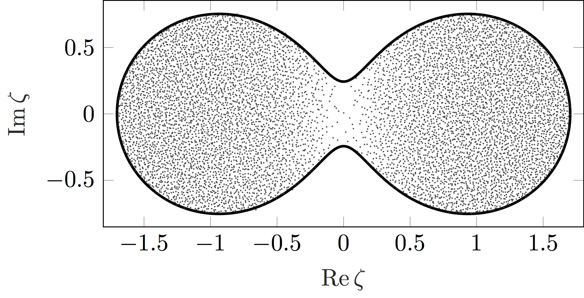
(a) $\{\zeta_{1},\zeta_{2}\}=\{\pm 0.97\}$

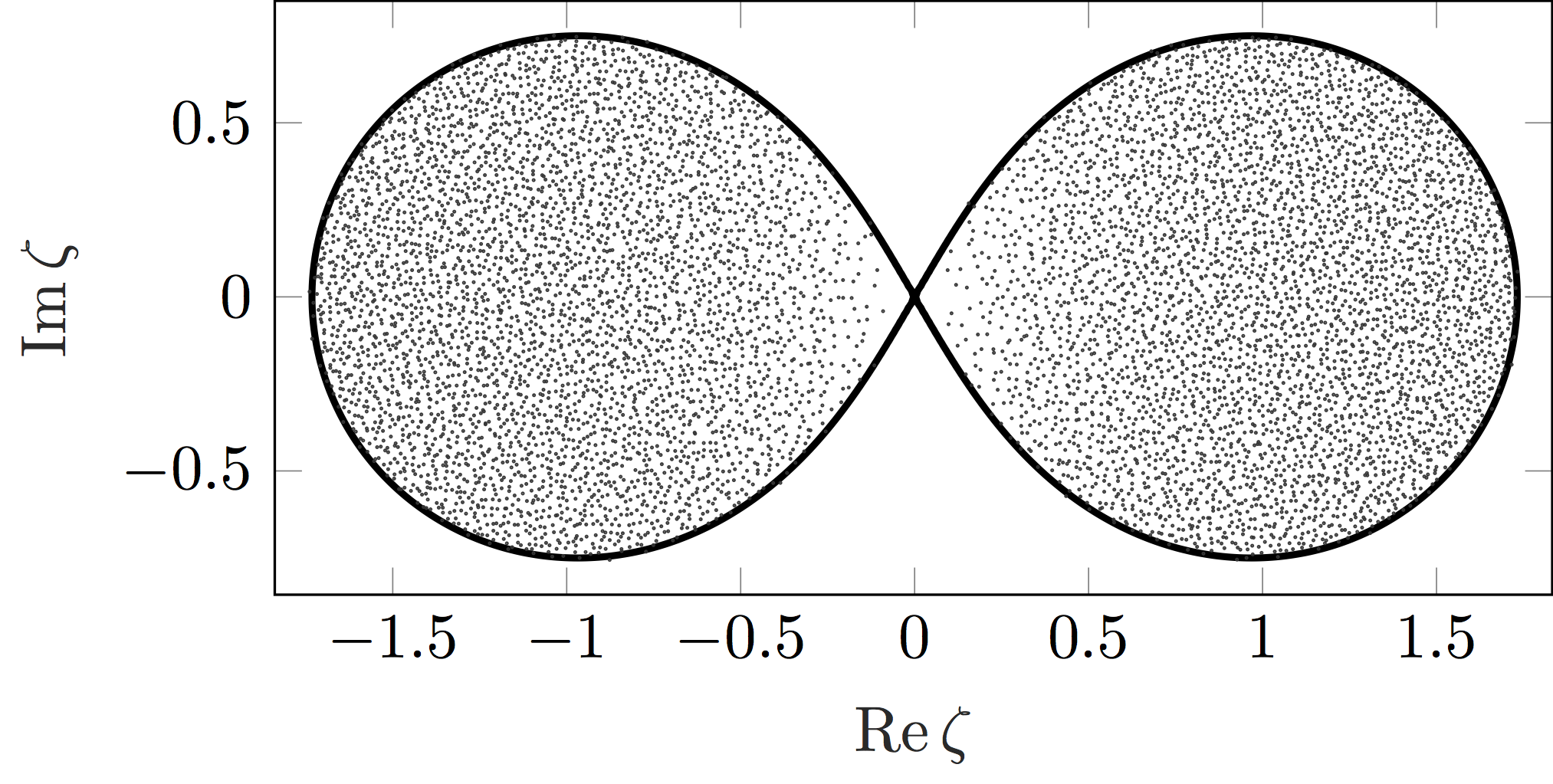
(b) $\{\zeta_{1},\zeta_{2}\}=\{\pm 1.0\}$

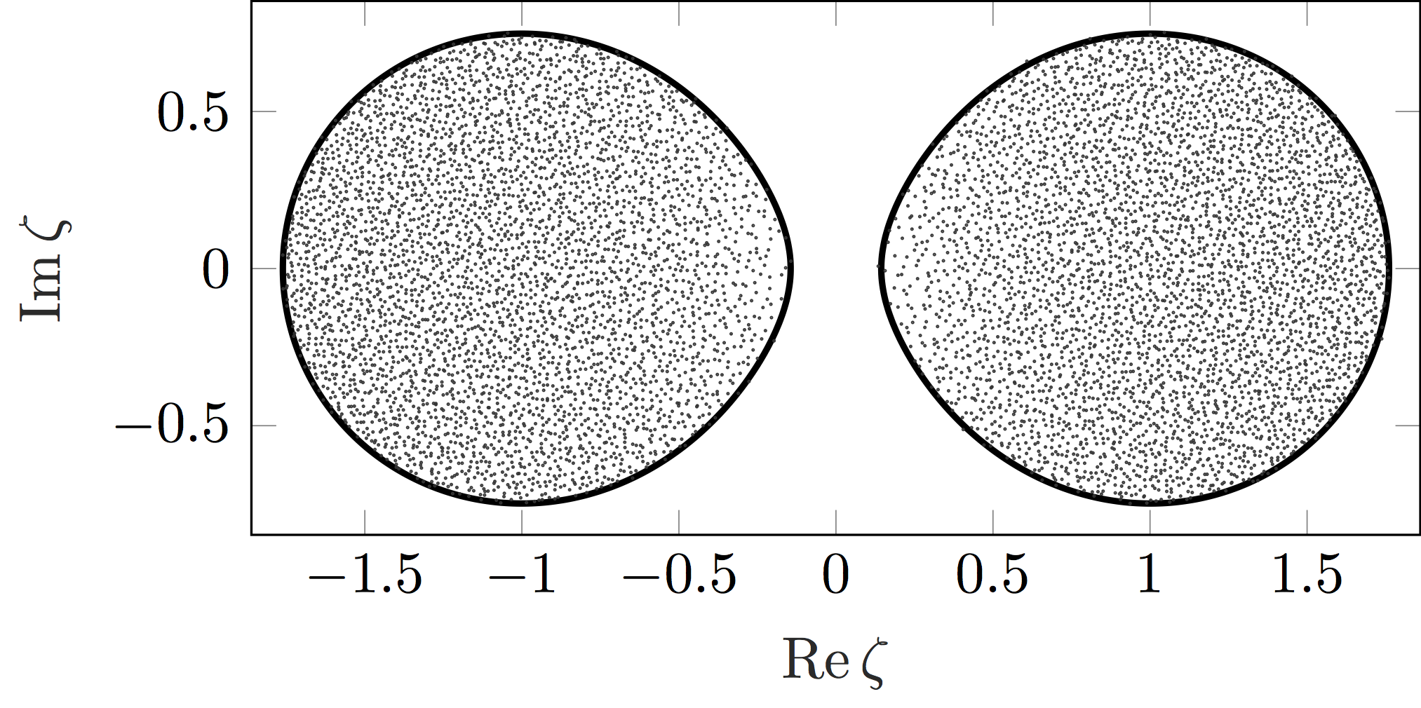
(c) $\{\zeta_{1},\zeta_{2}\}=\{\pm 1.03\}$

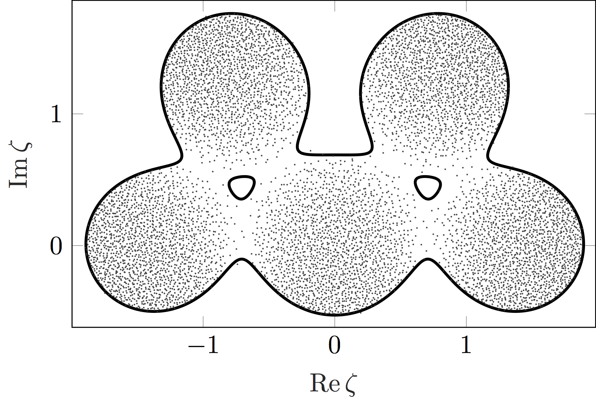
(d) $\{\zeta_{1},\ldots,\zeta_{5}\}=\{0,\pm 1.4,\pm 0.8+\mathrm{i}1.26\}$

Figure 1: Eigenvalues of sample random matrix with $N=8000$ and $\cap_{\varepsilon>0}{\mathbb{D}}_{\varepsilon}$.

The empirical density of states of a Hermitian matrix $\bm{H}\in\mathbb{C}^{L\times L}\otimes\mathbb{C}^{N\times N}$ is defined through

$$\mu_{\bm{H}}(\mathrm{d}\tau)\mathrel{\vbox{\hbox{\scriptsize.}\hbox{\scriptsize.}}}=\frac{1}{NL}\sum_{\lambda\in\operatorname{Spec}(\bm{H})}\delta_{\lambda}(\mathrm{d}\tau).$$ (2.16)

Theorem 2.7 (Global law for Hermitian Kronecker matrices).

Fix $L\in\mathbb{N}$. For $N\in\mathbb{N}$, let $\bm{H}_{N}\in\mathbb{C}^{L\times L}\otimes\mathbb{C}^{N\times N}$ be a Hermitian Kronecker random matrix as in (2.1) such that the bounds (2.9) – (2.12) are satisfied. Then there exists a sequence of deterministic probability measures $\rho_{N}$ on $\mathbb{R}$ such that the difference of $\rho_{N}$ and the empirical spectral measure $\mu_{\bm{H}_{N}}$, defined in (2.16), of $\bm{H}_{N}$ converges to zero weakly in probability, i.e.,

$$\lim_{N\to\infty}\int_{\mathbb{R}}f(\tau)(\mu_{\bm{H}_{N}}-\rho_{N})(\mathrm{d}\tau)=0$$ (2.17)

for all $f\in C_{0}(\mathbb{R})$ in probability. Here, $C_{0}(\mathbb{R})$ denotes the continuous functions on $\mathbb{R}$ vanishing at infinity.

Furthermore, there is a compact subset of $\mathbb{R}$ which contains the supports of all $\rho_{N}$. This compact set depends only on the model parameters.

Theorem 2.7 is proven in Appendix B. The measure $\rho_{N}$, the self-consistent density of states, can be obtained by solving the corresponding Dyson equation, see Definition 3.3 later. If the function $f$ is sufficiently regular then our proof combined with the Helffer-Sjöstrand formula yields an effective convergence rate of order $N^{-\delta}$ in (2.17).

3 Solution and stability of the Dyson equation

The general matrix Dyson equation (MDE) has been extensively studied in [3], but under conditions that exclude general Kronecker random matrices. Here, we relax these conditions and show how to extend some key results of [3] to our current setup. Our analysis of the MDE on the space of $n\times n$ matrices, ${{\mathcal{M}}}=\mathbb{C}^{n\times n}$, will then be applied to (2.6) with $n=2LN=KN$. On ${{\mathcal{M}}}=\mathbb{C}^{n\times n}$, we use the norms as defined in Subsection 1.1 and require the pair $(\bm{A},\bm{\mathcal{S}})$ to have the following properties:

Definition 3.1 (Data pair).

We call $(\bm{A},\bm{\mathcal{S}})$ a data pair if

• The imaginary part $\operatorname{Im}\bm{A}=\frac{1}{2\mathrm{i}}(\bm{A}-\bm{A}^{*})$ of the matrix $\bm{A}\in\mathbb{C}^{n\times n}$ is negative semidefinite.

• The linear operator $\bm{\mathcal{S}}:\mathbb{C}^{n\times n}\to\mathbb{C}^{n\times n}$ is self-adjoint with respect to the scalar product

  $$\langle{\bm{{R}}}\mspace{2.0mu},{\bm{{T}}}\rangle\,\mathrel{\vbox{\hbox{\scriptsize.}\hbox{\scriptsize.}}}=\,\frac{1}{n}\operatorname{Tr}[\bm{{R}}^{*}\bm{{T}}]\,,$$

  and preserves the cone of positive semidefinite matrices, i.e. it is positivity preserving.

For any data pair $(\bm{A},\bm{\mathcal{S}})$, the MDE then takes the form

$$-{\bm{M}}^{-1}(z)=z\mathds{1}-\bm{A}+\bm{\mathcal{S}}[{\bm{M}}(z)],\quad z\in\mathbb{H},$$ (3.1)

for a solution matrix ${\bm{M}}(z)\in\mathbb{C}^{n\times n}$. It was shown in this generality that the MDE, (3.1), has a unique solution under the constraint that the imaginary part $\mathrm{Im}\,{\bm{M}}(z)\mathrel{\vbox{\hbox{\scriptsize.}\hbox{\scriptsize.}}}=({\bm{M}}(z)-{\bm{M}}(z)^{*})/(2\mathrm{i})$ is positive definite [27]. We remark that $\mathrm{Im}\,\bm{A}$ being negative semidefinite is the most general condition for which our analysis is applicable. Furthermore, in [3], properties of the solution of (3.1) and the stability of (3.1) against small perturbations were studied in the general setup with Hermitian $\bm{{A}}$ and under the so-called flatness assumption,

$$\begin{split}\frac{c}{n}\operatorname{Tr}({\bm{R}})\leq\bm{\mathcal{S}}[{\bm{R}}]\leq\frac{C}{n}\operatorname{Tr}({\bm{R}})\,,\end{split}$$ (3.2)

for all positive definite ${\bm{R}}\in\mathbb{C}^{n\times n}$ with some constants $C>c>0$. Within Section 3 we will generalize certain results from [3] by dropping the flatness assumption (3.2) and the Hermiticity of $\bm{{A}}$. The results in this section, apart from (3.4b) below, follow by combining and modifying several arguments from [3]. We will only explain the main steps and refer to [3] for details. At the end of the section we translate these general results back to the setup of Kronecker matrices with the associated Dyson equation (2.6).

3.1 Solution of the Dyson equation

According to Proposition 2.1 in [3] the solution ${\bm{M}}$ to (3.1) has a Stieltjes transform representation

$$\begin{split}{\bm{M}}(z)\,=\,\int_{\mathbb{R}}\frac{\bm{{V}}(\mathrm{d}\tau)}{\tau-z}\,,\qquad z\in\mathbb{H}\,,\end{split}$$ (3.3)

where $\bm{{V}}$ is a compactly supported measure on $\mathbb{R}$ with values in positive semidefinite $n\times n$-matrices such that $\bm{{V}}(\mathbb{R})=\mathds{1}$, provided $\bm{A}$ is Hermitian. The following lemma strengthens the conclusion about the support properties for this measure compared to Proposition 2.1 in [3].

Lemma 3.2.

Let $(\bm{A},\bm{\mathcal{S}})$ be a data pair as in Definition 3.1 and ${\bm{M}}:\mathbb{H}\to\mathbb{C}^{n\times n}$ be the unique solution to (3.1) with positive definite imaginary part. Then

1. There is a unique measure $\bm{{V}}$ on $\mathbb{R}$ with values in positive semidefinite matrices and $\bm{{V}}(\mathbb{R})=\mathds{1}$ such that (3.3) holds true.

2. If $\bm{A}$ is Hermitian, then

   $$\operatorname{supp}\bm{{V}} \,\subset\,\operatorname{Spec}\bm{{A}}+[-2\lVert\bm{\mathcal{S}}\rVert^{1/2},2\lVert\bm{\mathcal{S}}\rVert^{1/2}],$$ (3.4a)

   $$\operatorname{Spec}\bm{{A}} \,\subset\,\operatorname{supp}\bm{{V}}+[-\lVert\bm{\mathcal{S}}\rVert^{1/2},\lVert\bm{\mathcal{S}}\rVert^{1/2}].$$ (3.4b)

Proof of Lemma 3.2.

The representation (3.3) follows exactly as in the proof of Proposition 2.1 in [3] even for $\bm{A}$ with negative semidefinite imaginary part. We now prove (3.4a) motivated by the same proof in [3]. For a matrix ${\bm{R}}\in\mathbb{C}^{n\times n}$, its smallest singular value is denoted by $\sigma_{\mathrm{min}}({\bm{R}})$. Note that $\sigma_{\mathrm{min}}(z-\bm{A})=\operatorname{dist}(z,\operatorname{Spec}\bm{A})$ since $\bm{A}$ is Hermitian. In the following, we fix $z\in\mathbb{H}$ such that $\operatorname{dist}(z,\operatorname{Spec}\bm{A})=\sigma_{\mathrm{min}}(z-\bm{A})>2\lVert\bm{\mathcal{S}}\rVert^{1/2}$.

Under the condition $\lVert{\bm{M}}(z)\rVert_{2}\leq\sigma_{\mathrm{min}}(z-\bm{A})/(2\lVert\bm{\mathcal{S}}\rVert)$, we obtain from (3.1)

$$\lVert{\bm{M}}(z)\rVert_{2}=\frac{1}{\sigma_{\mathrm{min}}(z-\bm{A}+\bm{\mathcal{S}}[{\bm{M}}(z)])}\leq\frac{1}{\sigma_{\mathrm{min}}(z-\bm{A})-\lVert\bm{\mathcal{S}}\rVert\lVert{\bm{M}}(z)\rVert_{2}}\leq\frac{2}{\operatorname{dist}(z,\operatorname{Spec}\bm{A})}.$$ (3.5)

Therefore, using $\sigma_{\mathrm{min}}(z-\bm{A})>2\lVert\bm{\mathcal{S}}\rVert^{1/2}$, we find a gap in the values $\lVert{\bm{M}}(z)\rVert_{2}$ can achieve

$$\lVert{\bm{M}}(z)\rVert_{2}\notin\Big{(}\frac{2}{\sigma_{\mathrm{min}}(z-\bm{A})},\frac{\sigma_{\mathrm{min}}(z-\bm{A})}{2\lVert\bm{\mathcal{S}}\rVert}\Big{)}.$$

For large values of $\eta=\mathrm{Im}\,z$, $\lVert{\bm{M}}(z)\rVert_{2}$ is smaller than the lower bound of this interval. Thus, since $\lVert{\bm{M}}(z)\rVert_{2}$ is a continuous function of $z$ and the set $\{w\in\mathbb{H}\colon\operatorname{dist}(w,\operatorname{Spec}\bm{A})>2\lVert\bm{\mathcal{S}}\rVert^{1/2}\}$ is path-connected, we conclude that (3.5) holds true for all $z\in\mathbb{H}$ satisfying $\operatorname{dist}(z,\operatorname{Spec}\bm{A})>2\lVert\bm{\mathcal{S}}\rVert^{1/2}$.

We take the imaginary part of (3.1) and use $\bm{A}=\bm{A}^{*}$ to obtain $\mathrm{Im}\,{\bm{M}}=\eta{\bm{M}}^{*}{\bm{M}}+{\bm{M}}^{*}\bm{\mathcal{S}}[\mathrm{Im}\,{\bm{M}}]{\bm{M}}.$ Solving this relation for $\mathrm{Im}\,{\bm{M}}$ and estimating its norm yields

$$\lVert\mathrm{Im}\,{\bm{M}}\rVert_{2}\leq\frac{\eta\lVert{\bm{M}}\rVert_{2}^{2}}{1-\lVert\bm{\mathcal{S}}\rVert\lVert{\bm{M}}\rVert_{2}^{2}}\leq\frac{4\eta}{\operatorname{dist}(z,\operatorname{Spec}\bm{A})^{2}-4\lVert\bm{\mathcal{S}}\rVert}.$$

Here, we employed $\lVert{\bm{M}}\rVert_{2}^{2}\lVert\bm{\mathcal{S}}\rVert<1$ by (3.5) and $\operatorname{dist}(z,\operatorname{Spec}\bm{A})>2\lVert\bm{\mathcal{S}}\rVert^{1/2}$. Hence, $\mathrm{Im}\,{\bm{M}}$ converges to zero locally uniformly on the set $\big{\{}z\in\mathbb{H}\colon\operatorname{dist}(z,\operatorname{Spec}\bm{A})>2\lVert\bm{\mathcal{S}}\rVert^{1/2}\big{\}}$ for $\eta\downarrow 0$. Therefore, $E\notin\operatorname{supp}\bm{{V}}$ if $\operatorname{dist}(E,\operatorname{Spec}\bm{A})>2\lVert\bm{\mathcal{S}}\rVert^{1/2}$. This concludes the proof of (3.4a).

We now prove (3.4b). From (3.1), we obtain

$$\bm{A}-z\mathds{1}={\bm{M}}^{-1}(\mathds{1}+{\bm{M}}\bm{\mathcal{S}}[{\bm{M}}])$$ (3.6)

for $z\in\mathbb{H}$. Since $\bm{{V}}(\mathbb{R})=1$, we have

$$\lVert{\bm{M}}\rVert_{2}\leq\frac{1}{\operatorname{dist}(z,\operatorname{supp}\bm{{V}})}.$$ (3.7)

Therefore, taking the inverse in (3.6) and applying (3.7) yield

$$\lVert(\bm{A}-z\mathds{1})^{-1}\rVert_{2}\leq\frac{1}{\operatorname{dist}(z,\operatorname{supp}\bm{{V}})(1-\lVert\bm{\mathcal{S}}\rVert\operatorname{dist}(z,\operatorname{supp}\bm{{V}})^{-2})}$$ (3.8)

for all $z\in\mathbb{H}$ satisfying $\operatorname{dist}(z,\operatorname{supp}\bm{{V}})^{2}>\lVert\bm{\mathcal{S}}\rVert$. Taking $\mathrm{Im}\,z\downarrow 0$ in (3.8), we see that the matrix $\bm{A}-E\mathds{1}$ is invertible for all $E\in\mathbb{R}$ satisfying $\operatorname{dist}(E,\operatorname{supp}\bm{{V}})^{2}>\lVert\bm{\mathcal{S}}\rVert$, showing (3.4b). ∎

In accordance with Definition 2.3 in [3] we define the self-consistent density of states as the unique measure whose Stieltjes transform is $n^{-1}\operatorname{Tr}{\bm{M}}$.

Definition 3.3 (Self-consistent density of states).

The measure

$$\rho(\mathrm{d}\tau)\mathrel{\vbox{\hbox{\scriptsize.}\hbox{\scriptsize.}}}=\frac{1}{n}\operatorname{Tr}\bm{V}(\mathrm{d}\tau)\,=\,\langle\bm{V}(\mathrm{d}\tau)\rangle$$ (3.9)

is called the self-consistent density of states. Clearly, ${\operatorname{supp}\rho}=\operatorname{supp}\bm{V}$. For the following lemma, we also define the harmonic extension of the self-consistent density of states $\rho\colon\mathbb{H}\to\mathbb{R}_{+}$ through

$$\rho(z)\mathrel{\vbox{\hbox{\scriptsize.}\hbox{\scriptsize.}}}=\frac{1}{\pi}\langle\mathrm{Im}\,{\bm{M}}(z)\rangle.$$ (3.10)

In the following we will use the short hand notation

$${d_{\rho}(z)}\mathrel{\vbox{\hbox{\scriptsize.}\hbox{\scriptsize.}}}=\operatorname{dist}(z,{\operatorname{supp}\rho})\,.$$

Lemma 3.4 (Bounds on ${\bm{M}}$ and ${\bm{M}}^{-1}$).

Let $(\bm{A},\bm{\mathcal{S}})$ be a data pair as in Definition 3.1.

1. For $z\in\mathbb{H}$, we have the bounds

   $$\lVert{\bm{M}}\rVert_{2}\leq \,\frac{1}{{d_{\rho}(z)}},$$ (3.11a)

   $$(\mathrm{Im}\,z)\lVert{\bm{M}}^{-1}\rVert_{2}^{-2}\mathds{1}\leq\mathrm{Im}\,{\bm{M}}\leq \,\frac{\mathrm{Im}\,z}{{d_{\rho}^{2}(z)}}\mathds{1},$$ (3.11b)

   $$\lVert{\bm{M}}^{-1}\rVert_{2}\leq \,\lvert z\rvert+\lVert\bm{A}\rVert_{2}+\lVert\bm{\mathcal{S}}\rVert\lVert{\bm{M}}\rVert_{2}.$$ (3.11c)

2. For $z\in\mathbb{H}$, we have the bound

   $$\rho(z)\leq\frac{\mathrm{Im}\,z}{\pi{d_{\rho}^{2}(z)}}.$$ (3.12)

Proof.

Using (3.3) immediately yields (3.11a) and the upper bound in (3.11b) since $\bm{{V}}(\mathbb{R})=\mathds{1}$. With $\eta=\mathrm{Im}\,z$ and taking the imaginary part of (3.1), we obtain

$$\mathrm{Im}\,{\bm{M}}=\eta{\bm{M}}^{*}{\bm{M}}-{\bm{M}}^{*}(\mathrm{Im}\,\bm{A}){\bm{M}}+{\bm{M}}^{*}\bm{\mathcal{S}}[\mathrm{Im}\,{\bm{M}}]{\bm{M}}\geq\eta{\bm{M}}^{*}{\bm{M}}$$

as $\mathrm{Im}\,\bm{A}\leq 0$, $\mathrm{Im}\,{\bm{M}}\geq 0$ and $\bm{\mathcal{S}}$ is positivity preserving. Since ${\bm{R}}^{*}{\bm{R}}\geq\lVert{\bm{R}}^{-1}\rVert_{2}^{-2}\mathds{1}$ for any ${\bm{R}}\in\mathbb{C}^{n\times n}$ the lower bound in (3.11b) follows. From (3.1), we obtain (3.11c). Since $\rho(z)=\pi^{-1}\langle\mathrm{Im}\,{\bm{M}}(z)\rangle$ the upper bound in (3.11b) implies (3.12). ∎

3.2 Stability of the Dyson equation

The goal of studying the stability of the Dyson equation in matrix form, (3.1), is to show that if some ${\bm{G}}$ satisfies

$$-\mathds{1}=(z\mathds{1}-\bm{A}+\bm{\mathcal{S}}[{\bm{G}}]){\bm{G}}+\bm{D}$$ (3.13)

for some small $\bm{D}$, then ${\bm{G}}$ is close to ${\bm{M}}$. It turns out that to a large extent this is a question about the invertibility of the stability operator $\bm{\mathcal{L}}\mathrel{\vbox{\hbox{\scriptsize.}\hbox{\scriptsize.}}}=\mathrm{Id}-{\bm{M}}\bm{\mathcal{S}}[{\,\cdot\,}]{\bm{M}}$ acting on $\mathbb{C}^{n\times n}$. From (3.1) and (3.13), we obtain the following equation

$$\bm{\mathcal{L}}[{\bm{G}}-{\bm{M}}]={\bm{M}}\bm{D}+{\bm{M}}\bm{\mathcal{S}}[{\bm{G}}-{\bm{M}}]({\bm{G}}-{\bm{M}})$$ (3.14)

relating the difference ${\bm{G}}-{\bm{M}}$ with $\bm{D}$. We will call (3.14) the stability equation. Under the assumption that ${\bm{G}}$ is not too far from ${\bm{M}}$, the question whether ${\bm{G}}-{\bm{M}}$ is comparable with $\bm{D}$ is determined by the invertibility of $\bm{\mathcal{L}}$ in (3.14) and the boundedness of the inverse.

In this subsection, we show that $\lVert\bm{\mathcal{L}}^{-1}\rVert$ is bounded, provided $\operatorname{dist}(z,\operatorname{supp}\bm{{V}})$ is bounded away from zero. In order to prove this bound on $\bm{\mathcal{L}}^{-1}$, we follow the symmetrization procedure for $\bm{\mathcal{L}}$ introduced in [3]. We introduce the operators ${\mathcal{C}}_{\bm{R}}\colon\mathbb{C}^{n\times n}\to\mathbb{C}^{n\times n}$ and ${\bm{\mathcal{F}}}\colon\mathbb{C}^{n\times n}\to\mathbb{C}^{n\times n}$ through

$${\mathcal{C}}_{\bm{R}}[\bm{Q}]={\bm{R}}\bm{Q}{\bm{R}},\qquad\qquad{\bm{\mathcal{F}}}\mathrel{\vbox{\hbox{\scriptsize.}\hbox{\scriptsize.}}}={\mathcal{C}}_{\bm{W}}{\mathcal{C}}_{\sqrt{\mathrm{Im}\,{\bm{M}}}}\bm{\mathcal{S}}{\mathcal{C}}_{\sqrt{\mathrm{Im}\,{\bm{M}}}}{\mathcal{C}}_{\bm{W}},$$

for $\bm{Q}\in\mathbb{C}^{n\times n}$. Furthermore, the matrix ${\bm{T}}\in\mathbb{C}^{n\times n}$, the unitary matrix ${\bm{U}}\in\mathbb{C}^{n\times n}$ and the positive definite matrix ${\bm{W}}\in\mathbb{C}^{n\times n}$ are defined through

$${\bm{T}}\mathrel{\vbox{\hbox{\scriptsize.}\hbox{\scriptsize.}}}={\mathcal{C}}_{\sqrt{\mathrm{Im}\,{\bm{M}}}}^{-1}[\mathrm{Re}\,{\bm{M}}]-\mathrm{i}\mathds{1},\qquad{\bm{U}}\mathrel{\vbox{\hbox{\scriptsize.}\hbox{\scriptsize.}}}=\frac{{\bm{T}}}{\lvert{\bm{T}}\rvert},\qquad{\bm{W}}\mathrel{\vbox{\hbox{\scriptsize.}\hbox{\scriptsize.}}}=\lvert{\bm{T}}\rvert^{1/2}.$$

With these notations, a direct calculation yields

$$\bm{\mathcal{L}}=\mathrm{Id}-{\mathcal{C}}_{\bm{M}}\bm{\mathcal{S}}={\mathcal{C}}_{\sqrt{\mathrm{Im}\,{\bm{M}}}}{\mathcal{C}}_{\bm{W}}{\mathcal{C}}_{{\bm{U}}^{*}}\big{(}{\mathcal{C}}_{\bm{U}}-{\bm{\mathcal{F}}}\big{)}{\mathcal{C}}_{\bm{W}}^{-1}{\mathcal{C}}_{\sqrt{\mathrm{Im}\,{\bm{M}}}}^{-1},$$ (3.15)

as in (4.39) of [3].

We remark that ${\mathcal{C}}_{\bm{R}}$ for ${\bm{R}}\in\mathbb{C}^{n\times n}$ is invertible if and only if ${\bm{R}}$ is invertible and ${\mathcal{C}}_{\bm{R}}^{-1}={\mathcal{C}}_{{\bm{R}}^{-1}}$ in this case. Similarly, ${\mathcal{C}}_{\bm{R}}^{*}={\mathcal{C}}_{{\bm{R}}^{*}}$.

Our goal is to verify $\lVert{\bm{\mathcal{F}}}\rVert_{\mathrm{sp}}\leq 1-c$ for some positive constant $c$ which yields $\lVert({\mathcal{C}}_{\bm{U}}-{\bm{\mathcal{F}}})^{-1}\rVert_{\mathrm{sp}}\leq c^{-1}$ as $\lVert{\mathcal{C}}_{\bm{U}}\rVert_{\mathrm{sp}}=1$. Then the boundedness of the other factors in (3.15) implies the bound on the inverse of the stability operator $\bm{\mathcal{L}}$.

Convention 3.5 (Comparison relation).

For nonnegative scalars or vectors $f$ and $g$, we will use the notation $f\lesssim g$ if there is a constant $c>0$, depending only on $\lVert\bm{\mathcal{S}}\rVert_{\mathrm{hs}\to\lVert{\,\cdot\,}\rVert}$ such that $f\leq cg$ and $f\sim g$ if $f\lesssim g$ and $f\gtrsim g$ both hold true. If the constant $c$ depends on an additional parameter (e.g. $\varepsilon>0$), then we will indicate this dependence by a subscript (e.g. $\lesssim_{\varepsilon}$).

Lemma 3.6.

Let $(\bm{A},\bm{\mathcal{S}})$ be a data pair as in Definition 3.1.

1. Uniformly for any $z\in\mathbb{H}$, we have

   $${d_{\rho}^{4}(z)}\lVert{\bm{M}}^{-1}\rVert_{2}^{-2}\mathds{1}\lesssim{\bm{W}}^{4}(\mathrm{Im}\,z)^{2}\lesssim\lVert{\bm{M}}\rVert_{2}^{2}\lVert{\bm{M}}^{-1}\rVert_{2}^{4}\mathds{1}.$$ (3.16)

2. There is a positive semidefinite $\bm{F}\in\mathbb{C}^{n\times n}$ such that $\lVert\bm{F}\rVert_{\mathrm{hs}}=1$ and ${\bm{\mathcal{F}}}[\bm{F}]=\lVert{\bm{\mathcal{F}}}\rVert_{\mathrm{sp}}\bm{F}$. Moreover,

   $$1-\lVert{\bm{\mathcal{F}}}\rVert_{\mathrm{sp}}=(\mathrm{Im}\,z)\frac{\langle{\bm{F}}\mspace{2.0mu},{{\mathcal{C}}_{{\bm{W}}}[\mathrm{Im}\,{\bm{M}}]}\rangle}{\langle{\bm{F}}\mspace{2.0mu},{{\bm{W}}^{-2}}\rangle}.$$ (3.17)

3. Uniformly for $z\in\mathbb{H}$, we have

   $$1-\lVert{\bm{\mathcal{F}}}\rVert_{\mathrm{sp}}\gtrsim{d_{\rho}^{4}(z)}\lVert{\bm{M}}^{-1}\rVert_{2}^{-4}.$$ (3.18)

The proof of this lemma is motivated by the proofs of Lemma 4.6 and Lemma 4.7 (i) in [3].

Proof.

We set $\eta\mathrel{\vbox{\hbox{\scriptsize.}\hbox{\scriptsize.}}}=\mathrm{Im}\,z$. We rewrite the definition of ${\bm{W}}$ and use the upper bound in (3.11b) to obtain

$${\bm{W}}^{4}={\mathcal{C}}^{-1}_{\sqrt{\mathrm{Im}\,{\bm{M}}}}({\mathcal{C}}_{\mathrm{Im}\,{\bm{M}}}+{\mathcal{C}}_{\mathrm{Re}\,{\bm{M}}})[(\mathrm{Im}\,{\bm{M}})^{-1}]\geq \,\eta^{-1}{d_{\rho}^{2}(z)}{\mathcal{C}}^{-1}_{\sqrt{\mathrm{Im}\,{\bm{M}}}}[{\bm{M}}{\bm{M}}^{*}+{\bm{M}}^{*}{\bm{M}}]$$

$$\gtrsim \,\lVert{\bm{M}}^{-1}\rVert_{2}^{-2}\eta^{-2}{d_{\rho}^{4}(z)}\mathds{1}.$$

Here, we also applied ${\bm{M}}{\bm{M}}^{*}+{\bm{M}}^{*}{\bm{M}}\geq 2\lVert{\bm{M}}^{-1}\rVert_{2}^{-2}\mathds{1}$ and the upper bound in (3.11b) again. This proves the lower bound in (3.16). Similarly, using ${\bm{M}}{\bm{M}}^{*}+{\bm{M}}^{*}{\bm{M}}\leq 2\lVert{\bm{M}}\rVert_{2}^{2}\mathds{1}$ and the lower bound in (3.11b) we obtain the upper bound in (3.16).

For the proof of (ii), we remark that ${\bm{\mathcal{F}}}$ preserves the cone of positive semidefinite matrices. Thus, by a version of the Perron-Frobenius theorem of cone preserving operators there is a positive semidefinite $\bm{F}$ such that $\lVert\bm{F}\rVert_{\mathrm{hs}}=1$ and ${\bm{\mathcal{F}}}\bm{F}=\lVert{\bm{\mathcal{F}}}\rVert_{\mathrm{sp}}\bm{F}$. Following the proof of (4.24) in [3] and noting that this proof uses neither the uniqueness of $\bm{F}$ nor its positive definiteness, we obtain (3.17).

The bound in (3.18) is obtained by plugging the lower bound in (3.16) and the lower bound in (3.11b) into (3.17). We start by estimating the numerator in (3.17). Using $\bm{F}\geq 0$, the cyclicity of the trace, (3.11b) and the lower bound in (3.16), we get

$$\langle{\bm{F}}\mspace{2.0mu},{{\mathcal{C}}_{\bm{W}}[\mathrm{Im}\,{\bm{M}}]}\rangle\geq\eta\big{\langle}\sqrt{\bm{F}}{\bm{W}}^{2}\sqrt{\bm{F}}\big{\rangle}\lVert{\bm{M}}^{-1}\rVert_{2}^{-2}\gtrsim\lVert{\bm{M}}^{-1}\rVert_{2}^{-3}{d_{\rho}^{2}(z)}\langle\bm{F}\rangle.$$ (3.19)

Similarly, we have

$$\langle{\bm{F}}\mspace{2.0mu},{{\bm{W}}^{-2}}\rangle=\big{\langle}\sqrt{\bm{F}}{\bm{W}}^{-2}\sqrt{\bm{F}}\big{\rangle}\lesssim\frac{\eta}{{d_{\rho}^{2}(z)}}\lVert{\bm{M}}^{-1}\rVert_{2}\langle\bm{F}\rangle.$$ (3.20)

Combining (3.19) and (3.20) in (3.17) yields (3.18) and concludes the proof of the lemma. ∎

Lemma 3.7 (Bounds on the inverse of the stability operator).

Let $(\bm{A},\bm{\mathcal{S}})$ be a data pair as in Definition 3.1.

1. The stability operator $\bm{\mathcal{L}}$ is invertible for all $z\in\mathbb{H}$. For fixed $E\in\mathbb{R}$ and uniformly for $\eta\geq\max\{1,\lvert E\rvert,\lVert\bm{A}\rVert_{2}\}$, we have

   $$\lVert\bm{\mathcal{L}}^{-1}(E+\mathrm{i}\eta)\rVert\lesssim 1.$$ (3.21)

2. Uniformly for $z\in\mathbb{H}$, we have

   $$\lVert\bm{\mathcal{L}}^{-1}(z)\rVert_{\mathrm{sp}}\lesssim\frac{\lVert{\bm{M}}(z)\rVert_{2}\lVert{\bm{M}}^{-1}(z)\rVert_{2}^{9}}{{d_{\rho}^{8}(z)}}.$$ (3.22)

3. Uniformly for $z\in\mathbb{H}$, we have

   $$\lVert\bm{\mathcal{L}}^{-1}(z)\rVert+\lVert(\bm{\mathcal{L}}^{-1}(z))^{*}\rVert\lesssim 1+\lVert{\bm{M}}(z)\rVert_{2}^{2}+\lVert{\bm{M}}(z)\rVert_{2}^{4}\lVert\bm{\mathcal{L}}^{-1}(z)\rVert_{\mathrm{sp}}.$$ (3.23)

Proof.

We start with the proof of (3.22). From the upper and lower bounds in (3.16) and (3.11b), respectively, we obtain

$$\lVert{\mathcal{C}}_{\bm{W}}\rVert\lesssim \,\frac{1}{\eta}\lVert{\bm{M}}\rVert_{2}\lVert{\bm{M}}^{-1}\rVert_{2}^{2}, \qquad\lVert{\mathcal{C}}_{\bm{W}}^{-1}\rVert\lesssim \,\frac{\eta}{{d_{\rho}^{2}(z)}}\lVert{\bm{M}}^{-1}\rVert_{2},$$ (3.24a)

$$\lVert{\mathcal{C}}_{\sqrt{\mathrm{Im}\,{\bm{M}}}}\rVert\lesssim \,\frac{\eta}{{d_{\rho}^{2}(z)}}, \qquad\lVert{\mathcal{C}}_{\sqrt{\mathrm{Im}\,{\bm{M}}}}^{-1}\rVert\lesssim \,\frac{1}{\eta}\lVert{\bm{M}}^{-1}\rVert_{2}^{2}.$$ (3.24b)

Since $\lVert{\mathcal{C}}_{\bm{T}}\rVert_{\mathrm{sp}}\leq\lVert{\mathcal{C}}_{\bm{T}}\rVert$ for Hermitian ${\bm{T}}\in\mathbb{C}^{n\times n}$ we conclude from (3.24), (3.18) and (3.11a)

$$\lVert\bm{\mathcal{L}}^{-1}\rVert_{\mathrm{sp}}\lesssim\frac{\lVert{\bm{M}}\rVert_{2}\lVert{\bm{M}}^{-1}\rVert_{2}^{5}}{{d_{\rho}^{4}(z)}}\lVert({\mathcal{C}}_{\bm{U}}-{\bm{\mathcal{F}}})^{-1}\rVert_{\mathrm{sp}}\lesssim\frac{\lVert{\bm{M}}\rVert_{2}\lVert{\bm{M}}^{-1}\rVert_{2}^{9}}{{d_{\rho}^{8}(z)}}.$$

For the proof of (3.23), we remark that $\lVert\bm{\mathcal{S}}\rVert_{\mathrm{hs}\to\lVert{\,\cdot\,}\rVert}\lesssim 1$ implies $\lVert\bm{\mathcal{S}}\rVert_{\lVert{\,\cdot\,}\rVert\to\mathrm{hs}}\lesssim 1$. Therefore, exactly as in the proof of (4.53) in [3], we obtain the first bound in (3.23). We similarly conclude the second bound from $\lVert(\bm{\mathcal{L}}^{-1})^{*}\rVert_{\mathrm{sp}}=\lVert\bm{\mathcal{L}}^{-1}\rVert_{\mathrm{sp}}$.

We conclude the proof of Lemma 3.7 by remarking that (3.21) is a consequence of (3.22), (3.11a), (3.23) and (3.11c). ∎

Corollary 3.8 (Lipschitz-continuity of ${\bm{M}}$).

If $(\bm{A},\bm{\mathcal{S}})$ is a data pair as in Definition 3.1 then there exists $c>0$ such that for each (possibly $N$-dependent) $\varepsilon\in(0,1]$ we have

$$\lVert{\bm{M}}(z_{1})-{\bm{M}}(z_{2})\rVert_{2}\lesssim(\varepsilon^{-c}+\lVert\bm{A}\rVert_{2}^{c})\lvert z_{1}-z_{2}\rvert$$ (3.25)

for all $z_{1},z_{2}\in\mathbb{H}$ such that $\mathrm{Im}\,z_{1},\mathrm{Im}\,z_{2}\geq\varepsilon$.

Proof.

We differentiate (3.1) with respect to $z$ and obtain $\bm{\mathcal{L}}[\partial_{z}{\bm{M}}]={\bm{M}}^{2}$. We invert $\bm{\mathcal{L}}$, use (3.22), (3.11a) and (3.11c) and follow the proof of (3.23). This yields (3.25) and hence concludes the proof of Corollary 3.8. ∎

3.3 Translation to results for Kronecker matrices

Here we translate the results of Subsections 3.1 and 3.2 into results about (2.6). In fact, we study (2.6) in a slightly more general setup. Motivated by the identification $\mathbb{C}^{2\times 2}\otimes\mathbb{C}^{L\times L}\cong\mathbb{C}^{2L\times 2L}$, we consider (2.6) on $\mathbb{C}^{K\times K}$ for some $K\in\mathbb{N}$ instead. The results of Subsections 3.1 and 3.2 are applied with $n=KN$. Moreover, the special $a_{j}^{\zeta}$ defined in (2.5) are replaced by general $a_{j}\in\mathbb{C}^{K\times K}$. Therefore, the parameter $\zeta$ will not be present throughout this subsection. We thus look at the Dyson equation in vector form

$$-\frac{1}{m_{j}(z)}=z\mathds{1}-a_{j}+{\mathscr{S}}_{j}[\bm{m}(z)],$$ (3.26)

where $z\in\mathbb{H}$, $m_{j}(z)\in\mathbb{C}^{K\times K}$ for $j\in[N]$, $\bm{m}(z)\mathrel{\vbox{\hbox{\scriptsize.}\hbox{\scriptsize.}}}=(m_{1}(z),\ldots m_{N}(z))$ and ${\mathscr{S}}_{j}$ is defined as in (2.4).

Recall that the definition of ${\mathscr{S}}_{j}$ involves coefficients $s_{ij}^{\mu}$ and $t_{ij}^{\nu}$ as well as matrices $\alpha_{\mu}$ and $\beta_{\nu}$. Next, we formulate assumptions on ${\mathscr{S}}$ in terms of these data as well as assumptions on $a_{1},\ldots,a_{N}$.

Assumptions 3.9.

1. For all $\mu,\nu\in[\ell]$ and $i,j\in[N]$, we have nonnegative scalars $s_{ij}^{\mu}\in\mathbb{R}$ and $t_{ij}^{\nu}\in\mathbb{R}$ satisfying (2.9). Furthermore, $s_{ij}^{\mu}=s_{ji}^{\mu}$ for all $i,j\in[N]$ and $\mu\in[\ell]$.

2. For $\mu,\nu\in[\ell]$, we have $\alpha_{\mu},\beta_{\nu}\in\mathbb{C}^{K\times K}$ and $\alpha_{\mu}$ is Hermitian. There is $\alpha^{*}>0$ such that

   $$\max_{\mu\in[\ell]}\lvert\alpha_{\mu}\rvert\leq\alpha^{*},\qquad\max_{\nu\in[\ell]}\lvert\beta_{\nu}\rvert\leq\alpha^{*}.$$ (3.27)

3. The matrices $a_{1},\ldots,a_{N}\in\mathbb{C}^{K\times K}$ have a negative semidefinite imaginary part, $\mathrm{Im}\,a_{j}\leq 0$.

The conditions in (i) of Assumptions 3.9 are motivated by the definition of the variances in (2.3). In particular, since $X_{\mu}$ is Hermitian the variances from (2.3) satisfy $s_{ij}^{\mu}=s_{ji}^{\mu}$.

In order to apply the results of Subsections 3.1 and 3.2 to (3.26), we now relate it to the matrix Dyson equation (MDE) (3.1). It turns out that (3.26) is a special case when the MDE on ${{\mathcal{M}}}=\mathbb{C}^{K\times K}\otimes\mathbb{C}^{N\times N}$ is restricted to the block diagonal matrices

$${{\mathcal{D}}}\mathrel{\vbox{\hbox{\scriptsize.}\hbox{\scriptsize.}}}=\operatorname{span}\{a\otimes D\colon a\in\mathbb{C}^{K\times K},D\in\mathbb{C}^{N\times N}\text{ diagonal}\}\subset{{\mathcal{M}}}.$$ (3.28)

We recall $E_{ll}$, ${\mathscr{S}}_{l}$ and $P_{ll}$ from (1.6), (2.4) and (1.7), respectively, and define $\bm{A}\in{{\mathcal{M}}}$ and $\bm{\mathcal{S}}\colon{{\mathcal{M}}}\to{{\mathcal{M}}}$ through

$$\bm{A}\mathrel{\vbox{\hbox{\scriptsize.}\hbox{\scriptsize.}}}=\sum_{l=1}^{N}a_{l}\otimes E_{ll},\qquad\bm{\mathcal{S}}[{\bm{R}}]\mathrel{\vbox{\hbox{\scriptsize.}\hbox{\scriptsize.}}}=\sum_{l=1}^{N}{\mathscr{S}}_{l}[(P_{11}{\bm{R}},\ldots,P_{NN}{\bm{R}})]\otimes E_{ll}.$$ (3.29)

With these definitions, the Dyson equation in vector form, (3.26), can be rewritten in the matrix form (3.1) for a solution matrix ${\bm{M}}\in{{\mathcal{M}}}$. In the following, we will refer to (3.1) with these choices of ${{\mathcal{M}}}$, $\bm{A}$ and $\bm{\mathcal{S}}$ as the Dyson equation in matrix form.

In the remainder of the paper, we will consider the Dyson equation in matrix form, (3.1), exclusively with the choices of $\bm{A}$ and $\bm{\mathcal{S}}$ from (3.29). We have the following connection between (3.26) and (3.1). If ${\bm{M}}$ is a solution of (3.1) then, since the range of $\bm{\mathcal{S}}$ is contained in ${{\mathcal{D}}}$ and $\bm{A}\in{{\mathcal{D}}}$, we have ${\bm{M}}\in{{\mathcal{D}}}$, i.e, it can be written as

$${\bm{M}}(z)=\sum_{j=1}^{N}m_{j}(z)\otimes E_{jj}$$ (3.30)

for some unique $m_{1}(z),\ldots,m_{N}(z)\in\mathbb{C}^{K\times K}$. Moreover, these $m_{i}$ solve (3.26). Conversely, if $\bm{m}=(m_{1},\ldots,m_{N})\in(\mathbb{C}^{K\times K})^{N}$ solves (3.26) then ${\bm{M}}$ defined via (3.30) is a solution of (3.1). Furthermore, if ${\bm{M}}$ satisfies (3.30) then $\mathrm{Im}\,{\bm{M}}$ is positive definite if and only if $\mathrm{Im}\,m_{j}$ is positive definite for all $j\in[N]$. This correspondence yields the following translation of Lemma 3.2 to the setting for Kronecker random matrices, Proposition 3.10 below.

For part (ii), we recall $\lVert\bm{r}\rVert=\max_{i=1}^{N}\lvert r_{i}\rvert$ for $\bm{r}=(r_{1},\ldots,r_{N})\in(\mathbb{C}^{K\times K})^{N}$ and that $\lVert{\mathscr{S}}\rVert$ denotes the operator norm of ${\mathscr{S}}\colon(\mathbb{C}^{K\times K})^{N}\to(\mathbb{C}^{K\times K})^{N}$ induced by $\lVert{\,\cdot\,}\rVert$. We also used that $\lVert{\mathscr{S}}\rVert=\lVert\bm{\mathcal{S}}\rVert$, which is easy to see since ${\mathscr{S}}=\bm{\mathcal{S}}$ on the block diagonal matrices $(\mathbb{C}^{K\times K})^{N}\cong{{\mathcal{D}}}$ and $\bm{\mathcal{S}}=0$ on the orthogonal complement ${{\mathcal{D}}}^{\perp}$. The orthogonal complement is defined with respect to the scalar product on ${{\mathcal{M}}}$ introduced in (1.5). Furthermore, we remark that the identity (3.30) implies

$$\lVert{\bm{M}}\rVert_{2}=\lVert\bm{m}\rVert.$$

Proposition 3.10 (Existence, uniqueness of $\bm{m}$).

Under Assumptions 3.9 we have

1. There is a unique function $\bm{m}\colon\mathbb{H}\to(\mathbb{C}^{K\times K})^{N}$ such that the components $\bm{m}(z)=(m_{1}(z),\ldots,m_{N}(z))$ satisfy (3.26) for $z\in\mathbb{H}$ and all $j\in[N]$ and $\mathrm{Im}\,m_{j}(z)$ is positive definite for all $z\in\mathbb{H}$ and all $j\in[N]$. Furthermore, for each $j\in[N]$, there is a measure $v_{j}$ on $\mathbb{R}$ with values in the positive semidefinite matrices of $\mathbb{C}^{K\times K}$ such that $v_{j}(\mathbb{R})=\mathds{1}$ and for all $z\in\mathbb{H}$, we have

   $$m_{j}(z)=\int_{\mathbb{R}}\frac{v_{j}(\mathrm{d}\tau)}{\tau-z}.$$ (3.31)

2. If $a_{j}$ is Hermitian, i.e., $a_{j}=a_{j}^{*}$ for all $j\in[N]$ then the union of the supports of $v_{j}$ is comparable with the union of the spectra of the $a_{j}$ in the following sense

   $$\bigcup_{j=1}^{N}\operatorname{supp}v_{j} \,\subset\,\bigcup_{j=1}^{N}\operatorname{Spec}a_{j}+[-2\lVert{\mathscr{S}}\rVert^{1/2},2\lVert{\mathscr{S}}\rVert^{1/2}],$$ (3.32a)

   $$\bigcup_{j=1}^{N}\operatorname{Spec}a_{j} \,\subset\,\bigcup_{j=1}^{N}\operatorname{supp}v_{j}+[-\lVert{\mathscr{S}}\rVert^{1/2},\lVert{\mathscr{S}}\rVert^{1/2}].$$ (3.32b)

Proof of Lemma 2.2.

Using the identification $\mathbb{C}^{2\times 2}\otimes\mathbb{C}^{L\times L}\cong\mathbb{C}^{K\times K}$ for $K=2L$ and the definitions in (2.2) and (2.5), the lemma is an immediate consequence of Proposition 3.10 with $a_{j}=a_{j}^{\zeta}$ for $j\in[N]$ since the proof of the proposition only uses the qualitative conditions in Assumptions 3.9. ∎

Proposition 3.10 asserts that there is a measure $V_{\bm{M}}$ on $\mathbb{R}$ with values in the positive semidefinite elements of ${{\mathcal{D}}}\subset{{\mathcal{M}}}$ such that for $z\in\mathbb{H}$, we have

$$V_{\bm{M}}(\mathrm{d}\tau)\mathrel{\vbox{\hbox{\scriptsize.}\hbox{\scriptsize.}}}=\sum_{j=1}^{N}v_{j}(\mathrm{d}\tau)\otimes E_{jj},\qquad{\bm{M}}(z)=\int_{\mathbb{R}}\frac{1}{\tau-z}V_{\bm{M}}(\mathrm{d}\tau).$$ (3.33)

Clearly, we have $V_{\bm{M}}=\bm{V}$ for the unique measure $\bm{V}$ with values in positive semidefinite matrices that satisfies (3.3). And we have $\operatorname{supp}V_{\bm{M}}={\operatorname{supp}\rho}$ with the self-consistent density of states defined in (3.9). Note that in this setup

$$\rho(\mathrm{d}\tau)=\frac{1}{NK}\sum_{j=1}^{N}\operatorname{Tr}v_{j}(\mathrm{d}\tau)\,,$$ (3.34)

with the $\mathbb{C}^{K\times K}$-matrix valued measures $v_{j}$ defined through (3.31).

In the remainder of the paper, $\bm{m}=(m_{1},\ldots,m_{N})$ and ${\bm{M}}$ always denote the unique solutions of (3.26) and (3.1), respectively, connected via (3.30). We now modify the concept of comparison relation introduced in Convection 3.5 so that inequalities are understood up to constants depending only on the model parameters from Assumption 3.9.

Convention 3.11 (Comparison relation).

From here on we use the comparison relation introduced in Convection 3.5 so that the constants implicitly hidden in this notation may depend only on $K$, $\ell$, $\kappa_{1}$ from (2.9) and $\alpha^{*}$ from (3.27).

Lemma 3.12 (Bounds on ${\mathscr{S}}$).

Assumptions 3.9 imply

$$\lVert{\mathscr{S}}\rVert_{\mathrm{sp}}\,\lesssim\,1,\qquad\lVert{\mathscr{S}}\rVert\,\lesssim\,1.$$ (3.35)

Proof.

Direct estimates of ${\mathscr{S}}[\bm{a}]$ for $\bm{a}\in(\mathbb{C}^{K\times K})^{N}$ starting from the definition of ${\mathscr{S}}_{i}$, (2.4), and using the assumptions (2.9) and (3.27) yield the bounds in (3.35). ∎

Similarly to $\bm{\mathcal{L}}$, we now introduce the stability operator of the Dyson equation in vector form, (3.26). In fact, it is defined through

$${\mathscr{L}}\colon(\mathbb{C}^{K\times K})^{N}\to(\mathbb{C}^{K\times K})^{N},\quad{\mathscr{L}}(r_{1},\ldots,r_{N})\mathrel{\vbox{\hbox{\scriptsize.}\hbox{\scriptsize.}}}=(r_{i}-m_{i}{\mathscr{S}}_{i}[\bm{r}]m_{i})_{i=1}^{N}.$$ (3.36)

We remark that $\bm{\mathcal{S}}$ and thus $\bm{\mathcal{L}}$ leave the set of block diagonal matrices ${{\mathcal{D}}}$ defined in (3.28) invariant. The operators ${\mathscr{S}}$ and ${\mathscr{L}}$ are the restrictions of $\bm{\mathcal{S}}$ and $\bm{\mathcal{L}}$ to ${{\mathcal{D}}}$. In particular, we have

$$\lVert{\mathscr{L}}^{-1}\rVert_{\mathrm{sp}}\leq\lVert\bm{\mathcal{L}}^{-1}\rVert_{\mathrm{sp}},\qquad\lVert\bm{\mathcal{L}}^{-1}\rVert_{\mathrm{sp}}\leq\max\{1,\lVert{\mathscr{L}}^{-1}\rVert_{\mathrm{sp}}\},\qquad\lVert{\mathscr{L}}^{-1}\rVert\leq\lVert\bm{\mathcal{L}}^{-1}\rVert,$$ (3.37)

since $\bm{\mathcal{L}}$ acts as the identity map on the orthogonal complement ${{\mathcal{D}}}^{\perp}$ of the block diagonal matrices. Here, the orthogonal complement is defined with respect to the scalar product on ${{\mathcal{M}}}$ introduced in (1.5). Moreover, ${\mathscr{L}}$ is invertible if and only if $\bm{\mathcal{L}}$ is invertible. Using (3.37) the bounds on $\bm{\mathcal{L}}$ from Lemma 3.7 can be translated into bounds on ${\mathscr{L}}$

4 Hermitian Kronecker matrices

The analysis of a non-Hermitian random matrix usually starts with Girko’s Hermitization procedure. It provides a technique to extract spectral information about a non-Hermitian matrix ${\bm{X}}$ from a family of Hermitian matrices $(\bm{H}^{\zeta})_{\zeta\in\mathbb{C}}$ defined through

$$\bm{H}^{\zeta}\mathrel{\vbox{\hbox{\scriptsize.}\hbox{\scriptsize.}}}=\begin{pmatrix}0&1\\ 0&0\end{pmatrix}\otimes{\bm{X}}+\begin{pmatrix}0&0\\ 1&0\end{pmatrix}\otimes{\bm{X}}^{*}-\begin{pmatrix}0&\zeta\\ \bar{\zeta}&0\end{pmatrix}\otimes\mathds{1},\qquad\zeta\in\mathbb{C}.$$ (4.1)

Applying Girko’s Hermitization procedure to a Kronecker random matrix ${\bm{X}}$ as in (2.1) generates a Hermitian Kronecker matrix $\bm{H}^{\zeta}\in\mathbb{C}^{2\times 2}\otimes\mathbb{C}^{L\times L}\otimes\mathbb{C}^{N\times N}$. However, similarly to our analysis in Section 3, we study more general Kronecker matrices $\bm{H}\in\mathbb{C}^{K\times K}\otimes\mathbb{C}^{N\times N}$ as in (4.2) below for $K,N\in\mathbb{N}$. This is motivated by the identification $\mathbb{C}^{2\times 2}\otimes\mathbb{C}^{L\times L}\cong\mathbb{C}^{2L\times 2L}$.

For $K,N\in\mathbb{N}$, let the random matrix $\bm{H}\in\mathbb{C}^{K\times K}\otimes\mathbb{C}^{N\times N}$ be defined through

$$\bm{H}\mathrel{\vbox{\hbox{\scriptsize.}\hbox{\scriptsize.}}}=\sum_{\mu=1}^{\ell}\alpha_{\mu}\otimes X_{\mu}+\sum_{\nu=1}^{\ell}\left(\beta_{\nu}\otimes Y_{\nu}+\beta_{\nu}^{*}\otimes Y_{\nu}^{*}\right)+\sum_{i=1}^{N}a_{i}\otimes E_{ii}.$$ (4.2)

Furthermore, we make the following assumptions. Let $\ell\in\mathbb{N}$. For $\mu\in[\ell]$, let ${\alpha}_{\mu}\in\mathbb{C}^{K\times K}$ be a deterministic Hermitian matrix and $X_{\mu}=X_{\mu}^{*}\in\mathbb{C}^{N\times N}$ a Hermitian random matrix with centered and independent entries (up to the Hermitian symmetry constraint). For $\nu\in[\ell]$, let ${\beta}_{\nu}\in\mathbb{C}^{K\times K}$ be a deterministic matrix and $Y_{\nu}$ a random matrix with centered and independent entries. We also assume that $X_{1},\ldots,X_{\ell},Y_{1},\ldots,Y_{\ell}$ are independent. Let $a_{1},\ldots,a_{N}\in\mathbb{C}^{K\times K}$ be some deterministic matrices with negative semidefinite imaginary part. We recall that $E_{ii}$ was defined in (1.6) and introduce the expectation $\bm{A}\mathrel{\vbox{\hbox{\scriptsize.}\hbox{\scriptsize.}}}=\mathbb{E}\bm{H}=\sum_{i=1}^{N}a_{i}\otimes E_{ii}$.

If $\bm{A}$ is a Hermitian matrix then $\bm{H}$ as in (4.2) with the above properties is a Hermitian Kronecker random matrix in the sense of Definition 2.1. As in the setup from (2.1), the matrices $\alpha_{1},\ldots\alpha_{\ell},\beta_{1},\ldots,{\beta}_{\ell}$ are called structure matrices.

Since the imaginary parts of $a_{1},\ldots,a_{N}$ are negative semidefinite, the same holds true for the imaginary part of $\bm{A}$ and $\bm{H}$. Hence, the matrix $\bm{H}-z\mathds{1}$ is invertible for all $z\in\mathbb{H}$. For $z\in\mathbb{H}$, we therefore introduce the resolvent ${\bm{G}}(z)$ of $\bm{H}$ and its “matrix elements” $G_{ij}(z)\mathrel{\vbox{\hbox{\scriptsize.}\hbox{\scriptsize.}}}=P_{ij}{\bm{G}}\in\mathbb{C}^{K\times K}$ for $i,j\in[N]$ defined through

$${\bm{G}}(z)\mathrel{\vbox{\hbox{\scriptsize.}\hbox{\scriptsize.}}}=(\bm{H}-z\mathds{1})^{-1},\qquad\qquad{\bm{G}}(z)=\sum_{i,j=1}^{N}G_{ij}(z)\otimes E_{ij}.$$

We recall that $P_{ij}$ has been defined in (1.7). Our goal is to show that $G_{ij}$ is small for $i\neq j$ and $G_{ii}$ is well approximated by the deterministic matrix $m_{i}(z)\in\mathbb{C}^{K\times K}$ in the regime where $K\in\mathbb{N}$ is fixed and $N\in\mathbb{N}$ is large.

Apart from the above listed qualitative assumptions, we will need the following quantitative assumptions. To formulate them we use the same notation as before, i.e., the entries of $X_{\mu}$ and $Y_{\nu}$ are denoted by $X_{\mu}=(x_{ij}^{\mu})_{i,j=1}^{N}$ and $Y_{\nu}=(y_{ij}^{\nu})_{i,j=1}^{N}$ and their variances by $s_{ij}^{\mu}\mathrel{\vbox{\hbox{\scriptsize.}\hbox{\scriptsize.}}}=\mathbb{E}\lvert x_{ij}^{\mu}\rvert^{2}$ and $t_{ij}^{\nu}\mathrel{\vbox{\hbox{\scriptsize.}\hbox{\scriptsize.}}}=\mathbb{E}\lvert y_{ij}^{\nu}\rvert^{2}$ (cf. (2.3)).

Assumptions 4.1.

We assume that all variances $s_{ij}^{\mu}$ and $t_{ij}^{\mu}$ satisfy (2.9) and the entries $x_{ij}^{\mu}$ and $y_{ij}^{\nu}$ of the random matrices fulfill the moment bounds (2.10). Furthermore, the structure matrices satisfy (3.27).

In this section, the model parameters are defined to be $K$, $\ell$, $\kappa_{1}$ from (2.9), the sequence $(\varphi_{p})_{p\in\mathbb{N}}$ from (2.10) and $\alpha^{*}$ from (3.27), so the relation $\lesssim$ indicates an inequality up to a multiplicative constant depending on these model parameters. Moreover, for the real and imaginary part of the spectral parameter $z$ we will write $E=\mathrm{Re}\,z$ and $\eta=\mathrm{Im}\,z$, respectively.

4.1 Error term in the perturbed Dyson equation

We introduce the notion of stochastic domination, a high probability bound up to $N^{\varepsilon}$ factors.

Definition 4.2 (Stochastic domination).

If $\Phi=(\Phi^{(N)})_{N}$ and $\Psi=(\Psi^{(N)})_{N}$ are two sequences of nonnegative random variables, then we say that $\Phi$ is stochastically dominated by $\Psi$, $\Phi\prec\Psi$, if for all $\varepsilon>0$ and $D>0$ there is a constant $C(\varepsilon,D)$ such that

$$\mathbb{P}\left(\Phi^{(N)}\geq N^{\varepsilon}\Psi^{(N)}\right)\leq\frac{C(\varepsilon,D)}{N^{D}}$$ (4.3)

for all $N\in\mathbb{N}$ and the function $(\varepsilon,D)\mapsto C(\varepsilon,D)$ depends only on the model parameters. If $\Phi$ or $\Psi$ depend on some additional parameter $\delta$ and the function $(\varepsilon,D)\mapsto C(\varepsilon,D)$ additionally depends on $\delta$ then we write $\Phi\prec_{\delta}\Psi$.

We set $h_{ij}\mathrel{\vbox{\hbox{\scriptsize.}\hbox{\scriptsize.}}}=P_{ij}\bm{H}\in\mathbb{C}^{K\times K}$. Using $P_{lm}\bm{A}=a_{l}\delta_{lm}$, $\mathbb{E}\,x_{ik}^{\mu}=0$, $\mathbb{E}\,y_{ik}^{\nu}=0$, (2.9), (3.27) and (2.10) we trivially obtain

$$\lvert P_{ik}\left(\bm{H}-\bm{A}\right)\rvert=\lvert h_{ik}-a_{i}\delta_{ik}\rvert\prec N^{-1/2}.$$ (4.4)

For $B\subset[N]$ we set

$$\bm{H}^{B}\mathrel{\vbox{\hbox{\scriptsize.}\hbox{\scriptsize.}}}=\sum_{i,j=1}^{N}h_{ij}^{B}\otimes E_{ij},\qquad h_{ij}^{B}\mathrel{\vbox{\hbox{\scriptsize.}\hbox{\scriptsize.}}}=h_{ij}\chi(i,j\notin B),$$

and denote the resolvent of $\bm{H}^{B}$ by ${\bm{G}}^{B}(z)\mathrel{\vbox{\hbox{\scriptsize.}\hbox{\scriptsize.}}}=\left(\bm{H}^{B}-z\mathds{1}\right)^{-1}$ for $z\in\mathbb{H}$. Since $\mathrm{Im}\,\bm{H}^{B}=\mathrm{Im}\,\bm{A}^{B}\leq 0$ for $B\subset[N]$, the matrix $(\bm{H}^{B}-z\mathds{1})$ is invertible for all $z\in\mathbb{H}$ and

$$\lVert{\bm{G}}^{B}(z)\rVert_{2}\leq\frac{1}{\mathrm{Im}\,z}.$$ (4.5)

In the following, we will use the convention

$$\sum_{k\in A}^{B}\mathrel{\vbox{\hbox{\scriptsize.}\hbox{\scriptsize.}}}=\sum_{k\in A\setminus B}$$

for $A,B\subset[N]$ and $B\subset A$. If $A=[N]$ then we simply write $\sum_{k}^{B}$.

For $i\in[N]$, starting from the Schur complement formula,

$$-\frac{1}{G_{ii}}=z-h_{ii}+\sum_{k,l}^{\{i\}}h_{ik}G_{kl}^{\{i\}}h_{li},$$ (4.6)

and using the definition of ${\mathscr{S}}_{i}$ in (2.4), we obtain the perturbed Dyson equation

$$-\frac{1}{g_{i}}\,=\,z-a_{i}+{\mathscr{S}}_{i}[\bm{g}]+d_{i}.$$ (4.7)

Here, we introduced

$$g_{i}\mathrel{\vbox{\hbox{\scriptsize.}\hbox{\scriptsize.}}}=G_{ii},\qquad\bm{g}\mathrel{\vbox{\hbox{\scriptsize.}\hbox{\scriptsize.}}}=(g_{1},\ldots,g_{N})\in(\mathbb{C}^{K\times K})^{N}$$ (4.8)

and the error term $d_{i}\in\mathbb{C}^{K\times K}$. We remark that (4.7) is a perturbed version of the Dyson equation in vector form, (3.26), and recall that $\bm{m}$ denotes its unique solution (cf. Proposition 3.10). To represent the error term $d_{i}$ in (4.7), we use $h_{ik}=a_{i}\delta_{ik}+\sum_{\mu}x_{ik}^{\mu}\alpha_{\mu}+\sum_{\nu}\left(y_{ik}^{\nu}\beta_{\nu}+\overline{y_{ki}^{\nu}}\beta_{\nu}^{*}\right)$ and write $d_{i}\mathrel{\vbox{\hbox{\scriptsize.}\hbox{\scriptsize.}}}=d_{i}^{(1)}+\ldots+d_{i}^{(8)}$, where

$$d^{(1)}_{i} \mathrel{\vbox{\hbox{\scriptsize.}\hbox{\scriptsize.}}}=\,-h_{ii}+a_{i},$$ (4.9a)

$$d^{(2)}_{i} \mathrel{\vbox{\hbox{\scriptsize.}\hbox{\scriptsize.}}}=\,\sum_{k}^{\{i\}}\Big{(}\sum_{\mu}\alpha_{\mu}G_{kk}^{\{i\}}\alpha_{\mu}\left(\lvert x_{ik}^{\mu}\rvert^{2}-s_{ik}^{\mu}\right)+\sum_{\nu}\left((\lvert y_{ik}^{\nu}\rvert^{2}-t_{ik}^{\nu})\beta_{\nu}G_{kk}^{\{i\}}\beta_{\nu}^{*}+(\lvert y_{ki}^{\nu}\rvert^{2}-t_{ki}^{\nu})\beta_{\nu}^{*}G_{kk}^{\{i\}}\beta_{\nu}\right)\Big{)},$$ (4.9b)

$$d^{(3)}_{i} \mathrel{\vbox{\hbox{\scriptsize.}\hbox{\scriptsize.}}}=\,\sum_{\nu}\sum_{k}^{\{i\}}\left(y_{ik}^{\nu}\beta_{\nu}G_{kk}^{\{i\}}\beta_{\nu}y_{ki}^{\nu}+\overline{y_{ki}^{\nu}}\beta_{\nu}^{*}G_{kk}^{\{i\}}\beta_{\nu}^{*}\overline{y_{ik}^{\nu}}\right)$$ (4.9c)

$$d^{(4)}_{i} \mathrel{\vbox{\hbox{\scriptsize.}\hbox{\scriptsize.}}}=\,\Big{(}\sum_{\mu=\mu^{\prime}}\sum_{k\neq l}^{\{i\}}+\sum_{\mu\neq\mu^{\prime}}\sum_{k,l}^{\{i\}}\Big{)}\alpha_{\mu}x_{ik}^{\mu}G_{kl}^{\{i\}}x_{li}^{\mu^{\prime}}\alpha_{\mu^{\prime}},$$ (4.9d)

$$d^{(5)}_{i} \mathrel{\vbox{\hbox{\scriptsize.}\hbox{\scriptsize.}}}=\,\Big{(}\sum_{\nu=\nu^{\prime}}\sum_{k\neq l}^{\{i\}}+\sum_{\nu\neq\nu^{\prime}}\sum_{k,l}^{\{i\}}\Big{)}\left(y_{ik}^{\nu}\beta_{\nu}+\overline{y_{ki}^{\nu}}\beta_{\nu}^{*}\right)G_{kl}^{\{i\}}\left(y_{li}^{\nu^{\prime}}\beta_{\nu^{\prime}}+\overline{y_{il}^{\nu^{\prime}}}\beta_{\nu^{\prime}}^{*}\right),$$ (4.9e)

$$d^{(6)}_{i} \mathrel{\vbox{\hbox{\scriptsize.}\hbox{\scriptsize.}}}=\,\sum_{k,l}^{\{i\}}\sum_{\mu}\sum_{\nu}\left(\alpha_{\mu}x_{ik}^{\mu}G_{kl}^{\{i\}}\left(y_{li}^{\nu}\beta_{\nu}+\overline{y_{il}^{\nu}}\beta_{\nu}^{*}\right)+\left(y_{ik}^{\nu}\beta_{\nu}+\overline{y_{ki}^{\nu}}\beta_{\nu}^{*}\right)G_{kl}^{\{i\}}x_{li}^{\mu}\alpha_{\mu}\right),$$ (4.9f)

$$d^{(7)}_{i} \mathrel{\vbox{\hbox{\scriptsize.}\hbox{\scriptsize.}}}=\,\sum_{k}^{\{i\}}\Big{(}\sum_{\mu}\alpha_{\mu}s_{ik}^{\mu}\left(G_{kk}^{\{i\}}-G_{kk}\right)\alpha_{\mu}+\sum_{\nu}\left(t_{ik}^{\nu}\beta_{\nu}\left(G_{kk}^{\{i\}}-G_{kk}\right)\beta_{\nu}^{*}+t_{ki}^{\nu}\beta_{\nu}^{*}\left(G_{kk}^{\{i\}}-G_{kk}\right)\beta_{\nu}\right)\Big{)},$$ (4.9g)

$$d^{(8)}_{i} \mathrel{\vbox{\hbox{\scriptsize.}\hbox{\scriptsize.}}}=\,-\Big{(}\sum_{\mu}s_{ii}^{\mu}\alpha_{\mu}G_{ii}\alpha_{\mu}+\sum_{\nu}t_{ii}^{\nu}\left(\beta_{\nu}G_{ii}\beta_{\nu}^{*}+\beta_{\nu}^{*}G_{ii}\beta_{\nu}\right)\Big{)}.$$ (4.9h)

In the remainder of this section, we consider $E=\mathrm{Re}\,z$ to be fixed and view quantities like $\bm{m}$ and ${\bm{G}}$ only as a function of $\eta=\mathrm{Im}\,z$. In the following lemma, we will use the following random control parameters to bound the error terms introduced in (4.9):

$$\begin{split}\Lambda_{\mathrm{hs}}(\eta)&\mathrel{\vbox{\hbox{\scriptsize.}\hbox{\scriptsize.}}}=\frac{1}{N}\Big{[}\operatorname{Tr}{\bm{G}}(E+\mathrm{i}\eta)^{*}{\bm{G}}(E+\mathrm{i}\eta)\Big{]}^{1/2}\,\\ \Lambda_{\mathrm{w}}(\eta)&\mathrel{\vbox{\hbox{\scriptsize.}\hbox{\scriptsize.}}}=\frac{1}{\sqrt{2N}}\max_{i=1}^{N}\Big{[}\operatorname{Tr}P_{ii}[{\bm{G}}(E+\mathrm{i}\eta)^{*}{\bm{G}}(E+\mathrm{i}\eta)+{\bm{G}}(E+\mathrm{i}\eta){\bm{G}}(E+\mathrm{i}\eta)^{*}]\Big{]}^{1/2},\\ \Lambda(\eta)&\mathrel{\vbox{\hbox{\scriptsize.}\hbox{\scriptsize.}}}=\max_{i,j=1}^{N}\mspace{2.0mu}\lvert G_{ij}(E+\mathrm{i}\eta)-m_{i}(E+\mathrm{i}\eta)\mspace{2.0mu}\delta_{ij}\rvert\,.\end{split}$$ (4.10)

We remark that due to our conventions, we have

$$\lVert\bm{m}\rVert=\max_{i=1}^{N}\lvert m_{i}\rvert,\qquad\lVert\bm{m}^{-1}\rVert=\max_{i=1}^{N}\lvert m_{i}^{-1}\rvert.$$

Lemma 4.3.

1. Uniformly for $\eta\geq 1$ and $i\neq j$, we have

   $$\lvert d_{i}\rvert \,\prec\,1,$$ (4.11a)

   $$\lvert G_{ij}\rvert \,\prec\,\eta^{-2}.$$ (4.11b)

2. Uniformly for $\eta>0$, we have

   $$\big{(}\lvert d^{(1)}_{i}\rvert+\ldots+\lvert d^{(6)}_{i}\rvert\big{)}\,\chi \prec\,\frac{1}{\sqrt{N}}+\Lambda_{\mathrm{hs}}+\lVert\bm{m}^{-1}\rVert\Lambda_{\mathrm{w}}^{2},$$ (4.12a)

   $$\big{(}\lvert d^{(7)}_{i}\rvert+\lvert d^{(8)}_{i}\rvert\big{)}\,\chi \prec\,\lVert\bm{m}^{-1}\rVert\Lambda_{\mathrm{w}}^{2}+\frac{1}{N}\lvert G_{ii}\rvert,$$ (4.12b)

   where $\chi$ is the characteristic function $\chi\mathrel{\vbox{\hbox{\scriptsize.}\hbox{\scriptsize.}}}=\chi(\Lambda\leq(4\lVert\bm{m}^{-1}\rVert)^{-1})$.

   Moreover, uniformly for $\eta>0$ and $i\neq j$, we have

   $$\lvert G_{ij}\rvert\,\chi\,\prec\,\lVert\bm{m}\rVert\Lambda_{\mathrm{w}}.$$ (4.13)

In the proof of Lemma 4.3, we use the following relation between the entries of ${\bm{G}}^{T}$ and ${\bm{G}}^{T\cup\{k\}}$

$$G_{ij}^{T}=G_{ij}^{T\cup\{k\}}+G_{ik}^{T}\frac{1}{G_{kk}^{T}}G_{kj}^{T}$$ (4.14)

for $T\subset[N]$, $k\notin T$ and $i,j\notin T\cup\{k\}$. This is an identity of $K\times K$ matrices and $1/G_{kk}^{T}$ is understood as the inverse matrix of $G_{kk}^{T}$. The proof of (4.14) follows from the Schur complement formula.

Proof.

We will prove the bounds in (4.12) in parallel with the estimate

$$\lvert d^{(1)}_{i}\rvert+\ldots+\lvert d^{(8)}_{i}\rvert\,\prec\,\frac{1}{\sqrt{N}}+\frac{1}{N}\Big{(}\sum_{k,l}^{\{i\}}\lvert G_{kl}^{\{i\}}\rvert^{2}\Big{)}^{1/2}+\frac{1}{N}\sum_{k}^{\{i\}}\lvert G^{\{i\}}_{kk}\rvert+\frac{1}{N}\sum_{k}\lvert G_{kk}\rvert$$ (4.15)

that we will use to show (4.11a).

The trivial estimate (4.4) implies that $\lvert d^{(1)}_{i}\rvert\prec 1/\sqrt{N}$.

In the remaining part of the proof, we will often apply the large deviation bounds with scalar valued random variables from Theorem C.1 in [21]. In our case, they will be applied to sums or quadratic forms of independent random variables, whose coefficients are $K\times K$ matrices; this generalization clearly follows from the scalar case [21] if applied to each entry separately.

We first show the following estimate

$$\lvert d^{(2)}_{i}\rvert+\lvert d^{(3)}_{i}\rvert\,\prec\,\frac{1}{\sqrt{N}}\biggl{(}{\frac{1}{N}\sum_{k}^{\{i\}}\lvert G_{kk}^{\{i\}}\rvert^{2}}\biggr{)}^{1/2}.$$ (4.16)

From the linear large deviation bound (C.2) in [21], we conclude that the first term in (4.9b) is bounded by

$$\sum_{\mu}\lvert\alpha_{\mu}\rvert\Big{\lvert}\sum_{k}^{\{i\}}G_{kk}^{\{i\}}(\lvert x_{ik}^{\mu}\rvert^{2}-s_{ik}^{\mu})\Big{\rvert}\lvert\alpha_{\mu}\rvert\prec\frac{1}{N}\Big{(}\sum_{k}^{\{i\}}\lvert G_{kk}^{\{i\}}\rvert^{2}\Big{)}^{1/2}.$$

The second and third term in (4.9b) are estimated similarly with the help of (C.2) in [21] which yields (4.16) for $\lvert d^{(2)}_{i}\rvert$. We apply the linear large deviation bound (C.2) in [21] and bound the first term in (4.9c) as follows:

$$\Big{\lvert}\sum_{\nu}\Big{(}\sum_{k}^{\{i\}}y_{ik}^{\nu}y_{ki}^{\nu}\beta_{\nu}G_{kk}^{\{i\}}\beta_{\nu}\Big{)}\Big{\rvert}\prec\frac{1}{N}\bigg{(}\sum_{k}^{\{i\}}\lvert G_{kk}^{\{i\}}\rvert^{2}\bigg{)}^{1/2}.$$

The bound on the second term in (4.9c) is obtained in the same way. Consequently, we have proved (4.16).

Using the quadratic large deviation bounds (C.4) and (C.3) in [21], we obtain

$$\lvert d^{(4)}_{i}\rvert+\lvert d^{(5)}_{i}\rvert+\lvert d^{(6)}_{i}\rvert\,\prec\,\biggl{(}{\frac{1}{N^{2}}\sum_{k,l}^{\{i\}}\lvert G_{kl}^{\{i\}}\rvert^{2}}\biggr{)}^{1/2}.$$ (4.17)

Moreover, (4.16) and (4.17) also imply that $\lvert d^{(2)}_{i}\rvert+\ldots+\lvert d^{(6)}_{i}\rvert$ are bounded by the second term on the right-hand side of (4.15).

Using (4.14), (2.9) and (3.27), we conclude

$$\lvert d^{(7)}_{i}\rvert\,\lesssim\,\min\Big{\{}\frac{1}{N}\sum_{k}^{\{i\}}\lvert G_{ki}\rvert\bigg{\lvert}\frac{1}{G_{ii}}\bigg{\rvert}\lvert G_{ik}\rvert,\frac{1}{N}\sum_{k}^{\{i\}}(\lvert G^{\{i\}}_{kk}\rvert+\lvert G_{kk}\rvert)\Big{\}}.$$ (4.18)

The assumptions (2.9) and (3.27) imply

$$\lvert d_{i}^{(8)}\rvert\lesssim\lvert G_{ii}\rvert/N.$$ (4.19)

This concludes the proof of (4.15). Applying (4.5) to (4.15), we obtain (4.11a).

For all $k,l\notin\{i\}$, we now show that

$$\Big{\lvert}G_{kl}^{\{i\}}\Big{\rvert}\chi\leq\lvert G_{kl}\rvert+\frac{4}{3}\lVert\bm{m}^{-1}\rVert\lvert G_{ki}\rvert\lvert G_{il}\rvert.$$ (4.20)

This immediately yields (4.12a) using (4.16) and (4.17). For the proof of (4.20), we conclude from (4.14) by dividing and multiplying the second term by $m_{i}$ that

$$G_{kl}^{\{i\}}=G_{kl}-G_{ki}\frac{1}{G_{ii}}m_{i}\frac{1}{m_{i}}G_{il}.$$ (4.21)

From the definition of $\chi$ in Lemma 4.3, we see that

$$\bigg{\lvert}\frac{1}{m_{i}}G_{ij}-\delta_{ij}\bigg{\rvert}\,\chi\leq\frac{1}{4}\,,\qquad\bigg{\lvert}\frac{1}{G_{ii}}m_{i}\bigg{\rvert}\,\chi\,\leq\,\frac{4}{3}\,,$$ (4.22)

which proves (4.20) and hence (4.12a).

Since (4.12b) is established for $\lvert d_{i}^{(8)}\rvert$ (cf. (4.19)), it suffices to use the second bound in (4.22) to finish the proof of (4.12b) by estimating $\lvert d_{i}^{(7)}\rvert$ via the first term in (4.18).

We now show (4.13) and (4.11b). The identity

$$G_{ij}\,=\,-\sum_{k}^{\{j\}}G_{ik}^{\{j\}}h_{kj}G_{jj}$$

and the linear large deviation bound (C.2) in [21] imply

$$\lvert G_{ij}\rvert\,\prec\,\biggl{(}{\frac{1}{N}\sum_{k}^{\{j\}}\lvert G_{ik}^{\{j\}}\rvert^{2}}\biggr{)}^{1/2}\lvert G_{jj}\rvert.$$ (4.23)

Using (4.5) to estimate $\lvert G_{ik}^{\{j\}}\rvert$ and $\lvert G_{jj}\rvert$, we obtain (4.11b). Applying the estimate (4.20) and the definition of $\chi$ in (4.23) yield $\lvert G_{ij}\rvert\chi\prec\lvert G_{jj}\rvert\chi\Lambda_{\mathrm{w}}$. Hence, the second bound in (4.22) implies (4.13) and conclude the proof of Lemma 4.3. ∎

For the following computations, we recall the definition of the product and the imaginary part on $(\mathbb{C}^{K\times K})^{N}$ from (1.3) and (1.4), respectively.

The proof of the following Lemma 4.4 is based on inverting the stability operator in the difference equation describing $\bm{g}-\bm{m}$ in terms of $\bm{d}$. We derive this equation first. Subtracting (3.26) from (4.7) and multiplying the result from the left by $m_{i}$ and from the right by $g_{i}$ yield

$$g_{i}-m_{i}=m_{i}{\mathscr{S}}_{i}[\bm{g}-\bm{m}]m_{i}+m_{i}d_{i}g_{i}+m_{i}{\mathscr{S}}_{i}[\bm{g}-\bm{m}](g_{i}-m_{i})$$

for $i\in[N]$. Introducing $\bm{d}=(d_{1},\ldots,d_{N})\in(\mathbb{C}^{K\times K})^{N}$ as well as recalling ${\mathscr{S}}[\bm{r}]=({\mathscr{S}}_{i}[\bm{r}])_{i=1}^{N}$, the definition of ${\mathscr{S}}_{i}$ from (2.4) and ${\mathscr{L}}[\bm{r}]=\bm{r}-\bm{m}{\mathscr{S}}[\bm{r}]\bm{m}$ from (3.36), we can write

$${\mathscr{L}}(\bm{g}-\bm{m})=\bm{m}\bm{d}\bm{g}+\bm{m}{\mathscr{S}}[\bm{g}-\bm{m}](\bm{g}-\bm{m}).$$ (4.24)

Since ${\mathscr{L}}$ is invertible for $z\in\mathbb{H}$ by Lemma 3.7 (i) and (3.37), applying the inverse of ${\mathscr{L}}$ on both sides of (4.24) and estimating the norm yields

$$\lVert\bm{g}-\bm{m}\rVert\,\leq\,\lVert{\mathscr{L}}^{-1}\rVert\lVert\bm{m}\rVert(\lVert\bm{d}\rVert\lVert\bm{g}\rVert+\lVert{\mathscr{S}}\rVert\lVert\bm{g}-\bm{m}\rVert^{2})$$ (4.25)

We recall the definition of $\rho$ from (3.10).

Lemma 4.4.

1. Uniformly for $\eta\geq\max\{1,\lvert E\rvert,\lVert\bm{A}\rVert_{2}\}$, we have

   $$\Lambda\prec\eta^{-2}.$$ (4.26)

2. Uniformly for $\eta>0$, we have

   $$\lVert\bm{g}-\bm{m}\rVert\,\chi({\Lambda\leq\vartheta})\,\prec\,\lVert{\mathscr{L}}^{-1}\rVert\lVert\bm{m}\rVert^{2}\left(\frac{1}{\sqrt{N}}+\Lambda_{\mathrm{hs}}+\lVert\bm{m}^{-1}\rVert\Lambda_{\mathrm{w}}^{2}\right),$$ (4.27)

   where

   $$\begin{split}\vartheta\,\mathrel{\vbox{\hbox{\scriptsize.}\hbox{\scriptsize.}}}=\,\frac{1}{4(\lVert{\mathscr{L}}^{-1}\rVert\lVert\bm{m}\rVert\lVert{\mathscr{S}}\rVert+\lVert\bm{m}^{-1}\rVert)}\,.\end{split}$$ (4.28)

3. Let $a_{1},\ldots,a_{N}$ be Hermitian. We define

   $$\psi\, \mathrel{\vbox{\hbox{\scriptsize.}\hbox{\scriptsize.}}}=\,\lVert{\mathscr{L}}^{-1}\rVert\lVert\bm{m}\rVert^{2}\lVert\bm{m}^{-1}\rVert\frac{1}{N\eta}\,,$$

   $$\varphi\, \mathrel{\vbox{\hbox{\scriptsize.}\hbox{\scriptsize.}}}=\,\lVert{\mathscr{L}}^{-1}\rVert\lVert\bm{m}\rVert^{2}\left(\frac{1}{\sqrt{N}}+\sqrt{\frac{\rho}{N\eta}}+\lVert{\mathscr{L}}^{-1}\rVert\lVert\bm{m}\rVert^{2}\frac{1}{N\eta}+\frac{\lVert\bm{m}^{-1}\rVert}{N\eta}\lVert\operatorname{Im}\bm{m}\rVert\right)+\lVert\bm{m}\rVert\left(\sqrt{\frac{\lVert\mathrm{Im}\,\bm{m}\rVert}{N\eta}}+\frac{\lVert\bm{m}\rVert}{N\eta}\right)\,.$$

   Then for all $\delta>0$ and uniformly for all $\eta>0$ such that $\psi(\eta)\leq N^{-\delta}$ we have

   $$\Lambda\,\chi({\Lambda\leq\vartheta})\,\prec_{\delta}\,\varphi\,.$$ (4.29)

Note that the proof of (iii) of Lemma 4.4 requires $\bm{H}$ to be Hermitian because of the use of the Ward identity, ${\bm{G}}(\eta)^{*}{\bm{G}}(\eta)=\eta^{-1}\mathrm{Im}\,{\bm{G}}(\eta)$. The Ward identity implies $P_{ii}{\bm{G}}^{*}{\bm{G}}=P_{ii}{\bm{G}}{\bm{G}}^{*}=\mathrm{Im}\,G_{ii}/\eta$ and hence,

$$\Lambda_{\mathrm{hs}}\,=\,\sqrt{\frac{\langle\operatorname{Im}\bm{{G}}\rangle}{N\eta}},\qquad\Lambda_{\mathrm{w}}\,=\,\max_{i}\sqrt{\frac{\operatorname{Im}\operatorname{Tr}G_{ii}}{N\eta}}.$$ (4.30)

Proof.

We start with the proof of (4.26). We remark that $\lVert\bm{g}\rVert+\lVert\bm{m}\rVert\leq 2/\eta$ by (4.5) and (3.11a). Therefore, for $\eta\geq\max\{1,\lvert E\rvert,\lVert\bm{A}\rVert_{2}\}$, we conclude from (4.25) that

$$\lVert\bm{g}-\bm{m}\rVert\lesssim\frac{1}{\eta^{2}}\lVert\bm{d}\rVert+\frac{1}{\eta^{3}}.$$

Here, we also used (3.21), (3.37) and (3.35). Since $\lVert\bm{d}\rVert\prec 1$ by (4.11a), we get $\lVert\bm{g}-\bm{m}\rVert\prec\eta^{-2}$ in this $\eta$-regime. Hence, combined with the bound (4.11b) for the offdiagonal terms, we obtain (4.26).

For the proof of (ii), we also start from (4.25). Since $2\lVert{\mathscr{L}}^{-1}\rVert\lVert\bm{m}\rVert\lVert{\mathscr{S}}\rVert\vartheta\leq 1$ by definition of $\vartheta$ (cf. (4.28)) and $\lVert\bm{g}\rVert\chi(\Lambda\leq\vartheta)\leq\lVert\bm{m}\rVert\lVert\bm{m}^{-1}\bm{g}\rVert\chi(\Lambda\leq\vartheta)\leq 4\lVert\bm{m}\rVert/3$ by the second bound in (4.22), we conclude that

$$\begin{split}\lVert\bm{g}-\bm{m}\rVert\,\chi({\Lambda\leq\vartheta})\,\leq\,8\lVert{\mathscr{L}}^{-1}\rVert\lVert\bm{m}\rVert\lVert\bm{d}\rVert\lVert\bm{m}\rVert/3\,.\end{split}$$ (4.31)

Applying (4.12) to the right hand side and using $\lvert G_{ii}\rvert\leq\sqrt{N}\Lambda_{\mathrm{hs}}$, we obtain (4.27).

For the proof of (iii), let now $\bm{H}$ be Hermitian. Therefore, (4.30) is applicable and yields

$$\Lambda_{\mathrm{hs}}\,=\,\sqrt{\frac{\langle\operatorname{Im}\bm{{G}}\rangle}{N\eta}}\lesssim\sqrt{\frac{\rho}{N\eta}}+\frac{1}{\varepsilon}\frac{1}{N\eta}+\varepsilon\lVert\bm{g}-\bm{m}\rVert\,,\qquad\Lambda_{\mathrm{w}}^{2}\,=\,\bigg{(}\max_{i=1}^{N}\sqrt{\frac{\operatorname{Im}\operatorname{Tr}G_{ii}}{N\eta}}\,\,\bigg{)}^{2}\leq\frac{\lVert\operatorname{Im}\bm{m}\rVert}{N\eta}+\frac{\lVert\bm{g}-\bm{m}\rVert}{N\eta}.$$

Here, we used $\langle\mathrm{Im}\,{\bm{G}}\rangle\leq\langle\mathrm{Im}\,{\bm{M}}\rangle+\lVert\bm{g}-\bm{m}\rVert$, $\langle\mathrm{Im}\,{\bm{M}}\rangle=\pi\rho$ and Young’s inequality as well as introduced an arbitrary $\varepsilon>0$ in the first estimate. We plug these estimates into the right-hand side of (4.27) and choose $\varepsilon\,\mathrel{\vbox{\hbox{\scriptsize.}\hbox{\scriptsize.}}}=\,N^{-\gamma}/(\lVert{\mathscr{L}}^{-1}\rVert\lVert\bm{m}\rVert^{2})$ for arbitrary $\gamma>0$. Thus, we can absorb $\lVert\bm{g}-\bm{m}\rVert$ in the estimate on $\Lambda_{\mathrm{hs}}$ into the left-hand side of (4.27). Similarly, using $\psi(\eta)\leq N^{-\delta}$ we absorb $\lVert\bm{g}-\bm{m}\rVert$ in the estimate on $\Lambda_{\mathrm{w}}$ into the left-hand side of (4.27). This yields (4.29) for the contribution of the diagonal entries to $\Lambda$.

For the offdiagonal entries, we use the second relation in (4.30) and get as before

$$\Lambda_{\mathrm{w}}=\max_{i=1}^{N}\sqrt{\frac{\operatorname{Im}\operatorname{Tr}G_{ii}}{N\eta}}\leq\sqrt{\frac{\lVert\mathrm{Im}\,\bm{m}\rVert}{N\eta}}+\frac{1}{\varepsilon}\frac{1}{N\eta}+\varepsilon\Lambda.$$

Using this estimate in (4.13) and choosing $\varepsilon\mathrel{\vbox{\hbox{\scriptsize.}\hbox{\scriptsize.}}}=N^{-\gamma}/\lVert\bm{m}\rVert$ to absorb $\Lambda$ into the left-hand side, we obtain (4.29) for diagonal and offdiagonal entries of ${\bm{G}}$. This concludes the proof of Lemma 4.4. ∎

Lemma 4.5 (Averaged local law).

Suppose for some deterministic control parameter $0<\Phi\leq N^{-\varepsilon}$ a local law holds in the form

$$\Lambda\,\prec\,\frac{\Phi}{\lVert\bm{m}^{-1}\rVert}\,.$$ (4.32)

Then for any deterministic $c_{1},\ldots,c_{N}\in\mathbb{C}^{K\times K}$ with $\max_{i}\lvert c_{i}\rvert\leq 1$ we have

$$\Big{\lvert}\frac{1}{N}\sum_{i=1}^{N}c_{i}^{*}(G_{ii}-m_{i})\Big{\rvert}\,\prec\,\lVert({\mathscr{L}}^{-1})^{*}\rVert\lVert\bm{m}\rVert\biggl{(}{\frac{\Phi^{2}}{\lVert\bm{m}^{-1}\rVert^{2}}+\max\biggl{\{}{\frac{1}{\sqrt{N}},\Phi}\biggr{\}}\Phi+\frac{\lVert\bm{m}\rVert^{2}}{N}+\Lambda^{2}_{\mathrm{w}}\lVert\bm{m}\rVert\lVert\bm{m}^{-1}\rVert}\biggr{)}.$$ (4.33)

In (4.33), the adjoint of ${\mathscr{L}}^{-1}$ is understood with respect to the scalar product $\operatorname{Tr}(\bm{x}\cdot\bm{y})$, where we defined the dot-product $\bm{x}\cdot\bm{y}$ for $\bm{x}=(x_{1},\ldots,x_{N})$, $\bm{y}=(y_{1},\ldots,y_{N})\in(\mathbb{C}^{K\times K})^{N}$ via

$$\bm{x}\cdot\bm{y}\mathrel{\vbox{\hbox{\scriptsize.}\hbox{\scriptsize.}}}=\frac{1}{N}\sum_{i=1}^{N}x_{i}^{*}y_{i}\in\mathbb{C}^{K\times K}.$$ (4.34)

It is easy to see that $\bm{x}\cdot{\mathscr{L}}^{-1}\bm{y}=(({\mathscr{L}}^{-1})^{*}\bm{x})\cdot\bm{y}$.

Proof.

We set $\bm{c}\mathrel{\vbox{\hbox{\scriptsize.}\hbox{\scriptsize.}}}=(c_{1},\ldots,c_{N})$ and recall $\bm{g}=(G_{11},\ldots,G_{NN})\in(\mathbb{C}^{K\times K})^{N}$. Using (4.24), we compute

$$\frac{1}{N}\sum_{i=1}^{N}c_{i}^{*}(G_{ii}-m_{i})=\bm{c}\cdot(\bm{g}-\bm{m})=(\bm{m}^{*}({\mathscr{L}}^{-1})^{*}[\bm{c}])\cdot(\bm{d}\bm{g}+{\mathscr{S}}[\bm{g}-\bm{m}](\bm{g}-\bm{m})).$$ (4.35)

We rewrite the term $\bm{d}\bm{g}$ next. Indeed, a straightforward computation starting from the Schur complement formula (4.6) shows that

$$d_{i}G_{ii}=\Big{(}Q_{i}\frac{1}{G_{ii}}\Big{)}G_{ii}+(d^{(7)}_{i}+d^{(8)}_{i})G_{ii}=\Big{(}Q_{i}\frac{1}{G_{ii}}\Big{)}m_{i}+\Big{(}Q_{i}\frac{1}{G_{ii}}\Big{)}\left(G_{ii}-m_{i}\right)+(d^{(7)}_{i}+d^{(8)}_{i})G_{ii},$$ (4.36)

where we defined $Q_{i}Z\mathrel{\vbox{\hbox{\scriptsize.}\hbox{\scriptsize.}}}=Z-\mathbb{E}_{i}Z$ and the conditional expectation

$$\mathbb{E}_{i}Z\mathrel{\vbox{\hbox{\scriptsize.}\hbox{\scriptsize.}}}=\mathbb{E}[Z|\bm{H}^{\{i\}}]=\mathbb{E}\big{[}Z\big{|}\{x^{\mu}_{kl},y^{\nu}_{kl}\colon k,l\in[N]\setminus\{i\},\mu,\nu\in[\ell]\}\big{]}$$

for any random variable $Z$.

The advantage of the representation (4.36) is that we can apply the following proposition to the first term on the right-hand side. It shows that when $Q_{i}(1/G_{ii})$ is averaged in $i$, there are certain cancellations taking place such that the average has a smaller order than $Q_{i}(1/G_{ii})=O(\Lambda)$. The first statement of this type was proved for generalized Wigner matrices in [22]. The complete proof in our setup will be presented in Section 5.

Proposition 4.6 (Fluctuation Averaging).

Let $\Phi$ be a deterministic control parameter such that $0<\Phi\leq N^{-\varepsilon}$. If

$$\begin{split}\max_{i,j}\bigg{\lvert}\frac{1}{m_{i}}G_{ij}-\delta_{ij}\bigg{\rvert}\,\prec\,\Phi\,,\end{split}$$ (4.37)

then for any deterministic $c_{1},\ldots,c_{N}\in\mathbb{C}^{K\times K}$ satisfying $\max_{i}\lvert c_{i}\rvert\leq 1$ we have

$$\begin{split}\bigg{\lvert}\frac{1}{N}\sum_{i=1}^{N}c_{i}\mspace{2.0mu}Q_{i}\frac{1}{G_{ii}}m_{i}\bigg{\rvert}\,\prec\,\max\biggl{\{}{\frac{1}{\sqrt{N}},\Phi}\biggr{\}}\Phi\,.\end{split}$$ (4.38)

Note that the assumption (4.32) directly implies (4.37). Moreover, (4.37) yields

$$\bigg{\lvert}\Big{(}Q_{i}\frac{1}{G_{ii}}\Big{)}\left(G_{ii}-m_{i}\right)\bigg{\rvert}\,\leq\,\bigg{\lvert}Q_{i}\Big{(}\frac{1}{G_{ii}}m_{i}-\mathds{1}\Big{)}\bigg{\rvert}\lVert\bm{m}^{-1}\rVert\Lambda\,\prec\,\Phi^{2}.$$

Thus, we obtain from (4.35) and (4.36) the relation

$$\lvert\bm{c}\cdot(\bm{g}-\bm{m})\rvert\prec\lVert({\mathscr{L}}^{-1})^{*}\rVert\lVert\bm{m}\rVert\left(\frac{1}{N}\Big{\lvert}\sum_{i=1}^{N}\widetilde{c}_{i}Q_{i}\frac{1}{G_{ii}}m_{i}\Big{\rvert}+\Phi^{2}+\max_{i=1}^{N}(\lvert d_{i}^{(7)}\rvert+\lvert d_{i}^{(8)}\rvert)\lvert G_{ii}\rvert+\lVert{\mathscr{S}}\rVert\Lambda^{2}\right),$$ (4.39)

where $\widetilde{\bm{c}}=(\widetilde{c}_{1},\ldots,\widetilde{c}_{N})\in(\mathbb{C}^{K\times K})^{N}$ is a multiple of $\bm{m}^{*}({\mathscr{L}}^{-1})^{*}[\bm{c}]$ and $\lVert\widetilde{\bm{c}}\rVert\leq 1$. From this estimate, we now conclude (4.33). Since (4.37) is satisfied by (4.32) the bound (4.38) implies that the first term on the right-hand side of (4.39) is controlled by the right-hand side of (4.33). For the third term, we use (4.12b) and $\lvert G_{ii}\rvert\leq\lVert\bm{m}\rVert+\Phi/\lVert\bm{m}^{-1}\rVert$ as well as $\Phi\leq 1\leq\lVert\bm{m}\rVert\lVert\bm{m}^{-1}\rVert$. Hence, (3.35) concludes the proof of (4.33) and Lemma 4.5. ∎

4.2 No eigenvalues away from self-consistent spectrum

We now state and prove our result for Hermitian Kronecker matrices $\bm{H}$, Theorem 4.7 below. The theorem has two parts. For simplicity, we state the first part under the condition that $\bm{A}=\sum_{i}a_{i}\otimes E_{ii}$ is bounded. We relax this condition in the second part for the purpose of our main result, Theorem 2.4. In this application, $\bm{A}=\bm{A}^{\zeta}=\sum_{i}a_{i}^{\zeta}\otimes E_{ii}$, where $a_{i}^{\zeta}$ are given in (2.5), and we need to deal with unbounded $\zeta$ as well.

We recall that $\bm{m}=(m_{1},\ldots,m_{N})$ is the unique solution of (3.26) with positive imaginary part. Moreover, the function $\rho\colon\mathbb{H}\to\mathbb{R}_{+}$ was defined in (3.10), the set ${\operatorname{supp}\rho}$ in Definition 3.3 and ${d_{\rho}(z)}\mathrel{\vbox{\hbox{\scriptsize.}\hbox{\scriptsize.}}}=\operatorname{dist}(z,{\operatorname{supp}\rho})$. We denote $E\mathrel{\vbox{\hbox{\scriptsize.}\hbox{\scriptsize.}}}=\mathrm{Re}\,z$ and $\eta\mathrel{\vbox{\hbox{\scriptsize.}\hbox{\scriptsize.}}}=\mathrm{Im}\,z$. For a matrix $\bm{B}$, we write $\sigma_{\mathrm{min}}(\bm{B})$ to denote its smallest singular value.

Theorem 4.7 (No eigenvalues away from ${\operatorname{supp}\rho}$).

Fix $K\in\mathbb{N}$. Let $\bm{A}=\sum_{i=1}^{N}a_{i}\otimes E_{ii}$ be a Hermitian matrix and $\bm{H}$ be a Hermitian Kronecker random matrix as in (4.2) such that (2.9), (2.10) and (3.27) are satisfied.

1. Assume that $\bm{A}$ is bounded, i.e., $\lVert\bm{A}\rVert_{2}\leq\kappa_{4}$. Then there is a universal constant $\delta>0$ such that for each $D>0$, there is a constant $C_{D}>0$ such that

   $$\mathbb{P}\Big{(}\operatorname{Spec}(\bm{H})\subset\{\tau\in\mathbb{R}\colon\operatorname{dist}(\tau,{\operatorname{supp}\rho})\leq N^{-\delta}\}\Big{)}\geq 1-\frac{C_{D}}{N^{D}}.$$ (4.40)

2. Assume now only the weaker bound

   $$\lVert\bm{A}\rVert_{2}=\max_{i=1}^{N}\lvert a_{i}\rvert\leq N^{\kappa_{7}}$$ (4.41)

   Let ${\mathbb{H}}_{\mathrm{out}}^{(2)}$ be defined through

   $${\mathbb{H}}_{\mathrm{out}}^{(2)}\mathrel{\vbox{\hbox{\scriptsize.}\hbox{\scriptsize.}}}=\bigg{\{}w\in\mathbb{H}\colon\operatorname{dist}(w,\operatorname{Spec}\bm{A})\geq 2\lVert{\mathscr{S}}\rVert^{1/2}+1,\leavevmode\nobreak\ \frac{\lVert\bm{A}-w\mathds{1}\rVert_{2}}{\sigma_{\mathrm{min}}(\bm{A}-w\mathds{1})}\leq\kappa_{9}\bigg{\}}.$$ (4.42)

   Then for each $D>0$, there is a constant $C_{D}>0$ such that

   $$\mathbb{P}\Big{(}\operatorname{Spec}(\bm{H})\cap{\mathbb{H}}_{\mathrm{out}}^{(2)}=\emptyset\Big{)}\geq 1-\frac{C_{D}}{N^{D}}.$$ (4.43)

The constants $C_{D}$ in (4.40) and (4.43) only depend on $K$, $\kappa_{1}$, $(\varphi_{p})_{p\geq 3}$, $\alpha_{*}$, $\kappa_{4}$, $\kappa_{7}$ and $\kappa_{9}$ in addition to $D$.

We will prove Theorem 4.7 as a consequence of the following Lemma 4.8. This lemma is a type of local law. Its general comprehensive version, Lemma B.1 below, is a standard application of Lemma 4.4, Lemma 4.5 and Proposition 4.6. For the convenience of the reader, we will give an outline of the proof in Appendix B.

We also consider $\kappa_{7},\kappa_{8},\kappa_{9}$ from (4.41) and (4.44) below, respectively, as model parameters.

Lemma 4.8.

Fix $K\in\mathbb{N}$. Let $\kappa_{7}>0$ and $\bm{A}=\sum_{i=1}^{N}a_{i}\otimes E_{ii}$ be a Hermitian matrix such that (4.41) holds true. Let $\bm{H}$ be a Hermitian Kronecker random matrix as in (4.2) such that (2.9), (2.10) and (3.27) are satisfied. We define

$${\mathbb{H}}_{\mathrm{out}}^{(1)} \,\mathrel{\vbox{\hbox{\scriptsize.}\hbox{\scriptsize.}}}=\,\Big{\{}w\in\mathbb{H}\colon\operatorname{dist}(w,\operatorname{Spec}\bm{A})\leq 2\lVert{\mathscr{S}}\rVert^{1/2}+1,\leavevmode\nobreak\ \lVert\bm{A}\rVert_{2}\leq\kappa_{8}\Big{\}},$$ (4.44a)

$${\mathbb{H}}_{\mathrm{out}}^{(2)} \,\mathrel{\vbox{\hbox{\scriptsize.}\hbox{\scriptsize.}}}=\,\bigg{\{}w\in\mathbb{H}\colon\operatorname{dist}(w,\operatorname{Spec}\bm{A})\geq 2\lVert{\mathscr{S}}\rVert^{1/2}+1,\leavevmode\nobreak\ \frac{\lVert\bm{A}-w\mathds{1}\rVert_{2}}{\sigma_{\mathrm{min}}(\bm{A}-w\mathds{1})}\leq\kappa_{9}\bigg{\}}.$$ (4.44b)

Then there are $p\in\mathbb{N}$ and $P\in\mathbb{N}$ independent of $N$ and the model parameters such that

$$\Big{\lvert}\frac{1}{N}\sum_{i=1}^{N}\operatorname{Tr}\mathrm{Im}\,(G_{ii}(z)-m_{i}(z))\Big{\rvert}\prec\max\Big{\{}1,\frac{1}{{d_{\rho}^{P}(z)}}\Big{\}}\Big{(}\frac{1}{N}+\frac{1}{(N\eta)^{2}}\Big{)}$$ (4.45)

for any $z=E+\mathrm{i}\eta\in{\mathbb{H}}_{\mathrm{out}}^{(1)}\cup{\mathbb{H}}_{\mathrm{out}}^{(2)}$ such that $\lvert E\rvert\leq N^{\kappa_{7}+1}$ and $\eta\geq N^{-1+\gamma}(1+{d_{\rho}^{-p}(z)})$.

We remark that since $\bm{A}$ is Hermitian, if $\|\bm{A}\|_{2}$ is bounded, then the second condition in (4.44b) is automatically satisfied (perhaps with a larger $\kappa_{9}$), given the first one. So for $\|\bm{A}\|_{2}\leq\kappa_{8}$, alternatively, we could have defined the sets

$${\mathbb{H}}_{\mathrm{out}}^{(1)} \mathrel{\vbox{\hbox{\scriptsize.}\hbox{\scriptsize.}}}=\Big{\{}w\in\mathbb{H}\colon\operatorname{dist}(w,\operatorname{Spec}\bm{A})\leq 2\lVert{\mathscr{S}}\rVert^{1/2}+1\Big{\}},$$ (4.46)

$${\mathbb{H}}_{\mathrm{out}}^{(2)} \mathrel{\vbox{\hbox{\scriptsize.}\hbox{\scriptsize.}}}=\bigg{\{}w\in\mathbb{H}\colon\operatorname{dist}(w,\operatorname{Spec}\bm{A})\geq 2\lVert{\mathscr{S}}\rVert^{1/2}+1\bigg{\}}.$$

If $\|\bm{A}\|_{2}$ does not have an $N$-independent bound, then we could have defined ${\mathbb{H}}_{\mathrm{out}}^{(1)}\mathrel{\vbox{\hbox{\scriptsize.}\hbox{\scriptsize.}}}=\emptyset$ and ${\mathbb{H}}_{\mathrm{out}}^{(2)}$ as in (4.42). The estimate (4.45) holds as stated with these alternative definitions of ${\mathbb{H}}_{\mathrm{out}}^{(1)}$ and ${\mathbb{H}}_{\mathrm{out}}^{(2)}$.

Definition 4.9.

(Overwhelming probability) We say that an event $A^{(N)}$ happens asymptotically with overwhelming probability, a.w.o.p., if for each $D>0$ there is $C_{D}>0$ such that for all $N\in\mathbb{N}$, we have

$$\mathbb{P}\big{(}A^{(N)}\big{)}\geq 1-\frac{C_{D}}{N^{D}}.$$

Proof of Theorem 4.7.

From (4.4), we conclude the crude bound

$$\max_{\lambda\in\operatorname{Spec}\bm{H}}\lvert\lambda\rvert^{2}\leq\operatorname{Tr}(\bm{H}^{2})=\sum_{i,j=1}^{N}\lvert h_{ij}\rvert^{2}\prec(1+\lVert\bm{A}\rVert_{2}^{2})N.$$ (4.47)

Therefore, there are a.w.o.p. no eigenvalues of $\bm{H}$ outside of $[-a,a]$ with $a\mathrel{\vbox{\hbox{\scriptsize.}\hbox{\scriptsize.}}}=(1+\lVert\bm{A}\rVert_{2})\sqrt{N}$.

We introduce the set $A_{\delta}\mathrel{\vbox{\hbox{\scriptsize.}\hbox{\scriptsize.}}}=\{\omega\in\mathbb{R}\colon\operatorname{dist}(\omega,{\operatorname{supp}\rho})\geq N^{-\delta}\}$ for $\delta>0$. The previous argument proves that there are no eigenvalues in $A_{\delta}\setminus[-a,a]$ for any $\delta>0$. For the opposite regime, i.e. to show that $A_{\delta}\cap[-a,a]$ does not contain any eigenvalue of $\bm{H}$ a.w.o.p. with some small $\delta>0$, we use the following standard lemma and will include a proof for the reader’s convenience at the end of this section.

Lemma 4.10.

Let $\bm{H}$ be an arbitrary Hermitian random matrix and ${\bm{G}}(z)\mathrel{\vbox{\hbox{\scriptsize.}\hbox{\scriptsize.}}}=(\bm{H}-z\mathds{1})^{-1}$ its resolvent at $z\in\mathbb{H}$. Let $\Phi\colon\mathbb{H}\to\mathbb{R}_{+}$ be a deterministic (possibly $N$-dependent) control parameter such that

$${\frac{1}{N}\mathrm{Im}\,\operatorname{Tr}{\bm{G}}(\tau+\mathrm{i}\eta_{0})}\prec\Phi(\tau+\mathrm{i}\eta_{0})$$ (4.48)

for some $\tau\in\mathbb{R}$ and $\eta_{0}>0$.

1. If $(N\eta_{0})^{-1}\geq{N^{\varepsilon}}\Phi(\tau+\mathrm{i}\eta_{0})$ for some $\varepsilon>0$ then $\operatorname{Spec}(\bm{H})\cap[\tau-\eta_{0},\tau+\eta_{0}]=\varnothing$ a.w.o.p.

2. Let $\mathcal{E}\mathrel{\vbox{\hbox{\scriptsize.}\hbox{\scriptsize.}}}=\{\tau\in[-N^{C},N^{C}]\colon(N\eta_{0})^{-1}\geq{N^{\varepsilon}}\Phi(\tau+\mathrm{i}\eta_{0})\}$ for some $C>0$ and $\varepsilon>0$. Furthermore, suppose that $\eta_{0}\geq N^{-c}$ for some $c>0$ and (4.48) holds uniformly for all $\tau\in\mathcal{E}$. Then $\operatorname{Spec}(\bm{H})\cap\mathcal{E}=\varnothing$ a.w.o.p.

We now finish the proof of Theorem 4.7. In fact, by (4.41) we have $a\lesssim N^{\kappa_{7}+1/2}$, thus we work in the regime $|E|\leq N^{\kappa_{7}+1}$. We choose

$$\Phi(z)\mathrel{\vbox{\hbox{\scriptsize.}\hbox{\scriptsize.}}}=\rho(z)+\max\{1,{d_{\rho}^{-P}(z)}\}\Big{(}\frac{1}{N}+\frac{1}{(N\operatorname{Im}z)^{2}}\Big{)}\quad\text{and}\quad\eta_{0}\mathrel{\vbox{\hbox{\scriptsize.}\hbox{\scriptsize.}}}=N^{-2/3}.$$

For small enough $\delta$ and $\gamma$, we can assume that $\eta_{0}\geq N^{-1+\gamma}(1+\operatorname{dist}(\tau+\mathrm{i}\eta_{0},{\operatorname{supp}\rho})^{-p})$ for $\operatorname{dist}(\tau,{\operatorname{supp}\rho})\geq N^{-\delta}$. Consider first the case when $\|\bm{A}\|_{2}\leq\kappa_{4}$, then ${\mathbb{H}}_{\mathrm{out}}^{(1)}$ and ${\mathbb{H}}_{\mathrm{out}}^{(2)}$ are complements of each other, see the remark at (4.46), and then (4.48) is satisfied by (4.45) for any $\tau$ with $|\tau|\leq N^{\kappa_{7}+1}$. Moreover, owing to (3.12), we have

$$\Phi(E+\mathrm{i}\eta_{0})\lesssim\frac{N^{2\delta}}{N^{2/3}}+{N^{P\delta}}\Big{(}\frac{1}{N}+\frac{1}{N^{2/3}}\Big{)}$$

for all $E\in A_{\delta}\cap[-a,a]$. Therefore, by possibly reducing $\delta>0$ and introducing a sufficiently small $\varepsilon>0$, we can assume $N^{\varepsilon}\Phi(E+\mathrm{i}\eta_{0})\leq N^{-1/3}=(N\eta_{0})^{-1}$. Thus, from Lemma 4.10 we infer that $\bm{H}$ does not have any eigenvalues in $A_{\delta}\cap[-a,a]$ a.w.o.p. Combined with the argument preceding Lemma 4.10, which excludes a.w.o.p. eigenvalues of $\bm{H}$ in $A_{\delta}\setminus[-a,a]$, this proves (4.40) if $\|\bm{A}\|_{2}\leq\kappa_{4}$. Under the weaker assumption $\|\bm{A}\|_{2}\leq N^{\kappa_{7}}$ the same argument works but only for $E\in{\mathbb{H}}_{\mathrm{out}}^{(2)}$ since (4.45) was proven only in this regime. ∎

Proof of Lemma 4.10.

For the proof of part (i), we compute

$$\frac{1}{N}\mathrm{Im}\,\operatorname{Tr}{\bm{G}}(\tau+\mathrm{i}\eta)=\frac{1}{N}\sum_{i}\frac{\eta}{(\lambda_{i}-\tau)^{2}+\eta^{2}}.$$

Estimating the maximum from above by the sum, we obtain from the previous identity and the assumption that

$$\frac{1}{N}\max_{i}\frac{\eta_{0}}{(\lambda_{i}-\tau)^{2}+\eta_{0}^{2}}\prec\Phi\leq\frac{N^{-\varepsilon}}{N\eta_{0}}.$$ (4.49)

We conclude that $\min_{i}\lvert\lambda_{i}-\tau\rvert\geq\eta_{0}$ a.w.o.p. and hence (i) follows.

The part (ii) is an immediate consequence of (i) and a union bound argument using the Lipschitz-continuity in $\tau$ on $\mathcal{E}$ of the left-hand side of (4.49) with Lipschitz-constant bounded by $N^{3(C+c)}$ and the boundedness of $\mathcal{E}$, i.e., $\mathcal{E}\subset[-N^{C},N^{C}]$. ∎

5 Fluctuation Averaging: Proof of Proposition 4.6

In this section, we prove the Fluctuation Averaging which was stated as Proposition 4.6 in the previous section.

Proof of Proposition 4.6.

We fix an even $p\in\mathbb{N}$ and use the abbreviation

$$Z_{i}\,\mathrel{\vbox{\hbox{\scriptsize.}\hbox{\scriptsize.}}}=\,c_{i}\mspace{2.0mu}Q_{i}\frac{1}{G_{ii}}m_{i}\,.$$

We will estimate the $p$-th moment of $\frac{1}{N}\sum_{i}Z_{i}$. For a $p$-tuple $\bm{{i}}=(i_{1},\dots,i_{p})\in\{1,\dots,N\}^{p}$ we call a label $i_{l}$ a lone label if it appears only once in $\bm{{i}}$. We denote by $J_{L}$ all tuples $\bm{{i}}\in\{1,\dots,N\}^{p}$ with exactly $L$ lone labels. Then we have

$$\begin{split}\mathbb{E}\,\bigg{\lvert}\frac{1}{N}\sum_{i=1}^{N}\mspace{2.0mu}Z_{i}\bigg{\rvert}^{p}\,\leq\,\frac{1}{N^{p}}\sum_{L=0}^{p}\sum_{\bm{{i}}\in J_{L}}\lvert\mathbb{E}\mspace{2.0mu}Z_{i_{1}}\dots Z_{i_{p/2}}\overline{Z_{i_{p/2+1}}\dots Z_{i_{p}}}\!\,\rvert\,.\end{split}$$ (5.1)

For $\bm{{i}}\in J_{L}$ we estimate

$$\begin{split}\lvert\mathbb{E}\mspace{2.0mu}Z_{i_{1}}\dots Z_{i_{p/2}}\overline{Z_{i_{p/2+1}}\dots Z_{i_{p}}}\!\,\rvert\,\prec\,\Phi^{p+L}.\end{split}$$ (5.2)

Before verifying (5.2) we show this bound is sufficient to finish the proof. Indeed, using $\lvert J_{L}\rvert\leq C(p)N^{(L+p)/2}$ and (5.2) in (5.1) yields

$$\mathbb{E}\,\bigg{\lvert}\frac{1}{N}\sum_{i=1}^{N}\mspace{2.0mu}Z_{i}\bigg{\rvert}^{p}\,\prec\,\sum_{L=0}^{p}N^{-(p-L)/2}\Phi^{p+L}\,\prec\,\biggl{(}{\max\biggl{\{}{\frac{1}{\sqrt{N}},\Phi}\biggr{\}}\Phi}\biggr{)}^{p}.$$

This implies (4.38).

The rest of the proof is dedicated to showing (5.2). Since the complex conjugates do not play any role in the following arguments, we omit them in our notation. Furthermore, by symmetry we may assume that $\{i_{1},\dots,i_{L}\}$ are the lone labels in $\bm{{i}}$.

We we fix $\ell\in\{0,\dots,L\}$ and $l\in\{1,\dots,p\}$. For any $K\in\mathbb{N}_{0}$ we call a pair

$$(\bm{{t}},\bm{{T}})\qquad\text{with}\qquad\bm{{t}}\,=\,(t_{1},\dots,t_{K-1})\,,\quad\bm{{T}}\,=\,(T_{0},T_{01},T_{1},T_{12},\dots,T_{K-1},T_{K-1K},T_{K})\,,$$

an $l$-factor (at level $\ell$) if for all $k\in\{1,\dots,K-1\}$ and all $k^{\prime}\in\{1,\dots,K-2\}$ the entries of the pair satisfy

$$\begin{split}&t_{{k}}\in\{i_{1},\dots,i_{\ell}\},\qquad T_{k},T_{k^{\prime}k^{\prime}+1}\subseteq\{i_{1},\dots,i_{\ell}\}\,,\\ &t_{k^{\prime}}\neq t_{k^{\prime}+1}\,,\quad t_{k}\not\in T_{k}\,,\quad t_{k^{\prime}},t_{k^{\prime}+1}\not\in T_{k^{\prime}k^{\prime}+1}\,,\quad t_{1}\neq i_{l}\,,,\quad t_{K-1}\neq i_{l}\,,\quad i_{l}\not\in T_{0}\cup T_{K+1}\,.\end{split}$$ (5.3)

Then we associate to such a pair the expression

$$\begin{split}Z_{\bm{{t}},\bm{{T}}}\,\mathrel{\vbox{\hbox{\scriptsize.}\hbox{\scriptsize.}}}=\,c_{i_{l}}\mspace{2.0mu}Q_{i_{l}}\biggl{[}{\frac{1}{G_{i_{l}i_{l}}^{T_{0}}}G_{i_{l}t_{1}}^{T_{01}}\frac{1}{G_{t_{1}t_{1}}^{T_{1}}}G_{t_{1}t_{2}}^{T_{12}}\frac{1}{G_{t_{2}t_{2}}^{T_{2}}}\dots\frac{1}{G_{t_{K-1}t_{K-1}}^{T_{K-1}}}G_{t_{K-1}i_{l}}^{T_{K-1K}}\frac{1}{G_{i_{l}i_{l}}^{T_{K}}}}\biggr{]}m_{i_{l}}\,.\end{split}$$ (5.4)

In particular, for $K=0$ we have

$$Z_{\emptyset,(T_{0})}\,\mathrel{\vbox{\hbox{\scriptsize.}\hbox{\scriptsize.}}}=\,c_{i_{l}}\mspace{2.0mu}Q_{i_{l}}\frac{1}{G_{i_{l}i_{l}}^{T_{0}}}m_{i_{l}}\,,\qquad Z_{\emptyset,(\emptyset)}\,\mathrel{\vbox{\hbox{\scriptsize.}\hbox{\scriptsize.}}}=\,Z_{i_{l}}\,.$$

We also call

$$d(\bm{{t}},\bm{{T}})\,\mathrel{\vbox{\hbox{\scriptsize.}\hbox{\scriptsize.}}}=\,K\,,$$

the degree of the $l$-factor $(\bm{{t}},\bm{{T}})$.

By induction on $\ell$ we now prove the identity

$$\begin{split}\mathbb{E}\mspace{2.0mu}Z_{i_{1}}\dots Z_{i_{p}}\,=\sum_{(\underline{\bm{{t}}}\!\,,\underline{\bm{{T}}}\!\,)\in\mathcal{I}_{\ell}}(\pm)\mspace{2.0mu}\mathbb{E}\mspace{2.0mu}Z_{\bm{{t}}_{1},\bm{{T}}_{1}}\dots Z_{\bm{{t}}_{p},\bm{{T}}_{p}}\,,\end{split}$$ (5.5)

where the sign $(\pm)$ indicates that each summand may have a coefficient $+1$ or $-1$ and the sum is over a set $\mathcal{I}_{\ell}$ that contains pair of $p$-tuples $\underline{t}\!\,=(\bm{{t}}_{1},\dots,\bm{{t}}_{p})$ and $\underline{T}\!\,=(\bm{{T}}_{1},\dots,\bm{{T}}_{p})$ such that $(\bm{{t}}_{l},\bm{{T}}_{l})$ for all $l=1,\dots,p$ is an $l$-factor at level $\ell$. Furthermore, for all $\ell\in\{0,\dots,L\}$ the size of $\mathcal{I}_{\ell}$ and the maximal degree of the $l$-factors $(\bm{{t}}_{l},\bm{{T}}_{l})$ are bounded by a constant depending only on $p$ and

$$\begin{split}\sum_{i=1}^{p}\max\{1,d(\bm{{t}}_{l},\bm{{T}}_{l})\}\,\geq\,p+\ell\,,\qquad(\underline{\bm{{t}}}\!\,,\underline{\bm{{T}}}\!\,)\in\mathcal{I}_{\ell}\,.\end{split}$$ (5.6)

The bound (5.2) follows from (5.5) and (5.6) for $\ell=L$ because

$$\begin{split}\lvert Z_{\bm{{t}},\bm{{T}}}\rvert\,\prec\,\Phi^{\max\{1,d(\bm{{t}},\bm{{T}})\}},\end{split}$$ (5.7)

for any $l$-factor $(\bm{{t}},\bm{{T}})$. We postpone the proof of (5.7) to the very end of the proof of Proposition 4.6.

The start of the induction for the proof of (5.5) is trivial since for $\ell=0$ we can chose the set $\mathcal{I}_{\ell}$ to contain only one element with $(\bm{{t}}_{l},\bm{{T}}_{l})=(\emptyset,(\emptyset))$ for all $l=1,\dots,p$. For the induction step, suppose that (5.5) and (5.6) have been proven for some $\ell\in\{1,\dots,L-1\}$. Then we expand all $l$-factors $(\bm{{t}}_{l},\bm{{T}}_{l})$ with $l\neq\ell+1$ within each summand on the right hand side of (5.5) in the lone index $i_{\ell+1}$ by using the formulas

$$G^{T}_{ij}\, =\,G_{ij}^{T\cup\{k\}}+G_{ik}^{T}\frac{1}{G_{kk}^{T}}G_{kj}^{T}\,,\qquad i,j\notin\{k\}\cup T\,,$$ (5.8a)

$$\frac{1}{G_{ii}^{T}}\, =\,\frac{1}{G^{T\cup\{k\}}_{ii}}-\frac{1}{G_{ii}^{T}}G_{ik}^{T}\frac{1}{G_{kk}^{T}}G_{ki}^{T}\frac{1}{G^{T\cup\{k\}}_{ii}}\,,\qquad i\notin\{k\}\cup T\,,$$ (5.8b)

for $k=i_{\ell+1}$. More precisely, for all $l\neq\ell+1$ we use (5.8) on each factor on the right hand side of (5.4) with $(\bm{{t}},\bm{{T}})=(\bm{{t}}_{l},\bm{{T}}_{l})$; (5.8a) for the off-diagonal and (5.8b) for the inverse diagonal resolvent entries. Multiplying out the resulting factors, we write $\mathbb{E}\mspace{2.0mu}Z_{\bm{{t}}_{1},\bm{{T}}_{1}}\dots Z_{\bm{{t}}_{p},\bm{{T}}_{p}}$ as a sum of

$$2^{\sum_{l\neq\ell+1}2d(\bm{{t}}_{l},\bm{{T}}_{l})+1}$$

summands of the form

$$\begin{split}\mathbb{E}\mspace{2.0mu}Z_{\widetilde{\bm{{t}}}_{1},\widetilde{\bm{{T}}}_{1}}\dots Z_{\widetilde{\bm{{t}}}_{p},\widetilde{\bm{{T}}}_{p}}\,,\end{split}$$ (5.9)

where for all $l=1,\dots,p$ the pair $(\widetilde{\bm{{t}}}_{l},\widetilde{\bm{{T}}}_{l})$ is an $l$-factor at level $\ell+1$. Note that we did not expand the $\ell+1$-factor $Z_{\bm{{t}}_{\ell+1},\bm{{T}}_{\ell+1}}$. In particular, the only nontrivial conditions for $(\widetilde{\bm{{t}}}_{l},\widetilde{\bm{{T}}}_{l})$ to be an $l$-factor at level $\ell+1$ (cf. (5.3)), namely $t_{k}\neq t_{k+1}$, $t_{1}\neq i_{\ell+1}$ and $t_{K-1}\neq i_{\ell+1}$, are satisfied because $i_{\ell+1}$ does not appear as a lower index on the right hand side of (5.4) when on the left hand side $(\bm{{t}},\bm{{T}})=(\bm{{t}}_{l},\bm{{T}}_{l})$.

Moreover all but one of the summands (5.9) satisfy

$$\sum_{i=1}^{p}d(\widetilde{\bm{{t}}}_{l},\widetilde{\bm{{T}}}_{l})\,\geq\,p+\ell+1\,,$$

because the choice of the second summand in both (5.8a) and (5.8b) increases the number of off-diagonal resolvent elements in the $l$-factor that is expanded. The only exception is the summand (5.9) for which in the expansion in all factors always the first summand of (5.8a) and (5.8b) is chosen. However, in this case all $Z_{\widetilde{\bm{{t}}}_{l},\widetilde{\bm{{T}}}_{l}}$ with $l\neq\ell+1$ are independent of $i_{\ell+1}$ because this lone index has been completely removed from all factors. We conclude that this particular summand vanishes identically. Thus (5.6) holds with $\ell$ replaced by $\ell+1$ and the induction step is proven.

It remains to verify (5.7). For $d(\bm{{t}},\bm{{T}})=0$ we use that

$$\begin{split}\bigg{\lvert}Q_{i_{l}}\frac{1}{G_{i_{l}i_{l}}}m_{i_{l}}\bigg{\rvert}\,\leq\,\bigg{\lvert}\frac{1}{G_{i_{l}i_{l}}}m_{i_{l}}-\mathds{1}\bigg{\rvert}\,\prec\,\Phi\,,\qquad\bigg{\lvert}\frac{1}{G_{i_{l}i_{l}}^{T}}m_{i_{l}}-\frac{1}{G_{i_{l}i_{l}}}m_{i_{l}}\bigg{\rvert}\,\prec\,\Phi^{2}\,.\end{split}$$ (5.10)

The first bound in (5.10) simply uses the assumption (4.37) while the second bound uses the expansion formulas (5.8) and (4.37). For $K=d(\bm{{t}},\bm{{T}})>0$ we realize that $K$ encodes the number of off-diagonal resolvent entries $G^{T}_{ij}$ in (5.4). In the factors of (5.4) we insert the entries of $\bm{{M}}$ so that (4.37) becomes usable, i.e. we use

$$\frac{1}{G_{t_{k}t_{k}}^{T_{k}}}G_{t_{k}t_{k+1}}^{T_{kk+1}}\,=\,\frac{1}{G_{t_{k}t_{k}}^{T_{k}}}m_{t_{k}}\frac{1}{m_{t_{k}}}G_{t_{k}t_{k+1}}^{T_{kk+1}}\,.$$

Then similarly to (5.10) we use

$$\bigg{\lvert}\frac{1}{m_{t_{k}}}G_{t_{k}t_{k+1}}\bigg{\rvert}\,\prec\,\Phi\,,\qquad\bigg{\lvert}\frac{1}{m_{t_{k}}}G_{t_{k}t_{k+1}}^{T_{kk+1}}-\frac{1}{m_{t_{k}}}G_{t_{k}t_{k+1}}\bigg{\rvert}\,\prec\,\Phi^{2}\,,$$

where again the first bound follows from (4.37) and the second bound from (5.8) and (4.37). ∎

6 Non-Hermitian Kronecker matrices and proof of Theorem 2.4

Since $\operatorname{Spec}({\bm{X}})\subset\operatorname{Spec}_{\varepsilon}({\bm{X}})$ (cf. (2.8)) for all $\varepsilon>0$, Theorem 2.4 clearly follows from the following lemma.

Lemma 6.1 (Pseudospectrum of ${\bm{X}}$ contained in self-consistent pseudospectrum).

Under the assumptions of Theorem 2.4, we have that for each $\varepsilon\in(0,1]$, $\Delta>0$ and $D>0$, there is a constant $C_{\varepsilon,\Delta,D}>0$ such that

$$\mathbb{P}\big{(}\operatorname{Spec}_{\varepsilon}({\bm{X}})\subset{\mathbb{D}}_{\varepsilon+\Delta}\big{)}\geq 1-\frac{C_{\varepsilon,\Delta,D}}{N^{D}}.$$ (6.1)

Proof.

Let $\bm{H}^{\zeta}$ be defined as in (4.1). Note that $\zeta\in\operatorname{Spec}_{\varepsilon}({\bm{X}})$ if and only if $\operatorname{dist}(0,\operatorname{Spec}(\bm{H}^{\zeta}))\leq\varepsilon$. We set

$$\begin{split}\widetilde{\bm{A}}\mathrel{\vbox{\hbox{\scriptsize.}\hbox{\scriptsize.}}}=\sum_{i=1}^{N}\widetilde{a}_{i}\otimes E_{ii}.\end{split}$$ (6.2)

We first establish that $\operatorname{Spec}_{\varepsilon}({\bm{X}})$ is contained in $D(0,N)\mathrel{\vbox{\hbox{\scriptsize.}\hbox{\scriptsize.}}}=\{w\in\mathbb{C}\colon\lvert w\rvert\leq N\}$ a.w.o.p. Similarly, as in (4.47), using an analogue of (4.4) for ${\bm{X}}$ instead of $\bm{H}$, we get

$$\max_{\zeta\in\operatorname{Spec}{\bm{X}}}\lvert\zeta\rvert^{2}\leq\operatorname{Tr}({\bm{X}}^{*}{\bm{X}})=\sum_{i,j=1}^{N}\operatorname{Tr}\big{(}(P_{ij}{\bm{X}})^{*}(P_{ij}{\bm{X}})\big{)}\lesssim\sum_{i,j=1}^{N}\lvert P_{ij}{\bm{X}}\rvert^{2}\prec(1+\lVert\widetilde{\bm{A}}\rVert_{2}^{2})N.$$

Thus, all eigenvalues of ${\bm{X}}$ have a.w.o.p. moduli smaller than $(1+\lVert\widetilde{\bm{A}}\rVert_{2})\sqrt{N}\leq N$. The above characterization of $\operatorname{Spec}_{\varepsilon}({\bm{X}})$ and $\varepsilon\leq 1$ yield $\operatorname{Spec}_{\varepsilon}({\bm{X}})\subset D(0,N)$ a.w.o.p.

We now fix an $\varepsilon\in(0,1]$ and for the remainder of the proof the comparison relation $\lesssim$ is allowed to depend on $\varepsilon$ without indicating that in the notation. In order to show that the complement of $\operatorname{Spec}_{\varepsilon}({\bm{X}})$ contains ${\mathbb{D}}_{\varepsilon+\Delta}^{c}\cap D(0,N)$ a.w.o.p. we will apply Theorem 4.7 to $\bm{H}^{\zeta}$ for $\zeta\in{\mathbb{D}}_{\varepsilon+\Delta}^{c}\cap D(0,N)$. In particular, here we have

$$\bm{A}\,=\,\bm{A}^{\zeta}\,\mathrel{\vbox{\hbox{\scriptsize.}\hbox{\scriptsize.}}}=\,\sum_{i}a_{i}^{\zeta}\otimes E_{ii}\,,$$

where $a_{i}^{\zeta}$ is defined as in (2.5).

Now, we conclude that $\operatorname{Spec}(\bm{H}^{\zeta})\cap[-\varepsilon-\Delta/2,\varepsilon+\Delta/2]=\varnothing$ a.w.o.p. for each $\zeta\in{{\mathbb{D}}}_{\varepsilon+\Delta}^{c}\cap D(0,N)$. If $\zeta$ is bounded, hence $\bm{A}^{\zeta}$ is bounded, we can use (4.40) and we need to show that $[-\varepsilon-\Delta/2,\varepsilon+\Delta/2]\subset\{\tau\in\mathbb{R}\colon\operatorname{dist}(\tau,{\operatorname{supp}\rho}^{\zeta})\geq N^{-\delta}\}$ but this is straightforward since $\zeta\in{{\mathbb{D}}}_{\varepsilon+\Delta}^{c}$ implies $\operatorname{dist}(0,{\operatorname{supp}\rho}^{\zeta})\geq\varepsilon+\Delta$ by its definition.

For large $\zeta$ we use part (ii) of Theorem 4.7 and we need to show that $[-\varepsilon-\Delta/2,\varepsilon+\Delta/2]+\mathrm{i}\eta\subset{\mathbb{H}}_{\mathrm{out}}^{(2)}$ for any small $\eta$. Take $z\in\mathbb{H}$ with $|z|\leq\varepsilon+\Delta/2$. If $|\zeta|\geq\|\widetilde{\bm{A}}\|+2\lVert{\mathscr{S}}\rVert^{1/2}+2$, then $\operatorname{dist}(z,\operatorname{Spec}(\bm{A}^{\zeta}))\geq 2\lVert{\mathscr{S}}\rVert^{1/2}+1$, so the first condition in the definition (4.44b) of ${\mathbb{H}}_{\mathrm{out}}^{(2)}$ is satisfied. The second condition is straightforward since for large $\zeta$ and small $z$, both $\lVert\bm{A}^{\zeta}-z\mathds{1}\rVert_{2}$ and $\sigma_{\mathrm{min}}(\bm{A}^{\zeta}-z\mathds{1})$ are comparable with $|\zeta|$.

Hence, Theorem 4.7 is applicable and we conclude that $\operatorname{Spec}(\bm{H}^{\zeta})\cap[-\varepsilon-\Delta/2,\varepsilon+\Delta/2]=\varnothing$ a.w.o.p. for all $\zeta\in{{\mathbb{D}}}_{\varepsilon+\Delta}^{c}$. If $\lambda_{1}(\zeta)\leq\ldots\leq\lambda_{2LN}(\zeta)$ denote the ordered eigenvalues of $\bm{H}^{\zeta}$ then $\lambda_{i}(\zeta)$ is Lipschitz-continuous in $\zeta$ by the Hoffman-Wielandt inequality. Therefore, introducing a grid in $\zeta$ and applying a union bound argument yield

$$\sup_{\zeta\in{{\mathbb{D}}}_{\varepsilon+\Delta}^{c}\cap D(0,N)}\operatorname{dist}(0,\operatorname{Spec}(\bm{H}^{\zeta}))\leq\varepsilon\quad\text{ a.w.o.p.}$$

Since $\zeta\in\operatorname{Spec}_{\varepsilon}({\bm{X}})$ if and only if $\operatorname{dist}(0,\operatorname{Spec}(\bm{H}^{\zeta}))\leq\varepsilon$ we obtain $\operatorname{Spec}_{\varepsilon}({\bm{X}})\cap{{\mathbb{D}}}_{\varepsilon+\Delta}^{c}\cap D(0,N)=\varnothing$ a.w.o.p. As we proved $\operatorname{Spec}_{\varepsilon}({\bm{X}})\cap D(0,N)^{c}=\varnothing$ a.w.o.p. before this concludes the proof of Lemma 6.1. ∎

Appendix A An alternative definition of the self-consistent $\varepsilon$-pseudospectrum

Instead of the self-consistent $\varepsilon$-pseudospectrum ${{\mathbb{D}}}_{\varepsilon}$ introduced in (2.7) one may work with the deterministic set $\widetilde{{\mathbb{D}}}_{\varepsilon}$ from (2.14) when formulating our main result, Theorem 2.4. The advantage of the set $\widetilde{{\mathbb{D}}}_{\varepsilon}$ is that it only requires solving the Hermitized Dyson equation (2.6) for spectral parameters $z$ along the imaginary axis. The following lemma shows that ${{\mathbb{D}}}_{\varepsilon}$ and $\widetilde{{\mathbb{D}}}_{\varepsilon}$ are comparable in the sense that for any $\varepsilon$ we have ${{\mathbb{D}}}_{\varepsilon_{1}}\subseteq\widetilde{{\mathbb{D}}}_{\varepsilon}\subseteq{{\mathbb{D}}}_{\varepsilon_{2}}$ for certain $\varepsilon_{1},\varepsilon_{2}$.

Lemma A.1.

Let $\bm{m}$ be the solution to the Hermitized Dyson equation (2.6) and suppose Assumptions 2.3 are satisfied. There is a positive constant $c$, depending only on model parameters, such that for any $\varepsilon\in(0,1)$ we have the inclusions

$$\widetilde{{\mathbb{D}}}_{\varepsilon}\,\subseteq\,{{\mathbb{D}}}_{\sqrt{\varepsilon}}\,,\qquad{{\mathbb{D}}}_{c\mspace{2.0mu}\varepsilon^{27}}\,\subseteq\,\widetilde{{\mathbb{D}}}_{\varepsilon}\,,$$

where ${\mathbb{D}}_{\varepsilon}$ is the self-consistent $\varepsilon$-pseudospectrum from (2.7) and $\widetilde{{\mathbb{D}}}_{\varepsilon}$ is defined in (2.14).

Proof.

The inclusion $\widetilde{{\mathbb{D}}}_{\varepsilon}\subseteq{{\mathbb{D}}}_{\sqrt{\varepsilon}}$ is trivial because $m_{j}^{\zeta}$ is the Stieltjes transform of $v_{j}^{\zeta}$. So we concentrate on the inclusion ${{\mathbb{D}}}_{c\varepsilon^{27}}\subseteq\widetilde{{\mathbb{D}}}_{\varepsilon}$. We fix $\zeta\in{\mathbb{C}\setminus}\widetilde{{\mathbb{D}}}_{\varepsilon}$ and suppress it from our notation in the following, i.e. $\bm{m}=\bm{m}^{\zeta},v_{j}=v_{j}^{\zeta}$, etc. Recall that by assumption we have (cf. (6.2))

$$\lVert\widetilde{\bm{A}}\rVert\,\lesssim\,1\,.$$

Since any large enough $\zeta$ is contained in both sets $\mathbb{C}\setminus\widetilde{{\mathbb{D}}}_{\varepsilon}$ and $\mathbb{C}\setminus{\mathbb{D}}_{\varepsilon}$ by (3.32a) and the upper bound in (3.11b), we may assume that $\lvert\zeta\rvert\lesssim 1$. We use the representation of $m_{i}$ as the Stieltjes transform of $v_{i}$ and that $v_{i}$ has bounded support to see

$$\lvert\langle{x}\mspace{2.0mu},{m_{i}(z)y}\rangle\rvert\,\leq\,\frac{1}{2}\int_{\mathbb{R}}\frac{\langle{x}\mspace{2.0mu},{v_{i}(\mathrm{d}\tau)x}\rangle+\langle{y}\mspace{2.0mu},{v_{i}(\mathrm{d}\tau)y}\rangle}{\lvert\tau-z\rvert}\,\lesssim\,\frac{1}{\eta}\bigl{(}{\langle{x}\mspace{2.0mu},{\operatorname{Im}m_{i}(z)x}\rangle+\langle{y}\mspace{2.0mu},{\operatorname{Im}m_{i}(z)y}\rangle}\bigr{)}\,,$$

for any $x,y\in\mathbb{C}^{K}$, where $K=2L$. In particular

$$\begin{split}\lvert m_{i}(z)\rvert\,\lesssim\,\frac{\lvert\operatorname{Im}m_{i}(z)\rvert}{\eta}\,.\end{split}$$ (A.1)

Fix an $\eta\in(0,1)$ for which the inequality

$$\begin{split}\frac{1}{\eta}\lVert\operatorname{Im}\bm{m}(\mathrm{i}\eta)\rVert\leq\frac{2}{\varepsilon}\end{split}$$ (A.2)

holds true. Since $\zeta\in\mathbb{C}\setminus\widetilde{{\mathbb{D}}}_{\varepsilon}$ such an $\eta$ can be chosen arbitrarily small. Then we have

$$\begin{split}\lVert\bm{m}(\mathrm{i}\eta)\rVert\,\lesssim\,\frac{1}{\varepsilon}\,,\qquad\lVert\bm{m}(\mathrm{i}\eta)^{-1}\rVert\,\lesssim\,\frac{1}{\varepsilon}\,,\qquad\eta\,\lesssim\,\operatorname{Im}m_{i}(\mathrm{i}\eta)\,\lesssim\,\frac{\eta}{\varepsilon}\,.\end{split}$$ (A.3)

The first inequality follows from (A.1) and (A.2), the second inequality from (3.11c) and the third from (A.2) and the bounded support of $v_{i}$. In particular, by the formula (3.17) for the norm of ${\bm{\mathcal{F}}}$ we have

$$\begin{split}1-\lVert{\bm{\mathcal{F}}}(\mathrm{i}\eta)\rVert_{\mathrm{sp}}\,\gtrsim\,\varepsilon^{4}\,.\end{split}$$ (A.4)

To see (A.4) we simply follow the calculation in the proof of Lemma 3.6 but instead of using the bounds (3.11a), (3.11c) and (3.11b) on $\lVert\bm{m}\rVert$ and $\lVert\bm{m}^{-1}\rVert$ and $\operatorname{Im}m_{i}$ we use (A.3). Similarly we find

$$\lVert\mathcal{C}_{{\bm{W}}}\rVert\lVert\mathcal{C}_{{\bm{W}}}^{-1}\rVert\,\lesssim\,\frac{1}{\varepsilon^{3}}\,,\qquad\lVert\mathcal{C}_{\sqrt{\operatorname{Im}{\bm{M}}}}\rVert\lVert\mathcal{C}_{\sqrt{\operatorname{Im}{\bm{M}}}}^{-1}\rVert\,\lesssim\,\frac{1}{\varepsilon}\,.$$

By (3.15) we conclude

$$\lVert\bm{\mathcal{L}}^{-1}\rVert_{\mathrm{sp}}\,\lesssim\,\frac{1}{\varepsilon^{8}}\,.$$

Using (3.23) and the bound on $\lVert\bm{m}\rVert$ in (A.3) we improve this bound on the $\lVert\mspace{2.0mu}\cdot\mspace{2.0mu}\rVert_{\mathrm{sp}}$-norm to a bound on the $\lVert\mspace{2.0mu}\cdot\mspace{2.0mu}\rVert$-norm,

$$\lVert\bm{\mathcal{L}}^{-1}\rVert\,\lesssim\,\frac{1}{\varepsilon^{12}}\,.$$

We are therefore in the linear stability regime of the Dyson equation and from the stability equation (cf. (3.14)) for the difference $\Delta\,\mathrel{\vbox{\hbox{\scriptsize.}\hbox{\scriptsize.}}}=\bm{m}(z)-\bm{m}(\mathrm{i}\eta)$, i.e. from

$$\begin{split}\mathscr{L}[\Delta]\,=\,(z-\mathrm{i}\eta)\bm{m}(\mathrm{i}\eta)^{2}+\frac{1}{2}\Bigl{(}{\bm{m}(\mathrm{i}\eta)\mathscr{S}[\Delta]\Delta+\Delta\mathscr{S}[\Delta]\bm{m}(\mathrm{i}\eta)}\Bigr{)}\,,\end{split}$$ (A.5)

we infer

$$\lVert\bm{m}(z)-\bm{m}(\mathrm{i}\eta)\rVert\,\lesssim\,\lVert\bm{\mathcal{L}}^{-1}\rVert\lVert\bm{m}\rVert^{2}\lvert z-\mathrm{i}\eta\rvert\,\lesssim\,\frac{\lvert z-\mathrm{i}\eta\rvert}{\varepsilon^{14}}\,,$$

for any $z\in\mathbb{H}$ with

$$\lvert z-\mathrm{i}\eta\rvert\,\leq\,\frac{C}{\lVert\bm{\mathcal{L}}^{-1}\rVert^{2}\lVert\bm{m}\rVert^{3}}\,\lesssim\,\varepsilon^{27}\,,$$

where $C\sim 1$ is a constant depending only on model parameters. Note that in (A.5) we symmetrized the quadratic term in $\Delta$ which can always be done since every other term of the equation is invariant under taking the Hermitian conjugate. In fact, we see that $\bm{m}$ can be extended analytically to an $\varepsilon^{27}$-neighborhood of $\mathrm{i}\eta$. Since $\eta$ can be chosen arbitrarily small we find an analytic extension of $\bm{m}$ to all $z\in\mathbb{C}$ with $\lvert z\rvert\leq c\mspace{2.0mu}\varepsilon^{27}$ for some constant $c\sim 1$. We denote this extension by the same symbol $\bm{m}=(m_{1},\dots,m_{N})$ as the solution to the Dyson equation. By definition of $\widetilde{{\mathbb{D}}}_{\varepsilon}$ we have $\operatorname{Im}m_{i}(0)=0$ and it is easy to see by the following argument that for any $z\in\mathbb{R}$ the imaginary part still vanishes as long as we are in the linear stability regime. Thus $\rho^{\zeta}([-c\mspace{2.0mu}\varepsilon^{27},c\mspace{2.0mu}\varepsilon^{27}])=0$: The stability equation (A.5) evaluated at $\eta=0$ and $z\in\mathbb{R}$ is an equation on the space $\{\Delta\in(\mathbb{C}^{K\times K})^{N}:\Delta_{i}^{*}=\Delta_{i},\,i=1,\dots,N\}$, i.e. for any $\Delta$ in this space both sides of the equation remain inside this space. Thus by the implicit function theorem applied within this subspace of $(\mathbb{C}^{K\times K})^{N}$ we conclude that the solution to (A.5) satisfies $\Delta=\Delta^{*}$, or equivalently $\operatorname{Im}\Delta=0$, for $z\in\mathbb{R}$ inside the linear stability regime. Since $\rho^{\zeta}([-c\mspace{2.0mu}\varepsilon^{27},c\mspace{2.0mu}\varepsilon^{27}])=0$ we thus obtain $\zeta\in\mathbb{C}\setminus{\mathbb{D}}_{c\varepsilon^{27}}$ which yields the missing inclusion. ∎

Appendix B Proofs of Theorem 2.7 and Lemma 4.8

For the reader’s convenience, we now state and prove the local law for $\bm{H}$, Lemma B.1 below. Its first part is designed for all spectral parameters $z$, where the Dyson equation, (3.26), is stable and its solution $\bm{m}$ is bounded; here the local law holds down to the scale $\eta=\operatorname{Im}z\geq N^{-1+\gamma}$ that is optimal near the self-consistent spectrum. The second part is valid away from the self-consistent spectrum; in this regime the Dyson equation is always stable and the local law holds down to the real line, however the dependence of our estimate on the distance from the spectrum is not optimized. For the proof of Lemma 4.8, the second part is sufficient, but we also give the first part for completeness. For simplicity we state the first part under the condition that $\bm{A}=\sum_{i}a_{i}\otimes E_{ii}$ is bounded; in the second part we relax this condition to include the assumptions of Lemma 4.8. From now on, we will also consider $\kappa_{4},\ldots,\kappa_{9}$ from (4.41), (4.44a), (4.44b) and (B.1) below, respectively, as model parameters.

Lemma B.1 (Local law).

Fix $K\in\mathbb{N}$. Let $\bm{A}=\sum_{i=1}^{N}a_{i}\otimes E_{ii}$ be a deterministic Hermitian matrix. Let $\bm{H}$ be a Hermitian random matrix as in (4.2) satisfying Assumptions 4.1, i.e., (2.9), (2.10) and (3.27) hold true.

1. (Stable regime) Let $\gamma,\kappa_{4},\kappa_{5},\kappa_{6}>0$. Assume that $\|\bm{A}\|_{2}\leq\kappa_{4}$ and define

   $${\mathbb{H}}_{\mathrm{stab}}\mathrel{\vbox{\hbox{\scriptsize.}\hbox{\scriptsize.}}}=\bigg{\{}w\in\mathbb{H}\colon\sup_{s\geq 0}\lVert\bm{m}(w+\mathrm{i}s)\rVert\leq\kappa_{5},\;\sup_{s\geq 0}\lVert{\mathscr{L}}^{-1}(w+\mathrm{i}s)\rVert_{\mathrm{sp}}\leq\kappa_{6}\quad\text{and}\;\operatorname{Im}w\geq N^{-1+\gamma}\ \bigg{\}}.$$ (B.1)

   Then, we have

   $$\max_{i,j=1}^{N}\big{\lvert}G_{ij}(z)-m_{i}(z)\delta_{ij}\big{\rvert}\prec\,\frac{1}{1+\eta}\sqrt{\frac{\lVert\mathrm{Im}\,\bm{m}(z)\rVert}{{N\eta}}}+\frac{1}{(1+\eta^{2})\sqrt{N}}+\frac{1}{(1+\eta^{2})N\eta}$$ (B.2)

   uniformly for $z\in{\mathbb{H}}_{\mathrm{stab}}$. Moreover, if $c_{1},\ldots,c_{N}\in\mathbb{C}^{K\times K}$ are deterministic and satisfy $\max_{i=1}^{N}\lvert c_{i}\rvert\leq 1$ then we have

   $$\Big{\lvert}\frac{1}{N}\sum_{i=1}^{N}\left[c_{i}\left(G_{ii}(z)-m_{i}(z)\right)\right]\Big{\rvert}\prec\frac{1}{1+\eta}\Big{(}\frac{1}{N\eta}+\frac{1}{N}\Big{)}$$ (B.3)

   uniformly for $z\in{\mathbb{H}}_{\mathrm{stab}}$.

2. (Away from the spectrum) Let $\kappa_{7},\kappa_{8},\kappa_{9}>0$ be fixed. Assume that (4.41) holds true and ${\mathbb{H}}_{\mathrm{out}}^{(1)}$ and ${\mathbb{H}}_{\mathrm{out}}^{(2)}$ are defined as in (4.44). Then there are universal constants $\delta>0$ and $P\in\mathbb{N}$ such that

   $$\max_{i,j=1}^{N}\big{\lvert}G_{ij}(z)-m_{i}(z)\delta_{ij}\big{\rvert}\prec\,\max\bigg{\{}\frac{1}{{d_{\rho}^{2}(z)}},\frac{1}{{d_{\rho}^{P}(z)}}\bigg{\}}\frac{1}{\sqrt{N}}$$ (B.4)

   uniformly for $z\in\big{(}{\mathbb{H}}_{\mathrm{out}}^{(1)}\cap\{w\in\mathbb{H}\colon{d_{\rho}}(w)\geq N^{-\delta}\}\big{)}\cup{\mathbb{H}}_{\mathrm{out}}^{(2)}$.

   Moreover, if $c_{1},\ldots,c_{N}\in\mathbb{C}^{K\times K}$ are deterministic and satisfy $\max_{i=1}^{N}\lvert c_{i}\rvert\leq 1$ then we have

   $$\Big{\lvert}\frac{1}{N}\sum_{i=1}^{N}\left[c_{i}\left(G_{ii}(z)-m_{i}(z)\right)\right]\Big{\rvert}\prec\max\bigg{\{}\frac{1}{{d_{\rho}^{2}(z)}},\frac{1}{{d_{\rho}^{P}(z)}}\bigg{\}}\frac{1}{N}$$ (B.5)

   uniformly for $z\in\big{(}{\mathbb{H}}_{\mathrm{out}}^{(1)}\cap\{w\in\mathbb{H}\colon{d_{\rho}}(w)\geq N^{-\delta}\}\big{)}\cup{\mathbb{H}}_{\mathrm{out}}^{(2)}$.

The local laws (B.4) and (B.5) hold as stated with the alternative definitions of the sets ${\mathbb{H}}_{\mathrm{out}}^{(1)}$ and ${\mathbb{H}}_{\mathrm{out}}^{(2)}$ given after Lemma 4.8.

Proof of Theorem 2.7.

Let $\bm{m}$ be the unique solution of (3.26) with positive imaginary part, where $\alpha_{\mu}\mathrel{\vbox{\hbox{\scriptsize.}\hbox{\scriptsize.}}}=\widetilde{\alpha}_{\mu}$, $\beta_{\nu}\mathrel{\vbox{\hbox{\scriptsize.}\hbox{\scriptsize.}}}=2\widetilde{\beta}_{\nu}=\widetilde{\beta}_{\nu}+\widetilde{\gamma}_{\nu}^{*}$ and $a_{j}\mathrel{\vbox{\hbox{\scriptsize.}\hbox{\scriptsize.}}}=\widetilde{a}_{j}$. Defining $\rho_{N}$ as in (3.34), it is now a standard exercise to obtain (2.17) from (B.5), since $z\mapsto(NL)^{-1}\operatorname{Tr}((\bm{H}_{N}-z)^{-1})$ is the Stieltjes transform of $\mu_{\bm{H}_{N}}$. ∎

Proof of Lemma B.1.

We start with the proof of part (i). For later use, we will present the proof for all spectral parameters $z$ in a slightly larger set than ${\mathbb{H}}_{\mathrm{stab}}$, namely in the set

$${\mathbb{H}}_{\mathrm{stab}}^{\prime}\mathrel{\vbox{\hbox{\scriptsize.}\hbox{\scriptsize.}}}=\bigg{\{}w\in\mathbb{H}\colon\sup_{s\geq 0}\big{(}1+\|\bm{A}-w-\mathrm{i}s\|_{2}\big{)}\lVert\bm{m}(w+\mathrm{i}s)\rVert\leq\kappa_{5},$$ (B.6)

$$\hskip 113.81102pt\sup_{s\geq 0}\lVert{\mathscr{L}}^{-1}(w+\mathrm{i}s)\rVert_{\mathrm{sp}}\leq\kappa_{6}\text{ and }\operatorname{Im}w\geq N^{-1+\gamma}\bigg{\}}.$$

Under the condition $\lVert\bm{A}\rVert_{2}\leq\kappa_{4}$, it is easy to see ${\mathbb{H}}_{\mathrm{stab}}\subset{\mathbb{H}}_{\mathrm{stab}}^{\prime}$ perhaps with somewhat larger $\kappa$-parameters. Furthermore, we relax the condition $\|\bm{A}\|_{2}\leq\kappa_{4}$ to $\|\bm{A}\|_{2}\leq N^{\kappa_{7}}$ with some positive constant $\kappa_{7}$. We also restrict our attention to the regime $|E|\leq N^{\kappa_{7}+1}$ since the complementary regime will be covered by the regime (4.44b) in part (ii). Let $\varphi$ and $\psi$ be defined as in part (iii) of Lemma 4.4 and recall the definition of $\vartheta$ from (4.28).

Proof of (B.2): We first show that

$$\Lambda(E+\mathrm{i}\eta)\prec\varphi$$ (B.7)

uniformly for $E+\mathrm{i}\eta\in{\mathbb{H}}_{\mathrm{stab}}^{\prime}$ and $|E|\leq N^{\kappa_{7}+1}$.

We start with some auxiliary estimates. By the definition of ${\mathbb{H}}_{\mathrm{stab}}^{\prime}$ in (B.6) and setting $\bm{a}\mathrel{\vbox{\hbox{\scriptsize.}\hbox{\scriptsize.}}}=(a_{1},\ldots,a_{N})$, we have

$$\lVert\bm{m}(z)\rVert\,\lesssim\,\frac{1}{1+\lVert\bm{a}-z\rVert}\,\lesssim\,1,$$ (B.8)

uniformly for $z\in{\mathbb{H}}_{\mathrm{stab}}^{\prime}$. We remark that $\lVert\bm{a}\rVert=\lVert\bm{A}\rVert_{2}$.

We now verify that, uniformly for $z\in{\mathbb{H}}_{\mathrm{stab}}^{\prime}$, we have

$$\lVert\bm{m}(z)\rVert\lVert\bm{m}^{-1}(z)\rVert\lesssim 1.$$ (B.9)

Applying $\lVert{\,\cdot\,}\rVert$ to (3.26) as well as using (3.35) and (B.8), we get that

$$\lVert\bm{m}^{-1}(z)\rVert\,\lesssim\,\lVert\bm{a}-z\rVert+1\lesssim 1+\lvert z\rvert+\lVert\bm{a}\rVert$$ (B.10)

for $z\in{\mathbb{H}}_{\mathrm{stab}}^{\prime}$. Thus, combining the first bounds in (B.8) and in (B.10) yields (B.9).

From the definition of ${\mathbb{H}}_{\mathrm{stab}}^{\prime}$ in (B.6), using (B.8), (3.23) and (3.37), we obtain

$$\lVert{\mathscr{L}}^{-1}\rVert\,\lesssim\,1,\qquad\lVert({\mathscr{L}}^{-1})^{*}\rVert\,\lesssim\,1,$$ (B.11)

where the adjoint is introduced above (4.34).

We will now use part (iii) of Lemma 4.4 to prove (B.7). To check the condition $\psi(\eta)\leq N^{-\delta}$ in that lemma, we use (B.8), (B.11) and (B.9) to obtain $\psi(\eta)\lesssim 1/(N\eta)$. Hence, $\psi(\eta)\leq N^{-\gamma/2}$ for $\eta\geq N^{-1+\gamma}$ and we choose $\delta=\gamma/2$ in (4.29).

We now estimate $\varphi$ and $\vartheta$ in our setting. From (B.9), (B.8) and (B.11), we conclude that $\varphi\lesssim\lVert\bm{m}\rVert\Psi$, where we introduced the control parameter

$$\Psi\mathrel{\vbox{\hbox{\scriptsize.}\hbox{\scriptsize.}}}=\sqrt{\frac{\lVert\mathrm{Im}\,\bm{m}\rVert}{N\eta}}+\frac{\lVert\bm{m}\rVert}{\sqrt{N}}+\frac{\lVert\bm{m}\rVert}{N\eta}.$$

We note that the factor $\lVert\bm{m}\rVert$ is kept in the bound $\varphi\lesssim\lVert\bm{m}\rVert\Psi$ and the definition of $\Psi$ to control $\lVert\bm{m}^{-1}\rVert$ factors via (B.9) later and to track the correct dependence of the right-hand sides of (B.2) and (B.3) on $\eta$. For the second purpose, we will use the following estimate. Combined with (3.11a), the bound (B.8) yields

$$\lVert\bm{m}\rVert\,\lesssim\,\frac{1}{1+{d_{\rho}(z)}}.$$ (B.12)

For $\vartheta$, we claim that

$$\vartheta\gtrsim(1+\lvert z\rvert+\lVert\bm{a}\rVert)^{-1},\qquad\vartheta\gtrsim\lVert\bm{m}\rVert.$$ (B.13)

Indeed, for the first bound, we apply (3.35), (B.8), (B.11) and the second bound in (B.10) to the definition of $\vartheta$, (4.28). Using (B.9) instead of (B.8) and (B.10) yields the second bound.

Now, to prove (B.7), we show that $\chi(\Lambda\leq\vartheta)=1$ a.w.o.p. for $\eta\geq N^{-1+\gamma}$ on the left-hand side of (4.29). The first step is to establish $\Lambda\leq\vartheta$ for large $\eta$. For $\eta\geq\max\{1,\lvert E\rvert,\lVert\bm{A}\rVert_{2}\}$, we have $\Lambda\prec\eta^{-2}$ by (4.26). By (B.13), we have $\vartheta\gtrsim\eta^{-1}$ for $\eta\geq\max\{1,\lvert E\rvert,\lVert\bm{A}\rVert_{2}\}$. Therefore, there is $\kappa>\kappa_{7}+1$ such that $\Lambda(\eta)\leq\vartheta(\eta)$ a.w.o.p. for all $\eta\geq N^{\kappa}$. Together with (4.29), this proves (B.7) for $\eta\geq N^{\kappa}$.

The second step is a stochastic continuity argument to reduce $\eta$ for the domain of validity of (B.7). The estimate (4.29) asserts that $\Lambda$ cannot take on any value between $\varphi$ and $\vartheta$ with very high probability. Since $\eta\mapsto\Lambda(\eta)$ is continuous, $\Lambda$ remains bounded by $\varphi$ for all values of $\eta$ as long as $\varphi$ is smaller than $\vartheta$. The precise formulation of this procedure is found e.g. in Lemma A.2 of [2] and we leave the straightforward check of its conditions to the reader. The bound (B.7) yields (B.2) in the regime $|E|\leq N^{\kappa_{7}+1}$.

Proof of (B.3): We apply Lemma 4.5 with $\Phi\mathrel{\vbox{\hbox{\scriptsize.}\hbox{\scriptsize.}}}=\lVert\bm{m}^{-1}\rVert\varphi$. The condition (4.32) is satisfied by the definition of $\Phi$ and (B.7). Since $\Phi\lesssim\Psi$ it is easily checked that all terms on the right-hand side of (4.33) are bounded by $\lVert\bm{m}\rVert\max\{N^{-1/2},\Psi\}\Psi$. Therefore, using (B.11) and (B.12), the averaged local law, (4.33), yields

$$\Big{\lvert}\frac{1}{N}\sum_{i=1}^{N}c_{i}(G_{ii}-m_{i})\Big{\rvert}\prec\lVert\bm{m}\rVert\max\Big{\{}\frac{1}{\sqrt{N}},\Psi\Big{\}}\Psi\lesssim\frac{1}{1+{d_{\rho}(z)}}\Big{(}\frac{\lVert\mathrm{Im}\,\bm{m}(z)\rVert}{N\eta}+\frac{1}{N}+\frac{1}{1+{d_{\rho}^{2}(z)}}\frac{1}{(N\eta)^{2}}\Big{)}$$ (B.14)

for any $c_{1},\ldots,c_{N}\in\mathbb{C}^{K\times K}$ such that $\max_{i}\lvert c_{i}\rvert\leq 1$. Owing to $\lVert\mathrm{Im}\,\bm{m}\rVert\lesssim 1$ by (B.8), the bound (B.3) follows.

We now turn to the proof of (ii) which is divided into two steps. In the first step, we show Lemma 4.8. Therefore, we will follow the proof of (B.14) with the bounds (B.12) and (B.11) replaced by their weaker analogues (B.15) and (B.16) below that deteriorate as ${d_{\rho}(z)}$ becomes small. After having completed Lemma 4.8, we immediately get Theorem 4.7 via the proof given in Section 4.2. Finally, in the second step, proceeding similarly as in the proof of (i), the bounds (B.4) and (B.5) will be obtained from Theorem 4.7.

Step 1: Proof of Lemma 4.8.

We first give the replacements for the bounds (B.12) and (B.11) that served as inputs for the previous proof of part (i). The replacement for (B.12) is a direct consequence of (3.11a):

$$\lVert\bm{m}\rVert\leq\frac{1}{{d_{\rho}(z)}}.$$ (B.15)

The replacement of (B.11) is the bound

$$\lVert{\mathscr{L}}^{-1}\rVert+\lVert({\mathscr{L}}^{-1})^{*}\rVert\lesssim 1+\frac{1}{{d_{\rho}^{26}(z)}},$$ (B.16)

which is obtained by distinguishing the regimes $\lVert{\bm{M}}\rVert_{2}^{2}\lVert\bm{\mathcal{S}}\rVert>1/2$ and $\lVert{\bm{M}}\rVert_{2}^{2}\lVert\bm{\mathcal{S}}\rVert\leq 1/2$. In the first regime, we conclude from (3.22) and (3.23) that

$$\lVert\bm{\mathcal{L}}^{-1}\rVert+\lVert(\bm{\mathcal{L}}^{-1})^{*}\rVert\lesssim 1+\lVert{\bm{M}}\rVert_{2}^{2}+\frac{\lVert{\bm{M}}\rVert_{2}^{9}\lVert{\bm{M}}^{-1}\rVert_{2}^{9}}{\lVert{\bm{M}}\rVert_{2}^{4}{d_{\rho}^{8}(z)}}\lesssim 1+\frac{1}{{d_{\rho}^{26}(z)}},$$

where we used the lower bound on ${\bm{M}}$ given by the definition of the regime and $\lVert\bm{\mathcal{S}}\rVert\lesssim 1$ as well as the bound $\lVert{\bm{M}}\rVert_{2}\lVert{\bm{M}}^{-1}\rVert_{2}\lesssim 1/{d_{\rho}^{2}(z)}$ that is proven as (B.17) below. In the second case, we use the simple bound $\lVert\bm{\mathcal{L}}^{-1}\rVert+\lVert(\bm{\mathcal{L}}^{-1})^{*}\rVert\leq 2/(1-\lVert{\bm{M}}\rVert_{2}^{2}\lVert\bm{\mathcal{S}}\rVert)\leq 4$. Thus, (3.37) yields (B.16).

Next, we will check that the following weaker version of (B.9) holds

$$\lVert\bm{m}(z+\mathrm{i}s)\rVert\lVert\bm{m}^{-1}(z+\mathrm{i}s)\rVert\lesssim 1+\frac{1}{d^{2}_{\rho}(z+\mathrm{i}s)}$$ (B.17)

for all $z\in{\mathbb{H}}_{\mathrm{out}}^{(1)}\cup{\mathbb{H}}_{\mathrm{out}}^{(2)}$ and $s\geq 0$. This is straightforward for $z\in{\mathbb{H}}_{\mathrm{out}}^{(1)}$ since in this case $|z|$, $\|\bm{A}\|_{2}$ and ${\operatorname{supp}\rho}$ all remain bounded (see (3.32a)), so similarly to (B.10) we have $\lVert\bm{m}^{-1}(z+\mathrm{i}s)\rVert\lesssim 1+s+\lVert\bm{m}(z+\mathrm{i}s)\rVert$. For $|s|\leq C$ (B.17) directly follows from (B.15), while for large $s$ we have $\lVert\bm{m}(z+\mathrm{i}s)\rVert\lesssim s^{-1}$ and $\lVert\bm{m}^{-1}(z+\mathrm{i}s)\rVert\lesssim s$, so (B.17) also holds.

Suppose now that $z\in{\mathbb{H}}_{\mathrm{out}}^{(2)}$. In this regime $z$ is far away from the spectrum of $\bm{A}$, so by (3.32a) we know that $\operatorname{dist}(z+\mathrm{i}s,\operatorname{Spec}\bm{{A}})\sim\operatorname{dist}(z+\mathrm{i}s,{\operatorname{supp}\rho})\geq 1$. This means that

$$\lVert\bm{m}(z+\mathrm{i}s)\rVert\lesssim\frac{1}{\operatorname{dist}(z+\mathrm{i}s,{\operatorname{supp}\rho})}\,\sim\,\frac{1}{\operatorname{dist}(z+\mathrm{i}s,\operatorname{Spec}\bm{{A}})}\,=\,\frac{1}{\sigma_{\mathrm{min}}(\bm{A}-(z+\mathrm{i}s)\mathds{1})},$$ (B.18)

and hence from the Dyson equation

$$\Big{\|}\frac{1}{\bm{m}(z+\mathrm{i}s)}\Big{\|}\leq\|\bm{A}-(z+\mathrm{i}s)\mathds{1}\|_{2}+\lVert\bm{\mathcal{S}}\rVert\lesssim\|\bm{A}-(z+\mathrm{i}s)\mathds{1}\|_{2}.$$ (B.19)

Since $\bm{A}$ is Hermitian, we have the bound

$$\frac{\lVert\bm{A}-(z+\mathrm{i}s)\mathds{1}\rVert_{2}}{\sigma_{\mathrm{min}}(\bm{A}-(z+\mathrm{i}s)\mathds{1})}\leq\frac{\lVert\bm{A}-z\mathds{1}\rVert_{2}}{\sigma_{\mathrm{min}}(\bm{A}-z\mathds{1})}\leq\kappa_{9}$$ (B.20)

for any $s\geq 0$, where the first inequality comes from the spectral theorem and the second bound is from the definition of ${\mathbb{H}}_{\mathrm{out}}^{(2)}$. Therefore $\sigma_{\mathrm{min}}(\bm{A}-(z+\mathrm{i}s)\mathds{1})\sim\lVert\bm{A}-(z+\mathrm{i}s)\mathds{1}\rVert_{2}$, and thus (B.17) follows from (B.18) and (B.19).

Now we can complete Step 1 by following the proof of part (i) but using (B.15), (B.16) and (B.17) instead of (B.12), (B.11) and (B.9), respectively. It is easy to see that only these three estimates on $\|\bm{m}\|$, $\|\bm{m}\|\|\bm{m}^{-1}\|$ and $\|{\mathscr{L}}^{-1}\|$ were used as inputs in this argument. The resulting estimates are weaker by multiplicative factors involving certain power of $1+1/{d_{\rho}(z)}$. We thus obtain a version of (B.14) for $\eta\geq N^{-1+\gamma}(1+{d_{\rho}^{-p}(z)})$ with $(1+{d_{\rho}(z)})^{-1}$ replaced by $\max\{1,{d_{\rho}^{-P}(z)}\}$ for some explicit $p,P\in\mathbb{N}$. Thus, applying (3.11b) to estimate $\mathrm{Im}\,\bm{m}$ in (B.14) instead of $\lVert\mathrm{Im}\,\bm{m}\rVert\lesssim 1$ and possibly increasing $P$ yields (4.45). ∎

Step 2: Continuing the proof of part (ii) of Lemma B.1, we draw two consequences from Theorem 4.7 and the fact that ${\bm{G}}$ is the Stieltjes transform of a positive semidefinite matrix-valued measure $V_{{\bm{G}}}$ supported on $\operatorname{Spec}\bm{H}$ with $V_{{\bm{G}}}(\operatorname{Spec}\bm{H})=\mathds{1}$. Let $\delta>0$ be chosen as in Theorem 4.7. Since the spectrum of $\bm{H}$ is contained in $\{\omega\in\mathbb{R}\colon\operatorname{dist}(\omega,{\operatorname{supp}\rho})\leq N^{-\delta}\}$ a.w.o.p. by Theorem 4.7, we have

$$\lVert{\bm{G}}\rVert_{2}\lesssim\frac{1}{{d_{\rho}(z)}},\qquad\mathrm{Im}\,{\bm{G}}\lesssim\frac{\eta}{{d_{\rho}^{2}(z)}}\mathds{1}$$

a.w.o.p. for all $z\in\mathbb{H}$ satisfying ${d_{\rho}(z)}\geq N^{-\delta/2}$. Therefore, (4.30) implies for all $z\in\mathbb{H}$ satisfying ${d_{\rho}(z)}\geq N^{-\delta/2}$ that

$$\Lambda_{\mathrm{hs}}+\Lambda_{\mathrm{w}}\prec\frac{1}{{d_{\rho}(z)}\sqrt{N}}.$$ (B.21)

Since ${\bm{M}}$ is the Stieltjes transform of $V_{\bm{M}}$ defined in (3.33) and $V_{\bm{M}}(\mathbb{R})=\mathds{1}$ and ${\bm{G}}$ is the Stieltjes transform of $V_{\bm{G}}$ we conclude that there is $\kappa>0$ such that

$$\Lambda\lesssim\lVert{\bm{G}}-{\bm{M}}\rVert_{2}\lesssim\lvert z\rvert^{-2}$$ (B.22)

a.w.o.p. uniformly for all $z\in\mathbb{H}$ satisfying $\lvert z\rvert\geq N^{\kappa}$. Here, we used that $\operatorname{supp}V_{\bm{M}}\subset{\operatorname{supp}\rho}$ and hence $\operatorname{diam}(\operatorname{supp}V_{\bm{M}})\lesssim N^{\kappa_{7}+1}$ by (4.41) and (3.32a) as well as $\operatorname{diam}(\operatorname{supp}V_{\bm{G}})\leq\operatorname{diam}(\operatorname{Spec}\bm{H})\lesssim N^{\kappa_{7}+1}$ a.w.o.p. by Theorem 4.7.

Hence, owing to (B.13) and (B.22), by possibly increasing $\kappa>0$, we can assume that $\Lambda\leq\vartheta$ a.w.o.p. for all $z\in{\mathbb{H}}_{\mathrm{out}}^{(1)}\cup{\mathbb{H}}_{\mathrm{out}}^{(2)}$ satisfying $\lvert z\rvert\geq N^{\kappa}$. Thus, to estimate $\lVert\bm{g}-\bm{m}\rVert$ we start from (4.27) and use (B.16), (B.15), (B.21) and (B.9) to obtain an explicit $P\in\mathbb{N}$ such that $\lVert\bm{g}-\bm{m}\rVert\prec\lVert\bm{m}\rVert\max\{{d_{\rho}^{-1}(z)},{d_{\rho}^{-P}(z)}\}N^{-1/2}$ a.w.o.p. For the offdiagonal terms of ${\bm{G}}$, we apply (B.21) to (4.13). This yields

$$\Lambda\prec\lVert\bm{m}\rVert\max\bigg{\{}\frac{1}{{d_{\rho}(z)}},\frac{1}{{d_{\rho}^{P}(z)}}\bigg{\}}\frac{1}{\sqrt{N}}$$ (B.23)

for $z\in{\mathbb{H}}_{\mathrm{out}}^{(1)}\cup{\mathbb{H}}_{\mathrm{out}}^{(2)}$ satisfying $\lvert z\rvert\geq N^{\kappa}$. Employing the stochastic continuity argument from Lemma A.2 in [2] as before, we obtain (B.23) for all $z\in{\mathbb{H}}_{\mathrm{out}}^{(1)}\cup{\mathbb{H}}_{\mathrm{out}}^{(2)}$ satisfying ${d_{\rho}(z)}\geq N^{-\delta/2}$. We use (B.15) in (B.23), replace $P$ by $P+1$ and $\delta$ by $\delta/2$. Thus, we have proven (B.4) for all $z\in{\mathbb{H}}_{\mathrm{out}}^{(1)}\cup{\mathbb{H}}_{\mathrm{out}}^{(2)}$ satisfying ${d_{\rho}(z)}\geq N^{-\delta}$. Notice that this argument covers the case $|E|\geq N^{\kappa_{7}+1}$ as well that was left open in Step 1.

For the proof of (B.5), we set $\Phi\mathrel{\vbox{\hbox{\scriptsize.}\hbox{\scriptsize.}}}=({d_{\rho}(z)}\sqrt{N})^{-1}$ and apply Lemma 4.5. Its assumption $\Lambda\prec\Phi/\lVert\bm{m}^{-1}\rVert$ is satisfied by (B.23) and (B.9). Using (B.16), (B.15), (B.9) and (B.21), this proves (B.5) and hence concludes the proof of Lemma B.1. ∎

References

- [1] Y. Ahmadian, F. Fumarola, and K. D. Miller, Properties of networks with partially structured and partially random connectivity, Phys. Rev. E 91 (2015), 012820.
- [2] O. Ajanki, L. Erdős, and T. Krüger, Universality for general Wigner-type matrices, Prob. Theor. Rel. Fields 169 (2017), no. 3-4, 667–727. MR 3719056
- [3] , Stability of the matrix Dyson equation and random matrices with correlations, Prob. Theor. Rel. Fields (2018), doi:10.1007/s00440-018-0835-z (Online first).
- [4] A. Aljadeff, D. Renfrew, and M. Stern, Eigenvalues of block structured asymmetric random matrices, J. Math. Phys. 56 (2015), no. 10, 103502.
- [5] J. Aljadeff, M. Stern, and T. Sharpee, Transition to chaos in random networks with cell-type-specific connectivity, Phys. Rev. Lett. 114 (2015), 088101.
- [6] J. Alt, L. Erdős, and T. Krüger, Local inhomogeneous circular law, arXiv:1612.07776v3, 2016.
- [7] , Local law for random Gram matrices, Electron. J. Probab. 22 (2017), no. 25, 41 pp.
- [8] G. W. Anderson, Convergence of the largest singular value of a polynomial in independent Wigner matrices, Ann. Probab. 41 (2013), no. 3B, 2103–2181.
- [9] G.W. Anderson, A. Guionnet, and O. Zeitouni, An introduction to random matrices, Cambridge Studies in Advanced Mathematics, Cambridge University Press, 2010.
- [10] Z. Bai and J. W. Silverstein, No eigenvalues outside the support of the limiting spectral distribution of information-plus-noise type matrices, Random Matrices Theory Appl. 1 (2012), no. 1, 1150004, 44.
- [11] Z. D. Bai and Y. Q. Yin, Limiting behavior of the norm of products of random matrices and two problems of Geman-Hwang, Prob. Theor. Rel. Fields 73 (1986), no. 4, 555–569.
- [12] , Necessary and sufficient conditions for almost sure convergence of the largest eigenvalue of a Wigner matrix, Ann. Probab. 16 (1988), no. 4, 1729–1741.
- [13] S. T. Belinschi and M. Capitaine, Spectral properties of polynomials in independent Wigner and deterministic matrices, J. Funct. Anal. 273 (2017), no. 12, 3901 – 3963.
- [14] C. Bordenave and M. Capitaine, Outlier eigenvalues for deformed i.i.d. random matrices, Comm. Pure Appl. Math. 69 (2016), no. 11, 2131–2194.
- [15] C. Bordenave, P. Caputo, D. Chafa\̈mathrm{i}, and K. Tikhomirov, On the spectral radius of a random matrix, arXiv:1607.05484, 2016.
- [16] C. Bordenave and D. Chafa\̈mathrm{i}, Around the circular law, Probab. Surveys 9 (2012), 1–89.
- [17] P. Bourgade, H.-T. Yau, and J. Yin, Local circular law for random matrices, Prob. Theor. Rel. Fields 159 (2014), no. 3-4, 545–595.
- [18] M. Capitaine and C. Donati-Martin, Strong asymptotic freeness for Wigner and Wishart matrices, Indiana Univ. Math. J. 56 (2007), 767–804.
- [19] L. Erdős, T. Krüger, and Yu. Nemish, Local spectral analysis of polynomials in random matrices, In preparation, 2018.
- [20] L. Erdős, T. Krüger, and D. Schröder, Random matrices with slow correlation decay, arXiv:1705.10661, 2017.
- [21] L. Erdős, A. Knowles, H.-T. Yau, and J. Yin, The local semicircle law for a general class of random matrices, Elect. J. Probab. 18 (2013), no. 59, 1–58.
- [22] L. Erdős, H.-T. Yau, and J. Yin, Universality for generalized Wigner matrices with Bernoulli distribution, J. Comb. 2 (2011), no. 1, 15–82.
- [23] S. Geman, The spectral radius of large random matrices, Ann. Probab. 14 (1986), no. 4, 1318–1328.
- [24] V. L. Girko, Theory of stochastic canonical equations: Volumes I and II, Mathematics and Its Applications, Springer Netherlands, 2012.
- [25] U. Haagerup and S. Thorbjørnsen, A new application of random matrices: is not a group, Ann. of Math. 162 (2005), no. 2, 711–775.
- [26] H. M. Hastings, F. Juhasz, and M. A. Schreiber, Stability of structured random matrices, Proceedings: Biological Sciences 249 (1992), no. 1326, 223–225.
- [27] J. W. Helton, R. Rashidi Far, and R. Speicher, Operator-valued semicircular elements: Solving a quadratic matrix equation with positivity constraints, Int. Math. Res. Notices 2007 (2007), Art. ID rnm086.
- [28] B. Khoruzhenko, Large- eigenvalue distribution of randomly perturbed asymmetric matrices, J. Phys. A 29 (1996), no. 7, L165–L169.
- [29] R. M. May, Will a large complex system be stable?, Nature 238 (1972), 413–414.
- [30] K. Rajan and L. F. Abbott, Eigenvalue spectra of random matrices for neural networks, Phys. Rev. Lett. 97 (2006), 188104.
- [31] T. Tao, Outliers in the spectrum of iid matrices with bounded rank perturbations, Prob. Theor. Rel. Fields 155 (2013), no. 1, 231–263.
- [32] T. Tao, V. Vu, and M. Krishnapur, Random matrices: Universality of ESDs and the circular law, Ann. Probab. 38 (2010), no. 5, 2023–2065.
- [33] E. P. Wigner, Characteristic vectors of bordered matrices with infinite dimensions, Ann. of Math. 62 (1955), no. 3, 548–564.