Semantically Informed Multiview Surface Refinement

Abstract

We present a method to jointly refine the geometry and semantic segmentation of 3D surface meshes. Our method alternates between updating the shape and the semantic labels. In the geometry refinement step, the mesh is deformed with variational energy minimization, such that it simultaneously maximizes photo-consistency and the compatibility of the semantic segmentations across a set of calibrated images. Label-specific shape priors account for interactions between the geometry and the semantic labels in 3D. In the semantic segmentation step, the labels on the mesh are updated with MRF inference, such that they are compatible with the semantic segmentations in the input images. Also, this step includes prior assumptions about the surface shape of different semantic classes. The priors induce a tight coupling, where semantic information influences the shape update and vice versa. Specifically, we introduce priors that favor (i) adaptive smoothing, depending on the class label; (ii) straightness of class boundaries; and (iii) semantic labels that are consistent with the surface orientation. The novel mesh-based reconstruction is evaluated in a series of experiments with real and synthetic data. We compare both to state-of-the-art, voxel-based semantic 3D reconstruction, and to purely geometric mesh refinement, and demonstrate that the proposed scheme yields improved 3D geometry as well as an improved semantic segmentation.

1 Introduction

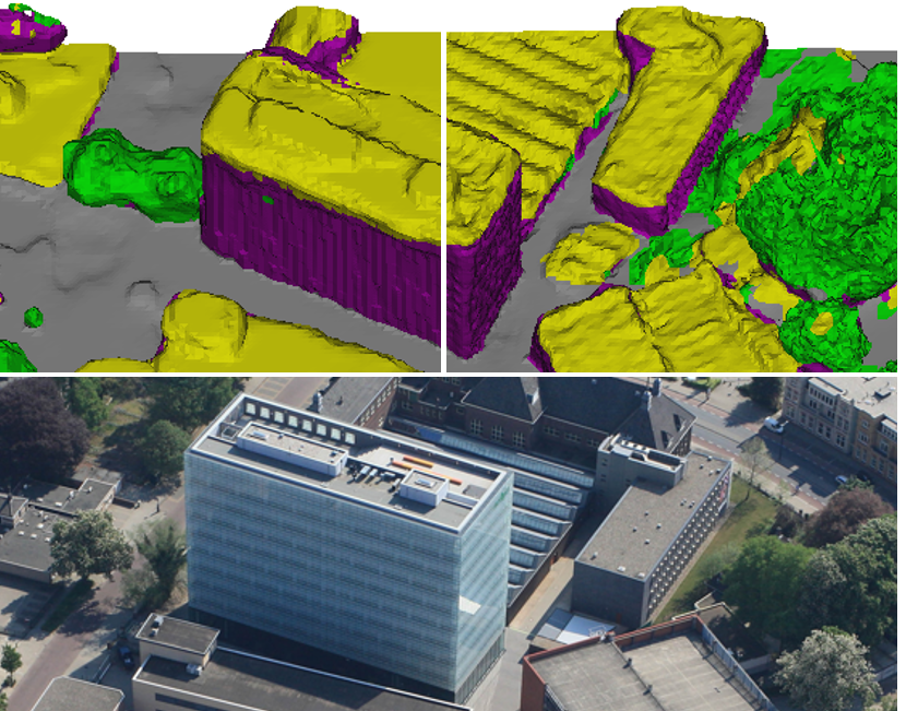
Figure 1: The impact of the proposed method. Top: labeled input model and the result after performing geometric and semantic surface refinement (left-right). Notice the higher scene fidelity - e.g. emerging structures on roofs and facades - and simultaneously an adequate, class-specific regularization in our mesh. Bottom: corresponding image.

Extracting 3D scene models from multiple images is one of the core problems in geometric computer vision. Assuming known camera poses, the problem conceptually boils down to estimating the unknown parameters of an (explicit or implicit) surface representation, such that photometric discrepancies between different views of the scene surfaces are minimized, e.g. [37]. A number of recent works have coupled the 3D reconstruction to a semantic segmentation of the scene, and have shown that, unsurprisingly, superior results can be obtained by jointly optimizing over both geometry and semantics [12, 28, 14]. A major advantage of such a semantic 3D reconstruction approach is its ability to apply class-specific priors. Any dense 3D reconstruction algorithm includes a-priori assumptions to regularize the scene geometry – in the simplest case some form of preference for smooth surfaces. Recovering a semantic segmentation together with the scene geometry makes it possible to use regularizers that are a lot more expressive, and take into account the specific geometric properties of different semantic classes. For example, one might want to selectively enforce higher smoothness on roads, where only little texture is available, or straight boundaries where building walls meet the ground.

In recent work, integrated models have been developed for semantic 3D reconstruction, but these employ a voxel-based representation of the scene which limits their resolution. Increasing the level of detail requires finer volume discretisation, which in turn increases memory consumption and computational cost, even with adaptive data structures [17, 3]. Moreover, the subsequent conversion of volumetric occupancy models to explicit surface meshes typically leads to aliasing artifacts on surfaces not aligned with the 3D coordinate system. In this work we present a scalable framework for the refinement of semantically annotated 3D surface meshes, which starts from a coarse 3D reconstruction and mitigates the mentioned limitations.

State-of-the-art techniques for reconstructing high-quality surface meshes with fine details employ a two-stage approach [25, 10, 37]. First, a coarse 3D model is generated, usually either with a volumetric approach followed by marching-cube type mesh extraction, or by triangulating the raw multi-view point cloud. The subsequent refinement improves that initial mesh by minimizing the photometric error w.r.t. the oriented images. However, existing refinement procedures are oblivious to scene semantics. The same regularization is imposed everywhere, without considering the semantic class or the presence of class transitions. Further, the result of refinement might require local semantic label changes to maintain semantic consistency.

Contributions. Here we present the first semantically informed surface refinement method for semantic 3D reconstruction. Like existing methods, ours maximizes photo-consistency to recover fine details. But it additionally exploits semantic information: (1) it also maximizes the consistency of labels across semantic segmentations of the input images; and (2) it constrains the reconstruction with shape priors that depend on the local semantic label of the surface. Our method alternates between variational optimization of the 3D surface shape and its semantic labeling using Markov Random Field inference. Consequently, our approach enables the joint refinement of two very different but mutually dependent entities for which information about one entity helps to improve the other. We show on a variety of quantitative and qualitative experiments that our approach outperforms existing methods in terms of geometric accuracy as well as semantic label accuracy.

To the best of our knowledge, we present the first mesh refinement method for 3D reconstruction which considers and jointly optimizes semantic label information in order to obtain high-resolution semantic meshes (see Fig. 1).

2 Related Work

Remarkable progress has been made in dense geometry reconstruction from images. Highly accurate 3D models can now be extracted automatically using only image data, as witnessed by the results of multiple influential benchmarks [29, 32, 5].

Although these platforms provide an extensive list of well-established techniques, methods which aim for semantic 3D reconstruction are often not present in their line-up. A possible explanation for this absence is the missing semantic ground truth. Generic benchmarking of semantic 3D models is not straightforward, as the choice of classes depends more directly on the underlying application. As an example, consider a residential area: if the goal is to check accessibility, the classification of roads is imperative, while vegetation may be less important; conversely, for urban climate or recreation, the vegetation is crucial. Despite this difficulty of finding a common target output, open semantic 3D datasets have appeared [19, 24], but so far they do not go beyond point clouds.

The topic of the present paper is at the interface of mesh refinement, mesh-based semantic segmentation and semantic 3D reconstruction. We thus review the relevant literature for these topics.

Multiview Mesh Refinement. Given an initial geometry, the common approach of variational (multi-view) mesh refinement formalizes the disagreement between the mesh and the image data in an energy function and minimizes that energy with gradient descent. Many works derive the energy in a continuous mathematical framework, e.g. [40, 11], which in principle allows one to exactly compute the gradient of the reprojection error and to properly account for visibility. Because of the discrete nature of meshes, the gradient then has to be discretized – an error-prone process. To circumvent this issue, [8] directly used the non-smooth surface for the optimization of the reprojection error. Further methods of this family are [37, 22]. Another line of work bases the refinement on patches instead of surfaces [10, 13].

To align well with the data, the energy function must measure photo-consistency as a function of the reprojected geometry [25, 37, 33]. Additionally, further visual cues can be leveraged, e.g. Lambertian surface reflectance [31, 8] or contours [33]. While these method extensions can potentially yield better 3D models, their complexity increases, with diminishing returns. In this context, [21] propose an efficient mesh refinement method that is able to determine which model-parts contribute most towards geometric fidelity, and improve only those. Finally, current research aims to simultaneously improve also the camera poses [7].

To compensate for poor evidence, such as texture-less or noisy regions, mesh fitting uses adequate regularizers. In the simplest case, they isotropically penalize strong bending of the surface, based on its principal curvatures [37]. The weight of the regularizer can be adapted to the distinctiveness of the photo-consistency metric [37]. More context-aware priors also take into account local surface noise and shape parameters within the denoising process [22].

Semantic Segmentation of Surface Meshes. State-of-the-art methods for assigning semantic labels to surface meshes are based on Conditional Random Fields (CRFs). [35] compute geometric features of the mesh in an unsupervised fashion. Per-face features form the unary potential for labeling the mesh faces with CRF inference. More related to our approach, [26, 34, 16] train classifiers for the per-face class-conditionals, using texture and/or geometric features. All those works combine the per-face unary potential with a generic, pairwise smoothness term. On the contrary, we additionally employ geometric surface information within the labeling process. Related work on CRF-based mesh labeling in the context of mesh texturing was presented in [38, 20].

Semantic 3D Reconstruction. The goal to jointly infer 3D shape and object classes in a principled manner, by fitting a coupled model, was initially tackled in [18]. That work was still formulated in 2.5D using depth maps. True 3D methods appeared only recently, mostly with volumetric representations [12, 1, 28, 27]. The methods were extended to handle city-scale models [17, 3, 36]; large label sets, also in urban scenes [6]; and thin semantic layers like hair on human heads [23]. Departing from the volumetric approach, [4] do semantic 3D reconstruction with a (low-resolution) triangle mesh. The common ground of all these works is that they allow local shape to influence the appearance-based class labels and vice versa, via class-specific regularization.

Relation to our Work. To the best of our knowledge, none of the existing mesh refinement approaches specifically utilizes semantic labels to impose class-specific shape knowledge. And vice versa, none of the semantic 3D reconstruction techniques applies mesh refinement to obtain a model with the amount of surface detail present in high-resolution 3D models. This gap is the starting point for our work.

3 Method

We assume as given a set of calibrated cameras, for which we have both the intensity images and the semantic segmentations, in the form of pixel-wise likelihoods for all possible classes. Furthermore, we assume there is an initial surface mesh, e.g., from structure-from motion or coarse semantic 3D reconstruction. The mesh also has per-face semantic labels – if this is not the case, they can easily be generated by projecting the per-image class scores onto the surface and aggregating them with some consensus mechanism. Our goal is to move the vertices of the initial mesh, and to change the semantic labels of its faces, until the consistency between the images is maximized w.r.t. both photometry and semantic segmentation. Additionally, we define a set of priors that link geometric shape to semantic class, and constrain the refinement.

To obtain a tractable algorithm, we split the optimization into two subproblems, which we then solve independently in an alternating manner. 1) One optimization updates the geometry while keeping the labels fixed. In that step, the (fixed) labels induce class-specific priors in the shape, such as for example that building walls tend to be smoother than vegetation. 2) The other optimization relabels the mesh faces, while keeping the geometry fixed. In that step the surface shape serves as prior that influences the labeling, e.g. vertical faces prefer to be labeled as building walls.

For the geometric update, we employ a variational mesh refinement scheme [25, 37], which we extend to include semantic labels.

The class-specific priors in volumetric reconstruction schemes seek to constrain surface orientation [12, 28, 3, 23]. This might interfere with the goal of retrieving high detailed surface geometry. In contrast, we leverage the surface curvature and wish to make the strength of the smoothness prior dependent on the semantic class (e.g., high for road, low for vegetation). Further, we want to favor certain edge orientations for faces along class transitions.

For the semantic relabeling, we work on the graph implied by the surface mesh and rely on standard CRF inference. As feedback from the surface geometry, we include a term that depends on the face’s normal vector, so as to favor labels that are consistent with the surface orientation. Empirically the alternation quickly converges to a stable state of labeling and the geometry.

3.1 Variational Surface Refinement

The surface $S$ is parametrized as a labeled triangle mesh, represented by the tuple $(\mathcal{V},\mathcal{F},\mathcal{F}^{l})$ of vertices $\mathcal{V}$, faces $\mathcal{F}$, and per-face semantic labels $\mathcal{F}^{l}$. Like most other refinement algorithms we assume that (1) the topology of the initial mesh does not change during refinement, and (2) the mesh lies close enough to the true surface to employ local, gradient-based optimization. The surface is observed by $n$ cameras with known projections $\Pi_{i}:\mathbb{R}^{3}\rightarrow\mathbb{R}^{2}$, and associated images $I_{i}:\Omega_{i}\subset\mathbb{R}^{2}\rightarrow\mathbb{R}^{d}$ with $d\in\{1,3\}$ color channels. Furthermore, all input images have been segmented with a semantic per-pixel classifier into a set of $\mathcal{L}=\{1,\ldots,L\}$ different labels. The corresponding likelihood images for each label $l$ are denoted as $I^{l}_{i}:\Omega_{i}\rightarrow[0,1]$.

Similar to [37], we compute the refined surface $S$ as the minimizer of a variational energy, made up of a data and smoothness terms:

$$E(S)=\underbrace{E_{\text{photo}}+\lambda_{1}E_{\text{sem}}}_{\text{data consistency}}+\underbrace{\lambda_{2}E_{\text{intra}}+\lambda_{3}E_{\text{inter}}}_{\text{smoothness}}\enspace.$$ (1)

The weights $\lambda_{1},\lambda_{2},\lambda_{3}\in\mathbb{R}_{\geq 0}$ define the relative impact of each individual term. The variation of this energy corresponds to a vector field along the surface, which is used to iteratively deform the mesh via gradient descent, until convergence. The data term is divided into a photo-consistency and a semantic consistency term. Likewise, the smoothness terms incorporate priors for semantic intra-class and inter-class dependencies. In the following we detail each term individually.

3.2 Data Consistency

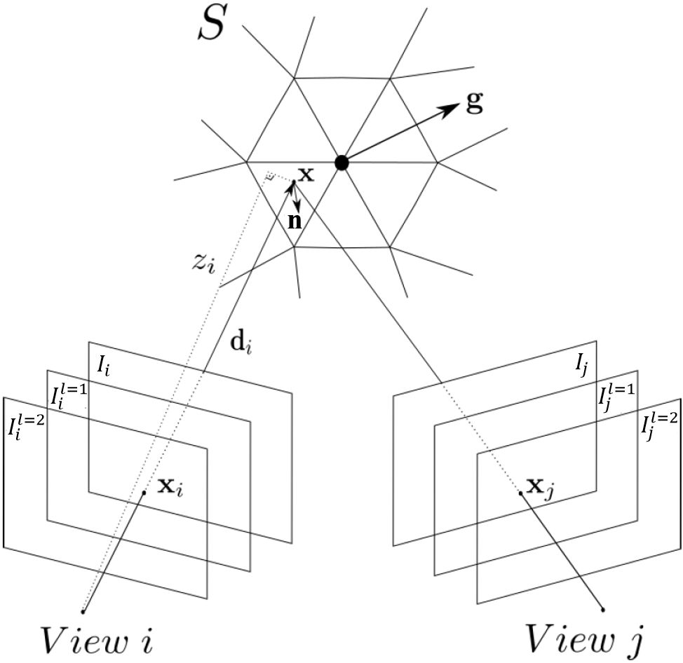
Figure 2: Illustration of the reprojection.

We enforce consistency with the input data by two separate energy terms. One promotes photometric consistency with the images, the other semantic consistency with the 2D label maps.

Photometric Consistency. The photo-consistency term minimizes the photometric reprojection error between pairs of camera images. Similar to [37] we defined it as

$$E_{\text{photo}}(S)=\sum_{i,j}\int_{\Omega_{ij}}h\big{(}I_{i},I_{ij}\big{)}(x_{i})\;dx_{i}\enspace,$$ (2)

where the function $h(I_{i},I_{ij})(x_{i})$ measures the photo-consistency between image $I_{i}$ and $I_{j}$ at pixel $x_{i}$, and $I_{ij}=I_{j}\circ\Pi_{j}\circ\Pi_{i}^{-1}$ is the reprojection of image $I_{j}$ into image $I_{i}$ via the surface $S$ and is depicted in Fig. 2. The corresponding image domain $\Omega_{ij}\subset\Omega_{i}$ is induced by the reprojection of image $I_{j}$. The energy gradient is given by

$$\frac{dE_{\text{photo}}(S)}{dX} =\sum_{i,j}\int_{\Omega_{ij}}\phi(x)f_{ij}(x_{i})/(\mathbf{n}^{T}\mathbf{d}_{i})\mathbf{n}\;dx_{i}$$ (3)

$$f_{ij}(x_{i}) =\partial_{2}M(x_{i})DI_{j}(x_{j})D\Pi_{j}(x)\mathbf{d}_{i}\enspace,$$ (4)

in which function $\phi(x)$ weighs the pixels in the back-projected triangles that contain vertex $x$ according to the barycentric triangle coordinates. Furthermore, $\mathbf{n}$ is the surface normal, $\mathbf{d}_{i}$ the distance from the camera center to the point on the surface, symbol $D$ denotes the Jacobian of a function, and $\partial_{2}M$ is the derivative of the similarity measure w.r.t. its second argument. For the similarity measure $h(\cdot)$, we use zero-mean normalized cross-correlation. In practice this term enhances the reconstruction of fine details, but also introduces geometric noise without additional regularization [37].

Semantic Consistency. In the same spirit, the semantic consistency term minimizes the discrepancies between pairs of 2D semantic segmentation maps corresponding to different input views. While accounting for all cameras pairs $i,j$ and all labels $l\in\mathcal{L}$, the following term measures pixel-wise differences of class-likelihoods between the two semantic segmentation maps $I^{l}_{i}$ and $I^{l}_{j}$

$$E_{\text{sem}}(S)=\sum_{l\in\mathcal{L}}\sum_{i,j}\int_{\Omega_{ij}}\frac{1}{2}\big{(}I^{l}_{i}(x_{i})-I^{l}_{ij}(x_{i})\big{)}^{2}\;dx_{i}\enspace.$$ (5)

This term and its derivative is identical to Eq. (3) with the difference that the similarity measure $h(\cdot)$ is the sum of squared differences and the comparison is done between label likelihoods instead of color values.

3.3 Smoothness of Geometry

Smoothness of the refined surfaces is encouraged by two terms, one for intra-class, and one for inter-class regularity.

Intra-class Smoothness. Here we use the classical thin-plate minimal curvature regularization, generalized for the multi-class setting. In this way, we can enforce different levels of smoothness for different classes. For instance, facades are in general smoother than vegetation. Furthermore, class transitions mostly coincide with high surface curvature (e.g. from ground to building). Consequently, we introduce a smoothing weight for each class and our intra-class smoothness term reads as

$$E_{\text{intra}}(S)=\sum_{l\in\mathcal{L}}\sum_{\mathbf{v}\in\mathcal{V}_{l}}\omega_{l}\frac{1}{2}\Big{(}\kappa_{1}(\mathbf{v})+\kappa_{2}(\mathbf{v})\Big{)}\enspace,$$ (6)

where $\mathcal{V}_{l}\subset\mathcal{V}$ corresponds to vertices that encompass a semantically homogeneous one-ring-neighborhood with label $l$, and $\omega_{l}$ a class-specific weight factor. Note that this regularizer can easily be extended to include image-based information, e.g. adapt the amount of smoothing along edges in the input image, as they often align with object edges (as for example done in [39]).

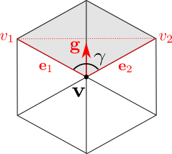
Figure 3: Top view on a two-label one-ring-neighborhood of $\mathbf{v}$. Visualization of the construction of the gradient vector $\mathbf{g}$ used for forcing smooth transition boundaries.

Inter-class Smoothness. The inter-class smoothness accounts for regularity along class boundaries. On a discrete mesh, these boundaries are represented by sequences of adjacent edges, each adjoining two faces with different labels. To enforce smoothness of these boundaries, we penalize angular deviations along class transitions by minimizing the energy

$$E_{\text{inter}}(S)=\sum_{\mathbf{v}\in\mathcal{V}_{T}}(\pi-\gamma(\mathbf{v}))^{2}\enspace,$$ (7)

in which $\mathcal{V}_{T}\subset\mathcal{V}$ is the set of vertices featuring a two-label one-ring-neighborhood, where faces with equal labels are direct neighbors. Class transitions in such a triangle fan are defined by two edges $\mathbf{e}_{1}$, $\mathbf{e}_{2}$ and the corresponding vertices $\mathbf{v}$, $\mathbf{v}_{1}$, $\mathbf{v}_{2}$, see Fig. 3. The energy of Eq. (7) is minimal if the angle $\gamma(\mathbf{v})$ between $\mathbf{e}_{1}$ and $\mathbf{e}_{2}$ is $\pi$. Note that in the current definition we do not consider triangle fans with more than two labels because a separate modeling of these rare cases is not beneficial.

Discussion. When all semantically related terms and relations are neglected, i.e. we consider only one label, the intra-class smoothness term in Eq. (6) simplifies to

$$E_{\text{smooth}}(S)=\sum_{\mathbf{v}\in\mathcal{V}}\frac{1}{2}\Big{(}\kappa_{1}(\mathbf{v})+\kappa_{2}(\mathbf{v})\Big{)}\enspace,$$ (8)

with $\kappa_{1}(\mathbf{v})$ and $\kappa_{2}(\mathbf{v})$ being the principal curvatures at vertex $\mathbf{v}$. Together with the remaining photo-consistency term in Eq. (2) the overall energy reduces to

$$E_{\text{baseline}}(S)=E_{\text{photo}}(S)+\lambda E_{\text{smooth}}(S)\enspace.$$ (9)

The minimization of this simplified energy corresponds to the purely geometric refinement method described in [37], which we use as baseline for comparisons. Our geometry refinement can be seen as generalization of [37] that incorporates semantic labels and a corresponding set of rich, semantic priors which allow to favor different class-dependent surface properties.

Minimization. The sum of the derivatives of all energy terms defines for each vertex a 3D direction in which it should be moved to improve the energy. Together with a fixed step width this defines a single gradient descent step which we iterate until convergence in alternation with the semantic relabeling.

3.4 Semantic Relabeling

The variational surface refinement changes the mesh geometry. As individual faces move, their labels may become inconsistent with those given by the 2D semantic likelihoods of the input images. In order to minimize such inconsistencies we relabel the faces after a fixed number of geometric refinement iterations. The relabeling is formulated as an energy minimization in a Markov Random Field. Each face corresponds to a node in the MRF graph, sharing three node interactions with its adjacent faces. Let $\mathcal{F}$ be the set of faces and $\mathcal{L}$ the set of potential class labels. The goal is to derive a labeling $\mathbf{l}\in\mathcal{F}^{l}$ that assigns a label $l_{f}\in\mathcal{L}$ to each face $f\in\mathcal{F}$, such that the energy $E(\mathbf{l})$ is minimized. More precisely, our energy has the form

$$E(\mathbf{l}) =\sum_{f\in\mathcal{F}}E_{\text{data}}(l_{f})+\mu_{1}\sum_{f\in\mathcal{F}}E_{\text{geo}}(\mathbf{n}_{f},l_{f})$$

$$+\mu_{2}\sum_{f\in\mathcal{F},g\in\mathcal{N}_{f}}E_{\text{smooth}}(l_{f},l_{g})\enspace,$$ (10)

where the weights $\mu_{1},\mu_{2}$ control the contribution of the label-dependent geometry prior $E_{\text{geo}}$ and the label smoothness prior $E_{\text{smooth}}$. The data term

$$E_{\text{data}}(l_{f})=-\log\left(\sum_{i}\int_{\Psi_{i}}I^{l_{f}}_{i}(x_{i})\;dx_{i}\right)$$ (11)

integrates the likelihoods of class $l_{f}$ in the likelihood images $I_{i}^{l_{f}}$. Per image, integration is carried out over the domain $\Psi_{i}$, defined by the area of the reprojected face. Note that by integration in image space we exploit the same benefits as during geometric refinement: we put emphasis on large faces and images close to the surface, while reducing the influence of observations from slanted viewing angles.

Analogous to the use of semantically modulated priors during geometric refinement, we now employ a geometry-dependent prior for the mesh labeling. In this way we retain a tight coupling between the semantic and geometric optimization steps. The prior is dependent on the face normal and penalizes class labels which contradict the surface orientation. For example, labeling a face with vertical normal as a facade would induce a higher cost than assigning it the class ground. Due to the wide range of possible normals of our classes (ground, facade, roof, vegetation), we found it best to define individual penalties as conservatively parametrized step functions:

$$E_{\text{geo}}(\mathbf{n}_{f},l_{f})=\begin{cases}A_{f}\quad\text{if}\quad\|\measuredangle(\mathbf{n}_{f},\mathbf{n}_{z})-\beta(l_{f})\|>\alpha(l_{f})\\ 0\quad\text{otherwise}\end{cases}\enspace.$$ (12)

Here $\mathbf{n}_{z}$ corresponds to the gravity vector (typically $(0,0,1)^{T}$), $\mathbf{n}_{f}$ is the face normal and $A_{f}$ is the triangle size, to account for the surface area. The parameter $\beta$ specifies the ideal (set of) class-wise normal(s) expressed with respect to $\mathbf{n}_{z}$. The parameter $\alpha$ determines the range of angles for which penalties are imposed. The parameters used in our experiments are given in Table 1.

Given a face $f$, and another face $g$ in its one-ring neighborhood $\mathcal{N}_{f}$, the pair-wise smoothness term is defined as

$$E_{\text{smooth}}(l_{f},l_{g})=\begin{cases}A_{f}\quad\text{if}\quad l_{g}\neq l_{f}\\ 0\quad\text{otherwise}\end{cases}.$$ (13)

As before, the triangle area $A_{f}$ serves as weight to increase contributions of larger triangles.

To find a (local) minimum of $E(\mathbf{l})$ we run loopy belief propagation [9]. In all experiments we set $\mu_{1}=0.35$, $\mu_{2}=0.5$.

	roof	vegetation	ground	facade
$\alpha(l_{f})[^{\circ}]$	60	180	30	30
$\beta(l_{f})[^{\circ}]$	0	0	0	90

Table 1: Parameters of class-dependent geometric prior.

4 Experiments

All experiments were performed on a machine with 64 GB of RAM and a 12-core Intel Xeon E5 CPU at 2.7 GHz. We start with a quantitative evaluation on a synthetic scene, and then go on to reconstruct four challenging real world scenarios featuring different sensors and camera network configurations.

Data. The processed datasets comprise vertical and oblique aerial views of urban areas, as well as a terrestrial outdoor scenario. For a quantitative verification and a comparison to state-of-the-art methods, we process SynthCity3 from [4], for which a labeled ground truth model is available. To test our algorithm on real world data, we further process three image sets covering Enschede (Netherlands)[30], Dortmund (Germany)[15] and Southbuilding (Fig. 5). For the very large SynthCity3 and Enschede datasets we process two sub-patches (in the following referred to as SynthCity3 A/B and Enschede A/B). For the real-world scenarios, geometric ground truth is not available. However, to quantitatively check the correctness of our models, we render the surface semantics and compare the results to hand-labeled, semantic ground truth images. Tab. 2 shows the characteristics of the input data at a glance.

Our algorithm requires three types of inputs: (1) intensity images, i.e. RGB or grayscale, (2) semantic segmentation maps of those images with a per-pixel likelihood for each class, and (3) an initial, semantically annotated 3D surface with consistent topology. The semantic segmentations (2) are obtained from a MultiBoost classifier [2] trained on a few manually labeled images. For our scenarios, we choose four mutually exclusive labels: ground, facade, roof and vegetation. The input surface (3) is generated using the semantic 3D reconstruction of [3], followed by marching-cube mesh conversion. Fig. 4 illustrates a sample of our input data from the Enschede data set.

Data set	Resolution [pix]	GSD [m]	# of images
SynthCity3 A	1416 x 1062	N/A	15
SynthCity3 B	1416 x 1062	N/A	15
Enschede A	1404 x 936	0.4	15
Enschede B	1404 x 936	0.4	14
Dortmund	1363 x 1020	0.60	12
Southbuilding	768 x 576	N/A	15

Table 2: Technical specifications of the processed image sets. The GSD corresponds to the average pixel footprint of the vertical and oblique aerial images. In SynthCity A and B, this value has no metric unit. In the terrestrial Southbuilding images, it varies greatly across the scene.

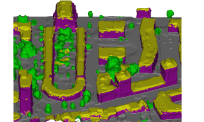
Figure 4: Input data of our algorithm (Enschede A), comprising intensity images (grayscale or RGB), semantic segmentation maps and an initial semantic 3D model with consistent topology (left-to-right). The segmentation map is visualized by the class with maximum likelihood among: ground (gray), facade (purple), roof (yellow), vegetation (green).

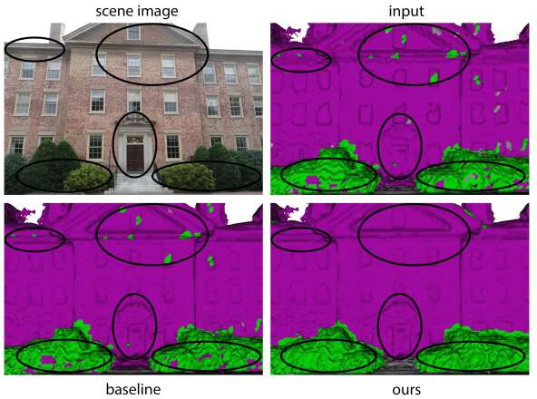
Figure 5: Results of the terrestrial Southbuilding data set. The proposed method outperforms our input [3] and baseline [37] model. Exemplary improvements are highlighted with black circles.

Quantitative Evaluation. We evaluate our method in terms of geometric and semantic accuracy. As baseline, we use our own reimplementation of the state-of-the-art algorithm for mesh refinement [37]. Further, the proposed approach can generally be considered as a post-processing step for semantic 3D modeling algorithms like [12, 3, 28, 27]. For this reason, we also compare against our initialization, the output of [3].

In terms of geometry, we are interested in two aspects: how much is the overall improvement compared to the input model, and how do we perform against the baseline mesh refinement? The first aspect confirms the need for refinement after semantic 3D reconstruction, and at the same time checks whether the input mesh is good enough to serve as starting value for local optimization. The second comparison assesses our contribution, answering the question: Does the semantic information improve the mesh? Moreover, checking the semantic correctness verifies if the geometry refinement and input likelihoods can be leveraged for semantic relabeling.

For geometric verification we use SynthCity3 A and B. Each of those represents a building block of an urban scenario. For a fair comparison, we first empirically determine the parameters of the baseline that lead to the most accurate 3D model. This configuration is then fixed, and only the parameters of our additional semantic terms are changed for further fine-tuning. Finally, we run five iterations for both methods. Per iteration, we perform a geometric update for the baseline, and a sequential geometric and semantic update for our method. Our method achieves the highest geometric accuracy in this test (Tab. 3). Due to the synthetic nature of the reference model, the values are relative. To augment them with an absolute metric unit, we measure and average the dimensions of comparable real world city blocks, and scale our models accordingly.

In contrast to geometry, the semantic correctness of real-world models was quantitatively checked for all scenes. To obtain ground truth data, we select a representative image in each scenario and manually label it. The semantic 3D reconstructions are then projected, and compared to the ground truth in terms of average accuracy and overall accuracy. This procedure is illustrated for the Enschede B data set in Fig. 6. Tab. 3 summarizes the numeric results. Again, we outperform our input and baseline method in all data sets.

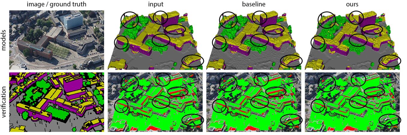
Figure 6: Quantitative evaluation of the semantic correctness (Enschede B). Top: scene image, input model [3], baseline model [37], ours (left-to-right). Bottom: ground truth, error plot input, error plot baseline, error plot ours. Misclassified pixels are shown in red. Exemplary improvements are highlighted with black circles.

Data set	Modality	Performance Measure	[3]	[37]	Ours
SynthCity3 A	Geometry	Mean distance to ground truth [relative]	0.0076	0.0064	0.0055
		Mean distance to ground truth [m]	0.52	0.44	0.38
	Semantics	Average accuracy [%]	82.6	82.8	88.8
		Overall accuracy [%]	85.2	85.6	86.1
SynthCity3 B	Geometry	Mean distance to ground truth [relative]	0.0121	0.0107	0.0090
		Mean distance to ground truth [m]	0.84	0.74	0.62
	Semantics	Average accuracy [%]	83.6	83.8	90.0
		Overall accuracy [%]	86.2	86.5	88.7
Enschede A (Netherlands)	Semantics	Average accuracy [%]	78.8	78.8	83.3
		Overall accuracy [%]	82.6	82.7	85.2
Enschede B (Netherlands)	Semantics	Average accuracy [%]	89.5	89.7	93.5
		Overall accuracy [%]	90.4	90.6	94.1
Dortmund (Germany)	Semantics	Average accuracy [%]	86.5	86.6	87.6
		Overall accuracy [%]	92.3	92.4	92.7
Southbuilding	Semantics	Average accuracy [%]	81.9	78.7	94.5
		Overall accuracy [%]	93.8	93.8	98.0

Table 3: Quantitative evaluation of our method. Best performance is shown in bold.

Qualitative Evaluation. Jointly exploiting geometry and semantics during the surface refinement allows for a more steerable procedure. The additional degrees of freedom can be leveraged to obtain qualitatively better results, as we will demonstrate on the basis of an urban test scenario (Fig. 7). The class facade appears vertical and flat in our input models and suffers from aliasing, due to the preceding volumetric representation. In contrary, our method recovers fine structures (e.g. windows), removes artifacts and performs adequate smoothing. For the second class vegetation, trees appear as blobs in our initial geometry. Due to the highly undulated surface structure of trees within our method smoothness regularization is limited to a large degree and we strive for high data alignment. This leads to more realistic reconstructions of vegetation areas. Finally, we decide to keep geometry annotated by the class ground close to the highly regularized input models for the following reasons: (1) refining the geometry would mostly reconstruct cars which are dynamic objects and not of interest in terms of the static scene; (2) the ground does only suffer minor aliasing artifacts, since the scenes are aligned with the gravity vector.

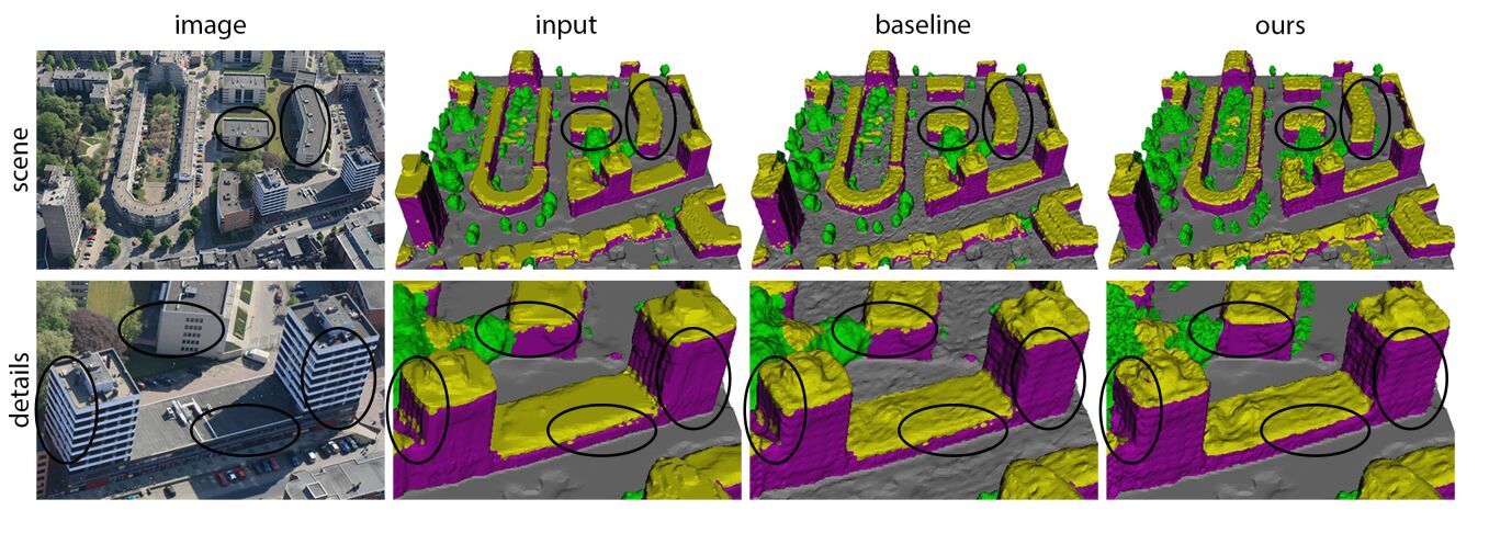
Figure 7: Qualitative evaluation of our method based on models of the Enschede A data set (top) and corresponding details (bottom). Left-to-right: Input model [3], baseline model [37], ours. Notice the high scene fidelity, and, at the same time an adaptive, class-specific surface regularization, clean class transitions and less noisy semantics in our model. Exemplary improvements are highlighted with black circles.

Beyond Aerial Reconstruction. 3D reconstruction of urban habitates from aerial data is a major application of 3D modeling and scene interpretation from images today, which was the reason and motivation to test our method primary on these type of data. However, to show the versatility of the proposed method we additionally perform an evaluation on the terrestrial Southbuilding dataset, featuring very different sensor and scene characteristics. As for the aerial settings, we outperform our input and the baseline method. Tab. 3 summarizes the quantitative results, Fig. 5 show visual differences.

5 Conclusion

We proposed a method for the joint geometric and semantic refinement of labeled 3D surfaces meshes. Our algorithm leverages photometric and semantic image information in an integrated manner to refine the geometry of an inital surface mesh. Furthermore, we exploit semantic information for class-aware regularization within geometric refinement, and use geometric shape to improve the semantic labeling. Our optimization scheme alternates between variational surface refinement and MRF inference for relabeling. In a broad sense, our method corresponds to a generalization of pure geometric surface refinement, which incorporates semantic labels and a rich set of corresponding semantic priors. At the same time it can be seen as a multi-view consistent semantic segmentation in 3D. Combining both aspects leads to superior, more detailed and interpreted 3D models.

Our method is not limited to outdoor views of urban scenes, like those tested within this paper. In future work, we would like to experiment with different types of data, such as imagery of indoor scenarios. As the scene characteristics and data quality varies greatly across different test beds and sensors, we would like to explore methods for data-driven, automatic balancing of the individual terms in our framework.

References

- [1] S. Y. Bao, M. Chandraker, Y. Lin, and S. Savarese. Dense object reconstruction with semantic priors. CVPR, 2013.
- [2] D. Benbouzid, R. Busa-Fekete, N. Casagrande, F.-D. Collin, and B. Kégl. Multiboost: a multi-purpose boosting package. JMLR, 2012.
- [3] M. Bláha, C. Vogel, A. Richard, J. D. Wegner, T. Pock, and K. Schindler. Large-scale semantic 3d reconstruction: an adaptive multi-resolution model for multi-class volumetric labeling. CVPR 2016.
- [4] R. Cabezas, J. Straub, and J. W. Fisher III. Semantically-aware aerial reconstruction from multi-modal data. ICCV, 2015.
- [5] S. Cavegn, N. Haala, S. Nebiker, M. Rothermel, and P. Tutzauer. Benchmarking high density image matching for oblique airborne imagery. ISPRS Technical Commission III Symposium, 2014.
- [6] I. Cherabier, C. Häne, M. R. Oswald, and M. Pollefeys. Multi-label semantic 3d reconstruction using voxel blocks. 3DV, 2016.
- [7] A. Delaunoy and M. Pollefeys. Photometric bundle adjustment for dense multi-view 3d modeling. CVPR, 2014.
- [8] A. Delaunoy, E. Prados, P. Gargallo, J.-P. Pons, and P. Sturm. Minimizing the multi-view stereo reprojection error for triangular surface meshes. BMVC, 2008.
- [9] B. J. Frey and D. J. MacKay. A Revolution: Belief Trees: Belief Propagation in Graphs With Cycles. In M. I. Jordan, M. J. Kearns, and S. A. Solla, editors, Advances in Neural Information Processing Systems. MIT Press, Cambridge, MA, 1998.
- [10] Y. Furukawa and J. Ponce. Accurate, dense, and robust multi-view stereopsis. PAMI, 1(1), 2008.
- [11] P. Gargallo, E. Prados, and P. Sturm. Minimizing the reprojection error in surface reconstruction from images. ICCV, 2007.
- [12] C. Häne, C. Zach, A. Cohen, R. Angst, and M. Pollefeys. Joint 3d scene reconstruction and class segmentation. CVPR, 2013.
- [13] P. Heise, B. Jensen, S. Klose, and A. Knoll. Variational patchmatch multiview reconstruction and refinement. ICCV, 2015.
- [14] S. Ikehata, H. Yan, and Y. Furukawa. Structured Indoor Modeling. ICCV, 2015.
- [15] ISPRS / EuroSDR Benchmark for Multi-Platform Photogrammetry. http://www2.isprs.org/commissions/comm1/icwg15b/benchmark_main.html.
- [16] E. Kalogerakis, A. Hertzmann, and K. Singh. Learning 3d mesh segmentation and labeling. In ACM SIGGRAPH 2010 Papers, pages 102:1–102:12, 2010.
- [17] A. Kundu, Y. Li, F. Daellert, F. Li, and J. M. Rehg. Joint semantic segmentation and 3d reconstruction from monocular video. ECCV, 2014.
- [18] L. Ladicky, P. Sturgess, C. Russel, S. Sengupta, , Y. Bastanlar, W. Clocksin, and P. Torr. Joint optimisation for object class segmentation and dense stereo reconstruction. BMVC, 2010.
- [19] Large-Scale Point Cloud Classification Benchmark. http://www.semantic3d.net/.
- [20] V. Lempitsky and D. Ivanov. Seamless mosaicing of image-based texture maps. In CVPR, pages 1–6, 2007.
- [21] S. Li, S. Y. Siu, T. Fang, and L. Quan. Efficient multi-view surface refinement with adaptive resolution control. ECCV, 2016.
- [22] Z. Li, K. Wang, W. Zuo, D. Meng, and L. Zhang. Detail-preserving and content-aware variational multi-view stereo reconstruction. arXiv, abs/1505.00389, 2015.
- [23] F. Maninchedda, C. Häne, B. Jacquet, A. Delaunoy, and M. Pollefeys. Semantic 3d reconstruction of heads. ECCV, 2016.
- [24] NYU Depth Dataset. http://cs.nyu.edu/~silberman/datasets/nyu_depth_v2.html.
- [25] J.-P. Pons, R. Keriven, and O. Faugeras. Multi-view stereo reconstruction and scene flow estimation with a global image-based matching score. IJCV, 72(2), 2007.
- [26] M. Rouhani, F. Lafarge, and P. Alliez. Semantic segmentation of 3d textured meshes for urban scene analysis. {ISPRS} Journal of Photogrammetry and Remote Sensing, 123:124 – 139, 2017.
- [27] N. Savinov, C. Häne, L. Ladicky, and M. Pollefeys. Semantic 3d reconstruction with continuous regularization and ray potentials using a visibility consistency constraint. In CVPR, pages 5460–5469, 2016.
- [28] N. Savinov, L. Ladicky, C. Häne, and M. Pollefeys. Discrete optimization of ray potentials for semantic 3d reconstruction. CVPR, 2015.
- [29] S. M. Seitz, B. Curless, J. Diebel, D. Scharstein, and R. Szeliski. A comparison and evaluation of multi-view stereo reconstruction algorithms. CVPR, 2006.
- [30] Slagboom en Peeters Aerial Survey. http://www.slagboomenpeeters.com/3d.htm.
- [31] S. Soatto, A. J. Yezzi, and H. Jin. Tales of shape and radiance in multi-view stereo. ICCV, 2003.
- [32] C. Strecha, W. V. Hansen, L. J. V. Gool, P. Fua, and U. Thoennessen. On benchmarking camera calibration and multi-view stereo for high resolution imagery. CVPR, 2008.
- [33] R. Tyleček and R. Šara. Refinement of surface mesh for accurate multi-view reconstruction. Virtual Reality, 9, 2010.
- [34] J. P. C. Valentin, S. Sengupta, J. Warrell, A. Shahrokni, and P. H. S. Torr. Mesh based semantic modelling for indoor and outdoor scenes. In CVPR, pages 2067–2074, 2013.
- [35] Y. Verdie, F. Lafarge, and P. Alliez. Lod generation for urban scenes. ACM Trans. Graph., pages 30:1–30:14, 2015.
- [36] V. Vineet, O. Miksik, M. Lidegaard, M. Niessner, and S. Golodetz. Incremental dense semantic stereo fusion for large-scale semantic scene reconstruction. ICRA, 2015.
- [37] H. H. Vu, P. Labatut, J.-P. Pons, and R. Keriven. High accuracy and visibility-consistent dense multiview stereo. PAMI, 34(5), 2012.
- [38] M. Waechter, N. Moehrle, and M. Goesele. Let there be color! large-scale texturing of 3d reconstructions. In ECCV, pages 836–850, 2014.
- [39] C. Wu, B. Wilburn, Y. Matsushita, and C. Theobalt. High-quality shape from multi-view stereo and shading under general illumination. In CVPR, pages 969–976, 2011.
- [40] A. Yezzi and S. Soatto. Stereoscopic segmentation. IJCV, 53(1), 2003.