Compressed Factorization: Fast and Accurate
Low-Rank Factorization of Compressively-Sensed Data

Abstract

What learning algorithms can be run directly on compressively-sensed data? In this work, we consider the question of accurately and efficiently computing low-rank matrix or tensor factorizations given data compressed via random projections. We examine the approach of first performing factorization in the compressed domain, and then reconstructing the original high-dimensional factors from the recovered (compressed) factors. In both the matrix and tensor settings, we establish conditions under which this natural approach will provably recover the original factors. While it is well-known that random projections preserve a number of geometric properties of a dataset, our work can be viewed as showing that they can also preserve certain solutions of non-convex, NP-Hard problems like non-negative matrix factorization. We support these theoretical results with experiments on synthetic data and demonstrate the practical applicability of compressed factorization on real-world gene expression and EEG time series datasets.

1 Introduction

We consider the setting where we are given data that has been compressed via random projections. This setting frequently arises when data is acquired via compressive measurements (Donoho, 2006; Candès and Wakin, 2008), or when high-dimensional data is projected to lower dimension in order to reduce storage and bandwidth costs (Haupt et al., 2008; Abdulghani et al., 2012). In the former case, the use of compressive measurement enables higher throughput in signal acquisition, more compact sensors, and reduced data storage costs (Duarte et al., 2008; Candès and Wakin, 2008). In the latter, the use of random projections underlies many sketching algorithms for stream processing and distributed data processing applications (Cormode et al., 2012).

Due to the computational benefits of working directly in the compressed domain, there has been significant interest in understanding which learning tasks can be performed on compressed data. For example, consider the problem of supervised learning on data that is acquired via compressive measurements. Calderbank et al. (2009) show that it is possible to learn a linear classifier directly on the compressively sensed data with small loss in accuracy, hence avoiding the computational cost of first performing sparse recovery for each input prior to classification. The problem of learning from compressed data has also been considered for several other learning tasks, such as linear discriminant analysis (Durrant and Kabán, 2010), PCA (Fowler, 2009; Zhou and Tao, 2011; Ha and Barber, 2015), and regression (Zhou et al., 2009; Maillard and Munos, 2009; Kabán, 2014).

Building off this line of work, we consider the problem of performing low-rank matrix and tensor factorizations directly on compressed data, with the goal of recovering the low-rank factors in the original, uncompressed domain. Our results are thus relevant to a variety of problems in this setting, including sparse PCA, nonnegative matrix factorization (NMF), and Candecomp/Parafac (CP) tensor decomposition. As is standard in compressive sensing, we assume prior knowledge that the underlying factors are sparse.

For clarity of exposition, we begin with the matrix factorization setting. Consider a high-dimensional data matrix $M\in\mathbb{R}^{n\times m}$ that has a rank-$r$ factorization $M=WH$, where $W\in\mathbb{R}^{n\times r}$, $H\in\mathbb{R}^{r\times m}$, and $W$ is sparse. We are given the compressed measurements $\tilde{M}=PM$ for a known measurement matrix $P\in\mathbb{R}^{d\times n}$, where $d<n$. Our goal is to approximately recover the original factors $W$ and $H$ given the compressed data $\tilde{M}$ as accurately and efficiently as possible.

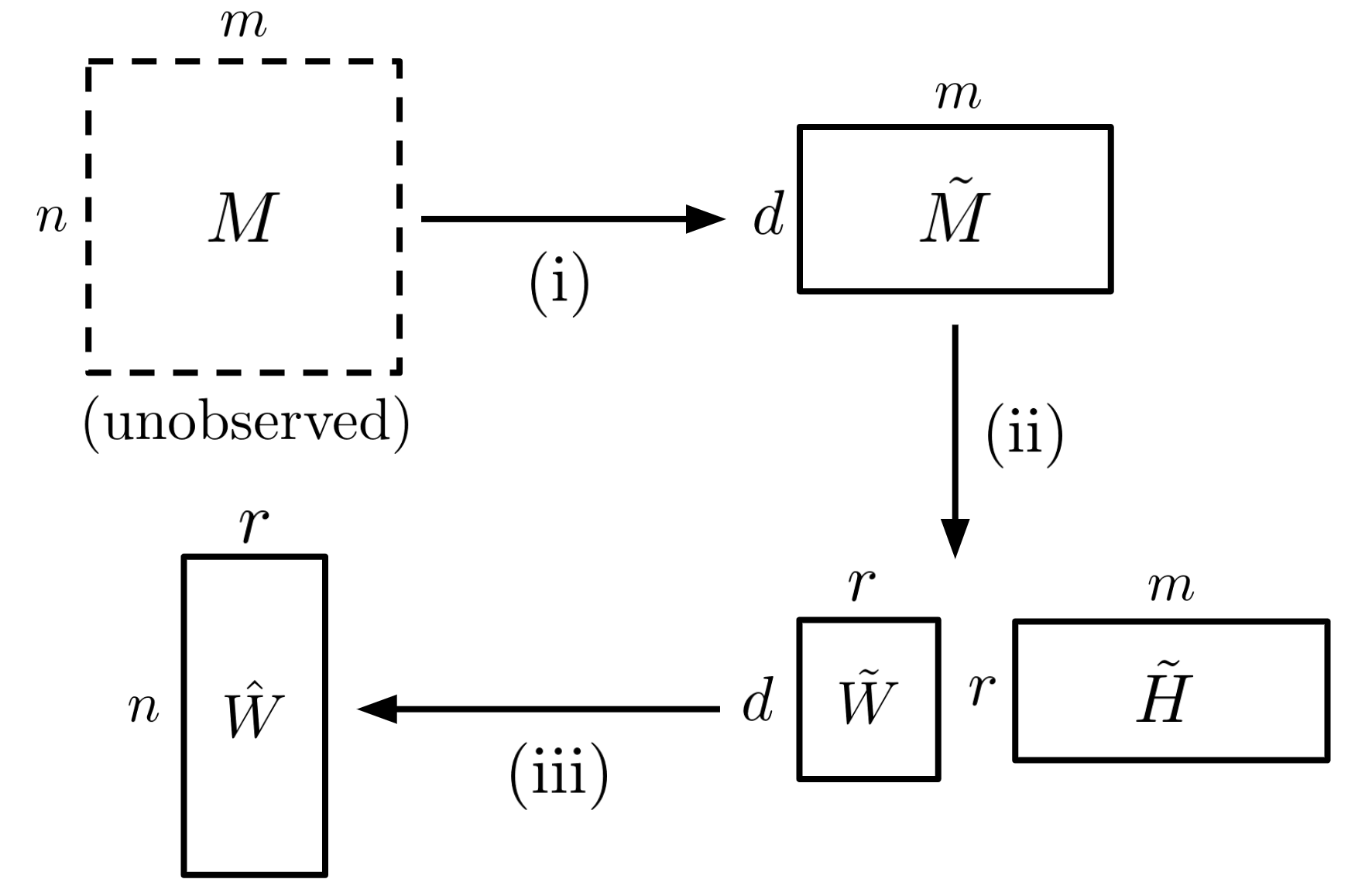
Figure 1: Schematic illustration of compressed matrix factorization. (i) The matrix $\tilde{M}$ is a compressed version of the full data matrix $M$. (ii) We directly factorize $\tilde{M}$ to obtain matrices $\tilde{W}$ and $\tilde{H}$. (iii) Finally, we approximate the left factor of $M$ via sparse recovery on each column of $\tilde{W}$.

This setting of compressed data with sparse factors arises in a number of important practical domains. For example, gene expression levels in a collection of tissue samples can be clustered using NMF to reveal correlations between particular genes and tissue types (Gao and Church, 2005). Since gene expression levels in each tissue sample are typically sparse, compressive sensing can be used to achieve more efficient measurement of the expression levels of large numbers of genes in each sample (Parvaresh et al., 2008). In this setting, each column of the $d\times m$ input matrix $\tilde{M}$ corresponds to the compressed measurements for the $m$ tissue samples, while each column of the matrix $W$ in the desired rank-$r$ factorization corresponds to the pattern of gene expression in each of the $r$ clusters.

We consider the natural approach of performing matrix factorization directly in the compressed domain (Fig. 1): first factorize the compressed matrix $\tilde{M}$ to obtain factors $\tilde{W}$ and $\tilde{H}$, and then approximately recover each column of $W$ from the columns of $\tilde{W}$ using a sparse recovery algorithm that leverages the sparsity of the factors. We refer to this “compressed factorization” method as Factorize-Recover. This approach has clear computational benefits over the alternative Recover-Factorize method of first recovering the matrix $M$ from the compressed measurements, and then performing low-rank factorization on the recovered matrix. In particular, Factorize-Recover requires only $r$ calls to the sparse recovery algorithm, in contrast to $m\gg r$ calls for the alternative. This difference is significant in practice, e.g. when $m$ is the number of samples and $r$ is a small constant. Furthermore, we demonstrate empirically that Factorize-Recover also achieves better recovery error in practice on several real-world datasets.

Note that the Factorize-Recover approach is guaranteed to work if the factorization of the compressed matrix $\tilde{M}$ yields the factors $\tilde{W}=PW$ and $\tilde{H}=H$, since we assume that the columns of $W$ are sparse and hence can be recovered from the columns of $\tilde{W}$ using sparse recovery. Thus, the success of the Factorize-Recover approach depends on finding this particular factorization of $\tilde{M}$. Since matrix factorizations are not unique in general, we ask: under what conditions is it possible to recover the “correct” factorization $\tilde{M}=(PW)H$ of the compressed data, from which the original factors can be successfully recovered?

Contributions.   In this work, we establish conditions under which Factorize-Recover provably succeeds, in both the matrix and tensor factorization domains. We complement our theoretical results with experimental validation that demonstrates both the accuracy of the recovered factors, as well as the computational speedup resulting from Factorize-Recover versus the alternative approach of first recovering the data in the original uncompressed domain, and then factorizing the result.

Our main theoretical guarantee for sparse matrix factorizations, formally stated in Section 4.1, provides a simple condition under which the factors of the compressed data are the compressed factors. While the result is intuitive, the proof is delicate, and involves characterizing the likely sparsity of linear combinations of sparse vectors, exploiting graph theoretic properties of expander graphs. The crucial challenge in the proof is that the columns of $W$ get mixed after projection, and we need to argue that they are still the sparsest vectors in any possible factorization after projection. This mixing of the entries, and the need to argue about the uniqueness of factorizations after projection, makes our setup significantly more involved than, for example, standard compressed sensing.

Theorem 1 (informal). Consider a rank-$r$ matrix $M\in\mathbb{R}^{n\times m}$, where $M=WH$, $W\in\mathbb{R}^{n\times r}$ and $H\in\mathbb{R}^{r\times m}$. Let the columns of $W$ be sparse with the non-zero entries chosen at random. Given the compressed measurements $\tilde{M}=PM$ for a measurement matrix $P\in\mathbb{R}^{d\times n}$, under suitable conditions on $P,n,m,d$ and the sparsity, $\tilde{M}=(PW)H$ is the sparsest rank-$r$ factorization of $\tilde{M}$ with high probability, in which case performing sparse recovery on the columns of $(PW)$ will yield the true factors $W$.

While Theorem 1 provides guarantees on the quality of the sparsest rank-$r$ factorization, it does not directly address the algorithmic question of how to find such a factorization efficiently. For some of the settings of interest, such as sparse PCA, efficient algorithms for recovering this sparsest factorization are known, under some mild assumptions on the data (Amini et al., 2009; Zhou and Tao, 2011; Deshpande and Montanari, 2014; Papailiopoulos et al., 2013). In such settings, Theorem 1 guarantees that we can efficiently recover the correct factorization.

For other matrix factorization problems such as NMF, the current algorithmic understanding of how to recover the factorization is incomplete even for uncompressed data, and guarantees for provable recovery require strong assumptions such as separability (Arora et al., 2012). As the original problem (computing NMF of the uncompressed matrix $M$) is itself NP-hard (Vavasis, 2009), hence one should not expect an analog of Theorem 1 to avoid solving a computationally hard problem and guarantee efficient recovery in general. In practice, however, NMF algorithms are commonly observed to yield sparse factorizations on real-world data (Lee and Seung, 1999; Hoyer, 2004) and there is substantial work on explicitly inducing sparsity via regularized NMF variants (Hoyer, 2004; Li et al., 2001; Kim and Park, 2008; Peharz and Pernkopf, 2012). In light of this empirically demonstrated ability to compute sparse NMF, Theorem 1 provides theoretical grounding for why Factorize-Recover should yield accurate reconstructions of the original factors.

Our theoretical results assume a noiseless setting, but real-world data is usually noisy and only approximately sparse. Thus, we demonstrate the practical applicability of Factorize-Recover through experiments on both synthetic benchmarks as well as several real-world gene expression datasets. We find that performing NMF on compressed data achieves reconstruction accuracy comparable to or better than factorizing the recovered (uncompressed) data at a fraction of the computation time.

In addition to our results on matrix factorization, we show the following analog to Theorem 1 for compressed CP tensor decomposition. The proof in this case follows in a relatively straightforward fashion from the techniques developed for our matrix factorization result.

Proposition 1 (informal). Consider a rank-$r$ tensor $T\in\mathbb{R}^{n\times m_{1}\times m_{2}}$ with factorization $T=\sum_{i=1}^{r}A_{i}\otimes B_{i}\otimes C_{i}$, where $A$ is sparse with the non-zero entries chosen at random. Under suitable conditions on $P$, the dimensions of the tensor, the projection dimension and the sparsity, $\tilde{T}=\sum_{i=1}^{r}(PA_{i})\otimes B_{i}\otimes C_{i}$ is the unique factorization of the compressed tensor $\tilde{T}$ with high probability, in which case performing sparse recovery on the columns of $(PA)$ will yield the true factors $A$.

As in the case of sparse PCA, there is an efficient algorithm for finding this unique tensor factorization, as tensor decomposition can be computed efficiently when the factors are linearly independent (see e.g. Kolda and Bader (2009)). We empirically validate our approach for tensor decomposition on a real-world EEG dataset, demonstrating that factorizations from compressed measurements can yield interpretable factors that are indicative of the onset of seizures.

2 Related Work

There is an enormous body of algorithmic work on computing matrix and tensor decompositions more efficiently using random projections, usually by speeding up the linear algebraic routines that arise in the computation of these factorizations. This includes work on randomized SVD (Halko et al., 2011; Clarkson and Woodruff, 2013), NMF (Wang and Li, 2010; Tepper and Sapiro, 2016) and CP tensor decomposition (Battaglino et al., 2017). This work is rather different in spirit, as it leverages projections to accelerate certain components of the algorithms, but still requires repeated accesses to the original uncompressed data. In contrast, our methods apply in the setting where we are only given access to the compressed data.

As mentioned in the introduction, learning from compressed data has been widely studied, yielding strong results for many learning tasks such as linear classification (Calderbank et al., 2009; Durrant and Kabán, 2010), multi-label prediction (Hsu et al., 2009) and regression (Zhou et al., 2009; Maillard and Munos, 2009). In most of these settings, the goal is to obtain a good predictive model in the compressed space itself, instead of recovering the model in the original space. A notable exception to this is previous work on performing PCA and matrix co-factorization on compressed data (Fowler, 2009; Ha and Barber, 2015; Yoo and Choi, 2011); we extend this line of work by considering sparse matrix decompositions like sparse PCA and NMF. To the best of our knowledge, ours is the first work to establish conditions under which sparse matrix factorizations can be recovered directly from compressed data.

Compressive sensing techniques have been extended to reconstruct higher-order signals from compressed data. For example, Kronecker compressed sensing (Duarte and Baraniuk, 2012) can be used to recover a tensor decomposition model known as Tucker decomposition from compressed data (Caiafa and Cichocki, 2013, 2015). Uniqueness results for reconstructing the tensor are also known in certain regimes (Sidiropoulos and Kyrillidis, 2012). Our work extends the class of models and measurement matrices for which uniqueness results are known and additionally provides algorithmic guarantees for efficient recovery under these conditions.

From a technical perspective, the most relevant work is Spielman et al. (2012), which considers the sparse coding problem. Although their setting differs from ours, the technical cores of both analyses involve characterizing the sparsity patterns of linear combinations of random sparse vectors.

3 Compressed Factorization

In this section, we first establish preliminaries on compressive sensing, followed by a description of the measurement matrices used to compress the input data. Then, we specify the algorithms for compressed matrix and tensor factorization that we study in the remainder of the paper.

Notation.  Let $[n]$ denote the set $\{1,2,\dots,n\}$. For any matrix $A$, we denote its $i$th column as $A_{i}$. For a matrix $P\in\mathbb{R}^{d\times n}$ such that $d<n$, define:

$$\mathcal{R}_{P}(w)=\underset{x:Px=w}{\text{argmin}}\;\|x\|_{1}$$ (1)

as the sparse recovery operator on $w\in\mathbb{R}^{n}$. We omit the subscript $P$ when it is clear from context.

Background on Compressive Sensing.  In the compressive sensing framework, there is a sparse signal $x\in\mathbb{R}^{n}$ for which we are given $d\ll n$ linear measurements $Px$, where $P\in\mathbb{R}^{d\times n}$ is a known measurement matrix. The goal is to recover $x$ using the measurements $Px$, given the prior knowledge that $x$ is sparse. Seminal results in compressive sensing Donoho (2006); Candes and Tao (2006); Candes (2008) show that if the original solution is $k$-sparse, then it can be exactly recovered from $d=O(k\log n)$ measurements by solving a linear program (LP) of the form (1). More efficient recovery algorithms than the LP for solving the problem are also known (Berinde et al., 2008a; Indyk and Ruzic, 2008; Berinde and Indyk, 2009). However, these algorithms typically require more measurements in the compressed domain to achieve the same reconstruction accuracy as the LP formulation (Berinde and Indyk, 2009).

Measurement Matrices.  In this work, we consider sparse, binary measurement (or projection) matrices $P\in\{0,1\}^{d\times n}$ where each column of $P$ has $p$ non-zero entries chosen uniformly and independently at random. For our theoretical results, we set $p=O(\log n)$. Although the first results on compressive sensing only held for dense matrices Donoho (2006); Candes (2008); Candes and Tao (2006), subsequent work has shown that sparse, binary matrices can also be used for compressive sensing Berinde et al. (2008b). In particular, Theorem 3 of Berinde et al. (2008b) shows that the recovery procedure in (1) succeeds with high probability for the class of $P$ we consider if the original signal is $k$-sparse and $d=\Omega(k\log n)$. In practice, sparse binary projection matrices can arise due to physical limitations in sensor design (e.g., where measurements are sparse and can only be performed additively) or in applications of non-adaptive group testing (Indyk et al., 2010).

Low-Rank Matrix Factorization.  We assume that each sample is an $n$-dimensional column vector in uncompressed form. Hence, the uncompressed matrix $M\in\mathbb{R}^{n\times m}$ has $m$ columns corresponding to $m$ samples, and we assume that it has some rank-$r$ factorization: $M=WH$, where ${W}\in\mathbb{R}^{n\times r}$, ${H}\in\mathbb{R}^{r\times m}$, and the columns of $W$ are $k$-sparse. We are given the compressed matrix $\tilde{M}=PM$ corresponding to the $d$-dimensional projection $Pv$ for each sample $v\in\mathbb{R}^{n}$. We then compute a low-rank factorization using the following algorithm:

Input: Compressed matrix $\tilde{M}=PM$, projection matrix $P$

Algorithm:  Outputs estimates $(\hat{W},\hat{H})$ of $(W,H)$

       Compute rank-$r$ factorization of $\tilde{M}$ to obtain $\tilde{W},\tilde{H}$

      

      Set $\hat{H}\leftarrow\tilde{H}$

      

      for $1\leq i\leq r$ do

             // Solve (1) to recover $\hat{W}_{i}$ from $\tilde{W}_{i}$

             Set $\hat{W}_{i}\leftarrow\mathcal{R}(\tilde{W}_{i})$

            

       end for

      

Algorithm 1 Compressed Matrix Factorization

CP Tensor Decomposition.  As above, we assume that each sample is $n$-dimensional and $k$-sparse. The samples are now indexed by two coordinates $y\in[m_{1}]$ and $z\in[m_{2}]$, and hence can be represented by a tensor $T\in\mathbb{R}^{n\times m_{1}\times m_{2}}$. We assume that $T$ has some rank-$r$ factorization $T=\sum_{i=1}^{r}A_{i}\otimes B_{i}\otimes C_{i}$, where the columns of $A$ are $k$-sparse. Here $\otimes$ denotes the outer product: if $a\in\mathbb{R}^{n},b\in\mathbb{R}^{m_{1}},c\in\mathbb{R}^{m_{2}}$ then $a\otimes b\otimes c\in\mathbb{R}^{n\times m_{1}\times m_{2}}$ and $(a\otimes b\otimes b)_{ijk}=a_{i}b_{j}c_{k}$. This model, CP decomposition, is the most commonly used model of tensor decomposition. For a measurement matrix $P\in\mathbb{R}^{d\times n}$, we are given a projected tensor $\tilde{T}\in\mathbb{R}^{d\times m_{1}\times m_{2}}$ corresponding to a $d$ dimensional projection $Pv$ for each sample $v$. Algorithm 2 computes a low-rank factorization of $T$ from $\tilde{T}$.

Input: Compressed tensor $\tilde{T}$, projection matrix $P$

Algorithm:  Outputs estimates $(\hat{A},\hat{B},\hat{C})$ of $(A,B,C)$

       Compute rank-$r$ TD of $\tilde{T}$: $\tilde{T}=\sum_{i=1}^{r}\tilde{A}_{i}\otimes\tilde{B}_{i}\otimes\tilde{C}_{i}$

      

      Set $\hat{B}\leftarrow\tilde{B}$, $\hat{C}\leftarrow\tilde{C}$

      

      for $1\leq i\leq r$ do

             // Solve (1) to recover $\hat{A}_{i}$ from $\tilde{A}_{i}$

             Set $\hat{A}_{i}\leftarrow\mathcal{R}(\tilde{A}_{i})$

            

       end for

      

Algorithm 2 Compressed CP Tensor Decomposition

We now describe our formal results for matrix and tensor factorization.

4 Theoretical Guarantees

In this section, we establish conditions under which Factorize-Recover will provably succeed for matrix and tensor decomposition on compressed data.

4.1 Sparse Matrix Factorization

The main idea is to show that with high probability, $\tilde{M}=(PW)H$ is the sparsest factorization of $\tilde{M}$ in the following sense: for any other factorization $\tilde{M}={W}^{\prime}H^{\prime}$, $W^{\prime}$ has strictly more non-zero entries than $(PW)$. It follows that the factorization $(PW)H$ is the optimal solution for a sparse matrix factorization of $\tilde{M}$ that penalizes non-zero entries of $\tilde{W}$. To show this uniqueness property, we show that the projection matrices satisfy certain structural conditions with high probability, namely that they correspond to adjacency matrices of bipartite expander graphs Hoory et al. (2006), which we define shortly. We first formally state our theorem:

Theorem 1.

Consider a rank-$r$ matrix $M\in\mathbb{R}^{n\times m}$ which has factorization $M=WH,$ for $H\in\mathbb{R}^{r\times m}$ and $W\in\mathbb{R}^{n\times r}$. Assume $H$ has full row rank and $W=B\odot Y$, where $B\in\{0,1\}^{n\times r}$, $Y\in\mathbb{R}^{n\times r}$ and $\odot$ denotes the elementwise product. Let each column of $B$ have $k$ non-zero entries chosen uniformly and independently at random, and each entry of $Y$ be an independent random variable drawn from any continuous distribution. Assume $k>C$, where $C$ is a fixed constant. Consider the projection matrix $P\in\{0,1\}^{d\times n}$ where each column of $P$ has $p=O(\log n)$ non-zero entries chosen independently and uniformly at random. Assume $d=\Omega((r+k)\log n)$. Let $\tilde{M}=PM$. Note that $\tilde{M}$ has one possible factorization $\tilde{M}=\tilde{W}H$ where $\tilde{W}=PW$. For some fixed $\beta>0$, with failure probability at most $(r/n)e^{-\beta k}+(1/n^{5})$, $\tilde{M}=\tilde{W}H$ is the sparsest possible factorization in terms of the left factors: for any other rank-$r$ factorization $\tilde{M}={W^{\prime}}{H^{\prime}}$, $\|\tilde{W}\|_{0}<\|{W^{\prime}}\|_{0}$.

Theorem 1 shows that if the columns of $W$ are $k$-sparse, then projecting into $\Omega((r+k)\log n)$ dimensions preserves uniqueness, with failure probability at most $(r/n)e^{-\beta k}+(1/n)^{5}$, for some constant $\beta>0$. As real-world matrices have been empirically observed to be typically close to low rank, the $(r/n)$ term is usually small for practical applications. Note that the requirement for the projection dimension being at least $\Omega((r+k)\log n)$ is close to optimal, as even being able to uniquely recover a $k$-sparse $n$-dimensional vector $x$ from its projection $Px$ requires the projection dimension to be at least $\Omega(k\log n)$; we also cannot hope for uniqueness for projections to dimensions below the rank $r$. We also remark that the distributional assumptions on $P$ and $W$ are quite mild, as any continuous distribution suffices for the non-zero entries of $W$, and the condition on the set of non-zero coordinates for $P$ and $W$ being chosen uniformly and independently for each column can be replaced by a deterministic condition that $P$ and $W$ are adjacency matrices of bipartite expander graphs. We provide a proof sketch below, with the full proof deferred to the Appendix.

Proof sketch. We first show a simple Lemma that for any other factorization $\tilde{M}=W^{\prime}H^{\prime}$, the column space of $W^{\prime}$ and $\tilde{W}$ must be the same (Lemma 5 in the Appendix). Using this, for any other factorization $\tilde{M}=W^{\prime}H^{\prime}$, the columns of $W^{\prime}$ must lie in the column space of $\tilde{W}$, and hence our goal will be to prove that the columns of $\tilde{W}$ are the sparsest vectors in the column space of $\tilde{W}$, which implies that for any other factorization $\tilde{M}={W^{\prime}}{H^{\prime}}$, $\|\tilde{W}\|_{0}<\|{W^{\prime}}\|_{0}$.

The outline of the proof is as follows. It is helpful to think of the matrix $\tilde{W}\in\mathbb{R}^{d\times r}$ as corresponding to the adjacency matrix of an unweighted bipartite graph $G$ with $r$ nodes on the left part $U_{1}$ and $d$ nodes on the right part $U_{2}$, and an edge from a node $u\in U_{1}$ to a node $v\in U_{2}$ if the corresponding entry of $\tilde{W}$ is non-zero. For any subset $S$ of the columns of $\tilde{W}$, define $N(S)$ to be the subset of the rows of $\tilde{W}$ which have a non-zero entry in at least one of the columns in $S$. In the graph representation $G$, $N(S)$ is simply the neighborhood of a subset $S$ of vertices in the left part $U_{1}$. In part (a) we argue that the if we take any subset $S$ of the columns of $\tilde{W}$, $|N(S)|$ will be large. This implies that taking a linear combination of all the $S$ columns will result in a vector with a large number of non-zero entries—unless the non-zero entries cancel in many of the columns. In part (b), by using the properties of the projection matrix $P$ and the fact that the non-zero entries of the original matrix $W$ are drawn from a continuous distribution, we show this happens with zero probability.

The property of the projection matrix that is key to our proof is that it is the adjacency matrix of a bipartite expander graph, defined below.

Definition 1.

Consider a bipartite graph $R$ with $n$ nodes on the left part and $d$ nodes on the right part such that every node in the left part has degree $p$. We call $R$ a $(\gamma n,\alpha)$ expander if every subset of at most $t\leq\gamma n$ nodes in the left part has at least $\alpha tp$ neighbors in the right part.

It is well-known that adjacency matrices of random bipartite graphs have good expansion properties under suitable conditions (Vadhan et al., 2012). For completeness, we show in Lemma 6 in the Appendix that a randomly chosen matrix $P$ with $p$ non-zero entries per column is the adjacency matrix of a $(\gamma n,4/5)$ expander for $\gamma n=d/(pe^{5})$ with failure probability $(1/n^{5})$, if $p=O(\log n)$. Note that part (a) is a requirement on the graph $G$ for the matrix $\tilde{W}$ being a bipartite expander. In order to show that $G$ is a bipartite expander, we show that with high probability $P$ is a bipartite expander, and the matrix $B$ corresponding to the non-zero entries of $W$ is also a bipartite expander. $G$ is a cascade of these bipartite expanders, and hence is also a bipartite expander.

For part (b), we need to deal with the fact that the entries of $\tilde{W}$ are no longer independent because the projection step leads to each entry of $\tilde{W}$ being the sum of multiple entries of $W$. However, the structure of $P$ lets us control the dependencies, as each entry of $W$ appears at most $p$ times in $\tilde{W}$. Note that for a linear combination of any subset of $S$ columns, $|N(S)|$ rows have non-zero entries in at least one of the $S$ columns, and $|N(S)|$ is large by part (a). Since each entry of $W$ appears at most $p$ times in $\tilde{W}$, we can show that with high probability at most $|S|p$ out of the $|N(S)|$ rows with non-zero entries are zeroed out in any linear combination of the $S$ columns. Therefore, if $|N(S)|-|S|p$ is large enough, then any linear combination of $S$ columns has a large number of non-zero entries and is not sparse. This implies that the columns of $\tilde{W}$ are the sparsest columns in its column space. $\blacksquare$

A natural direction of future work is to relax some of the assumptions of Theorem 1, such as requiring independence between the entries of the $B$ and $Y$ matrices, and among the entries of the matrices themselves. It would also be interesting to show a similar uniqueness result under weaker, deterministic conditions on the left factor matrix $W$ and the projection matrix $P$. Our result is a step in this direction and shows uniqueness if the non-zero entries of $W$ and $P$ are adjacency matrices of bipartite expanders, but it would be interesting to prove this under more relaxed assumptions.

4.2 Tensor Decomposition

It is easy to show uniqueness for tensor decomposition after random projection since tensor decomposition is unique under mild conditions on the factors (Kruskal, 1977; Kolda and Bader, 2009). Formally:

Proposition 1.

Consider a rank-$r$ tensor $T\in\mathbb{R}^{n\times m_{1}\times m_{2}}$ which has factorization $T=\sum_{i=1}^{r}A_{i}\otimes B_{i}\otimes C_{i}$, for $A\in\mathbb{R}^{n\times r}$, $B\in\mathbb{R}^{m_{1}\times r}$ and $C\in\mathbb{R}^{m_{1}\times r}$. Assume $B$ and $C$ have full column rank and $A=X\odot Y$, where each column of $X$ has exactly $k$ non-zero entries chosen uniformly and independently at random, and each entry of $Y$ is an independent random variable drawn from any continuous distribution. Assume $k>C$, where $C$ is a fixed constant. Consider a projection matrix $P\in\{0,1\}^{d\times n}$ with $d=\Omega((r+k)\log n)$ where each column of $P$ has exactly $p=O(\log n)$ non-zero entries chosen independently and uniformly at random. Let $\tilde{T}$ be the projection of $T$ obtained by projecting the first dimension. Note that $\tilde{T}$ has one possible factorization $\tilde{T}=\sum_{i=1}^{r}(PA_{i})\otimes B_{i}\otimes C_{i}$. For a fixed $\beta>0$, with failure probability at most $(r/n)e^{-\beta k}+(1/n^{5})$, $PA$ has full column rank, and hence this is a unique factorization of $\tilde{T}$.

Note that efficient algorithms are known for recovering tensors with linearly independent factors (Kolda and Bader, 2009) and hence under the conditions of Proposition 1 we can efficiently find the factorization in the compressed domain from which the original factors can be recovered. In the Appendix, we also show that we can provably recover factorizations in the compressed space using variants of the popular alternating least squares algorithm for tensor decomposition, though these algorithms require stronger assumptions on the tensor such as incoherence.

The proof of Proposition 1 is direct given the results established in Theorem 1. We use the fact that tensors have a unique decomposition whenever the underlying factors $(PA),B,C$ are full column rank (Kruskal, 1977). By our assumption, $B$ and $C$ are given to be full rank. The key step is that by the proof of Theorem 1, the columns of $PA$ are the sparsest columns in their column space. Therefore, they must be linearly independent, as otherwise the all zero vector will lie in their column space. Therefore, $(PA)$ has full column rank, and Proposition 1 follows.

5 Experiments

We support our theoretical uniqueness results with experiments on real and synthetic data. On synthetically generated matrices where the ground-truth factorizations are known, we show that standard algorithms for computing sparse PCA and NMF converge to the desired solutions in the compressed space (§5.1). We then demonstrate the practical applicability of compressed factorization with experiments on gene expression data (§5.2) and EEG time series (§5.3).

5.1 Synthetic Data

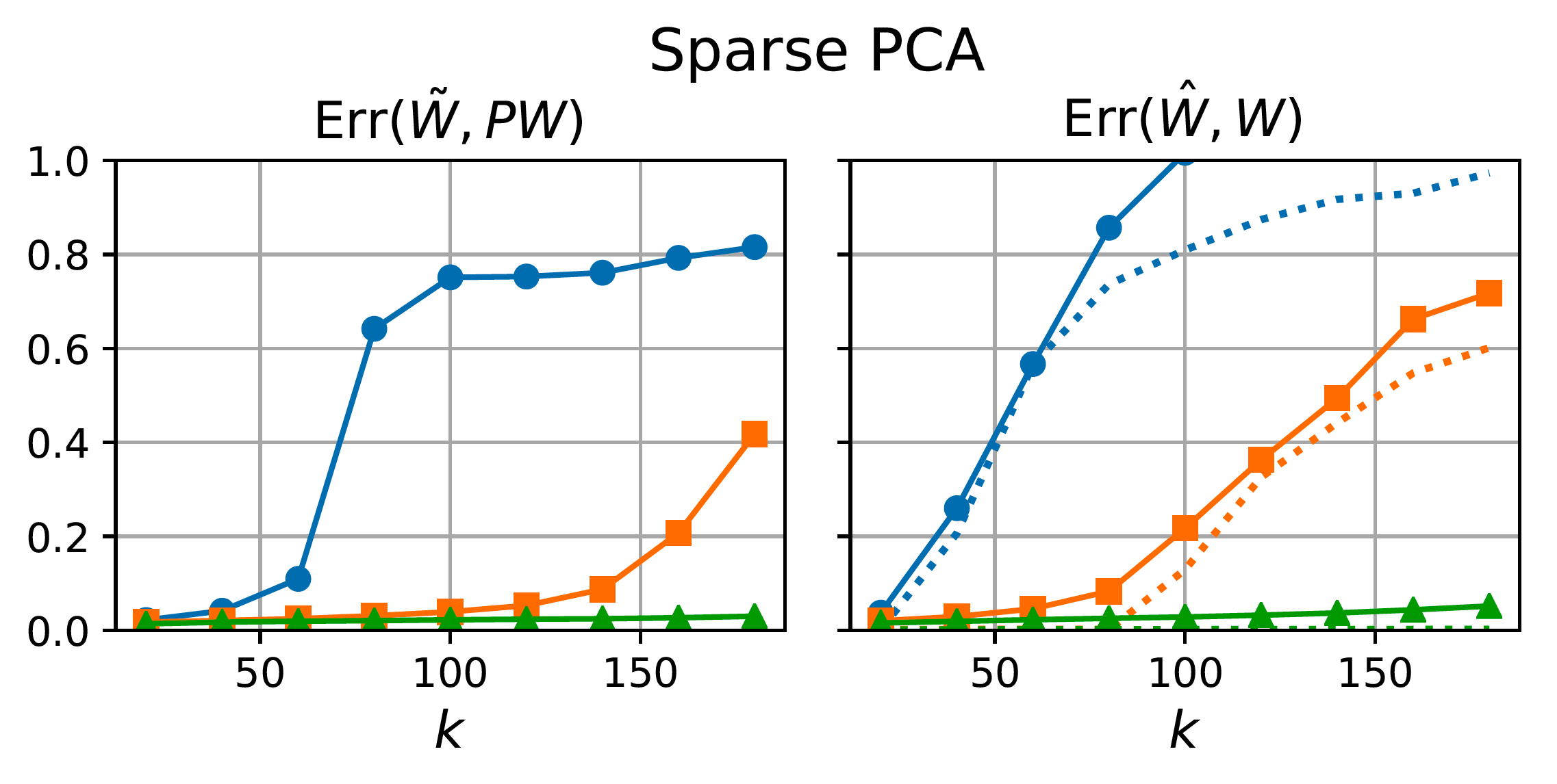
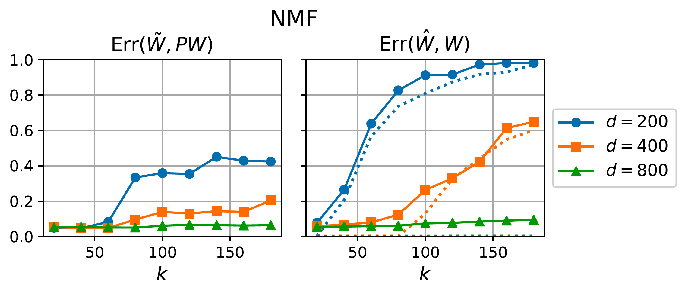
Figure 2: Approximation errors $\mathrm{Err}(X,X_{*})\coloneqq\|X-X_{*}\|_{F}/\|X_{*}\|_{F}$ for sparse PCA and NMF on synthetic data with varying column sparsity $k$ of $W$ and projection dimension $d$. The values of $d$ correspond to $10\times$, $5\times$, and $2.5\times$ compression respectively. $\mathrm{Err}(\tilde{W},PW)$ measures the distance between factors in the compressed domain: low error here is necessary for accurate sparse recovery. $\mathrm{Err}(\hat{W},W)$ measures the error after sparse recovery: the recovered factors $\hat{W}$ typically incur only slightly higher error than the oracle lower bound (dotted lines) where $PW$ is known exactly.

We provide empirical evidence that standard algorithms for sparse PCA and NMF converge in practice to the desired sparse factorization $\tilde{M}=(PW)H$—in order to achieve accurate sparse recovery in the subsequent step, it is necessary that the compressed factor $\tilde{W}$ be a good approximation of $PW$. For sparse PCA, we use alternating minimization with LARS (Zou et al., 2006), and for NMF, we use projected gradient descent (Lin, 2007). Additionally, we evaluate the quality of the factors obtained after sparse recovery by measuring the approximation error of the recovered factors $\hat{W}$ relative to the true factors $W$.

We generate synthetic data following the conditions of Theorem 1. For sparse PCA, we sample matrices $W=B\odot Y$ and $H$, where each column of $B\in\{0,1\}^{n\times r}$ has $k$ non-zero entries chosen uniformly at random, $Y_{ij}\overset{\text{iid}}{\sim}N(0,1)$, and $H_{ij}\overset{\text{iid}}{\sim}N(0,1)$. For NMF, an elementwise absolute value function is applied to the values sampled from this distribution. The noisy data matrix is $M=WH+\mathcal{E}$, where the noise term $\mathcal{E}$ is a dense random Gaussian matrix scaled such that $\|\mathcal{E}\|_{F}/\|WH\|_{F}=0.1$. We observe $\tilde{M}=PM$, where $P$ has $p=5$ non-zero entries per column (in the Appendix, we study the effect of varying $p$ on the error).

Figure 2 shows our results on synthetic data with $m=2000$, $n=2000$, and $r=10$. For small column sparsities $k$ relative to the projection dimension $d$, the estimated compressed left factors $\tilde{W}$ are good approximations to the desired solutions $PW$. Encouragingly, we find that the recovered solutions $\hat{W}=\mathcal{R}(\tilde{W})$ are typically only slightly worse in approximation error than $\mathcal{R}(PW)$, the solution recovered when the projection of $W$ is known exactly. Thus, we perform almost as well as the idealized setting where we are given the correct factorization $(PW)H$.

5.2 NMF on Gene Expression Data

Table 1: Summary of DNA microarray gene expression datasets, along with runtime (seconds) for each stage of the NMF pipeline on compressed data. Factorize-Recover runs only $r$ instances of sparse recovery, as opposed to the $m$ instances used by the alternative, Recover-Factorize.

Dataset	# Samples	# Features	Recover-Fac.			Fac.-Recover
			Recovery	NMF		NMF	Recovery
CNS tumors	266	7,129	76.1	2.7		0.6	5.4
Lung carcinomas	203	12,600	78.8	4.0		0.8	9.3
Leukemia	435	54,675	878.4	39.6		6.9	55.0

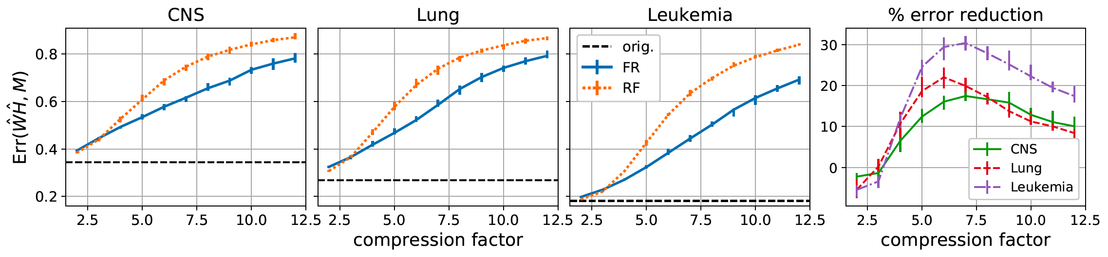
Figure 3: Normalized reconstruction errors $\|\hat{W}\hat{H}-M\|_{F}/\|M\|_{F}$ for NMF on gene expression data with varying compression factors $n/d$. FR (blue, solid) is Factorize-Recover, RF (orange, dotted) is Recover-Factorize. The horizontal dashed line is the error when $M$ is decomposed in the original space. Perhaps surprisingly, when $n/d>3$, we observe a reduction in reconstruction error when compressed data is first factorized. See the text for further discussion.

NMF is a commonly-used method for clustering gene expression data, yielding interpretable factors in practice (Gao and Church, 2005; Kim and Park, 2007). In the same domain, compressive sensing techniques have emerged as a promising approach for efficiently measuring the (sparse) expression levels of thousands of genes using compact measurement devices (Parvaresh et al., 2008; Dai et al., 2008; Cleary et al., 2017). We evaluated our proposed NMF approach on gene expression datasets targeting three disease classes: embryonal central nervous system tumors (Pomeroy et al., 2002), lung carcinomas (Bhattacharjee et al., 2001), and leukemia (Mills et al., 2009) (Table 1). Each dataset is represented as a real-valued matrix where the $i$th row denotes expression levels for the $i$th gene across each sample.

Experimental Setup.  For all datasets, we fixed rank $r=10$ following previous clustering analyses in this domain (Gao and Church, 2005; Kim and Park, 2007). For each data matrix $M\in\mathbb{R}^{n\times m}$, we simulated compressed measurements $\tilde{M}\in\mathbb{R}^{d\times m}$ by projecting the feature dimension: $\tilde{M}=PM$. We ran projected gradient descent (Lin, 2007) for 250 iterations, which was sufficient for convergence.

Computation Time.  Computation time for NMF on all 3 datasets (Table 1) is dominated by the cost of solving instances of the LP (1). As a result, Factorize-Recover achieves much lower runtime as it requires a factor of $m/r$ fewer calls to the sparse recovery procedure. While fast iterative recovery procedures such as SSMP (Berinde and Indyk, 2009) achieve faster recovery times, we found that they require approximately $2\times$ the number of measurements to achieve comparable accuracy to LP-based sparse recovery.

Reconstruction Error.  For a fixed number of measurements $d$, we observe that the Factorize-Recover procedure achieves lower approximation error than the alternative method of recovering prior to factorizing (Figure 3). While this phenomenon is perhaps counter-intuitive, it can be understood as a consequence of the sparsifying effect of NMF. Recall that for NMF, we model each column of the compressed data $\tilde{M}$ as a nonnegative linear combination of the columns of $\tilde{W}$. Due to the nonnegativity constraint on the entries of $\tilde{W}$, we expect the average sparsity of the columns of $\tilde{W}$ to be at least that of the columns of $\tilde{M}$. Therefore, if $\tilde{W}$ is a good approximation of $PW$, we should expect that the sparse recovery algorithm will recover the columns of $W$ at least as accurately as the columns of $M$, given a fixed number of measurements.

5.3 Tensor Decomposition on EEG Time Series Data

EEG readings are typically organized as a collection of time series, where each series (or channel) is a measurement of electrical activity in a region of the brain. Order-3 tensors can be derived from this data by computing short-time Fourier transforms (STFTs) for each channel, yielding a tensor where each slice is a time-frequency matrix. We experimented with tensor decomposition on a compressed tensor derived from the CHB-MIT Scalp EEG Database (Shoeb and Guttag, 2010). In the original space, this tensor has dimensions $27804\times 303\times 23$ ($\text{time}\times\text{frequency}\times\text{channel}$), corresponding to 40 hours of data (see the Appendix  for further preprocessing details). The tensor was randomly projected along the temporal axis. We then computed a rank-10 non-negative CP decomposition of this tensor using projected Orth-ALS (Sharan and Valiant, 2017).

Reconstruction Error.  At projection dimension $d=1000$, we find that Factorize-Recover achieves comparable error to Recover-Factorize (normalized Frobenius error of $0.83$ vs. $0.82$). However, RF is three orders of magnitude slower than FR on this task due to the large number of sparse recovery invocations required (once for each frequency bin/channel pair, or $303\times 23=6969$).

Factor Interpretability.  The EEG time series data was recorded from patients suffering from epileptic seizures (Shoeb and Guttag, 2010). We found that the tensor decomposition yields a factor that correlates with the onset of seizures (Figure 4). At $5\times$ compression, the recovered factor qualitatively retains the interpretability of the factor obtained by decomposing the tensor in the original space.

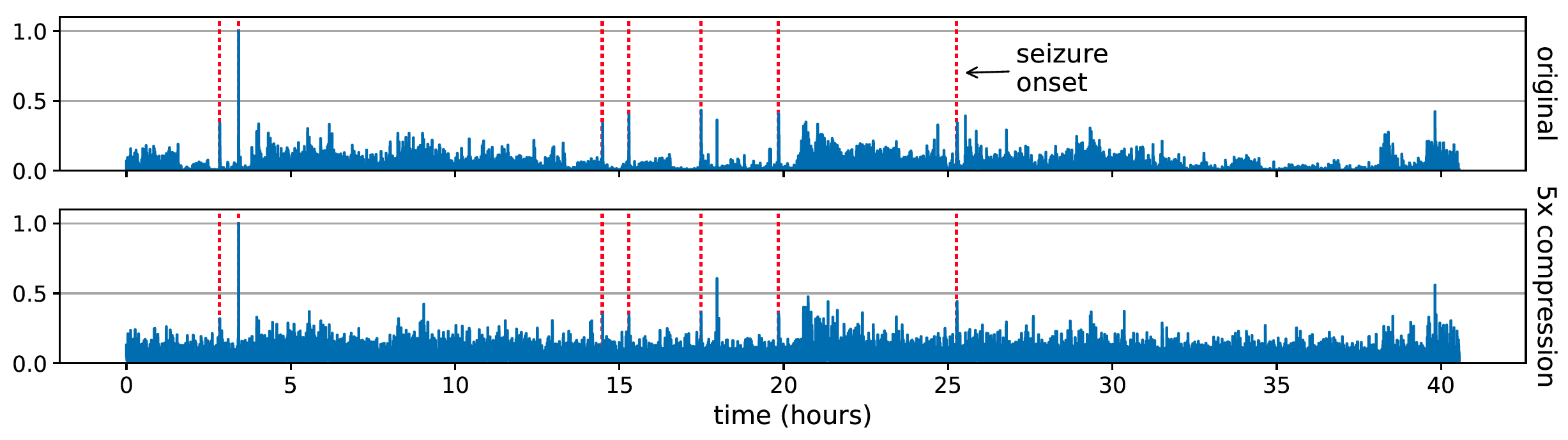
Figure 4: Visualization of a factor from the tensor decomposition of EEG data that correlates with the onset of seizures in a patient (red dotted lines). The factor recovered from a $5\times$ compressed version of the tensor (bottom) retains the peaks that are indicative of seizures.

6 Discussion and Conclusion

We briefly discuss our theoretical results on the uniqueness of sparse matrix factorizations in the context of dimensionality reduction via random projections. Such projections are known to preserve geometric properties such as pairwise distances (Kane and Nelson, 2014) and even singular vectors and singular vectors (Halko et al., 2011). Here, we showed that maximally sparse solutions to certain factorization problems are preserved by sparse binary random projections. Therefore, our results indicate that random projections can also, in a sense, preserve certain solutions of non-convex, NP-Hard problems like NMF (Vavasis, 2009).

To conclude, in this work we analyzed low-rank matrix and tensor decomposition on compressed data. Our main theoretical contribution is a novel uniqueness result for the matrix factorization case that relates sparse solutions in the original and compressed domains. We provided empirical evidence on real and synthetic data that accurate recovery can be achieved in practice. More generally, our results in this setting can be interpreted as the unsupervised analogue to previous work on supervised learning on compressed data. A promising direction for future work in this space is to examine other unsupervised learning tasks which can directly performed in the compressed domain by leveraging sparsity.

Appendix A Supplementary Experimental Results

A.1 Additional Experimental Details

Non-negative Matrix Factorization.  We optimize the following NMF objective:

$$\underset{W,H}{\mathrm{minimize}} \quad\|M-WH\|_{F}^{2}$$

subject to $$\quad W_{ij}\geq 0,H_{jk}\geq 0\quad\forall i,j,k$$

for $M\in\mathbb{R}^{n\times m}$, $W\in\mathbb{R}^{n\times r}$, $H\in\mathbb{R}^{r\times m}$. We minimize this objective with alternating non-negative least squares using the projected gradient method [Lin, 2007]. In our experiments, we initialized the entries of $W$ and $H$ using the absolute value of independent mean-zero Gaussian random variables with variance $\frac{1}{nm}\sum_{i,j}M_{ij}/r$. We use the same step size rule as in Lin [2007] with an initial step size of $1$.

Sparse PCA.  We optimize the following sparse PCA objective:

$$\underset{W,H}{\mathrm{minimize}} \quad\frac{1}{2}\|M-WH\|_{F}^{2}+\lambda\|W\|_{1}$$

subject to $$\quad\sum_{j=1}^{m}H_{ij}^{2}=1\text{ for }1\leq i\leq r.$$

The hyperparameter $\lambda\geq 0$ controls the degree of sparsity of the factor $W$. We optimize this objective via alternating minimization with LARS, using the open source SparsePCA implementation in scikit-learn 0.20.0 with its default settings. Here, the factors $W$ and $H$ are initialized deterministically using the truncated SVD of $M$.

Non-negative CP Tensor Decomposition.  We optimize the following objective:

$$\underset{A,B,C}{\mathrm{minimize}} \quad\|T-\sum_{\ell=1}^{r}A_{\ell}\otimes B_{\ell}\otimes C_{\ell}\|_{F}^{2}$$

subject to $$\quad A_{i\ell}\geq 0,B_{j\ell}\geq 0,C_{k\ell}\geq 0\quad\forall i,j,k,\ell$$

for $T\in\mathbb{R}^{n\times m_{1}\times m_{2}}$, $A\in\mathbb{R}^{n\times r}$, $B\in\mathbb{R}^{m_{1}\times r}$, $C\in\mathbb{R}^{m_{2}\times r}$. We optimize this objective using a variant of Orthogonalized Alternating Least Squares, or Orth-ALS [Sharan and Valiant, 2017] where the entries of each iterate is projected after each update such that their values are non-negative. We initialize the entries of $A$, $B$, and $C$ using the absolute value of independent standard normal random variables. For the EEG time series experiment, we use the open source MATLAB implementation of Orth-ALS, modified to incorporate the non-negativity constraint.

A.2 NMF Reconstruction Error and Projection Matrix Column Sparsity ($p$)

We investigated the trade-off between reconstruction error (as measured by normalized Frobenius loss) and the sparsity parameter $p$ of the binary random projections $P$. Recall that $P\in\{0,1\}^{d\times n}$ is a randomly sampled sparse binary matrix where $p$ distinct entries in each column are selected uniformly at random and set to 1. In Figure 5, we plot the normalized reconstruction error achieved by NMF using Factorize-Recover on the lung carcinoma gene expression dataset [Bhattacharjee et al., 2001] at a fixed compression level of 5. Since we observed that the cost of sparse recovery increases roughly linearly with $p$, we aimed to select a small value of $p$ that achieves good reconstruction accuracy. We found that the setting $p=5$ was a reasonable choice for our experiments.

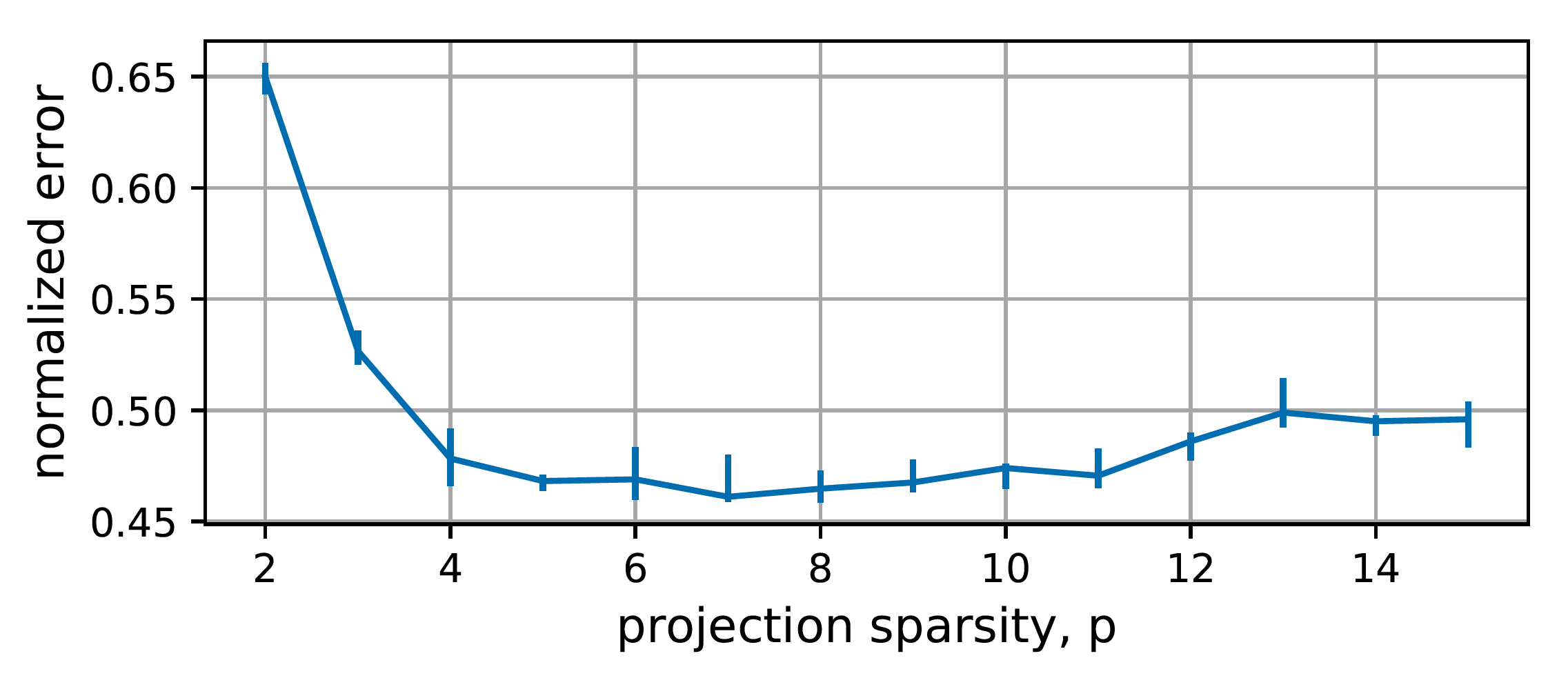
Figure 5: NMF reconstruction error vs. projection matrix column sparsity.

A.3 Preprocessing of EEG Data

Each channel is individually whitened with a mean and standard deviation estimated from segments of data known to not contain any periods of seizure. The spectrogram is computed with a Hann window of size 512 (corresponding to two seconds of data). The window overlap is set to 64. In order to capture characteristic sequences across time windows, we transform the spectrogram by concatenating groups of sequential windows, following [Shoeb and Guttag, 2010]. We concatenate groups of size three.

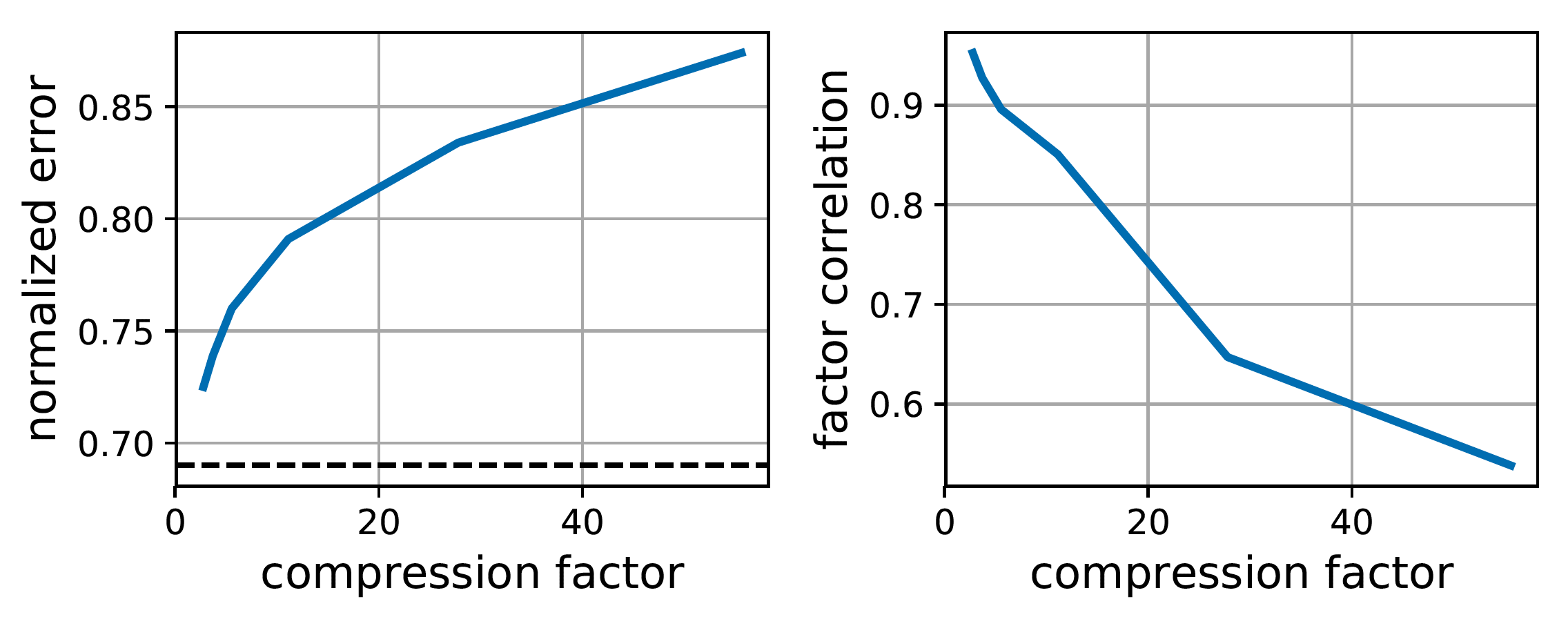
Figure 6: Accuracy of tensor decomposition on compressed EEG data. Left: Normalized reconstruction error; dashed line indicates baseline reconstruction error on original data. Right: Median Pearson correlations between recovered factors and factors computed from original data.

A.4 Tensor Decomposition of Compressed EEG Data

In Figure 6 (left), we plot the normalized Frobenius errors of the recovered factorization against the compression factor $n/d$. Due to the sparsity of the data, we can achieve over $10\times$ compression for the cost of a $10\%$ increase in reconstruction error relative to the baseline decomposition on the uncompressed data, or approximately $28\times$ compression for a $15\%$ increase. Recover-Factorize (RF) achieves slightly lower error at a given projection dimension: at $28\times$ compression ($d=1000$), RF achieves a normalized error of $0.819$ vs. $0.834$ for Factorize-Recover. However, RF is three orders of magnitude slower than Factorize-Recover on this dataset due to the large number of calls required to the sparse recovery algorithm (once for each frequency bin/channel pair, or $303\times 23=6969$) to fully recover the data tensor. Due to the computational expense of recovering the full collection of compressed time series, we did not compare RF to FR over the full range of compression factors plotted in the figure for FR.

Figure 6 (right) shows the median Pearson correlations between the columns of the recovered temporal factor and those computed on the original, uncompressed data (paired via maximum bipartite matching). At up to $10\times$ compression, the recovered temporal factors match the temporal factors obtained by factorization on the uncompressed data with a median correlation above $0.85$. Thus, compressed tensor factorization is able to successfully recover an approximation to the factorization of the uncompressed tensor.

Appendix B Proof of Theorem 1: Uniqueness for NMF

We follow the outline from the proof sketch. Recall that our goal will be to prove that the columns of $\tilde{W}$ are the sparsest vectors in the column space of $\tilde{W}$. For readability proofs of some auxiliary lemmas appears later in Section B.1

As mentioned in the proof sketch, the first step is part (a)—showing that if we take any subset $S$ of the columns of $\tilde{W}$, then the number of rows which have non-zero entries in at least one of the columns in $S$ is large. Lemma 1 shows that the number of rows which are have at least one zero entry in a subset $S$ of the columns of $W$ columns proportionately with the size of $S$. The proof proceeds by showing that choosing $B$ such that each column has $k$ randomly chosen non-zero entries ensures expansion for $B$ with high probability, and we have already ensured expansion for $P$ with high probability.

Lemma 1.

For any subset $S$ of the columns of $\tilde{W}$, define $N(S)$ to be the subset of the rows of $\tilde{W}$ which have a non-zero entry in at least one of the columns in $S$. Then for every subset $S$ of columns of $\tilde{W}$, $|N(S)|\geq\min\{16|S|kp/25,d/200\}$ with failure probability $re^{-\beta k}/n+(1/n^{5})$.

We now prove the second part of the argument—that any linear combination of columns in $S$ cannot have much fewer non-zero entries than $N(S)$, as the probability that many of the non-zero entries get canceled is zero. Lemma 2 is the key to showing this. Define a vector $x$ as fully dense if all its entries are non-zero.

Lemma 2.

For any subset $S$ of the columns of $\tilde{W}$, let $U$ be the submatrix of $\tilde{W}$ corresponding to the $S$ columns and $N(S)$ rows. Then with probability one, every subset of the rows of $U$ of size at least $|S|p$ does not have any fully dense vector in its right null space.

Proof.

Without loss of generality, assume that $S$ corresponds to the first $|S|$ columns of $\tilde{W}$, and $N(S)$ corresponds to the first $|N(S)|$ rows of $\tilde{W}$. We will partition the rows of $U$ into $t$ groups $\{\mathcal{G}_{1},\dots,\mathcal{G}_{t}\}$. Each group will have size at most $p$. To select the first group, we choose any entry $y_{1}$ of $Y$ which appears in the first row of $U$. For example, if the first column of $W$ has a one in its first row, and $P(1,1)=1$, then the random variable $Y_{1,1}$ appears in the first row of $U$. Say we choose $y_{1}=Y_{1,1}$. We then choose $\mathcal{G}_{1}$ to be the set of all rows where $y_{1}$ appears. We then remove the set of rows $\mathcal{G}_{1}$ from $U$. To select the second group, we pick any one of the remaining rows, and choose any entry $y_{2}$ of $Y$ which appears in that row of $U$. $\mathcal{G}_{2}$ is the set of all rows where $y_{2}$ appears. We repeat this procedure to obtain $t$ groups, each of which will have size at most $p$ as every variable appears in $p$ columns. Hence any subset of rows of size at least $|S|p$ must correspond to at least $|S|$ groups.

Let $\mathcal{N}_{j}$ be the right null space of the first $j$ groups of rows. We define $\mathcal{N}_{0}=\mathbb{R}^{|S|}$. We will now show that either $\text{rank}(\mathcal{N}_{i})=|S|-i$ or $\mathcal{N}_{i}$ does not contain a fully dense vector. We prove this by induction. Consider the $j$th step, at which we have $j$ groups $\{\mathcal{G}_{1},\dots,\mathcal{G}_{j}\}$. By the induction hypothesis, either $\mathcal{N}_{j}$ does not contain any fully dense vector, or $\text{rank}(\mathcal{N}_{j})=|S|-j$. If $\mathcal{N}_{j}$ does not contain any fully dense vector, then we are done as this implies that $\mathcal{N}_{j+1}$ also does not contain any fully dense vector. Assume that $\mathcal{N}_{j}$ contains a fully dense vector $x$. Choose any row $U_{c}$ which has not been already been assigned to one of the sets. By the following elementary proposition, the probability that $x$ is orthogonal to $U_{c}$ is zero. We provide a simple proof in Section B.1.

Lemma 3.

Let $v=(v_{1},\dots,v_{n})\in\mathbb{R}^{n}$ be a vector of $n$ independent random variables drawn from some continuous distribution. For any subset $S\subseteq\{1,\dots,n\}$, let $v(S)\in\mathbb{R}^{|S|}$ refer to the subset of $v$ corresponding to the indices in $S$. Consider $t$ such subsets $S_{1},\dots,S_{t}$. Let each set $S_{i}$ defines some linear relation $\alpha_{S_{i}}^{T}v(S_{i})=0$, for some $\alpha_{S_{i}}\in\mathbb{R}^{|S_{i}|}$ where $\|\alpha_{S_{i}}\|=1$ and each entry of the vector $\alpha_{S_{i}}$ is non-zero on the variables in the set $S_{i}$. Assume that the variable $v_{i}$ appears in the set $S_{i}$. Then the probability distribution of the set of variables $\{v_{t+1},\dots,v_{n}\}$ conditioned on the linear relations defined by $S_{1},\dots,S_{t}$ is still continuous, and hence any linear combination of the set of variables $\{v_{t+1},\dots,v_{n}\}$ has zero probability of being zero.

If $\mathcal{N}_{j}$ contains a fully dense vector, then with probability one, $\text{rank}(\mathcal{N}_{j+1})=\text{rank}(\mathcal{N}_{j})-1=n-j-1$. This proves the induction argument. Therefore, with probability one, for any $t\geq|S|$, either $\text{rank}(\mathcal{N}_{t})=0$ or $\mathcal{N}_{t}$ does not contain a fully dense vector and Lemma 2 follows. ∎

We now complete the proof of Theorem 1. Note that the columns of $\tilde{W}$ have at most $kp$ non-zero entries, as each column of $P$ has $p$-sparse. Consider any set $S$ of columns of $\tilde{W}$. Consider any linear combination $v\in\mathbb{R}^{d}$ of the set $S$ columns, such that all the combination weights $x\in\mathbb{R}^{|S|}$ are non-zero. By Lemma 1, $|N(S)|\geq\min\{16|S|kp/25,d/200\}$ with failure probability $re^{-\beta k}/n+(1/n^{5})$. We claim that $v$ has more than $|N(S)|-|S|p$ non zero entries. We prove by contradiction. Assume that $v$ has $|N(S)|-|S|$ or fewer non zero entries. Consider the submatrix $U$ of $\tilde{W}$ corresponding to the $S$ columns and $N(S)$ rows. If $v$ has $|N(S)|-|S|p$ or fewer non zero entries, then there must be a subset $S^{\prime}$ of the $|N(S)|$ rows of $U$ with $|S^{\prime}|=|S|p$, such that each of the rows in $S^{\prime}$ has at least one non-zero entry, and the fully dense vector $x$ lies in the right null space of $S^{\prime}$. But by Lemma 2, the probability of this happening is zero. Hence $v$ has more than $|N(S)|-|S|p$ non zero entries. Lemma 4 obtains a lower bound on $|N(S)|-|S|p$ using simple algebra.

Lemma 4.

$|N(S)|-|S|p\geq 6kp/5$ for $|S|>1$ for $d\geq 400p(r+k)$.

Hence any linear combination of more than one column of $\tilde{W}$ has at least $6kp/5$ non-zero entries with failure probability $re^{-\beta k}/n$. Hence the columns of $\tilde{W}$ are the sparsest vectors in the column space of $\tilde{W}$ with failure probability $re^{-\beta k}/n+(1/n^{5})$.

B.1 Additional Proofs for Uniqueness of NMF

Lemma 5.

If $H$ is full row rank, then the column spaces of $\tilde{W}$ and ${W}^{\prime}$ are equal.

Proof.

We will first show that the column space of $\tilde{M}$ equals the column space of $\tilde{W}$. Note that the column space of $\tilde{M}$ is a subspace of the column space of $\tilde{W}$. As $H$ is full row rank, the rank of the column space of $\tilde{M}$ equals the rank of the column space of $\tilde{W}$. Therefore, the column space of $\tilde{M}$ equals the column space of $\tilde{W}$.

By the same argument, for any alternative factorization $\tilde{M}=W^{\prime}H^{\prime}$, the column space of $W^{\prime}$ must equal the column space of $\tilde{M}$—which equals the column space of $\tilde{W}$. As the column space of $W^{\prime}$ equals the column space of $\tilde{W}$, therefore $W^{\prime}$ must lie in the column space of $\tilde{W}$. ∎

See 1

Proof.

We first show a similar property for the columns of $W$, and will then extend it to the columns of $\tilde{W}=PW$. We claim that for every subset of $S$ columns of $W$, $|N(S)|\geq\min\{4|S|k/5,n/200\}$ with failure probability $re^{-\beta k}/n$.

To verify, consider a bipartite graph $T$ with $r$ nodes on the left part $U_{1}$ corresponding to the $r$ columns of $W$, and $n$ nodes on the right part $V$ corresponding to the $n$ rows or indices of each factor. The $i$th node in $U_{1}$ has an edge to $k$ nodes in $V$ corresponding to the non-zero indices of the $i$th column of $W$. Note that $|N(S)|$ is the neighborhood of the set of nodes $S$ in $G$. From Part 1 of Lemma 6, the graph $G$ is a $(\gamma_{1}r,4/5)$ expander with failure probability $re^{-\beta k}/n$ for $\gamma_{1}=n/(rke^{5})$ and a fixed constant $\beta>0$.

Lemma 6.

Randomly choose a bipartite graph $G$ with $n_{1}$ vertices on the left part $U$ and $n_{2}$ vertices on the right part $V$ such that every vertex in $U$ has degree $D$. Then,

1. For every $n_{1},n_{2},n_{1}<n_{2}$, $G$ is a $(\gamma n_{1},4/5)$ expander for $D\geq c$ for some fixed constant $c$ and $\gamma n_{1}=\frac{n_{2}}{De^{5}}$ except with probability $n_{1}e^{-\beta D}/n_{2}$ for a fixed constant $\beta>0$.

2. For every $n_{1},n_{2},n_{2}<n_{1}$, $G$ is a $(\gamma n_{1},4/5)$ expander for $D\geq c\log n_{1}$ for some fixed constant $c$ and $\gamma n_{1}=\frac{n_{2}}{De^{5}}$ except with probability $(1/n_{1})^{5}$.

As $G$ is a $(\gamma_{1}r,4/5)$ expander, every set of $|S|\leq\gamma_{1}r$ nodes has at least $4|S|k/5$ neighbors. A set of size $|S|>\gamma_{1}r$ nodes, must include a subset of size $\gamma_{1}r$ which has $4n/(5e^{5})\geq n/200$ neighbours, and hence every set of size $|S|>\gamma_{1}r$ has at least $n/200$ neighbors. Therefore, for every subset of $S$ columns, $|N(S)|\geq\min\{4|S|k/5,n/200\}$ with failure probability $re^{-\beta k}/n$.

We will now extend the proof to show the necessary property for $\tilde{W}$. After the projection step, the $n$ indices are projected to $d$ dimensions, and the projection matrix is a $(\gamma_{2}n,4/5)$ expander with $\gamma_{2}=d/(nke^{5})$. We can now consider a tripartite graph, by adding a third set $U_{2}$ with $d$ nodes. We add an edge from a node $i$ in $V$ to node $j$ in $U_{2}$ if $P(j,i)=1$. For any subset $S$ of columns of $\tilde{W}$, $N(S)$ are the set of nodes in $U_{2}$ which are reachable from the nodes $S$ in $U_{1}$.

With failure probability $(1/n^{5})$, the projection matrix $P$ is a $(\gamma_{2}n,4/5)$ expander with $\gamma_{2}=d/(npe^{5})$. Therefore every subset of size $t$ in $V$ has at least $\min\{4tp/5,d/200\}$ neighbors in $W$. By combining this argument with the fact that every set of $S$ nodes in $U$, has at least $\min\{4|S|k/5,n/200\}$ neighbors with failure probability $re^{-\beta k}/n$, it follows that for every subset of $S$ columns of $\tilde{W}$, $|N(S)|\geq\min\{16|S|kp/25,d/200\}$ with failure probability $re^{-\beta k}/n+(1/n^{5})$. ∎

See 3

Proof.

We prove by induction. For the base case, note that without any linear constraints, the set of $n$ random variables $\{v_{1},\dots,v_{n}\}$ is continuous by definition. Consider the $j$th step, when linear constraints defined by the sets $S_{1},\dots,S_{j}$ have been imposed on the variables. We claim that the distribution of the set of random variables $\{v_{j+1},\dots,v_{n}\}$ is continuous after imposition of the constraints $S_{1},\dots,S_{j}$. By the induction hypothesis, the distribution of the set of random variables $\{v_{j},\dots,v_{n}\}$ is continuous after imposition of the constraints $S_{1},\dots,S_{j-1}$. Suppose that the linear constraint $\alpha_{S_{j}}$ is satisfied for some assignment $(t_{j},\dots,t_{n})$ to the random variables $\{v_{j},\dots,v_{n}\}$ which appear in the constraint $S_{j}$. As the distribution of the variables $\{v_{j},\dots,v_{n}\}$ is continuous by our induction hypothesis, there exists some $\epsilon>0$ such that the pdf of the variables $v_{i}$ for $j\leq i\leq n$ is non-zero in the interval $[t_{i}-\epsilon,t_{i}+\epsilon]$. Let $\delta=|\alpha_{S_{i}}(j)|$ be the absolute value of the linear coefficients of the variable $v_{j}$ in $\alpha_{S_{i}}$. For any choice of $v_{i},j+1\leq i\leq n$ in the interval $[t_{i}-\delta\epsilon/\sqrt{n},t_{i}+\delta\epsilon/\sqrt{n}]$, the linear constraint $\alpha_{S_{i}}$ can be satisfied by some choice of the variable $v_{j}$ in $[t_{j}-\epsilon,t_{j}+\epsilon]$. Hence the probability distribution of the set of variables $\{v_{j+1},\dots,v_{n}\}$ is still continuous after adding the constraint $S_{j}$, which proves the induction step.

∎

See 4

Proof.

For $2\leq|S|\leq d/(128kp)$,

$$|N(S)|-|S|p \geq(16kp/25)|S|-p|S|=30kp/25+kp(16|S|-30)/25-p|S|$$

$$\geq 6kp/5+p\Big{(}k(16|S|-30)-|S|\Big{)}$$

For $|S|\geq 2$ and $k\geq 2$, $k(16|S|-30)-|S|\geq 0$, hence $|N(S)|-|S|p\geq 6kp/5$ for $2\leq|S|\leq d/(128kp)$. For $|S|>d/(128kp)$, $|N(S)|\geq d/200$. Therefore, $|N(S)|-|S|p\geq d/200-rp\geq 2kp$ for $d\geq 400p(r+k)$. ∎

See 6

Proof.

Consider any subset $S\subset U$ with $|S|\leq\gamma n_{1}$. Let $\mathbb{P}(N(S)\subseteq M)$ denote the probability of the event that the neighborhood of $S$ is entirely contained in $M\subset V$. $\mathbb{P}(N(S)\subseteq M)\leq\Big{(}\frac{|M|}{n_{2}}\Big{)}^{D|S|}$. We will upper bound the probability of $G$ not being an expander by upper-bounding the probability of each subset $S\subset U$ with $|S|\leq\gamma n_{1}$ not expanding. Let $\mathbb{P}(\bar{S})$ denote the probability of the neighborhood of $S$ being entirely contained in a subset $M\subset V$ with $M<{\alpha}|S|D$. By a union bound,

$$\mathbb{P}(G\text{ is not a $(\gamma n_{1},\alpha)$ expander}) \leq\sum_{\begin{subarray}{c}S\subset U\\ |S|\leq\gamma n_{1}\end{subarray}}\mathbb{P}(\bar{S})$$

$$\leq\sum_{\begin{subarray}{c}S\subset U\\ |S|\leq\gamma n_{1}\end{subarray}}\sum_{\begin{subarray}{c}M\subset V\\ M={\alpha}|S|D\end{subarray}}\mathbb{P}(N(S)\subseteq M)$$

$$\leq\sum_{s=1}^{\gamma n_{1}}\sum_{\begin{subarray}{c}S\subset U\\ |S|=s\end{subarray}}\sum_{\begin{subarray}{c}M\subset V\\ M={\alpha}|S|D\end{subarray}}\Big{(}\frac{{\alpha}|S|D}{n_{2}}\Big{)}^{D|S|}$$

$$\leq\sum_{s=1}^{\gamma n_{1}}{n_{1}\choose s}{n_{2}\choose{\alpha}Ds}\Big{(}\frac{{\alpha}Ds}{n_{2}}\Big{)}^{Ds}$$

Using the bound ${n\choose k}\leq(ne/k)^{k}$, we can write,

$$\mathbb{P}(G\text{ is not a $(\gamma n_{1},\alpha)$ expander}) \leq\sum_{s=1}^{\gamma n_{1}}\Big{(}\frac{n_{1}e}{s}\Big{)}^{{\alpha}s}\Big{(}\frac{n_{2}e}{{\alpha}Ds}\Big{)}^{{\alpha}Ds}\Big{(}\frac{{\alpha}Ds}{n_{2}}\Big{)}^{Ds}$$

$$\leq\sum_{s=1}^{\gamma n_{1}}\Bigg{[}\Big{(}\frac{n_{1}e}{s}\Big{)}^{{\alpha}}\Big{(}\frac{n_{2}e}{{\alpha}Ds}\Big{)}^{{\alpha}D}\Big{(}\frac{{\alpha}Ds}{n_{2}}\Big{)}^{D}\Bigg{]}^{s}\leq\sum_{s=1}^{\gamma n_{1}}x_{s}^{s}$$

where $x_{s}=\Big{(}\frac{n_{1}e}{s}\Big{)}\Big{(}\frac{n_{2}e}{{\alpha}Ds}\Big{)}^{{\alpha}D}\Big{(}\frac{{\alpha}Ds}{n_{2}}\Big{)}^{D}$. $x_{s}$ can be bounded as follows—

$$x_{s} =\Big{(}\frac{n_{1}e}{s}\Big{)}\Big{(}\frac{{\alpha}Dse^{1/{(1-\alpha)}}}{n_{2}}\Big{)}^{{(1-\alpha)}D}$$

$$\leq\Big{(}\frac{e}{\gamma}\Big{)}\Big{(}\frac{{\alpha}D\gamma n_{1}e^{1/(1-\alpha)}}{n_{2}}\Big{)}^{{(1-\alpha)}D}$$

$$\leq\Big{(}\frac{n_{1}e^{1+1/(1-\alpha)}}{n_{2}}\Big{)}D{\alpha}^{{(1-\alpha)}D}$$

$$\leq\Big{(}\frac{n_{1}e^{6}}{n_{2}}\Big{)}De^{-D/25}=x$$

where in the last step we set $\alpha=4/5$. Hence we can upper bound the probability of $G$ not being an expander as follows—

$$\mathbb{P}(G\text{ is not a $(\gamma n_{1},\alpha)$ expander})\leq\sum_{s=1}^{\infty}x^{s}\leq\frac{x}{1-x}$$

The two parts of Lemma 6 follow by plugging in the respective values for $n_{1},n_{2}$ and $D$. ∎

Appendix C Recovery Guarantees for Compressed Tensor Factorization using ALS-based Methods

We can prove a stronger result for symmetric, incoherent tensors and guarantee accurate recovery in the compressed space using the tensor power method. The tensor power method is the tensor analog of the matrix power method for finding eigenvectors. It is equivalent to finding a rank 1 factorization using the Alternating Least Squares (ALS) algorithm. Incoherent tensors are tensors for which the factors have small inner products with other. We define the incoherence $\mu=\max_{i\neq j}\{|A_{i}^{T}A_{j}|\}$. Our guarantees for tensor decomposition follow from the analysis of the tensor power method by Sharan and Valiant [2017]. Proposition 2 shows guarantees for recovering one of the true factors, multiple random initializations can then be used for the tensor power method to recover back all the factors (see Anandkumar et al. [2014]).

Proposition 2.

Consider a $n$-dimensional rank $r$ tensor $T=\sum_{i=1}^{r}w_{i}A_{i}\otimes A_{i}\otimes A_{i}$. Let $c_{\max}=\max_{i\neq j}|A_{i}^{T}A_{j}|$ be the incoherence between the true factors and $\gamma=\frac{w_{\max}}{w_{\min}}$ be the ratio of the largest and smallest weight. Assume $\gamma$ is a constant and $\mu\leq o(r^{-2})$. Consider a projection matrix $P\in\{0,\pm 1\}^{n\times d}$ where every row has exactly $p$ non-zero entries, chosen uniformly and independently at random and the non-zero entries have uniformly and independently distributed signs. We take $d=O(r^{4}\log r)$ and $p=O(r^{2}\log r)$. Let $\tilde{A}=AP$ and $\tilde{T}$ be the $d$ dimensional projection of $T$, hence $\tilde{T}=\sum_{i=1}^{k}w_{i}\tilde{A}_{i}\otimes\tilde{A}_{i}\otimes\tilde{A}_{i}$. Then for the projected tensor decomposition problem, if the initialization $x_{0}\in\mathbb{R}^{d}$ is chosen uniformly at random from the unit sphere, then with high probability the tensor power method converges to one of the true factors of $\tilde{T}$ (say the first factor $\tilde{A}_{1}$) in $O(r(\log r+\log\log d))$ steps, and the estimate $\tilde{A}^{\prime}$ satisfies $\|\tilde{A}_{1}-\tilde{A}_{1}^{\prime}\|_{2}^{2}\leq O(r\max\{\mu^{2},1/d^{2}\})$.

Proof.

Our proof relies on Theorem 3 of Sharan and Valiant [2017] and sparse Johnson Lindenstrauss transforms due to Kane and Nelson [2014]. To show Claim 2 we need to ensure that the incoherence parameter in the projected space is small. We use the Johnson Lindenstrauss property of our projection matrix to ensure this. A matrix $M$ is regarded as a Johnson Lindenstrauss matrix if it preserves the norm of a randomly chosen unit vector $x$ up to a factor of $(1\pm\epsilon)$, with failure probabilty $\delta$:

$$\mathbb{P}_{x}[(1-\epsilon)<\|Mx\|_{2}^{2}<(1+\epsilon)]>1-\delta.$$

We use the results of Kane and Nelson [2014] who show that with high probability a matrix $P\in\{0,\pm 1\}^{n\times d}$ where every row has $p$ non-zero entries, chosen uniformly and independently at random and the non-zero entries have uniformly and independently distributed signs, preserves pairwise distances to within a factor $\epsilon$ for $d=O(\epsilon^{-2}\log(1/\delta))$ and $p=\Theta(\epsilon^{-1}\log(1/\delta))$.

It is easy to verify that inner-products are preserved to within an additive error $\epsilon$ if the pairwise distances are preserved to within a factors of $(1\pm\epsilon)$. By choosing $\delta=1/r^{3}$ and doing a union bound over all the $r^{2}$ pairs of factors, the factors are $(\mu\pm\epsilon)$ incoherent in the projected space with high probability if they were $\mu$ incoherent in the original space. Setting $\epsilon=r^{-2}\log^{-1}r$ ensures that $\mu+\epsilon=o(r^{-2})$. Claim 2 now again follows from Theorem 3 of Sharan and Valiant [2017]. ∎

References

- Donoho [2006] David L Donoho. Compressed sensing. IEEE Transactions on information theory, 52(4):1289–1306, 2006.
- Candès and Wakin [2008] Emmanuel J Candès and Michael B Wakin. An introduction to compressive sampling. IEEE Signal Processing Magazine, 2008.
- Haupt et al. [2008] Jarvis Haupt, Waheed U Bajwa, Michael Rabbat, and Robert Nowak. Compressed sensing for networked data. IEEE Signal Processing Magazine, 2008.
- Abdulghani et al. [2012] Amir M Abdulghani, Alexander J Casson, and Esther Rodriguez-Villegas. Compressive sensing scalp EEG signals: implementations and practical performance. Medical & Biological Engineering & Computing, 2012.
- Duarte et al. [2008] Marco F Duarte, Mark A Davenport, Dharmpal Takhar, Jason N Laska, Ting Sun, Kevin F Kelly, and Richard G Baraniuk. Single-pixel imaging via compressive sampling. IEEE Signal Processing Magazine, 25(2):83–91, 2008.
- Cormode et al. [2012] Graham Cormode, Minos Garofalakis, Peter J Haas, and Chris Jermaine. Synopses for massive data: Samples, histograms, wavelets, sketches. Foundations and Trends in Databases, 4(1–3):1–294, 2012.
- Calderbank et al. [2009] Robert Calderbank, Sina Jafarpour, and Robert Schapire. Compressed learning: Universal sparse dimensionality reduction and learning in the measurement domain. preprint, 2009.
- Durrant and Kabán [2010] Robert J Durrant and Ata Kabán. Compressed Fisher linear discriminant analysis: Classification of randomly projected data. In KDD, 2010.
- Fowler [2009] James E Fowler. Compressive-projection principal component analysis. IEEE Transactions on Image Processing, 18(10):2230–2242, 2009.
- Zhou and Tao [2011] Tianyi Zhou and Dacheng Tao. Godec: Randomized low-rank & sparse matrix decomposition in noisy case. In International conference on machine learning. Omnipress, 2011.
- Ha and Barber [2015] Wooseok Ha and Rina Foygel Barber. Robust PCA with compressed data. In Advances in Neural Information Processing Systems, pages 1936–1944, 2015.
- Zhou et al. [2009] Shuheng Zhou, John Lafferty, and Larry Wasserman. Compressed and privacy-sensitive sparse regression. IEEE Transactions on Information Theory, 55(2):846–866, 2009.
- Maillard and Munos [2009] Odalric Maillard and Rémi Munos. Compressed least-squares regression. In Advances in Neural Information Processing Systems, pages 1213–1221, 2009.
- Kabán [2014] Ata Kabán. New bounds on compressive linear least squares regression. In Artificial Intelligence and Statistics, pages 448–456, 2014.
- Gao and Church [2005] Yuan Gao and George Church. Improving molecular cancer class discovery through sparse non-negative matrix factorization. Bioinformatics, 2005.
- Parvaresh et al. [2008] Farzad Parvaresh, Haris Vikalo, Sidhant Misra, and Babak Hassibi. Recovering sparse signals using sparse measurement matrices in compressed DNA microarrays. IEEE Journal of Selected Topics in Signal Processing, 2008.
- Amini et al. [2009] Massih Amini, Nicolas Usunier, and Cyril Goutte. Learning from multiple partially observed views-an application to multilingual text categorization. In Advances in Neural Information Processing Systems, 2009.
- Deshpande and Montanari [2014] Yash Deshpande and Andrea Montanari. Sparse PCA via covariance thresholding. In Advances in Neural Information Processing Systems, pages 334–342, 2014.
- Papailiopoulos et al. [2013] Dimitris Papailiopoulos, Alexandros Dimakis, and Stavros Korokythakis. Sparse pca through low-rank approximations. In International Conference on Machine Learning, pages 747–755, 2013.
- Arora et al. [2012] Sanjeev Arora, Rong Ge, and Ankur Moitra. Learning topic models–going beyond SVD. In Foundations of Computer Science (FOCS), 2012 IEEE 53rd Annual Symposium on, pages 1–10. IEEE, 2012.
- Vavasis [2009] Stephen A Vavasis. On the complexity of nonnegative matrix factorization. SIAM Journal on Optimization, 20(3):1364–1377, 2009.
- Lee and Seung [1999] Daniel D Lee and H Sebastian Seung. Learning the parts of objects by non-negative matrix factorization. Nature, 1999.
- Hoyer [2004] Patrik O Hoyer. Non-negative matrix factorization with sparseness constraints. JMLR, 2004.
- Li et al. [2001] Stan Z Li, Xin Wen Hou, Hong Jiang Zhang, and Qian Sheng Cheng. Learning spatially localized, parts-based representation. In Computer Vision and Pattern Recognition, 2001. CVPR 2001. Proceedings of the 2001 IEEE Computer Society Conference on, volume 1, pages I–I. IEEE, 2001.
- Kim and Park [2008] Jingu Kim and Haesun Park. Sparse nonnegative matrix factorization for clustering. Technical report, Georgia Institute of Technology, 2008.
- Peharz and Pernkopf [2012] Robert Peharz and Franz Pernkopf. Sparse nonnegative matrix factorization with l0-constraints. Neurocomputing, 80:38–46, 2012.
- Kolda and Bader [2009] Tamara G Kolda and Brett W Bader. Tensor decompositions and applications. SIAM Review, 2009.
- Halko et al. [2011] Nathan Halko, Per-Gunnar Martinsson, and Joel A Tropp. Finding structure with randomness: Probabilistic algorithms for constructing approximate matrix decompositions. SIAM review, 53(2):217–288, 2011.
- Clarkson and Woodruff [2013] Kenneth L Clarkson and David P Woodruff. Low rank approximation and regression in input sparsity time. In Proceedings of the forty-fifth annual ACM symposium on Theory of computing. ACM, 2013.
- Wang and Li [2010] Fei Wang and Ping Li. Efficient nonnegative matrix factorization with random projections. In Proceedings of the 2010 SIAM International Conference on Data Mining. SIAM, 2010.
- Tepper and Sapiro [2016] Mariano Tepper and Guillermo Sapiro. Compressed nonnegative matrix factorization is fast and accurate. IEEE Transactions on Signal Processing, 64(9):2269–2283, 2016.
- Battaglino et al. [2017] Casey Battaglino, Grey Ballard, and Tamara G Kolda. A practical randomized CP tensor decomposition. arXiv preprint arXiv:1701.06600, 2017.
- Hsu et al. [2009] Daniel J Hsu, Sham M Kakade, John Langford, and Tong Zhang. Multi-label prediction via compressed sensing. In Advances in neural information processing systems, pages 772–780, 2009.
- Yoo and Choi [2011] Jiho Yoo and Seungjin Choi. Matrix co-factorization on compressed sensing. In IJCAI, volume 22, page 1595, 2011.
- Duarte and Baraniuk [2012] Marco F Duarte and Richard G Baraniuk. Kronecker compressive sensing. IEEE Transactions on Image Processing, 2012.
- Caiafa and Cichocki [2013] Cesar F Caiafa and Andrzej Cichocki. Multidimensional compressed sensing and their applications. Wiley Interdisciplinary Reviews: Data Mining and Knowledge Discovery, 2013.
- Caiafa and Cichocki [2015] Cesar F Caiafa and Andrzej Cichocki. Stable, robust, and super fast reconstruction of tensors using multi-way projections. IEEE Transactions on Signal Processing, 2015.
- Sidiropoulos and Kyrillidis [2012] Nicholas D Sidiropoulos and Anastasios Kyrillidis. Multi-way compressed sensing for sparse low-rank tensors. IEEE Signal Processing Letters, 2012.
- Spielman et al. [2012] Daniel A Spielman, Huan Wang, and John Wright. Exact recovery of sparsely-used dictionaries. In Conference on Learning Theory, pages 37–1, 2012.
- Candes and Tao [2006] Emmanuel J Candes and Terence Tao. Near-optimal signal recovery from random projections: Universal encoding strategies? IEEE Transactions on Information Theory, 2006.
- Candes [2008] Emmanuel J Candes. The restricted isometry property and its implications for compressed sensing. Comptes Rendus Mathematique, 2008.
- Berinde et al. [2008a] Radu Berinde, Piotr Indyk, and Milan Ruzic. Practical near-optimal sparse recovery in the l1 norm. In Allerton, 2008a.
- Indyk and Ruzic [2008] Piotr Indyk and Milan Ruzic. Near-optimal sparse recovery in the l1 norm. In FOCS, 2008.
- Berinde and Indyk [2009] Radu Berinde and Piotr Indyk. Sequential sparse matching pursuit. In Allerton Conference on Communication, Control, and Computing, 2009.
- Berinde et al. [2008b] Radu Berinde, Anna C Gilbert, Piotr Indyk, Howard Karloff, and Martin J Strauss. Combining geometry and combinatorics: A unified approach to sparse signal recovery. In Allerton Conference on Communication, Control, and Computing, 2008b.
- Indyk et al. [2010] Piotr Indyk, Hung Q Ngo, and Atri Rudra. Efficiently decodable non-adaptive group testing. In Proceedings of the twenty-first annual ACM-SIAM symposium on Discrete Algorithms, 2010.
- Hoory et al. [2006] Shlomo Hoory, Nathan Linial, and Avi Wigderson. Expander graphs and their applications. Bulletin of the American Mathematical Society, 2006.
- Vadhan et al. [2012] Salil P Vadhan et al. Pseudorandomness. Foundations and Trends® in Theoretical Computer Science, 7(1–3):1–336, 2012.
- Kruskal [1977] Joseph B Kruskal. Three-way arrays: Rank and uniqueness of trilinear decompositions, with application to arithmetic complexity and statistics. Linear Algebra and its Applications, 1977.
- Zou et al. [2006] Hui Zou, Trevor Hastie, and Robert Tibshirani. Sparse principal component analysis. Journal of computational and graphical statistics, 15(2):265–286, 2006.
- Lin [2007] Chih-Jen Lin. Projected gradient methods for nonnegative matrix factorization. Neural Computation, 2007.
- Kim and Park [2007] Hyunsoo Kim and Haesun Park. Sparse non-negative matrix factorizations via alternating non-negativity-constrained least squares for microarray data analysis. Bioinformatics, 2007.
- Dai et al. [2008] Wei Dai, Mona A Sheikh, Olgica Milenkovic, and Richard G Baraniuk. Compressive sensing DNA microarrays. EURASIP journal on bioinformatics and systems biology, 2008.
- Cleary et al. [2017] Brian Cleary, Le Cong, Anthea Cheung, Eric S Lander, and Aviv Regev. Efficient Generation of Transcriptomic Profiles by Random Composite Measurements. Cell, 2017.
- Pomeroy et al. [2002] Scott L Pomeroy, Pablo Tamayo, Michelle Gaasenbeek, Lisa M Sturla, Michael Angelo, Margaret E McLaughlin, John YH Kim, Liliana C Goumnerova, Peter M Black, Ching Lau, et al. Prediction of central nervous system embryonal tumour outcome based on gene expression. Nature, 2002.
- Bhattacharjee et al. [2001] Arindam Bhattacharjee, William G Richards, Jane Staunton, Cheng Li, Stefano Monti, Priya Vasa, Christine Ladd, Javad Beheshti, Raphael Bueno, Michael Gillette, et al. Classification of human lung carcinomas by mRNA expression profiling reveals distinct adenocarcinoma subclasses. Proceedings of the National Academy of Sciences, 2001.
- Mills et al. [2009] Ken I Mills, Alexander Kohlmann, P Mickey Williams, Lothar Wieczorek, Wei-min Liu, Rachel Li, Wen Wei, David T Bowen, Helmut Loeffler, Jesus M Hernandez, et al. Microarray-based classifiers and prognosis models identify subgroups with distinct clinical outcomes and high risk of AML transformation of myelodysplastic syndrome. Blood, 2009.
- Shoeb and Guttag [2010] Ali H Shoeb and John V Guttag. Application of machine learning to epileptic seizure detection. In ICML, 2010.
- Sharan and Valiant [2017] Vatsal Sharan and Gregory Valiant. Orthogonalized ALS: A theoretically principled tensor decomposition algorithm for practical use. ICML, 2017.
- Kane and Nelson [2014] Daniel M Kane and Jelani Nelson. Sparser Johnson-Lindenstrauss transforms. JACM, 2014.
- Anandkumar et al. [2014] Animashree Anandkumar, Rong Ge, and Majid Janzamin. Guaranteed Non-Orthogonal Tensor Decomposition via Alternating Rank- Updates. arXiv preprint arXiv:1402.5180, 2014.