Count-Based Exploration in Feature Space for Reinforcement Learning

Abstract

We introduce a new count-based optimistic exploration algorithm for reinforcement learning (RL) that is feasible in environments with high-dimensional state-action spaces. The success of RL algorithms in these domains depends crucially on generalisation from limited training experience. Function approximation techniques enable RL agents to generalise in order to estimate the value of unvisited states, but at present few methods enable generalisation regarding uncertainty. This has prevented the combination of scalable RL algorithms with efficient exploration strategies that drive the agent to reduce its uncertainty. We present a new method for computing a generalised state visit-count, which allows the agent to estimate the uncertainty associated with any state. Our $\phi$-pseudocount achieves generalisation by exploiting the same feature representation of the state space that is used for value function approximation. States that have less frequently observed features are deemed more uncertain. The $\phi$-Exploration-Bonus algorithm rewards the agent for exploring in feature space rather than in the untransformed state space. The method is simpler and less computationally expensive than some previous proposals, and achieves near state-of-the-art results on high-dimensional RL benchmarks.

1 Introduction

Reinforcement learning (RL) methods have recently enjoyed widely publicised success in domains that once seemed far beyond their reach Mnih et al. (2015). Much of this progress is due to the application of modern function approximation techniques to the problem of policy evaluation for Markov Decision Processes (MDPs) Sutton and Barto (1998). These techniques address a key shortcoming of tabular MDP solution methods: their inability to generalise what is learnt from one context to another. This sort of generalisation is crucial if the state-action space of the MDP is large, because the agent typically only visits a small subset of that space during training.

Comparatively little progress has been made on the problem of efficient exploration in large domains. Even algorithms that use sophisticated nonlinear methods for policy evaluation tend to use very old, inefficient exploration techniques, such as the $\epsilon$-greedy strategy van Hasselt et al. (2016b); Mnih et al. (2016); Nair et al. (2015). There are more efficient tabular count-based exploration algorithms for finite MDPs, which drive the agent to reduce its uncertainty by visiting states that have low visit-counts Strehl and Littman (2008). However, these algorithms are often ineffective in MDPs with high-dimensional state-action spaces, because most states are never visited during training, and the visit-count remains at zero nearly everywhere.

Count-based exploration algorithms have only very recently been successfully adapted for these large problems Bellemare et al. (2016); Tang et al. (2016). Just as function approximation techniques achieve generalisation across the state space regarding value, these algorithms achieve generalisation regarding uncertainty. The breakthrough has been the development of generalised state visit-counts, which are larger for states that are more similar to visited states, and which can be nonzero for unvisited states. The key challenge is to compute an appropriate similarity measure in an efficient way, such that these exploration methods can be combined with scalable RL algorithms. It soon becomes infeasible, for example, to do so by storing the entire history of visited states and comparing each new state to those in the history. The most promising proposals instead compute generalised counts from a compressed representation of the history of visited states – for example, by constructing a visit-density model over the state space and deriving a “pseudocount” Bellemare et al. (2016); Ostrovski et al. (2017), or by using locality-sensitive hashing to cluster states and counting the occurrences in each cluster Tang et al. (2016).

This paper presents a new count-based exploration algorithm that is feasible in environments with large state-action spaces. It can be combined with any value-based RL algorithm that uses linear function approximation (LFA). Our principal contribution is a new method for computing generalised visit-counts. Following Bellemare et al. (2016), we construct a visit-density model in order to measure the similarity between states. Our approach departs from theirs in that we do not construct our density model over the raw state space. Instead, we exploit the feature map that is used for value function approximation, and construct a density model over the transformed feature space. This model assigns higher probability to state feature vectors that share features with visited states. Generalised visit-counts are then computed from these probabilities; states with frequently observed features are assigned higher counts. These counts serve as a measure of the uncertainty associated with a state. Exploration bonuses are then computed from these counts in order to encourage the agent to visit regions of the state-space with less familiar features.

Our density model can be trivially derived from any feature map used for LFA, regardless of the application domain, and requires little or no additional design. In contrast to existing algorithms, there is no need to perform a special dimensionality reduction of the state space in order to compute our generalised visit-counts. Our method uses the same lower-dimensional feature representation to estimate value and to estimate uncertainty. This makes it simpler to implement and less computationally expensive than some existing proposals. Our evaluation demonstrates that this simple approach achieves near state-of-the-art performance on high-dimensional RL benchmarks.

2 Background and Related Work

2.1 Reinforcement Learning

The reinforcement learning (RL) problem formalises the task of learning from interaction to achieve a goal Sutton and Barto (1998). It is usually formulated as an MDP $\langle\mathcal{S},\mathcal{A},\mathcal{P},\mathcal{R},\gamma\rangle$, where $\mathcal{S}$ is the set of states of the environment, $\mathcal{A}$ is the set of available actions, $\mathcal{P}:(S\times\mathcal{A})\times S\to[0,1]$ is the state transition distribution, $\mathcal{R}:(\mathcal{S}\times\mathcal{A})\times\mathcal{S}\to\mathbb{R}$ is the reward function, and $\gamma$ is the discount factor. The agent is formally a policy $\pi:\mathcal{S}\to\mathcal{A}$ that maps a state to an action. At timestep $t$, the agent is in a state $s_{t}\in\mathcal{S}$, receives a reward $r_{t}$, and takes an action $a_{t}\in\mathcal{A}$. We seek a policy $\pi$ that maximises the expected sum of future rewards, or value. The action-value $Q^{\pi}(s,a)$ of a state-action pair $(s,a)$ under a policy $\pi$ is the expected discounted sum of future rewards, given that the agent takes action $a$ from state $s$, and follows $\pi$ thereafter: $Q^{\pi}(s,a)=\mathbb{E_{\pi}}\big{[}\sum_{k=0}^{\infty}\gamma^{k}r_{t+k+1}\mid s_{t}=s,\ a_{t}=a\big{]}$.

RL methods that compute a value function are called value-based methods. Tabular methods store the value function as a table having one entry for each state(-action). This representation of the state space does not have sufficient structure to permit generalisation based on the similarity between states. Function approximation methods achieve generalisation by approximating the value function by a parameterised functional form. In LFA the approximate action-value function $\hat{Q}_{t}^{\pi}(s,a)=\bm{\theta}_{t}^{\top}\bm{\phi}(s,a)$ is a linear combination of state-action features, where $\bm{\phi}:\ \mathcal{S}\times\mathcal{A}\to\mathcal{T}\subseteq\mathbb{R}^{M}$ is an $M$-dimensional feature map and $\bm{\theta}_{t}\in\mathbb{R}^{M}$ is a parameter vector.

2.2 Count-Based Exploration and Optimism

Since the true transition and reward distributions $\mathcal{P}$ and $\mathcal{R}$ are unknown to the agent, it must explore the environment to gather more information and reduce its uncertainty. At the same time, it must exploit its current information to maximise expected cumulative reward. This tradeoff between exploration and exploitation is a fundamental problem in RL.

Many of the exploration algorithms that enjoy strong theoretical guarantees implement the ‘optimism in the face of uncertainty’ (OFU) heuristic Strehl et al. (2009). Most are tabular and count-based in that they compute exploration bonuses from a table of state(-action) visit counts. These bonuses are added to the estimated state/action value. Lower counts entail higher bonuses, so the agent is effectively optimistic about the value of less frequently visited regions of the environment. OFU algorithms are more efficient than random strategies like $\epsilon$-greedy because the agent avoids actions that yield neither large rewards nor large reductions in uncertainty Osband et al. (2016b).

One of the best known is the UCB1 bandit algorithm, which selects an action $a$ that maximises an upper confidence bound $\hat{Q}_{t}(a)+\sqrt{\frac{2\log t}{N(a)}}$, where $\hat{Q}_{t}(a)$ is the estimated mean reward and $N(a)$ is the visit-count Lai and Robbins (1985). The dependence of the bonus term on the inverse square-root of the visit-count is justified using Chernoff bounds. In the MDP setting, the tabular OFU algorithm most closely resembling our method is Model-Based Interval Estimation with Exploration Bonuses (MBIE-EB) Strehl and Littman (2008). Empirical estimates $\hat{\mathcal{P}}$ and $\hat{\mathcal{R}}$ of the transition and reward functions are maintained, and $\mathcal{\hat{R}}(s,a)$ is augmented with a bonus term $\frac{\beta}{\sqrt{N(s,a)}}$, where $N(s,a)$ is the state-action visit-count, and $\beta\in\mathbb{R}$ is a theoretically derived constant. The Bellman optimality equation for the augmented action-value function is $\tilde{Q}^{\pi}(s,a)=\mathcal{\hat{R}}(s,a)+\frac{\beta}{\sqrt{N(s,a)}}+\ \gamma\sum_{s^{\prime}}\hat{\mathcal{P}}(s^{\prime}\mid s,a)\max_{a^{\prime}\in\mathcal{A}}\tilde{Q}^{\pi}(s^{\prime},a^{\prime})$. Here the dependence of the bonus on the inverse square-root of the visit-count is provably optimal Kolter and Ng (2009). This equation can be solved using any MDP solution method.

2.3 Exploration in Large MDPs

While tabular OFU algorithms perform well in practice on small MDPs Strehl and Littman (2004), their sample complexity becomes prohibitive for larger problems Kakade (2003). MBIE-EB, for example, has a sample complexity bound of $\tilde{O}\big{(}\frac{\left|\mathcal{S}\right|^{2}\left|\mathcal{A}\right|}{\epsilon^{3}(1-\gamma)^{6}}\big{)}$. In the high-dimensional setting – where the agent cannot hope to visit every state during training – this bound offers no guarantee that the trained agent will perform well.

Several very recent extensions of count-based exploration methods have produced impressive results on high-dimensional RL benchmarks. These algorithms closely resemble MBIE-EB, but they substitute the state-action visit-count for a generalised count which quantifies the similarity of a state to previously visited states. Bellemare et. al. construct a Context Tree Switching (CTS) density model over the state space such that higher probability is assigned to states that are more similar to visited states Bellemare et al. (2016); Veness et al. (2012). A state pseudocount is then derived from this density. A subsequent extension of this work replaces the CTS density model with a neural network Ostrovski et al. (2017). Another recent proposal uses locality sensitive hashing (LSH) to cluster similar states, and the number of visited states in a cluster serves as a generalised visit-count Tang et al. (2016). As in the MBIE-EB algorithm, these counts are used to compute exploration bonuses. These three algorithms outperform random strategies, and are currently the leading exploration methods in large discrete domains where exploration is hard.

3 Method

Here we introduce the $\phi$-Exploration Bonus ($\phi$-EB) algorithm, which drives the agent to visit states about which it is uncertain. Following other optimistic count-based exploration algorithms, we use a (generalised) state visit-count in order to estimate the uncertainty associated with a state. A generalised count is a novelty measure that quantifies how dissimilar a state is from those already visited. Measuring novelty therefore involves choosing a similarity measure for states. Of course, states can be similar in myriad ways, but not all of these are relevant to solving the MDP. If the solution method used is value-based, then states should only be considered similar if they share the features that are determinative of value. This motivates us to construct a similarity measure that exploits the feature representation that is used for value function approximation. These features are explicitly designed to be relevant for estimating value. If they were not, they would not permit a good approximation to the true value function. This sets our method apart from the approaches described in section 2.3. They measure novelty with respect to a separate, exploration-specific representation of the state space, one that bears no relation to the value function or the reward structure of the MDP. We argue that measuring novelty in feature space is a simpler and more principled approach, and hypothesise that more efficient exploration will result.

3.1 A Visit-Density over Feature Space

Our exploration method is designed for use with LFA, and measures novelty with respect to a fixed feature representation of the state space. The challenge is to measure novelty without computing the distance between each new feature vector and those in the history. That approach becomes infeasible because the cost of computing these distances grows with the size of the history.

Our method constructs a density model over feature space that assigns higher probability to states that share more features with more frequently observed states. Let $\bm{\phi}:\mathcal{S}\to\mathcal{T}\subseteq\mathbb{R}^{M}$ be the feature mapping from the state space into an $M$-dimensional feature space $\mathcal{T}$. Let $\bm{\phi}_{t}=\bm{\phi}(s_{t})$ denote the state feature vector observed at time $t$. We denote the sequence of observed feature vectors after $t$ timesteps by $\bm{\phi}_{1:t}\in\mathcal{T}^{t}$, and denote the set of all finite sequences of feature vectors by $\mathcal{T}^{*}$. Let $\bm{\phi}_{1:t}\bm{\phi}$ denote the sequence where $\bm{\phi}_{1:t}$ is followed by $\bm{\phi}$. The $i$-th element of $\bm{\phi}$ is denoted by $\phi_{i}$, and the $i$-th element of $\bm{\phi}_{t}$ is $\phi_{t,i}$.

Definition 1 (Feature Visit-Density).

Let $\rho:\mathcal{T}^{*}\times\mathcal{T}\to[0,1]$ be a density model that maps a finite sequence of feature vectors $\bm{\phi}_{1:t}\in\mathcal{T}^{*}$ to a probability distribution over $\mathcal{T}$. The feature visit-density $\rho_{t}(\bm{\phi})$ at time $t$ is the distribution over $\mathcal{T}$ that is returned by $\rho$ after observing $\bm{\phi}_{1:t}$.

We construct our feature visit-density as a product of independent factor distributions $\rho_{t}^{i}(\phi_{i})$ over individual features $\phi_{i}\in\mbox{$\mathcal{U}\subseteq\mathbb{R}$}$:

$$\rho_{t}(\bm{\phi})=\prod_{i=1}^{M}\rho_{t}^{i}(\phi_{i})$$

If $\mathcal{U}$ is countable we can use a count-based estimator for the factor models $\rho_{t}^{i}(\phi_{i})$, such as the empirical estimator $\rho_{t}^{i}(\phi_{i})=\frac{N_{t}(\phi_{i})}{t}$, where $N_{t}(\phi_{i})$ is the number of times $\phi_{i}$ has occurred. In our implementation we use the Krichevsky-Trofimov (KT) estimator $\rho_{t}^{i}(\phi_{i})=\frac{N_{t}(\phi_{i})+\frac{1}{2}}{t+1}$.

This density model induces a similarity measure on the feature space. Loosely speaking, feature vectors that share component features are deemed similar. This enables us to use $\rho_{t}(\bm{\phi})$ as a novelty measure for states, by comparing the features of newly observed states to those in the history. If $\bm{\phi}(s)$ has more novel component features, $\rho_{t}(\bm{\phi})$ will be lower. By modelling the features as independent, and using count-based estimators as factor models, our method learns reasonable novelty estimates from very little data.

Example.

Suppose we use a 3-D binary feature map and that after 3 timesteps the history of observed feature vectors is $\bm{\phi}_{1:3}=(0,1,0),(0,1,0),(0,1,0)$. Let us estimate the feature visit densities of two unobserved feature vectors $\bm{\phi^{\prime}}=(1,1,0)$, and $\bm{\phi}^{\prime\prime}=(1,0,1)$. Using the KT estimator for the factor models, we have $\rho_{3}(\bm{\phi}^{\prime})=\rho_{3}^{1}(1)\cdot\rho_{3}^{2}(1)\cdot\rho_{3}^{3}(0)=\frac{1}{8}\cdot\frac{7}{8}\cdot\frac{7}{8}\approx 0.1$, and $\rho_{3}(\bm{\phi}^{\prime\prime})=\rho_{3}^{1}(1)\cdot\rho_{3}^{2}(0)\cdot\rho_{3}^{3}(1)=(\frac{1}{8})^{3}\approx 0.002$. Note that $\rho_{3}(\bm{\phi}^{\prime})>\rho_{3}(\bm{\phi}^{\prime\prime})$ because the component features of $\bm{\phi}^{\prime}$ are more similar to those in the history. As desired, our novelty measure generalises across the state space.

3.2 The $\phi$-pseudocount

Here we adopt a recently proposed method for computing generalised visit-counts from density models Bellemare et al. (2016); Ostrovski et al. (2017). By analogy with these pseudocounts, we derive two $\phi$-pseudocounts from our feature visit-density.

Definition 2 ($\phi$-pseudocount and Naive $\phi$-pseudocount).

Let $\rho_{t}(\bm{\phi})$ be the feature visit-density after observing $\bm{\phi}_{1:t}$. Let $\rho^{\prime}_{t}(\bm{\phi})$ denote the same density model after $\bm{\phi}_{1:t}\bm{\phi}$ has been observed.

• The naive $\phi$-pseudocount $\tilde{N}_{t}^{\phi}(s)$ for a state $s\in\mathcal{S}$ at time $t$ is

  $$\tilde{N}_{t}^{\phi}(s)=t\cdot\rho_{t}(\bm{\phi}(s))$$

• The $\phi$-pseudocount $\hat{N}_{t}^{\phi}(s)$ for a state $s\in\mathcal{S}$ at time $t$ is

  $$\hat{N}_{t}^{\phi}(s)=\frac{\rho_{t}(\bm{\phi}(s))(1-\rho^{\prime}_{t}(\bm{\phi}(s)))}{\rho^{\prime}_{t}(\bm{\phi}(s))-\rho{}_{t}(\bm{\phi}(s))}$$

Empirically, $\hat{N}_{t}^{\phi}(s)$ is usually larger than $\tilde{N}_{t}^{\phi}(s)$ and leads to better performance.

3.3 Reinforcement Learning with $\phi$-EB

$\beta$, $t_{\text{end}}$

while $t<t_{\text{end}}$ do

     Observe $\bm{\phi}(s)$, $r_{t}$

     Compute $\rho_{t}(\bm{\phi})=\prod_{i}^{M}{\rho^{i}_{t}(\phi_{i})}$

     for i in {1,…,M} do

         Update $\rho_{t+1}^{i}$ with observed $\phi_{i}$

     end for

     Compute $\rho_{t+1}(\bm{\phi})=\prod_{i}^{M}{\rho^{i}_{t+1}(\phi_{i})}$

     Compute $\hat{N}_{t}^{\phi}(s)=\frac{\rho_{t}(\bm{\phi})(1-\rho_{t+1}(\bm{\phi}))}{\rho_{t+1}(\bm{\phi})-\rho_{t}(\bm{\phi})}$

     Compute $\mathcal{R}_{t}^{\phi}(s,a)=\frac{\beta}{\sqrt{\hat{N}_{t}^{\phi}(s)}}$

     Set $r_{t}^{+}=r_{t}+\mathcal{R}_{t}^{\phi}(s,a)$

     Pass $\bm{\phi}(s)$, $r_{t}^{+}$ to RL algorithm to update $\bm{\theta}_{t}$

end while

return $\bm{\theta}_{t_{\text{end}}}$

Algorithm 1 Reinforcement Learning with LFA and $\phi$-EB.

Following traditional count-based exploration algorithms, we drive optimistic exploration by computing a bonus from the $\phi$-pseudocount.

Definition 3 ($\phi$-Exploration Bonus).

Let $\beta\in\mathbb{R}$ be a free parameter. The $\phi$-exploration bonus for a state-action pair $(s,a)\in\mbox{$\mathcal{S}$}\times\mathcal{A}$ at time $t$ is

$$\mathcal{R}_{t}^{\phi}(s,a)=\frac{\beta}{\sqrt{\hat{N}_{t}^{\phi}(s)}}$$

As in the MBIE-EB algorithm, this bonus is added to the reward $r_{t}$. The agent is trained on the augmented reward $r_{t}^{+}=r_{t}+R_{t}^{\phi}(s,a)$ using any value-based RL algorithm with LFA. At each timestep our algorithm performs updates for at most $M$ estimators, one for each feature. The cost of our method is therefore independent of the size of the state-action space, and scales only in the number of features. If the feature vectors are sparse, we can maintain a single prototype estimator for all the features that have not yet been observed. Under these conditions our method scales only in the number of observed features.

4 Theoretical Results

Here we formalise the comments made in section 3.1 by proving a bound that relates our pseudocount to an appropriate similarity measure. To simplify the analysis, we prove results for the naive $\phi$-exploration bonus $\tilde{N}_{t}^{\phi}(s)$, though we expect analogous results to hold for $\hat{N}_{t}^{\phi}(s)$ as well. We use the empirical estimator for the factor models in the visit-density. Since the feature set we use in our implementation is binary, our analysis assumes $\bm{\phi}\in\{0,1\}^{M}$. We begin by defining a similarity measure for binary feature vectors, and prove two lemmas.

Definition 4 (Hamming Similarity for Binary Vectors).

Let $\bm{\phi},\bm{\phi^{\prime}}\in\{0,1\}^{M}$ be $M$-length binary vectors. The Hamming similarity between $\bm{\phi}$ and $\bm{\phi^{\prime}}$ is $\mbox{Sim}(\bm{\phi},\bm{\phi^{\prime}})=1-\frac{1}{M}\left\|\bm{\phi}\bm{-\phi^{\prime}}\right\|_{1}$.

Note that $\mbox{Sim}(\bm{\phi},\bm{\phi^{\prime}})\in[0,1]$ for all $\bm{\phi},\bm{\phi^{\prime}}\in\{0,1\}^{M}$. The Hamming similarity is large if $\bm{\phi}$ and $\bm{\phi^{\prime}}$ share features (i.e. if the $l_{1}$-distance between them is small). We now prove a lemma relating the joint probability of a feature vector to the sum of the probabilities of its factors.

Lemma 1 (AM-GM Inequality and Factorised $\rho$).

Let $\bm{\phi}\in\{0,1\}^{M}$, and let $\rho_{t}(\mbox{$\bm{\phi}$})=\prod_{i=1}^{M}\rho_{t}^{i}(\phi_{i})$. Then $\sqrt{\rho(\bm{\phi})}\leq\frac{1}{M}\sum_{i=1}^{M}\rho_{t}^{i}(\phi_{i})$.

Proof.

By the inequality of arithmetic and geometric means $\sqrt{\rho(\bm{\phi})}=\sqrt{\prod_{i=1}^{M}\rho_{t}^{i}(\phi_{i})}\leq\sqrt[M]{\prod_{i=1}^{M}\rho_{t}^{i}(\phi_{i})}\leq\frac{1}{M}\sum_{i=1}^{M}\rho_{t}^{i}(\phi_{i})$ ∎

The following lemma relates the probability of an individual feature to its $l_{1}$-distance from previously observed values.

Lemma 2 (Feature Visit-Density and $l_{1}$-distance).

Let $\rho_{t}^{i}(\phi_{i})=\frac{1}{t}N_{t}(\phi_{i})$. Then for all $\phi_{i},\phi_{k,i}\in\{0,1\}$, $\rho_{t}^{i}(\phi_{i})=\frac{1}{t}\sum_{k=1}^{t}1-\left|\phi_{i}-\phi_{k,i}\right|$.

Proof.

Suppose $\phi_{i}=0$:

$$\rho_{t}^{i}(0) =1-\rho_{t}^{i}(1)=1-\frac{1}{t}\sum_{k=1}^{t}\phi_{k,i}$$

$$=\frac{1}{t}\sum_{k=1}^{t}1-\left|0-\phi_{k,i}\right|=\frac{1}{t}\sum_{k=1}^{t}1-\left|\phi_{i}-\phi_{k,i}\right|$$

The $\phi_{i}=1$ case follows by an almost identical argument. ∎

The following theorem and its corollary are the major results of this section. These connect the Hamming similarity (to previously observed feature vectors) with both the feature visit-density and the $\phi$-pseudocount. We show that a state which shares few features with those in the history will be assigned low probability by our density model, and will therefore have a low $\phi$-pseudocount.

Theorem 1 (Feature Visit-Density and Average Similarity).

Let $s\in\mathcal{S}$ be a state with binary feature representation $\bm{\phi}=\bm{\phi}(s)\in\{0,1\}^{M}$, and let $\rho_{t}(\bm{\phi})=\prod_{i=1}^{M}\rho_{t}^{i}(\phi_{i})$ be its feature visit-density at time $t$. Then

$$\rho_{t}(\bm{\phi})\leq\frac{1}{t}\sum_{k=1}^{t}\mbox{\emph{Sim}}(\bm{\phi},\bm{\phi}_{k})$$

Proof.

$$\rho_{t}(\bm{\phi}) \leq \sqrt{\rho_{t}(\bm{\phi})}$$

$$\stackrel{{\scriptstyle(a)}}{{\leq}} \frac{1}{M}\sum_{i=1}^{M}\rho_{t}^{i}(\phi_{i})$$

$$\stackrel{{\scriptstyle(b)}}{{=}} \frac{1}{M}\sum_{i=1}^{M}\frac{1}{t}\sum_{k=1}^{t}\big{(}1-\left|\phi_{i}-\phi_{k,i}\right|\big{)}$$

$$= \frac{1}{t}\sum_{k=1}^{t}\big{(}1-\frac{1}{M}\sum_{i=1}^{M}\left|\phi_{i}-\phi_{k,i}\right|\big{)}$$

$$= \frac{1}{t}\sum_{k=1}^{t}\big{(}1-\frac{1}{M}\left\|\bm{\phi}-\bm{\phi}_{k}\right\|_{1}\big{)}$$

$$\stackrel{{\scriptstyle(c)}}{{=}} \frac{1}{t}\sum_{k=1}^{t}\mbox{Sim}(\bm{\phi},\bm{\phi}_{k})$$

where (a) follows from Lemma 1, (b) from Lemma 2, and (c) from Definition 4. ∎

We immediately get a similar bound for the naive $\phi$-pseudocount $\tilde{N}_{t}^{\phi}(s)$.

Corollary 1 ($\phi$-pseudocount and Total Similarity).

$$\tilde{N}_{t}^{\phi}(s) \leq \sum_{k=1}^{t}\mbox{Sim}(\bm{\phi},\bm{\phi}_{k})$$

Proof.

Immediate from Theorem 1 and Definition 2. ∎

$\tilde{N}_{t}^{\phi}(s)$ therefore captures an intuitive relation between novelty and similarity to visited states. By visiting a state that minimises the $\phi$-pseudocount, an agent also minimises a lower bound on its Hamming similarity to previously visited states. As desired, we have a novelty measure that is closely related to the distances between states in feature space, but which obviates the cost of computing those distances directly.

5 Empirical Evaluation

Our evaluation is designed to answer the following research questions:

• Is a novelty measure derived from the features used for LFA a good way to generalise state visit-counts?

• Does $\phi$-EB produce improvement across a range of environments, or only if rewards are sparse?

• Can $\phi$-EB with LFA compete with the state-of-the-art in exploration and deep RL?

5.1 Setup

We evaluate our algorithm on five games from the Arcade Learning Environment (ALE), which has recently become a standard high-dimensional benchmark for RL Bellemare et al. (2013). The reward signal is computed from the game score. The raw state is a frame of video (a 160$\times$210 array of 7-bit pixels). There are 18 available actions. The ALE is a particularly interesting testbed in our context, because the difficulty of exploration varies greatly between games. Random strategies often work well, and it is in these games that Deep Q-Networks (DQN) with $\epsilon$-greedy is able to achieve so-called human-level performance Mnih et al. (2015). In others, however, DQN with $\epsilon$-greedy does not improve upon a random policy, and its inability to explore efficiently is one of the key determinants of this failure Osband et al. (2016a). We chose five of these games where exploration is hard. Three of the chosen games have sparse rewards (Montezuma’s Revenge, Venture, Freeway) and two have dense rewards (Frostbite, Q*bert).

Evaluating agents in the ALE is computationally demanding. We chose to focus more resources on Montezuma’s Revenge and Venture, for two reasons: (1) we hypothesise that $\phi$-EB will produce more improvement in sparse reward games, and (2) leading algorithms with which we seek to compare $\phi$-EB have also focused on these games. We conducted five independent learning trials for Montezuma and Venture, and two trials for the remaining three games. All agents were trained for 100 million frames on the no-op metric Bellemare et al. (2013). Trained agents were then evaluated for 500 episodes; Table 1 reports the average evaluation score.

We implement Algorithm 1 using Sarsa($\lambda$) with replacing traces and LFA as our RL method, because it is less likely to diverge than $Q$-learning Sutton and Barto (1998). To implement LFA in the ALE we use the Blob-PROST feature set presented in Liang et al. (2016). To date this is the best performing feature set for LFA in the ALE. The parameters for the Sarsa($\lambda)$ algorithm are set to the same values as in Liang et al. (2016). Hereafter we refer to our algorithm as Sarsa-$\phi$-EB. To conduct a controlled investigation of the effectiveness of $\phi$-EB, we also evaluate a baseline implementation of Sarsa($\lambda$) with the same features but with $\epsilon$-greedy exploration (which we denote Sarsa-$\epsilon$). The same training and evaluation regime is used for both; learning curves are reported in Figure 1.

The $\beta$ coefficient in the $\phi$-exploration bonus was set to 0.05 for all games, after a coarse parameter search. This search was performed once, across a range of ALE games, and a value was chosen for which the agent achieved good scores in most games.

5.2 Results

Comparison with $\epsilon$-greedy Baseline

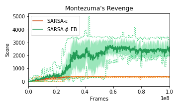
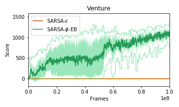
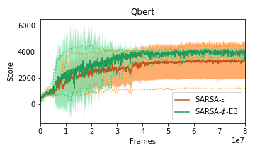
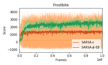
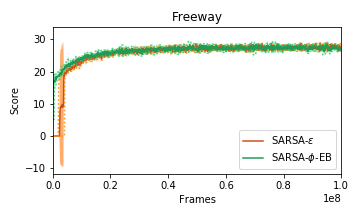
Figure 1: Average training scores for Sarsa-$\phi$-EB and the baseline Sarsa-$\epsilon$. Dashed lines are min/max scores. Shaded regions describe one standard deviation.

	Venture	Montezuma’s Revenge	Freeway	Frostbite	Q*bert
Sarsa-$\phi$-EB	1169.2	2745.4	0.0	2770.1	4111.8
Sarsa-$\epsilon$	0.0	399.5	29.9	1394.3	3895.3
DDQN-PC	N/A	3459	N/A	N/A	N/A
A3C+	0	142	27	507	15805
TRPO-Hash	445	75	34	5214	N/A
MP-EB	N/A	0	12	380	N/A
DDQN	98	0	33	1683	15088
DQN-PA	1172	0	33	3469	5237
Gorila	1245	4	12	605	10816
TRPO	121	0	16	2869	7733
Dueling	497	0	0	4672	19220

Table 1: Average evaluation score for leading algorithms. Sarsa-$\phi$-EB and Sarsa-$\epsilon$ were evaluated after 100M training frames on all games except Q*bert, for which they trained for 80M frames. DDQN-PC scores reflect evaluation after 100M training frames. The MP-EB agent was only trained for 20M frames. All other algorithms were evaluated after 200M frames. Leading scores are highlighted in bold.

In Montezuma’s Revenge, Sarsa-$\epsilon$ rarely leaves the first room. Its policy converges after an average of 20 million frames. Sarsa-$\phi$-EB continues to improve throughout training, visiting up to 14 rooms. The largest improvement over the baseline occurs in Venture. Sarsa-$\epsilon$ fails to score, while Sarsa-$\phi$-EB continues to improve throughout training. In Q*bert and Frostbite, the difference is less dramatic. These games have dense, well-shaped rewards that guide the agent’s path through state space and elide $\epsilon$-greedy’s inefficiency. Nonetheless, Sarsa-$\phi$-EB consistently outperforms Sarsa-$\epsilon$ throughout training so its cumulative reward is much higher.

In Freeway, Sarsa-$\phi$-EB with $\beta=0.05$ fails to match the performance of the baseline algorithm, but with $\beta=0.035$ it performs better (Figure 1 shows the learning curve for the latter). This sensitivity to the $\beta$ parameter likely results from the large number of unique Blob-PROST features that are active in Freeway, many of which are not relevant for finding the optimal policy. If $\beta$ is too high the agent is content to stand still and receive exploration bonuses for observing new configurations of traffic. This accords with our hypothesis that efficient optimistic exploration should involve measuring novelty with respect to task-relevant features.

In summary, Sarsa-$\phi$-EB with $\beta=0.05$ outperforms Sarsa-$\epsilon$ on all tested games except Freeway. Since both use the same feature set and RL algorithm, and differ only in their exploration policies, this is strong evidence that $\phi$-EB produces improvement over random exploration across a range of environments. This also supports our conjecture that using the same features for value function approximation and novelty estimation is an appropriate way to generalise visit-counts to the high-dimensional setting.

Comparison with Leading Algorithms

Table 1 compares our evaluation scores to Double DQN (DDQN) van Hasselt et al. (2016b), Double DQN with pseudocount (DDQN-PC) Bellemare et al. (2016), A3C+ Bellemare et al. (2016), DQN Pop-Art (DQN-PA) van Hasselt et al. (2016a), Dueling Network (Dueling) Wang et al. (2016), Gorila Nair et al. (2015), DQN with Model Prediction Exploration Bonuses (MP-EB) Stadie et al. (2015), Trust Region Policy Optimisation (TRPO) Schulman et al. (2015), and TRPO-AE-SimHash (TRPO-Hash) Tang et al. (2016). The most interesting comparisons for our purposes are with TRPO-Hash, DDQN-PC, A3C+, and MP-EB, because these algorithms all use exploration strategies that drive the agent to reduce its uncertainty. TRPO-Hash, DDQN-PC, and A3C+ are count-based methods, MP-EB seeks high model prediction error.

Our Sarsa-$\phi$-EB algorithm achieves an average score of 2745.4 on Montezuma: the second highest reported score. On this game it far outperforms every algorithm apart from DDQN-PC, despite only having trained for half the number of frames. Note that neither A3C+ nor TRPO-Hash achieves more than 200 points, despite their exploration strategies.

On Venture Sarsa-$\phi$-EB also achieves state-of-the-art performance. It achieves the third highest reported score despite its short training regime, and far outperforms A3C+ and TRPO-Hash. DDQN-PC evaluation scores are not given for Venture, but reported learning curves suggest Sarsa-$\phi$-EB performs much better here Bellemare et al. (2016). The performance of Sarsa-$\phi$-EB in Frostbite also seems competitive given the shorter training regime. Nonlinear algorithms perform better in Q*bert. In Freeway Sarsa-$\phi$-EB fails to score any points, for reasons already discussed.

6 Conclusion

We have introduced the $\phi$-Exploration Bonus method, a count-based optimistic exploration strategy that scales to high-dimensional environments. It is simpler to implement and less computationally demanding than some other proposals. Our evaluation shows that it improves upon $\epsilon$-greedy exploration on a variety of games, and that it is even competitive with leading exploration techniques developed for deep RL. Unlike other methods, it does not require the design of an exploration-specific state representation, but rather exploits the features used in the approximate value function. We have argued that computing novelty with respect to these task-relevant features is an efficient and principled way to generalise visit-counts for exploration. We conclude by noting that this reliance on the feature representation used for LFA is also a limitation. It is not obvious how a method like ours could be combined with the nonlinear function approximation techniques that have driven recent progress in RL. We hope the success of our simple method will inspire future work in this direction.

References

- Bellemare et al. [2013] Marc G Bellemare, Yavar Naddaf, Joel Veness, and Michael Bowling. The arcade learning environment: An evaluation platform for general agents. Journal of Artificial Intelligence Research, 47:253–279, 2013.
- Bellemare et al. [2016] Marc G. Bellemare, Sriram Srinivasan, Georg Ostrovski, Tom Schaul, David Saxton, and Rémi Munos. Unifying count-based exploration and intrinsic motivation. CoRR, abs/1606.01868, 2016.
- Kakade [2003] Sham Machandranath Kakade. On the Sample Complexity of Reinforcement Learning. PhD thesis, University College London, 2003.
- Kolter and Ng [2009] J Zico Kolter and Andrew Y Ng. Near-Bayesian exploration in polynomial time. International Conference on Machine Learning, pages 513–520, 2009.
- Lai and Robbins [1985] Tze Leung Lai and Herbert Robbins. Asymptotically efficient adaptive allocation rules. Advances in Applied Mathematics, 6(1):4–22, 1985.
- Liang et al. [2016] Yitao Liang, Marlos C Machado, Erik Talvitie, and Michael Bowling. State of the art control of Atari games using shallow reinforcement learning. In Autonomous Agents and Multi-Agent Systems, 2016.
- Mnih et al. [2015] Volodymyr Mnih, Koray Kavukcuoglu, David Silver, Andrei a Rusu, Joel Veness, Marc G Bellemare, Alex Graves, Martin Riedmiller, Andreas K Fidjeland, Georg Ostrovski, Stig Petersen, Charles Beattie, Amir Sadik, Ioannis Antonoglou, Helen King, Dharshan Kumaran, Daan Wierstra, Shane Legg, and Demis Hassabis. Human-level control through deep reinforcement learning. Nature, 518(7540):529–533, 2015.
- Mnih et al. [2016] Volodymyr Mnih, Adrià Puigdomènech Badia, Mehdi Mirza, Alex Graves, Timothy P Lillicrap, Tim Harley, David Silver, and Koray Kavukcuoglu. Asynchronous methods for deep reinforcement learning. In International Conference on Machine Learning, 2016.
- Nair et al. [2015] Arun Nair, Praveen Srinivasan, Sam Blackwell, Cagdas Alcicek, Rory Fearon, Alessandro De Maria, Vedavyas Panneershelvam, Mustafa Suleyman, Charles Beattie, Stig Petersen, Shane Legg, Volodymyr Mnih, Koray Kavukcuoglu, and David Silver. Massively parallel methods for deep reinforcement learning. CoRR, abs/1507.04296, 2015.
- Osband et al. [2016a] Ian Osband, Charles Blundell, Alexander Pritzel, and Benjamin Van Roy. Deep exploration via bootstrapped DQN. CoRR, abs/1602.04621, 2016.
- Osband et al. [2016b] Ian Osband, Benjamin Van Roy, and Zheng Wen. Generalization and exploration via randomized value functions. International Conference on Machine Learning, pages 1–26, 2016.
- Ostrovski et al. [2017] Georg Ostrovski, Marc G. Bellemare, Aäron van den Oord, and Rémi Munos. Count-based exploration with neural density models. CoRR, abs/1703.01310, 2017.
- Schulman et al. [2015] John Schulman, Sergey Levine, Philipp Moritz, Michael I. Jordan, and Pieter Abbeel. Trust region policy optimization. CoRR, abs/1502.05477, 2015.
- Stadie et al. [2015] Bradly C. Stadie, Sergey Levine, and Pieter Abbeel. Incentivizing exploration in reinforcement learning with deep predictive models. CoRR, abs/1507.00814, 2015.
- Strehl and Littman [2004] A. L. Strehl and M. L. Littman. An empirical evaluation of interval estimation for Markov decision processes. In 16th IEEE International Conference on Tools with Artificial Intelligence, pages 128–135, 2004.
- Strehl and Littman [2008] Alexander L Strehl and Michael L Littman. An analysis of model-based interval estimation for Markov decision processes. Journal of Computer and System Sciences, 74(8):1309–1331, 2008.
- Strehl et al. [2009] Alexander L Strehl, Lihong Li, and Michael L Littman. Reinforcement Learning in Finite MDPs : PAC Analysis. Journal of Machine Learning Research, 10:2413–2444, 2009.
- Sutton and Barto [1998] R.S. Sutton and A.G. Barto. Reinforcement Learning: An Introduction. IEEE Transactions on Neural Networks, 9(5):1054–1054, 1998.
- Sutton [1990] Richard S. Sutton. Integrated architecture for learning, planning, and reacting based on approximating dynamic programming. In International Conference on Machine Learning, pages 216–224, 1990.
- Tang et al. [2016] Haoran Tang, Rein Houthooft, Davis Foote, Adam Stooke, Xi Chen, Yan Duan, John Schulman, Filip De Turck, and Pieter Abbeel. #Exploration: A study of count-based exploration for deep reinforcement learning. CoRR, abs/1611.04717, 2016.
- van Hasselt et al. [2016a] Hado van Hasselt, Arthur Guez, Matteo Hessel, and David Silver. Learning values across many orders of magnitude. CoRR, abs/1602.07714, 2016.
- van Hasselt et al. [2016b] Hado van Hasselt, Arthur Guez, and David Silver. Deep reinforcement learning with double Q-learning. In AAAI, 2016.
- Veness et al. [2012] Joel Veness, Kee Siong Ng, Marcus Hutter, and Michael Bowling. Context tree switching. In IEEE Data Compression Conference, pages 327–336, 2012.
- Wang et al. [2016] Ziyu Wang, Nando de Freitas, Tom Schaul, Matteo Hessel, Hado van Hasselt, and Marc Lanctot. Dueling network architectures for deep reinforcement learning. In International Conference on Machine Learning, 2016.