Ground-state ionization energies of boronlike ions

Abstract

High-precision QED calculations of the ground-state ionization energies are performed for all boronlike ions with the nuclear charge numbers in the range $16\leqslant Z\leqslant 96$. The rigorous QED calculations are performed within the extended Furry picture and include all many-electron QED effects up to the second order of the perturbation theory. The contributions of the third- and higher-order electron-correlation effects are accounted for within the Breit approximation. The nuclear recoil and nuclear polarization effects are taken into account as well. In comparison with the previous evaluations of the ground-state ionization energies of boronlike ions the accuracy of the theoretical predictions has been improved significantly.

I Introduction

Quantum electrodynamics (QED) is well known as a powerful tool to describe systems of electrically charged particles interacting via the electromagnetic forces. Since the beginning of 1950’s when this theory was formulated it had a great success in interpreting and predicting experimental results. With a possibility to study heavy few-electron ions experimentally, which appeared in the middle of 1980’s Beyer and Shevelko (2003), these systems became the subject of extensive theoretical investigations, for review see Refs. Mohr et al. (1998); Sapirstein and Cheng (2008); Shabaev (2008); Glazov et al. (2011); Volotka et al. (2013) and references therein. In contrast to light atoms and ions, where the binding-strength parameter of the nucleus $\alpha Z$ ($\alpha$ is the fine structure constant and $Z$ is the nuclear charge number) can be used along with $\alpha$ to evaluate QED effects by perturbation theory, for high-$Z$ systems this parameter is not small and, therefore, all the calculations must be performed without any expansion in $\alpha Z$. On the other hand, since the number of electrons $N$ in highly charged ions is much smaller than the nuclear charge number $Z$, it is possible to calculate interelectronic-interaction effects using the perturbation theory in the parameter $1/Z$. This approach leads to quantum electrodynamics in the Furry picture Furry (1951), where the interaction of electrons with nucleus is treated to all orders in $\alpha Z$. Due to rather simple electronic structure of heavy few-electron ions as compared to neutral atoms the uncertainty of the electron-correlation corrections doesn’t prevent one to probe QED effects in such systems. Therefore, highly charged ions are ideal candidates to examine new theoretical methods developed for description of bound-electron systems.

State-of-the-art QED calculations of the energy levels in highly charged ions include all relevant contributions up to the second order in $\alpha$. To date, the corresponding calculations have been performed for highly charged ions with the number of electrons from one to five  Yerokhin and Shabaev (2015); Artemyev et al. (2005); Yerokhin et al. (2001); Kozhedub et al. (2010); Sapirstein and Cheng (2011); Malyshev et al. (2014, 2015); Artemyev et al. (2007, 2013); Malyshev et al. . High-precision measurements of the binding and transition energies which are sensitive to the second-order corrections confirm predictions made by QED theory to a high level of accuracy  Schweppe et al. (1991); Stöhlker et al. (1993); Beiersdorfer et al. (1998a, b); Bosselmann et al. (1999); Stöhlker et al. (2000); Brandau et al. (2003); Draganić et al. (2003); Gumberidze et al. (2004, 2005); Beiersdorfer et al. (2005); Mäckel et al. (2011); Kubiček et al. (2014); Bernhardt et al. (2015); Beiersdorfer and Brown (2015); Epp et al. (2015); Kraft-Bermuth et al. (2017) and allow one to test bound-state QED in the strong-field regime. In future, several new facilities are planned or already commenced aiming for further improvement of the experimental accuracy. Among them are the high-precision X-ray spectroscopy projects FOCAL Beyer et al. (2015) and maXs calorimeter Hengstler et al. (2015) implementing at the CRYRING@ESR facility in GSI Lestinsky et al. (2016) as well as the mass-spectrometry project PENTATRAP Repp et al. (2012); Roux et al. (2012) in Heidelberg. In view of this, further extension and improvement of ab initio QED calculations are of great importance.

The present investigation is focused on five-electron boronlike ions. There are many relativistic calculations of the excited state energies of boronlike ions, see, e.g., Refs. Safronova et al. (1996, 1998); Koc (2005); Rynkun et al. (2012). However, the many-electron QED effects were considered within some one-electron or semiempirical approximations in these studies. The rigorous QED evaluation of the $2p_{3/2}-2p_{1/2}$ fine-structure splitting in boronlike ions was performed only in Refs. Artemyev et al. (2007, 2013). The main goal of the present paper is to calculate the ionization energies of the $1s^{2}2s^{2}2p_{1/2}$ ground state for the nuclear charge number in the wide range $16\leqslant Z\leqslant 96$. The numerical approach that we use is generally similar to the procedure discussed in Ref. Malyshev et al. (2015), where the calculations of the ground-state ionization energies for berylliumlike ions have been performed. The approach combines the first and second orders of the QED perturbation theory with the higher-order electron-correlation contributions evaluated within the Breit approximation. Taking into account the results of Ref. Artemyev et al. (2013) one can easily obtain the ionization energies for the first excited state $1s^{2}2s^{2}2p_{3/2}$ of boronlike ions, for this one needs to add the transition energies of Ref. Artemyev et al. (2013) to the the ground-state ionization energies presented in this work.

The paper is organized as follows. In Sec. II we describe the procedure which was used to evaluate the ionization energies. In Sec. III our numerical results are presented and compared with the theoretical predictions obtained in previous works.

The relativistic units ($\hbar=c=1$) and the Heaviside charge unit ($\alpha=e^{2}/4\pi,e<0$) are used throughout the paper.

II Basic formulas

In highly charged ions the number of electrons $N$ is much smaller than the nuclear charge number $Z$. As a result, the interelectronic interaction is suppressed by the factor $1/Z$ compared to the interaction of the individual electrons with the Coulomb field of the nucleus. Therefore, a good starting point for systematic description of these systems within QED is the Furry picture Furry (1951). In this framework one starts from the assumption that one-electron wave functions obey the Dirac equation

$$\left[-i\bm{\alpha}\cdot\nabla+\beta m+V(\bm{r})\right]\psi_{n}(\bm{r})=\varepsilon_{n}\psi_{n}(\bm{r}),$$ (1)

where in the simplest case $V(\bm{r})$ is the potential of the nucleus $V_{\rm{nucl}}(\bm{r})$. Alternatively, one can choose the potential $V(\bm{r})$ to be an effective potential, that is the sum of the nuclear potential and some screening potential:

$$V(\bm{r})\rightarrow V_{\rm{eff}}(\bm{r})=V_{\rm{nucl}}(\bm{r})+V_{\rm{scr}}(\bm{r}).$$ (2)

The screening potential is employed to take into account the interelectronic-interaction effects partly from the very beginning. In the present work we follow this alternative choice of the zeroth order approximation, which is known as the extended Furry picture. This approach accelerates the convergence of the perturbation series and was applied successfully to high-precision calculations of various atomic properties Sapirstein and Cheng (2002, 2011); Chen et al. (2006); Artemyev et al. (2007); Yerokhin et al. (2007a); Kozhedub et al. (2010); Artemyev et al. (2013); Sapirstein and Cheng (2003a, 2006); Oreshkina et al. (2007); Kozhedub et al. (2007); Volotka et al. (2008); Glazov et al. (2006); Volotka et al. (2014); Zubova et al. (2016). In addition, the use of the effective potential improves significantly the numerical accuracy of the calculations, since it can remove the quasi-degeneracy of the states with the same symmetry, which may take place if the pure Coulomb potential is employed in the initial approximation.

We note here, that the zeroth-order results depend strongly on the choice of the effective potential. If one could treat the QED and correlation effects to all orders of the perturbation theory, the final results would be independent on screening potential employed. In practice, however, state-of-the-art calculations for highly charged ions are limited by the consideration of the second-order QED corrections. The deviations of the final results obtained with the use of the different screening potentials can provide an estimation of the uncalculated higher-order contributions.

In the present work we employ several different types of the screening potential. The first one is the core-Hartree (CH) potential induced by the $1s^{2}2s^{2}$ core. This potential can be constructed from the radial charge density of the $1s$ and $2s$ electrons:

$$V_{\rm CH}(r)=\alpha\int_{0}^{\infty}dr^{\prime}\frac{1}{r_{>}}\rho_{\rm CH}(r^{\prime}),$$ (3)

$$\rho_{\rm CH}(r)=2\sum_{c=1s,2s}\left[G_{c}^{2}(r)+F_{c}^{2}(r)\right],\qquad\int_{0}^{\infty}\rho_{\rm CH}(r)dr=N-1,$$ (4)

where $N=5$ is the total number of the electrons, $r_{>}={\rm max}(r,r^{\prime})$, $G/r$ and $F/r$ are the large and small radial components of the Dirac wave function

$$\psi(\bm{r})=\frac{1}{r}{\left(\begin{array}[]{c}G(r)\Omega_{\kappa m}(\bm{\hat{r}})\\ iF(r)\Omega_{-\kappa m}(\bm{\hat{r}})\\ \end{array}\right)},$$ (5)

$\Omega_{\kappa m}$ is the spin-angular spinor, and $\bm{\hat{r}}=\bm{r}/r$.

The next three potentials are built for the $1s^{2}2s^{2}2p_{1/2}$ electron configuration. The local Dirac-Fock (LDF) potential is generated from the wave functions evaluated within the Dirac-Fock approximation Shabaev et al. (2005) and reproduces the energies and wave functions of the $2p_{1/2}$ state at the corresponding level. The Kohn-Sham (KS) and Perdew-Zunger (PZ) potentials are formulated in the framework of the density-functional theory. The KS potential is given by the following expression Kohn and Sham (1965):

$$V_{\rm{KS}}(r)=\alpha\int_{0}^{\infty}dr^{\prime}\frac{1}{r_{>}}\rho_{t}(r^{\prime})-\frac{2}{3}\frac{\alpha}{r}\left(\frac{81}{32\pi^{2}}r\rho_{t}(r)\right)^{1/3},$$ (6)

where $\rho_{t}$ is the radial density of all electrons:

$$\rho_{t}(r)=\rho_{\rm CH}(r)+\left[G_{2p_{1/2}}^{2}(r)+F_{2p_{1/2}}^{2}(r)\right],\qquad\int_{0}^{\infty}\rho_{t}(r)dr=N.$$ (7)

The second term in Eq. (6) describes the exchange part of the interelectronic interaction. We use the Latter correction Latter (1955) to restore the proper asymptotic behavior of the KS potential at large distances. The PZ potential contains an additional correlation term in comparison to the KS potential Perdew and Zunger (1981). The self-interaction correction for the PZ potential is taken into account according to Ref. Perdew and Zunger (1981). In order to expand the range of the initial approximations used to evaluate ionization energies of boronlike ions we consider the second PZ potential generated for the $1s^{2}2s^{2}2p_{3/2}$ electron configuration. To distinguish those two kinds of the PZ potential in what follows we will add the indices 1 and 3 to label the potentials constructed for the configurations with the $2p_{1/2}$ and $2p_{3/2}$ electrons, respectively. Therefore, the total number of the screening potentials used in the present work is equal to five. We note, that at large distances $r$ all the screening potentials behave like $N_{\rm scr}\alpha/r$, where $N_{\rm scr}=N-1$.

Solving Eq. (1) with an effective potential (2) for the state $2p_{1/2}$ one can obtain the zeroth-order approximation for the ionization energy $E^{(0)}_{\rm Dirac}=\varepsilon_{2p_{1/2}}-mc^{2}$. The QED and electron-correlation contributions have to be taken into account by a perturbation theory. To derive formal expressions for the terms of the perturbation series we use the two-time Green function (TTGF) method Shabaev (2002). It should be noted that within the extended Furry picture the potential $\delta V(\bm{r})=-V_{\rm{scr}}(\bm{r})$ is to be added into the QED interaction Hamiltonian. The counterterm $\delta V(\bm{r})$ must be accounted for perturbatively in order to avoid the double counting of the screening effects. In order to perform bound-state QED calculations one needs a quasicomplete basis set of the one-electron solutions of the Dirac equation to have a spectral representation of the Dirac-Coulomb Green function

$$G(\omega,\bm{r}_{1},\bm{r}_{2})=\sum_{n}\frac{\psi_{n}(\bm{r}_{1})\psi^{\dagger}_{n}(\bm{r}_{2})}{\omega-\varepsilon_{n}(1-i0)}.$$ (8)

The basis wave functions were constructed from the B-splines Johnson et al. (1988) with the use of the dual kinetic balance (DKB) approach Shabaev et al. (2004).

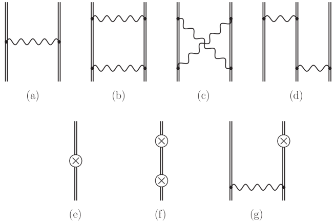
Figure 1: The interelectronic-interaction diagrams in the extended Furry picture. The double line denotes the electron propagator in the effective potential (2). The wavy line corresponds to the photon propagator. The symbol $\otimes$ represents the local screening potential counterterm $\delta V(\bm{r})=-V_{\rm{scr}}(\bm{r})$.

The evaluation of the ionization energies of boronlike ions can be accomplished in several steps. At first, we will discuss the calculation of the interelectronic-interaction corrections. As it was mentioned above, one can account for the electron-electron interaction partly replacing the potential of the nucleus in Eq. (1) with some effective potential. The remaining part of the interelectronic interaction is to be considered within the perturbation theory. In Fig. 1 the set of the first- and second-order Feynman diagrams describing the interelectronic interaction is shown. The double line corresponds to the electron propagator in the effective potential (2). The wavy line represents the photon propagator. Finally, the circle with a cross depicts the counterterm $\delta V(\bm{r})$. The ionization energy of the $2p_{1/2}$ electron can be obtained by subtracting the binding energy of the Be-like ion from the binding energy of the corresponding B-like ion. The diagrams with only core electrons as incoming (outgoing) electron lines cancels each other in this difference and don’t contribute to the ionization energy under consideration. Therefore, in what follows we will work only with the diagrams where one of the incoming (outgoing) electron lines corresponds to the $2p_{1/2}$ valence electron. The formulas for the contributions of the first- and second-order diagrams shown in Fig. 1 can be derived with the use of the TTGF method. The formal expressions for all the relevant contributions are presented in Appendix A.

At the next stage we have to evaluate the interelectronic-interaction contributions of the third and higher orders, which are also important. In the present work we have calculated these corrections within the Breit approximation using two different approaches. First of all, as in Refs. Malyshev et al. (2014, 2015), we have employed the configuration-interaction Dirac-Fock-Sturm (CI-DFS) method Bratzev et al. (1977); Tupitsyn et al. (2003) to solve the Dirac-Coulomb-Breit (DCB) equation yielding the total binding energy. In order to separate the desired third- and higher-order contributions from the total CI-DFS results the following procedure has been used. A free parameter $\lambda$ is introduced into the DCB Hamiltonian

$$H_{\rm DCB}(\lambda)=\Lambda^{(+)}\Big{[}H_{0}+\lambda V_{\rm int}\Big{]}\Lambda^{(+)},$$ (9)

$$H_{0}=\sum_{i}\left[\bm{\alpha}_{i}\cdot\bm{p}_{i}+\beta_{i}m+V_{\rm eff}^{(i)}\right],$$ (10)

$$V_{\rm int}=\sum_{i<j}\left[V_{\rm C}^{(i,j)}+V_{\rm B}^{(i,j)}\right]-\sum_{i}V_{\rm scr}^{(i)},$$ (11)

$$V_{\rm C}^{(i,j)}=\frac{\alpha}{r_{ij}},\qquad V_{\rm B}^{(i,j)}=-\frac{\alpha}{2}\left[\frac{\bm{\alpha}_{i}\cdot\bm{\alpha}_{j}}{r_{ij}}+\frac{(\bm{\alpha}\cdot\bm{r}_{ij})(\bm{\alpha}_{j}\cdot\bm{r}_{ij})}{r_{ij}^{3}}\right],$$ (12)

where $\Lambda^{(+)}$ is the product of the one-electron projectors on the positive-energy states (which correspond to the potential $V_{\rm eff}$), $H_{0}$ is the unperturbed Hamiltonian, $V_{\rm int}$ describes the interaction of the electrons with each other and with the counterterm potential $-V_{\rm scr}$, $V_{\rm C}$ and $V_{\rm B}$ are the Coulomb and Breit parts of the electron-electron interaction operator in the Breit approximation, respectively. The Hamiltonian (9) coincides with the original DCB Hamiltonian for $\lambda=1$. The energy $E$ evaluated within the CI-DFS method becomes a function of the parameter $\lambda$ when the Hamiltonian (9) is used in the calculations. One can expand the energy $E(\lambda)$ in powers of $\lambda$

$$E(\lambda)=E^{(0)}+\lambda E^{(1)}+\lambda^{2}E^{(2)}+\sum_{k}^{\infty}\lambda^{k}E^{(k)},$$ (13)

$$E^{(k)}=\left.\frac{1}{k!}\frac{{\rm d}^{k}}{{\rm d}\lambda^{k}}E(\lambda)\right|_{\lambda=0}.$$ (14)

It can be seen that the coefficients $E^{(k)}$ correspond to the different orders of the perturbation theory. Therefore, for the contribution of the third and higher orders

$$E^{(\geqslant 3)}=\sum_{k=3}^{\infty}E^{(k)}$$ (15)

one can obtain the following expression in the framework of the CI-DFS approach

$$E^{(\geqslant 3)}=\left.E(\lambda)\right|_{\lambda=1}-E^{(0)}-E^{(1)}-E^{(2)},$$ (16)

where the coefficient $E^{(0)}$, $E^{(1)}$, and $E^{(2)}$ have to be determined numerically according to Eq. (14).

Along with the CI-DFS calculations, in the present work the higher-order interelectronic-interaction corrections have been evaluated also with the use of the recursive formulation of the perturbation theory. The detailed description of this approach is presented in our recent work Glazov et al. . Below we consider its basic principles.

While the perturbation expansion for the energy is given by Eq. (13) with $\lambda=1$, we have the following expansion for the many-electron wave function $|A\rangle$ of the state under consideration

$$|A\rangle =\sum_{k=0}^{\infty}|A^{(k)}\rangle=\sum_{k=0}^{\infty}\sum_{N}|N^{(0)}\rangle\langle N^{(0)}|A^{(k)}\rangle\,.$$ (17)

The finite basis set of the many-electron wave functions $|N^{(0)}\rangle$ consists of the Slater determinants, being the eigenfunctions of $H_{0}$ with the eigenvalues $E_{N}^{(0)}$,

$$\Lambda^{(+)}H_{0}\Lambda^{(+)}|N^{(0)}\rangle=E_{N}^{(0)}|N^{(0)}\rangle\;.$$ (18)

The Slater determinants are made of the one-electron wave functions constructed within the DKB method Shabaev et al. (2004). It provides the same zeroth-order approximation that is used for the calculation of the first- and second-order QED contributions assuming the same choice of the screening potential. The energy corrections $E^{(k)}$ and the coefficients $\langle N^{(0)}|A^{(k)}\rangle$ can be found via the recursive system of equations,

$$E^{(k)}= \sum_{M}\left\langle A^{(0)}\left|\vphantom{A^{(0)}}V_{\rm int}\vphantom{M^{(0)}}\right|M^{(0)}\right\rangle\langle M^{(0)}|A^{(k-1)}\rangle-\sum_{j=1}^{k-1}E^{(j)}\langle A^{(0)}|A^{(k-j)}\rangle\,,$$ (19)

$${\left.\langle N^{(0)}|A^{(k)}\rangle\right|}_{N\neq A}=\, \frac{1}{E^{(0)}-E_{N}^{(0)}}\left[\sum_{M}\left\langle N^{(0)}\left|\vphantom{N^{(0)}}V_{\rm int}\vphantom{M^{(0)}}\right|M^{(0)}\right\rangle\langle M^{(0)}|A^{(k-1)}\rangle-\sum_{j=1}^{k-1}E^{(j)}\langle N^{(0)}|A^{(k-j)}\rangle\right]\,,$$ (20)

$$\langle A^{(0)}|A^{(k)}\rangle=\, -\frac{1}{2}\,\sum_{j=1}^{k-1}\sum_{M}\langle A^{(j)}|M^{(0)}\rangle\langle M^{(0)}|A^{(k-j)}\rangle\,,$$ (21)

with the initial values,

$${\left.\langle N^{(0)}|A^{(0)}\rangle\right|}_{N\neq A}=0\,,\;\;\;\;\langle A^{(0)}|A^{(0)}\rangle=1\,.$$ (22)

The matrix elements of $V_{\rm int}$ with the Slater determinants are reduced to the one- and two-electron matrix elements according to the well-known combinatorial formulas. Each step of the recursion comprises only one-fold summation over the basis set for each $\langle N^{(0)}|A^{(k)}\rangle$, in contrast to the conventional form of the perturbation theory. It makes the procedure computationally efficient and allows one to access essentially arbitrary high order of the perturbation theory. The desired contribution of the third- and higher-order interelectronic-interaction effects $E^{(\geqslant 3)}$ can be obtained by the direct summation in Eq. (15). The summation is terminated according to the total accuracy that one aims at. The energies obtained by means of the CI-DFS method and the direct summation of the perturbation series are found to be in a good agreement. The application of the fully independent approaches based on the completely different grounds allows one to perform more reliable estimation of the accuracy of the calculations.

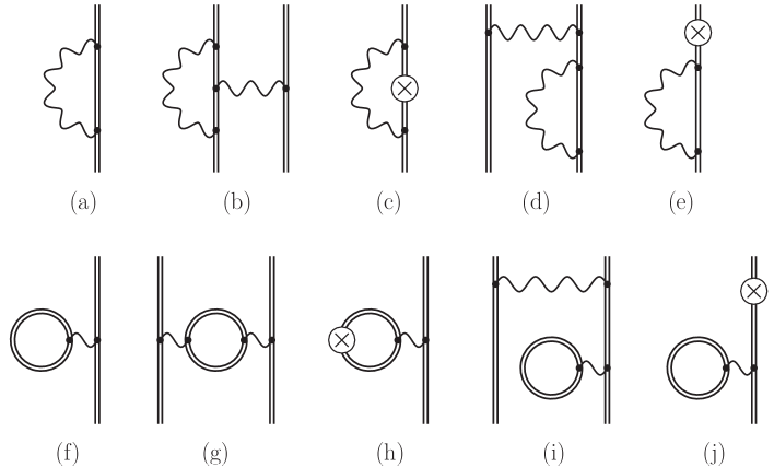
Figure 2: First- and second-order QED diagrams (excluding the one-electron two-loop diagrams) in the extended Furry picture. The notations are the same as in Fig. 1.

At the next step one has to account for the radiative corrections. All the necessary one-electron and many-electron one-loop Feynman diagrams are shown in Fig. 2. The first line in Fig. 2 presents the self-energy (SE) diagrams, in the second line the vacuum-polarization (VP) diagrams are given. The formal expressions for the corresponding corrections in the extended Furry picture can be readily obtained in the framework of the TTGF method. For convenience, all the formulas needed for evaluation of the ionization energies of boronlike ions are collected in Appendix B.

We note, that in the present work in order to calculate the first-order self-energy correction for the $2p_{1/2}$ electron moving in the effective potential (2) we employ the procedure described in Refs. Artemyev et al. (2007, 2013). The approach suggested there is a modification of the standard scheme (see Ref. Artemyev et al. (2013) and references therein) for the evaluation of the SE contributions. According to the standard scheme one has to expand the Dirac-Coulomb Green function in powers of the potential $V_{\rm{eff}}$ (see Eq. (38) in Appendix B), and this expansion gives rise to the zero-, one-, and many-potential terms of the total SE correction. The zero- and one-potential terms are both divergent and should be renormalized. The renormalization procedure is discussed, e.g., in Ref. Yerokhin and Shabaev (1999), and after its application the calculation of the zero- and one-potential terms is straightforward. The many-potential term corresponds to the part with two or more potentials in the expansion of the Dirac-Coulomb Green function, and its evaluation is the most time consuming. The calculation of the many-potential term for the $2p_{j}$ states in low-$Z$ ions in the case of the extended Furry picture is complicated because of the slow convergence of the partial-wave expansion for this contribution, see Ref. Artemyev et al. (2013) for details. In Refs. Artemyev et al. (2007, 2013) it was suggested to separate the part of the many-potential term that defines the slow convergence, namely the two-potential term, that is the contribution with two potentials in the Green function expansion. The separated two-potential term can be evaluated to a high accuracy using the analytical representation for the free-electron propagator. After the evaluation of the two-potential term is accomplished the calculation of the remaining part of the many-potential term does not cause any difficulties.

In order to control the total accuracy of the one-electron SE contribution, we have also performed the calculations employing the approach described, e.g., in Ref. Kozhedub et al. (2010) in addition to the method of Refs. Artemyev et al. (2007, 2013). By means of the standard procedure Yerokhin and Shabaev (1999) we have evaluated the screening effect to the first-order SE correction, that is the difference between this contribution calculated with and without the screening potential. By adding the self-energy correction evaluated for the electron in the Coulomb field Yerokhin and Shabaev (2015), we have obtained the results which are in a good agreement with the values calculated by the first approach.

Next, we have to take into account the contributions corresponding to the two-loop one-electron diagrams. The consideration of these corrections completes the rigorous QED treatment of the ground-state ionization energies of boronlike ions to the second order in $\alpha$ within the Furry picture. The nonperturbative in $\alpha Z$ evaluation of the two-loop diagrams is a very difficult problem, which is not fully accomplished yet. The most significant achievement in this field is related to the calculation of the two-loop self-energy correction by Yerokhin et al. Yerokhin et al. (2003, 2006, 2007b); Yerokhin (2009, 2010). The contributions of the diagrams with closed fermion loops have been considered in Refs. Mallampalli and Sapirstein (1996); Persson et al. (1996); Beier et al. (1997); Plunien et al. (1998); Yerokhin et al. (2008), the free-loop approximation has been used in a part of these terms. In the present work to account for the two-loop one-electron corrections we use the results from  Refs. Yerokhin et al. (2008); Yerokhin and Shabaev (2015).

In all the contributions discussed so far the nucleus was considered as a motionless source of the external electrical field, i.e., it was assumed that the nucleus has the infinite mass. The high-precision calculations of highly-charged ions have to go beyond this external field approximation and account for the nuclear recoil corrections. The full relativistic theory of the nuclear recoil effect to the first order in $m/M$ ($M$ is the nuclear mass) and to all orders in $\alpha Z$ can be formulated only within QED Shabaev (1985, 1988, 1998); Adkins et al. (2007). The lowest-order relativistic nuclear recoil corrections can be evaluated by averaging the operator  Shabaev (1985, 1988); Palmer (1987)

$$H_{M}=\frac{1}{2M}\sum_{i,j}\left\{\bm{p}_{i}\cdot\bm{p}_{j}-\frac{\alpha Z}{r_{i}}\left[\bm{\alpha}_{i}+\frac{(\bm{\alpha}_{i}\cdot\bm{r}_{i})\bm{r}_{i}}{r_{i}^{2}}\right]\cdot\bm{p}_{j}\right\}.$$ (23)

In the present work we calculate the expectation values of the operator (23) with the many-electron wave functions obtained in the framework of the CI-DFS method. Such an approach allows one to take into account the nuclear recoil effect within the Breit approximation to all orders in $1/Z$. This correction has been evaluated also with the wave functions obtained within the recursive perturbation theory (17). The contribution of the $k$-th order in $1/Z$ is given by,

$$\Delta E_{\rm rec,Breit}^{(k)}= \sum_{j=0}^{k}\sum_{M,N}\langle A^{(j)}|M^{(0)}\rangle\left\langle M^{(0)}\left|\vphantom{M^{(0)}}H_{M}\vphantom{N^{(0)}}\right|N^{(0)}\right\rangle\langle N^{(0)}|A^{(k-j)}\rangle\,,$$ (24)

where the coefficients $\langle A^{(j)}|M^{(0)}\rangle\equiv\langle M^{(0)}|A^{(j)}\rangle$ are evaluated through Eqs. (19), (20), and (21). The results of both calculations were found to be in a good agreement with each other.

The nuclear recoil corrections which are beyond the Breit approximation are referred to as the QED nuclear recoil effects. We have evaluated these contributions to the zeroth order in $1/Z$. The one-electron part of the QED nuclear recoil corrections in the case of the point nucleus can be expressed as follows  Shabaev (1985, 1988):

$$\Delta E_{\rm 1el}^{\rm rec} = \frac{i}{2\pi M}\int_{-\infty}^{\infty}\!d\omega\,\left\langle v\left|\left({\bm{D}}(\omega)-\frac{[{\bm{p}},V]}{\omega+i0}\right)\right.\right.$$ (25)

$$\times G(\omega+\varepsilon_{v})\left.\left.\left({\bm{D}}(\omega)+\frac{[{\bm{p}},V]}{\omega+i0}\right)\right|v\right\rangle,$$

where ${\bm{p}}$ is the momentum operator, $D_{m}(\omega)=-4\pi\alpha Z\alpha_{l}D_{lm}(\omega)$, and $D_{lm}$ is the transverse part of the photon propagator considered in the Coulomb gauge. The two-electron part has the form Shabaev (1988)

$$\Delta E_{\rm 2el}^{\rm rec} = \frac{1}{M}\sum_{c=1s,2s}\sum_{\mu_{c}}\Big{\{}\langle v|{\bm{p}}|c\rangle\langle c|{\bm{D}}(\Delta)-{\bm{D}}(0)|v\rangle$$ (26)

$$+\langle v|{\bm{D}}(\Delta)-{\bm{D}}(0)|c\rangle\langle c|{\bm{p}}|v\rangle-\langle v|{\bm{D}}(\Delta)|c\rangle\langle c|{\bm{D}}(\Delta)|v\rangle\Big{\}},$$

where $\Delta=\varepsilon_{v}-\varepsilon_{c}$. One can partly take into account the nuclear size corrections to the QED nuclear recoil contributions (25) and (26) by replacing the potential $V=-\alpha Z/r$, the Green function $G$, the Dirac energies and wave functions of the point nucleus with the corresponding quantities for the extended nucleus Shabaev (1998). For the $1s$ and $2s$ states in hydrogenlike ions such calculations were performed in Refs. Shabaev et al. (1998, 1999), see also Ref. Aleksandrov et al. (2015). In the present paper, as in Refs. Orts et al. (2006); Malyshev et al. (2015); Zubova et al. (2016), we have evaluated the QED nuclear recoil corrections (25) and (26) for the effective potential (2) to account for the screening effects partly.

Finally, we have to consider the nuclear polarization corrections for high-$Z$ ions. These contributions result from the electron-nucleus interactions that include the excited intermediate nuclear states. We have used the data from Refs. Plunien et al. (1991); Plunien and Soff (1995); Nefiodov et al. (1996, 2002); Volotka and Plunien (2014) and the prescriptions from Ref. Yerokhin and Shabaev (2015) to take into account the nuclear polarization effects.

Summarizing the description of the numerical approach which we use to evaluate the ground-state ionization energies in boronlike ions it is worth noting that the calculations of the many-electron QED corrections in Figs. 1 and 2 have been carried out using both Feynman and Coulomb gauges for the electron-electron interaction propagator. The results of both calculations are in a good agreement with each other. To describe the nuclear charge distribution we use the Fermi model with a thickness parameter equaled to 2.3 fm. The nuclear radii are taken from Ref. Angeli and Marinova (2013) for the most abundant isotopes. In the cases of $Z$ for which the data are absent in Ref. Angeli and Marinova (2013) we have used the root-mean-square radii obtained by the approximate formula from Ref. Johnson and Soff (1985) with a $1\%$ uncertainty prescribed.

III Numerical results and discussions

Table 1: Interelectronic-interaction contributions of the 3rd and higher orders to the ionization energies (in eV) of the ground state in boronlike calcium, xenon, and uranium with the LDF and PZ3 potentials. The results of the CI-DFS calculations are given for comparison.

	$Z=20$				$Z=54$				$Z=92$
PT order	LDF		PZ3		LDF		PZ3		LDF		PZ3
3	0.	3401	0.	4133	$-$0.	9392	$-$0.	4625	$-$3.	0172	$-$2.	4786
4	$-$0.	5794	$-$0.	5313	$-$0.	1667	$-$0.	1973	0.	4857	0.	3527
5	0.	1708	0.	1260	0.	0950	0.	0494	0.	0058	0.	0133
6	0.	0544	0.	0564	$-$0.	0065	0.	0055	$-$0.	0356	$-$0.	0244
7	$-$0.	0581	$-$0.	0436	$-$0.	0062	$-$0.	0036	0.	0129	0.	0072
8	0.	0102	0.	0032	0.	0017	$-$0.	0000	$-$0.	0019	$-$0.	0007
9	0.	0090	0.	0077	0.	0003	0.	0003	$-$0.	0005	$-$0.	0003
10	$-$0.	0056	$-$0.	0030	$-$0.	0002	$-$0.	0000	0.	0004	0.	0002
11	$-$0.	0001	$-$0.	0007	0.	0000	$-$0.	0000	$-$0.	0001	$-$0.	0000
12	0.	0013	0.	0008	0.	0000	0.	0000	$-$0.	0000	$-$0.	0000
13	$-$0.	0004	$-$0.	0001	$-$0.	0000	0.	0000	0.	0000	0.	0000
14	$-$0.	0002	$-$0.	0001	$-$0.	0000	$-$0.	0000	0.	0000	$-$0.	0000
15	0.	0001	0.	0000	0.	0000	0.	0000	$-$0.	0000	0.	0000
3–$\infty$	$-$0.	0579	0.	0287	$-$1.	0218	$-$0.	6082	$-$2.	5505	$-$2.	1306
CI-DFS	$-$0.	0586	0.	0289	$-$1.	0172	$-$0.	6049	$-$2.	5387	$-$2.	1241

Table 2: Individual contributions to the ground-state ionization energy in boronlike calcium (in eV). See text for details.

Contribution	CH	LDF	KS	PZ1	PZ3
$E^{(0)}_{\rm Dirac}$	$-954.78362$	$-975.97881$	$-937.16983$	$-976.85080$	$-976.88741$
$E^{(1)}_{\rm int}$	$-21.69222$	$0.30879$	$-39.11864$	$1.74929$	$1.80159$
$E^{(2)}_{\rm int}$	$2.87596$	$1.96328$	$2.28272$	$1.30917$	$1.29162$
$E^{(\geqslant 3)}_{\rm int,Breit}$	$-0.16539$	$-0.05858$	$0.24048$	$0.02699$	$0.02886$
$E^{(1)}_{\rm QED}$	$-0.00562$	$-0.00582$	$-0.00596$	$-0.00599$	$-0.00600$
$E^{(2)}_{\rm ScrQED}$	$-0.02054$	$-0.02035$	$-0.02017$	$-0.02036$	$-0.02036$
$E^{(2)}_{\rm 2loop}$	$0.00002$	$0.00002$	$0.00002$	$0.00002$	$0.00002$
$E_{\rm rec,Breit}$	$0.00522$	$0.00522$	$0.00522$	$0.00522$	$0.00522$
$E_{\rm rec,QED}$	$-0.00001$	$-0.00001$	$-0.00001$	$-0.00001$	$-0.00001$
$E_{\rm total}$	$-973.78620$	$-973.78625$	$-973.78618$	$-973.78646$	$-973.78647$

Table 3: Individual contributions to the ground-state ionization energy in boronlike xenon (in eV). See text for details.

Contribution	CH	LDF	KS	PZ1	PZ3
$E^{(0)}_{\rm Dirac}$	$-9189.3739$	$-9254.9556$	$-9134.5274$	$-9263.0646$	$-9264.4823$
$E^{(1)}_{\rm int}$	$-55.0107$	$11.2222$	$-109.5405$	$20.5477$	$22.1216$
$E^{(2)}_{\rm int}$	$7.0051$	$6.4966$	$5.6448$	$4.8744$	$4.7118$
$E^{(\geqslant 3)}_{\rm int,Breit}$	$-0.8749$	$-1.0172$	$0.1693$	$-0.6113$	$-0.6049$
$E^{(1)}_{\rm QED}$	$0.0044$	$0.0055$	$0.0013$	$0.0061$	$0.0063$
$E^{(2)}_{\rm ScrQED}$	$-0.2677$	$-0.2688$	$-0.2654$	$-0.2712$	$-0.2717$
$E^{(2)}_{\rm 2loop}$	$0.0014$	$0.0014$	$0.0014$	$0.0014$	$0.0014$
$E_{\rm rec,Breit}$	$0.0179$	$0.0179$	$0.0179$	$0.0179$	$0.0179$
$E_{\rm rec,QED}$	$-0.0004$	$-0.0004$	$-0.0004$	$-0.0004$	$-0.0004$
$E_{\rm total}$	$-9238.4987$	$-9238.4985$	$-9238.4988$	$-9238.5000$	$-9238.5003$

Table 4: Individual contributions to the ground-state ionization energy in boronlike uranium (in eV). See text for details.

Contribution	CH	LDF	KS	PZ1	PZ3
$E^{(0)}_{\rm Dirac}$	$-31600.4515$	$-31721.2790$	$-31498.3316$	$-31769.4790$	$-31785.4209$
$E^{(1)}_{\rm int}$	$-47.6740$	$73.7308$	$-148.8099$	$124.9420$	$141.8611$
$E^{(2)}_{\rm int}$	$11.3300$	$11.1670$	$8.7078$	$7.6507$	$6.7666$
$E^{(\geqslant 3)}_{\rm int,Breit}$	$-2.1250$	$-2.5387$	$-0.4860$	$-2.0316$	$-2.1241$
$E^{(1)}_{\rm QED}$	$5.9881$	$6.0062$	$6.0244$	$6.0986$	$6.1267$
$E^{(2)}_{\rm ScrQED}$	$-1.5153$	$-1.5337$	$-1.5580$	$-1.6390$	$-1.6715$
$E^{(2)}_{\rm 2loop}$	$-0.0039$	$-0.0039$	$-0.0039$	$-0.0039$	$-0.0039$
$E_{\rm rec,Breit}$	$0.0540$	$0.0540$	$0.0540$	$0.0540$	$0.0540$
$E_{\rm rec,QED}$	$-0.0037$	$-0.0037$	$-0.0037$	$-0.0037$	$-0.0037$
$E_{\rm nucl.pol.}$	$-0.0042$	$-0.0042$	$-0.0042$	$-0.0042$	$-0.0042$
$E_{\rm total}$	$-31634.4054$	$-31634.4051$	$-31634.4111$	$-31634.4161$	$-31634.4198$

Table 5: Ionization eneries (in eV) for boronlike ions with $Z=16-96$.

Nucleus	This work	Other works
${}^{32}_{16}$S	$-564.4085(42)$	$-564.407(55)^{\rm a}$
		$-564.48^{\rm b}$
		$-564.46(17)^{\rm c}$
${}^{35}_{17}$Cl	$-656.3130(45)$	$-656.30(12)^{\rm a}$
		$-656.38^{\rm b}$
		$-656.37(20)^{\rm c}$
${}^{40}_{18}$Ar	$-755.1639(46)$	$-755.13(22)^{\rm a}$
		$-755.22^{\rm b}$
		$-755.22(23)^{\rm c}$
		$-755.227^{\rm d}$
${}^{39}_{19}$K	$-860.9809(48)$	$-860.92(25)^{\rm a}$
		$-861.03^{\rm b}$
		$-861.04(26)^{\rm c}$
${}^{40}_{20}$Ca	$-973.7863(53)$	$-973.70(33)^{\rm a}$
		$-973.83^{\rm b}$
		$-973.84(29)^{\rm c}$
${}^{45}_{21}$Sc	$-1093.6041(54)$	$-1093.48(36)^{\rm a}$
		$-1093.7^{\rm b}$
		$-1093.65(33)^{\rm c}$
${}^{48}_{22}$Ti	$-1220.4583(54)$	$-1220.30(46)^{\rm a}$
		$-1220.5^{\rm b}$
${}^{51}_{23}$V	$-1354.3758(56)$	$-1354.17(53)^{\rm a}$
		$-1354.4^{\rm b}$
${}^{52}_{24}$Cr	$-1495.3846(57)$	$-1495.13(66)^{\rm a}$
		$-1495.4^{\rm b}$
${}^{55}_{25}$Mn	$-1643.5149(60)$	$-1643.21(72)^{\rm a}$
		$-1643.5^{\rm b}$
${}^{56}_{26}$Fe	$-1798.7978(63)$	$-1798.43(78)^{\rm a}$
		$-1798.8^{\rm b}$
${}^{59}_{27}$Co	$-1961.2669(65)$	$-1960.83(84)^{\rm a}$
		$-1961.3^{\rm b}$
${}^{58}_{28}$Ni	$-2130.9563(68)$	$-2130.46(92)^{\rm a}$
		$-2131.0^{\rm b}$
${}^{63}_{29}$Cu	$-2307.9038(72)$	$-2307.3(1.0)^{\rm a}$
		$-2307.9^{\rm b}$

Table 5: (Continued.)

Nucleus	This work	Other works
${}^{64}_{30}$Zn	$-2492.1465(74)$	$-2491.5(1.1)^{\rm a}$
		$-2492.1^{\rm b}$
${}^{69}_{31}$Ga	$-2683.7257(77)$	$-2683.0(1.4)^{\rm a}$
		$-2683.7^{\rm b}$
${}^{74}_{32}$Ge	$-2882.6828(81)$	$-2881.9(1.6)^{\rm a}$
		$-2882.7^{\rm b}$
${}^{75}_{33}$As	$-3089.0615(84)$	$-3088.1(1.9)^{\rm a}$
		$-3089.0^{\rm b}$
${}^{80}_{34}$Se	$-3302.9084(88)$	$-3301.8(2.1)^{\rm a}$
		$-3302.9^{\rm b}$
${}^{79}_{35}$Br	$-3524.2705(91)$	$-3523.1(2.2)^{\rm a}$
		$-3524.2^{\rm b}$
${}^{84}_{36}$Kr	$-3753.1991(94)$	$-3752.0(2.5)^{\rm a}$
		$-3753.1^{\rm b}$
${}^{85}_{37}$Rb	$-3989.745(10)$	$-3988.4(2.7)^{\rm a}$
		$-3989.7^{\rm b}$
${}^{88}_{38}$Sr	$-4233.963(10)$	$-4232.4(3.0)^{\rm a}$
		$-4233.9^{\rm b}$
${}^{89}_{39}$Y	$-4485.910(11)$	$-4484.4(3.2)^{\rm a}$
		$-4485.8^{\rm b}$
${}^{90}_{40}$Zr	$-4745.644(11)$	$-4743.9(3.5)^{\rm a}$
		$-4745.5^{\rm b}$
${}^{93}_{41}$Nb	$-5013.226(12)$	$-5011.4(3.7)^{\rm a}$
		$-5013.1^{\rm b}$
${}^{98}_{42}$Mo	$-5288.721(12)$	$-5286.8(4.0)^{\rm a}$
		$-5288.6^{\rm b}$
${}^{97}_{43}$Tc	$-5572.193(13)$	$-5570.1(4.2)^{\rm a}$
		$-5572.1^{\rm b}$
${}^{102}_{44}$Ru	$-5863.711(13)$	$-5861.5(4.5)^{\rm a}$
		$-5863.6^{\rm b}$
${}^{103}_{45}$Rh	$-6163.347(14)$	$-6161.0(4.7)^{\rm a}$
		$-6163.2^{\rm b}$
${}^{106}_{46}$Pd	$-6471.174(14)$	$-6468.6(5.0)^{\rm a}$
		$-6471.0^{\rm b}$
${}^{107}_{47}$Ag	$-6787.269(15)$	$-6784.5(5.2)^{\rm a}$
		$-6787.0^{\rm b}$

Table 5: (Continued.)

Nucleus	This work	Other works
${}^{114}_{48}$Cd	$-7111.712(15)$	$-7108.9(5.3)^{\rm a}$
		$-7111.5^{\rm b}$
${}^{115}_{49}$In	$-7444.584(16)$	$-7441.7(5.6)^{\rm a}$
		$-7444.4^{\rm b}$
${}^{120}_{50}$Sn	$-7785.972(17)$	$-7785.8^{\rm b}$
		$-7785.271^{\rm d}$
		$-7790(4)^{\rm e}$
${}^{121}_{51}$Sb	$-8135.963(17)$	$-8135.7^{\rm b}$
		$-8140(4)^{\rm e}$
${}^{130}_{52}$Te	$-8494.651(18)$	$-8494.4^{\rm b}$
		$-8499(4)^{\rm e}$
${}^{127}_{53}$I	$-8862.130(19)$	$-8861.9^{\rm b}$
		$-8867(4)^{\rm e}$
${}^{132}_{54}$Xe	$-9238.499(20)$	$-9238.2^{\rm b}$
		$-9243(4)^{\rm e}$
${}^{133}_{55}$Cs	$-9623.861(20)$	$-9623.6^{\rm b}$
		$-9629(4)^{\rm e}$
${}^{138}_{56}$Ba	$-10018.323(21)$	$-10018^{\rm b}$
		$-10023(4)^{\rm e}$
${}^{139}_{57}$La	$-10421.995(22)$	$-10422^{\rm b}$
		$-10426(4)^{\rm e}$
${}^{140}_{58}$Ce	$-10834.990(23)$	$-10835^{\rm b}$
		$-10840(5)^{\rm e}$
${}^{141}_{59}$Pr	$-11257.428(24)$	$-11257^{\rm b}$
		$-11262(5)^{\rm e}$
${}^{142}_{60}$Nd	$-11689.432(26)$	$-11689^{\rm b}$
		$-11694(5)^{\rm e}$
${}^{145}_{61}$Pm	$-12131.130(27)$	$-12136(5)^{\rm e}$
${}^{152}_{62}$Sm	$-12582.654(28)$	$-12588(6)^{\rm e}$
${}^{153}_{63}$Eu	$-13044.142(30)$	$-13050(6)^{\rm e}$
${}^{158}_{64}$Gd	$-13515.737(31)$	$-13521(7)^{\rm e}$
${}^{159}_{65}$Tb	$-13997.589(33)$	$-14003(10)^{\rm e}$
${}^{164}_{66}$Dy	$-14489.846(34)$	$-14495(12)^{\rm e}$
${}^{165}_{67}$Ho	$-14992.676(36)$	$-14998(15)^{\rm e}$
${}^{166}_{68}$Er	$-15506.240(38)$	$-15511(19)^{\rm e}$

Table 5: (Continued.)

Nucleus	This work	Other works
${}^{169}_{69}$Tm	$-16030.716(40)$	$-16036(24)^{\rm e}$
${}^{174}_{70}$Yb	$-16566.277(42)$	$-16572(30)^{\rm e}$
${}^{175}_{71}$Lu	$-17113.113(44)$	$-17118(40)^{\rm e}$
${}^{180}_{72}$Hf	$-17671.425(46)$	$-17677(40)^{\rm e}$
${}^{181}_{73}$Ta	$-18241.409(48)$	$-18247(50)^{\rm e}$
${}^{184}_{74}$W	$-18823.276(51)$	$-18829(50)^{\rm e}$
${}^{187}_{75}$Re	$-19417.250(53)$	$-19423(60)^{\rm e}$
${}^{192}_{76}$Os	$-20023.553(56)$	$-20030(60)^{\rm e}$
${}^{193}_{77}$Ir	$-20642.435(60)$	$-20648(70)^{\rm e}$
${}^{194}_{78}$Pt	$-21274.135(62)$	$-21280(90)^{\rm e}$
${}^{197}_{79}$Au	$-21918.920(65)$	$-21925(90)^{\rm e}$
${}^{202}_{80}$Hg	$-22577.057(68)$	$-22583(100)^{\rm e}$
${}^{205}_{81}$Tl	$-23248.837(72)$	$-23255(110)^{\rm e}$
${}^{208}_{82}$Pb	$-23934.548(76)$	$-23941(120)^{\rm e}$
${}^{209}_{83}$Bi	$-24634.509(80)$	$-24641(120)^{\rm e}$
${}^{210}_{84}$Po	$-25349.032(84)$	$-25355(140)^{\rm e}$
${}^{215}_{85}$At	$-26078.481(92)$	$-26085(150)^{\rm e}$
${}^{220}_{86}$Rn	$-26823.168(94)$	$-26829(160)^{\rm e}$
${}^{223}_{87}$Fr	$-27583.52(10)$	$-27590(170)^{\rm e}$
${}^{226}_{88}$Ra	$-28359.91(11)$	$-28366(190)^{\rm e}$
${}^{227}_{89}$Ac	$-29152.80(12)$	$-29159(200)^{\rm e}$
${}^{232}_{90}$Th	$-29962.47(12)$	$-29968(220)^{\rm e}$
${}^{231}_{91}$Pa	$-30789.62(13)$	$-30796(240)^{\rm e}$
${}^{238}_{92}$U	$-31634.41(13)$	$-31641(250)^{\rm e}$
${}^{237}_{93}$Np	$-32497.76(15)$	$-32504(300)^{\rm e}$
${}^{240}_{94}$Pu	$-33379.74(15)$	$-33386(300)^{\rm e}$
${}^{243}_{95}$Am	$-34281.24(16)$	$-34287(300)^{\rm e}$
${}^{244}_{96}$Cm	$-35202.90(17)$	$-35209(300)^{\rm e}$

^a E. Biémont et al. Biémont et al. (1999).

^b M. F. Gu Gu (2005).

^c N. N. Dutta and S. Majumder Dutta and Majumder (2012) (in this work the QED corrections are not taken into account).

^d E. Eliav et al. Eliav et al. (1994) (in this work the QED corrections are not taken into account).

^e G. C. Rodrigues et al. Rodrigues et al. (2004) with the uncertainty prescribed by NIST Kramida et al. (2015).

In the present section we discuss our results for the ground-state ionization energies of boronlike ions. The interelectronic-interaction contributions of the third and higher orders have been evaluated in the Breit approximation by means of two independent approaches, namely, with the use of the CI-DFS method and the recursive formulation of the perturbation theory. In Table 1 we show the results of our calculations within both methods for boronlike calcium, xenon, and uranium which were obtained employing the LDF and PZ3 screening potentials as the zeroth-order approximations. One can see that in all the cases the results are in a good agreement with each other. In the final compilation we have used the data evaluated within the CI-DFS approach. The deviation of the CI-DFS results from the ones obtained by the perturbation theory was used to estimate the uncertainty associated with this correction.

The individual contributions to the ground-state ionization energies of boronlike calcium, xenon, and uranium calculated for the five different effective potentials are given in Tables 2-4, respectively. The zeroth-order approximation for the ionization energies obtained from the one-electron Dirac equation (1) is presented for each ion in the first line. For uranium we added the nuclear deformation correction in accordance with Kozhedub et al. (2008). In the second and third rows we give the interelectronic-interaction corrections which correspond to the first- and second-order diagrams in Fig. 1, respectively. These contributions were evaluated within the rigorous QED approach according to the formulas presented in Appendix A. The fourth line contains the electron-correlation corrections of the third and higher orders in the Breit approximation obtained from the CI-DFS calculations. In the next two lines we give the contributions of the one-electron and many-electron one-loop QED diagrams depicted in Fig. 2. The two-loop one-electron QED corrections are presented in the seventh row. The next two lines display the Breit and QED parts of the nuclear recoil correction. In Table 4, for uranium we have included the contribution due to the nuclear polarization effect $E_{\rm nucl.pol.}$. Finally, the total values of the ionization energies are presented in the last line. From Tables 2-4 one can see that the final results for different screening potentials deviate from each other much less than the results with the many-electron QED effects neglected. Therefore, the present calculations provide much better accuracy than that of all previous studies of the ground-state ionization energies in B-like ions. For all other ions in the range $16\leqslant Z\leqslant 96$ we have performed the evaluation of the ground-state ionization energies using the LDF and PZ3 screening potentials only. These two types of the effective potential have been chosen in order to control the accuracy of the calculations along the whole boron isoelectronic sequence.

In Table 5 we present the ground-state ionization energies for all boronlike ions in the range $16\leqslant Z\leqslant 96$. For calcium, xenon, and uranium the final values were obtained by averaging the results of the calculations with the five effective potentials. For all other ions the averages of the total values evaluated with the use of the LDF and PZ3 screening potentials are presented. The uncertainties of our theoretical calculations are given in the parentheses. We obtained them by summing quadratically the uncertainty due to the nuclear size effect, the uncertainty of the $E^{(\geqslant 3)}_{\rm int,Breit}$ term and the uncertainty associated with the uncalculated higher-order QED contributions. Since the wave function of the $2p_{1/2}$ state is small in the nuclear area, the uncertainty of the nuclear size correction contributes significantly only for high-$Z$ ions. For uranium this uncertainty was estimated according to Ref. Kozhedub et al. (2008). For all other ions in order to calculate the uncertainty of the nuclear size correction we added quadratically two uncertainties. The first one was obtained by varying the root-mean-square nuclear radius within its error bar. The second uncertainty was evaluated by changing the nuclear charge distribution model from the Fermi model to the homogeneously charged sphere model.

In Table 5 our results for the ionization energies of boronlike ions are compared with theoretical predictions made by other groups. One can see that our results, as a rule, are in a good agreement with the results of the previous relativistic calculations. However, in contrast to all previous evaluations of the ground-state energies of B-like ions, we have accounted for the many-electron QED effects rigorously and did not use any one-electron approximations or semiempirical approaches. As a result, in our work the theoretical accuracy for the ionization energies of the $2p_{1/2}$ electron in boronlike ions has been drastically improved.

IV Summary

To summarize, the high-precision QED calculations of the ground-state ionization energies for all boronlike ions in the range $16\leqslant Z\leqslant 96$ have been performed. The contributions of all Feynman diagrams up to the second order of the perturbation theory are taken into account. The many-electron QED effects are rigorously evaluated in the framework of the extended Furry picture without an expansion in powers of the interaction with the effective potential. The third- and higher-order correlation effects are accounted for within the Breit approximation. The contributions of the nuclear recoil effect are also evaluated. As the result, the most precise theoretical predictions for the ionization energies of boronlike ions have been obtained. The achieved accuracy gives an opportunity to probe QED corrections in the ionization energies of B-like ions.

Appendix A Interelectronic-interaction corrections within QED

The calculation formulas derived within the TTGF method Shabaev (2002) for the contributions of the first- and second-order interelectronic-interaction diagrams shown in Fig. 1 are collected in the present Appendix.

The expressions for the contributions of the first-order diagrams (a) and (e) in Fig. 1 are well-known

$$\Delta E_{\rm\ref{fig:int}(a)}=\sum_{c=1s,2s}\sum_{\mu_{c}}\sum_{P}(-1)^{P}I_{PcPvcv}(\varepsilon_{Pc}-\varepsilon_{c}),$$ (27)

$$\Delta E_{\rm\ref{fig:int}(e)}=V_{vv},$$ (28)

where $c$ corresponds to the states of the core electrons, $v$ denotes the $2p_{1/2}$ valence electron state, $\mu$ stands for the angular momentum projection of the electron state, $I_{abcd}(\omega)=\langle ab|I(\omega)|cd\rangle$, $I(\omega)=e^{2}\alpha^{\mu}\alpha^{\nu}D_{\mu\nu}(\omega)$, $D_{\mu\nu}(\omega)$ is the photon propagator, $V_{ab}=\langle a|\delta V|b\rangle$, $\delta V=-V_{\rm{scr}}$, $P$ denotes the permutation operator, and $(-1)^{P}$ is the sign of the permutation.

The derivation of the formulas for the second-order corrections arising from the two-photon exchange diagrams (b)-(d) in Fig. 1 has been discussed in details in Refs. Shabaev and Fokeeva (1994); Yerokhin et al. (2001); Artemyev et al. (2003). For convenience, the final expressions needed for calculation of the ionization energies of boronlike ions are given below. The contributions of these diagrams are divided naturally into two parts: reducible and irreducible. The reducible part includes the terms in which an intermediate-state energy in the diagram coincides with the energy of the initial (final) state. The irreducible part corresponds to the remainder. First, we will consider the contributions of the three-electron diagram (d). The irreducible (“irr”) and reducible (“red”) parts of this correction for a three-electron configuration $(1,2,3)$ read as follows Yerokhin et al. (2001),

$$\Delta E_{\rm irr}^{\rm 3el}(1,2,3) = \sum_{PQ}(-1)^{P+Q}\sum_{\varepsilon_{n}\neq\varepsilon_{Q1}+\varepsilon_{Q2}-\varepsilon_{P1}}\,\frac{I_{P2P3nQ3}(\Delta_{P3Q3})I_{P1nQ1Q2}(\Delta_{Q1P1})}{\varepsilon_{Q1}+\varepsilon_{Q2}-\varepsilon_{P1}-\varepsilon_{n}},$$ (29)

$$\Delta E_{\rm red}^{\rm 3el}(1,2,3) = \frac{1}{2}\sum_{PQ}(-1)^{P+Q}\sum_{\varepsilon_{n}=\varepsilon_{Q1}+\varepsilon_{Q2}-\varepsilon_{P1}}$$ (30)

$$\left[I^{\prime}_{P2P3nQ3}(\Delta_{P3Q3})I_{P1nQ1Q2}(\Delta_{Q1P1})+I_{P2P3nQ3}(\Delta_{P3Q3})I^{\prime}_{P1nQ1Q2}(\Delta_{Q1P1})\right],$$

where $I^{\prime}_{abcd}(\omega)=\langle ab|\tfrac{\partial}{\partial\omega}I(\omega)|cd\rangle$, $\Delta_{ab}=\varepsilon_{a}-\varepsilon_{b}$, $P$ and $Q$ are the permutation operators. Therefore, for the total three-electron contribution to the ground-state ionization energy of boronlike ions we obtain

$$\Delta E_{\rm\ref{fig:int}(d)}=\sum_{c=1s,2s}\left[\Delta E_{\rm irr}^{\rm 3el}(c,\bar{c},v)+\Delta E_{\rm red}^{\rm 3el}(c,\bar{c},v)\right]+\sum_{\mu_{a},\mu_{b}}\left[\Delta E_{\rm irr}^{\rm 3el}(a,b,v)+\Delta E_{\rm red}^{\rm 3el}(a,b,v)\right],$$ (31)

where $\bar{c}$ denotes the electron state with $\varepsilon_{\bar{c}}=\varepsilon_{c}$ and $\mu_{\bar{c}}=-\mu_{c}$, $a=1s$, and $b=2s$. The first sum in (31) describes the interaction of the valence electron with two core electrons $c$ and $\bar{c}$ belonging to the same electron shell, the second sum corresponds the case when the core electrons $a$ and $b$ are from the different shells.

The contributions of the two-electron diagrams (b) and (c) are referred to as the ladder (“lad”) and crossed (“cr”) terms respectively. The sum of the infrared-finite part of the crossed term and the irreducible part of the ladder term can be expressed as

$$\Delta E^{\rm 2el}_{1} = \sum_{c=1s,2s}\,\,\sideset{}{{}^{\prime}}{\sum}_{n_{1},n_{2}}{}\,\,\frac{i}{2\pi}\int_{-\infty}^{+\infty}\!d\omega\,\left\{\frac{F^{\rm lad}_{\rm dir}(\omega,n_{1}n_{2})}{(\varepsilon_{c}-\omega-u\varepsilon_{n_{1}})(\varepsilon_{v}+\omega-u\varepsilon_{n_{2}})}\right.$$ (32)

$$+\,\frac{F^{\rm lad}_{\rm exc}(\omega,n_{1}n_{2})}{(\varepsilon_{v}-\omega-u\varepsilon_{n_{1}})(\varepsilon_{c}+\omega-u\varepsilon_{n_{2}})}$$

$$+\,\frac{F^{\rm cr}_{\rm dir}(\omega,n_{1}n_{2})}{(\varepsilon_{c}-\omega-u\varepsilon_{n_{1}})(\varepsilon_{v}-\omega-u\varepsilon_{n_{2}})}$$

$$\left.+\,\frac{F^{\rm cr}_{\rm exc}(\omega,n_{1}n_{2})}{(\varepsilon_{v}-\omega-u\varepsilon_{n_{1}})(\varepsilon_{v}-\omega-u\varepsilon_{n_{2}})}\right\},$$

where

$$F^{\rm lad}_{\rm dir}(\omega,n_{1}n_{2}) = \sum_{\mu_{c}}\sum_{\mu_{n_{1}}\mu_{n_{2}}}I_{cvn_{1}n_{2}}(\omega)I_{n_{1}n_{2}cv}(\omega),$$

$$-F^{\rm lad}_{\rm exc}(\omega,n_{1}n_{2}) = \sum_{\mu_{c}}\sum_{\mu_{n_{1}}\mu_{n_{2}}}I_{vcn_{1}n_{2}}(\omega)I_{n_{1}n_{2}cv}(\omega-\Delta_{vc}),$$

$$F^{\rm cr}_{\rm dir}(\omega,n_{1}n_{2}) = \sum_{\mu_{c}}\sum_{\mu_{n_{1}}\mu_{n_{2}}}I_{cn_{2}n_{1}v}(\omega)I_{n_{1}vcn_{2}}(\omega),$$

$$-F^{\rm cr}_{\rm exc}(\omega,n_{1}n_{2}) = \sum_{\mu_{c}}\sum_{\mu_{n_{1}}\mu_{n_{2}}}I_{vn_{2}n_{1}v}(\omega)I_{n_{1}ccn_{2}}(\omega-\Delta_{vc}),$$ (33)

$u=(1-i0)$ provides the proper treatment of the poles in the electron propagator, and the prime on the sum in (32) indicates that several terms are excluded from the summation. First of all, the states contributing to the reducible part of the ladder correction are omitted, i.e., the terms in which the intermediate two-electron energy $\varepsilon_{n_{1}}+\varepsilon_{n_{2}}$ coincides with the initial two-electron energy $\varepsilon_{c}+\varepsilon_{v}$. In addition, the infrared-divergent terms of the crossed contribution are excluded, namely, the terms with $(\varepsilon_{n_{1}}\varepsilon_{n_{2}})=(\varepsilon_{c}\varepsilon_{v})$ in the direct crossed part and the terms with $(\varepsilon_{n_{1}}\varepsilon_{n_{2}})=(\varepsilon_{c}\varepsilon_{c})$ and $(\varepsilon_{n_{1}}\varepsilon_{n_{2}})=(\varepsilon_{v}\varepsilon_{v})$ in the exchange crossed part (see Ref. Shabaev and Fokeeva (1994) for details). The singular terms should be considered together with the reducible contribution of the ladder diagram. The sum of these contributions reads as follows

$$\Delta E^{\rm 2el}_{2} = \sum_{c=1s,2s}\,\frac{i}{4\pi}\int_{-\infty}^{+\infty}\!d\omega\,\frac{1}{(\omega+i0)^{2}}\left[2F^{\rm cr}_{\rm exc}(-\omega+\Delta_{vc},cc)+2F^{\rm cr}_{\rm exc}(-\omega,vv)\right.$$ (34)

$$-\,F^{\rm lad}_{\rm exc}(\omega+\Delta_{vc},cv)-F^{\rm lad}_{\rm exc}(-\omega+\Delta_{vc},cv)-F^{\rm lad}_{\rm dir}(\omega-\Delta_{vc},vc)$$

$$\left.-\,F^{\rm lad}_{\rm dir}(-\omega-\Delta_{vc},vc)-F^{\rm lad}_{\rm exc}(\omega,vc)-F^{\rm lad}_{\rm exc}(-\omega,vc)\right].$$

Therefore, for the sum of the corrections corresponding to the two-electron diagrams (b) and (c) we obtain

$$\Delta E_{\rm\ref{fig:int}(b)}+\Delta E_{\rm\ref{fig:int}(c)}=\Delta E^{\rm 2el}_{1}+\Delta E^{\rm 2el}_{2}.$$ (35)

Finally, we have to consider the second-order counterterm diagrams (f) and (g) in Fig. 1:

$$\Delta E_{\rm\ref{fig:int}(f)} = \sum_{n\neq v}\frac{\left|V_{vn}\right|^{2}}{\varepsilon_{v}-\varepsilon_{n}},$$ (36)

$$\Delta E_{\rm\ref{fig:int}(g)} = \sum_{c=1s,2s}\sum_{\mu_{c}}\Bigg{\{}2\sum_{P}(-1)^{P}\Bigg{[}\sum_{n\neq v}\frac{I_{PcPvcn}(\varepsilon_{Pc}-\varepsilon_{c})V_{nv}}{\varepsilon_{v}-\varepsilon_{n}}+\sum_{n\neq c}\frac{I_{PcPvnv}(\varepsilon_{Pv}-\varepsilon_{v})V_{nc}}{\varepsilon_{c}-\varepsilon_{n}}\Bigg{]}$$ (37)

$$+(V_{cc}-V_{vv})I^{\prime}_{cvvc}(\varepsilon_{v}-\varepsilon_{c})\Bigg{\}}.$$

Appendix B QED corrections

The formal expressions for the first-order QED diagrams and for the second-order screening QED diagrams shown in Fig. 2 are given in the present Appendix.

For the description of the self-energy contributions it is convenient to introduce the SE operator $\Sigma(E)$ as follows

$$\langle a|\Sigma(E)|b\rangle = 2i\alpha\!\int_{-\infty}^{\infty}\!d\omega\!\int\!d\bm{r}_{1}d\bm{r}_{2}\,\,\psi_{a}^{\dagger}(\bm{r}_{1})\alpha^{\mu}G(E-\omega,\bm{r}_{1},\bm{r}_{2})\alpha^{\nu}\psi_{b}(\bm{r}_{2})D_{\mu\nu}(\omega,\bm{r}_{1}-\bm{r}_{2})$$ (38)

$$= \frac{i}{2\pi}\int_{-\infty}^{\infty}\!d\omega\,\sum_{n}\frac{\langle an|e^{2}\alpha^{\mu}\alpha^{\nu}D_{\mu\nu}(\omega)|nb\rangle}{E-\omega-\varepsilon_{n}(1-i0)},$$

where $D_{\rho\sigma}(\omega)$ is the photon propagator. With this definition the first-order self-energy correction corresponding to the diagram (a) in Fig. 2 can be written in the form

$$\Delta E_{\rm\ref{fig:qed}(a)}=\langle v|\Sigma(\varepsilon_{v})|v\rangle.$$ (39)

The SE contribution (39) suffers from the ultraviolet divergences. It has to be regularized together with the mass counterterm (the diagrams for the mass counterterms are omitted in Fig. 2). The prescriptions how to deal with the divergences in the SE diagram are discussed in details in Refs. Mohr ; Snyderman (1991); Yerokhin and Shabaev (1999). In the present work we follow the renormalization procedure described there.

The derivation within the TTGF method of the corrections which correspond to the screening self-energy diagrams (b) and (d) and the renormalization procedure for these contributions were discussed in details in Ref. Yerokhin et al. (1999). The “vertex” diagram (b) gives rise to the energy shift

$$\Delta E_{\rm\ref{fig:qed}(b)} = \sum_{c=1s,2s}\sum_{\mu_{c}}\sum_{P}(-1)^{P}\sum_{n_{1}n_{2}}\frac{i}{2\pi}\int\!d\omega\,\left[\frac{\langle n_{1}\,Pc|I(\Delta)|n_{2}\,c\rangle\langle Pv\,n_{2}|I(\omega)|n_{1}\,v\rangle}{(\varepsilon_{Pv}-\omega-u\varepsilon_{n_{1}})(\varepsilon_{v}-\omega-u\varepsilon_{n_{2}})}\right.$$ (40)

$$+\left.\frac{\langle Pv\,n_{1}|I(\Delta)|v\,n_{2}\rangle\langle Pc\,n_{2}|I(\omega)|n_{1}\,c\rangle}{(\varepsilon_{Pc}-\omega-u\varepsilon_{n_{1}})(\varepsilon_{c}-\omega-u\varepsilon_{n_{2}})}\right],$$

where $\Delta=\varepsilon_{Pv}-\varepsilon_{v}$. The contribution of the diagram (d) in Fig. 2 is represented by the expression

$$\Delta E_{\rm\ref{fig:qed}(d)} = \sum_{c=1s,2s}\sum_{\mu_{c}}\Big{[}2\Big{\{}\langle v|\Sigma(\varepsilon_{v})|\xi_{v}\rangle+\langle c|\Sigma(\varepsilon_{c})|\xi_{c}\rangle\Big{\}}$$ (41)

$$+\langle cv|I^{\prime}(\varepsilon_{v}-\varepsilon_{c})|vc\rangle\Big{\{}\langle c|\Sigma(\varepsilon_{c})|c\rangle-\langle v|\Sigma(\varepsilon_{v})|v\rangle\Big{\}}$$

$$+\sum_{P}(-1)^{P}\langle PvPc|I(\Delta)|vc\rangle\Big{\{}\langle v|\Sigma^{\prime}(\varepsilon_{v})|v\rangle+\langle c|\Sigma^{\prime}(\varepsilon_{c})|c\rangle\Big{\}}\Big{]},$$

where $\Sigma^{\prime}(\varepsilon_{a})=d\Sigma(E)/dE|_{E=\varepsilon_{a}}$ and we have introduced the wave functions

$$|\xi_{v}\rangle = \sum_{\varepsilon_{n}\neq\varepsilon_{v}}\frac{|n\rangle}{\varepsilon_{v}-\varepsilon_{n}}\sum_{P}(-1)^{P}\langle nc|I(\Delta)|PvPc\rangle,$$ (42)

$$|\xi_{c}\rangle = \sum_{\varepsilon_{n}\neq\varepsilon_{c}}\frac{|n\rangle}{\varepsilon_{c}-\varepsilon_{n}}\sum_{P}(-1)^{P}\langle vn|I(\Delta)|PvPc\rangle.$$ (43)

The derivation of the formulas for the counterterm screening SE diagrams (c) and (e) in Fig. 2 can be performed in a similar way. These diagrams lead to the contributions

$$\Delta E_{\rm\ref{fig:qed}(c)} = \frac{i}{2\pi}\int_{-\infty}^{\infty}\!d\omega\,\sum_{n_{1}n_{2}}\frac{\langle n_{1}|\delta V|n_{2}\rangle\langle vn_{2}|I(\omega)|n_{1}v\rangle}{(\varepsilon_{v}-\omega-u\varepsilon_{n_{1}})(\varepsilon_{v}-\omega-u\varepsilon_{n_{2}})},$$ (44)

$$\Delta E_{\rm\ref{fig:qed}(e)} = 2\langle v|\Sigma(\varepsilon_{v})|\chi_{v}\rangle+\langle v|\delta V|v\rangle\langle v|\Sigma^{\prime}(\varepsilon_{v})|v\rangle,$$ (45)

where

$$|\chi_{v}\rangle = \sum_{\varepsilon_{n}\neq\varepsilon_{v}}\frac{|n\rangle}{\varepsilon_{v}-\varepsilon_{n}}\langle n|\delta V|v\rangle$$ (46)

is the correction to the wave function of the $2p_{1/2}$ valence electron owing to the interaction with the counterterm potential $\delta V=-V_{\rm scr}$.

The energy contribution of the first-order vacuum-polarization diagram (f) in Fig. 2 can be written in the form

$$\Delta E_{\rm\ref{fig:qed}(f)}=\langle v|U_{\rm VP}|v\rangle,$$ (47)

where the VP potential $U_{\rm VP}$ is introduced as follows

$$U_{\rm VP}(\bm{x})=\frac{\alpha}{2\pi i}\int\!d\bm{r}\,\frac{1}{|\bm{x}-\bm{r}|}\int_{-\infty}^{\infty}\!d\omega\,{\rm Tr}\left[G(\omega,\bm{r},\bm{r})\right].$$ (48)

The expressions for the second-order VP diagrams (g) and (i) can be obtained easily in the framework of the TTGF method, see Refs. Artemyev et al. (1997, 1999, 2005) for details,

$$\Delta E_{\rm\ref{fig:qed}(g)} = \sum_{c=1s,2s}\sum_{\mu_{c}}\sum_{P}(-1)^{P}\langle PvPc|I_{\rm VP}(\Delta)|vc\rangle,$$ (49)

$$\Delta E_{\rm\ref{fig:qed}(i)} = \sum_{c=1s,2s}\sum_{\mu_{c}}\Big{[}2\Big{\{}\langle v|U_{\rm VP}|\xi_{v}\rangle+\langle c|U_{\rm VP}|\xi_{c}\rangle\Big{\}}$$ (50)

$$+\langle cv|I^{\prime}(\varepsilon_{v}-\varepsilon_{c})|vc\rangle\Big{\{}\langle c|U_{\rm VP}|c\rangle-\langle v|U_{\rm VP}|v\rangle\Big{\}}\Big{]},$$

where $I_{\rm VP}(\varepsilon)$ is the interelectronic-interaction operator modified by the electron loop

$$I_{\rm VP}(\varepsilon,\bm{x},\bm{y}) = \frac{\alpha^{2}}{2\pi i}\int_{-\infty}^{\infty}\!d\omega\int\!d\bm{r}_{1}d\bm{r}_{2}\,\frac{\alpha_{1\mu}\exp(i|\varepsilon||\bm{x}-\bm{r}_{1}|)}{|\bm{x}-\bm{r}_{1}|}\frac{\alpha_{2\nu}\exp(i|\varepsilon||\bm{y}-\bm{r}_{2}|)}{|\bm{y}-\bm{r}_{2}|}$$ (51)

$$\times{\rm Tr}\Big{[}\alpha^{\mu}G(\omega-\varepsilon/2,\bm{r}_{1},\bm{r}_{2})\alpha^{\nu}G(\omega+\varepsilon/2,\bm{r}_{2},\bm{r}_{1})\Big{]},$$

and $\varepsilon$ is the energy of the transferred photon. Finally, for the counterterm VP diagrams (h) and (j) in Fig. 2 one can obtain

$$\Delta E_{\rm\ref{fig:qed}(h)} = \langle v|U^{\rm scr}_{\rm VP}|v\rangle,$$ (52)

$$\Delta E_{\rm\ref{fig:qed}(j)} = 2\langle v|U_{\rm VP}|\chi_{v}\rangle,$$ (53)

where the potential $U^{\rm scr}_{\rm VP}$ corresponding to the vacuum loop with the additional vertex $\delta V=-V_{\rm scr}$ is defined as follows

$$U^{\rm scr}_{\rm VP}(\bm{x})=\frac{\alpha}{2\pi i}\int\!d\bm{r}_{1}\,\frac{1}{|\bm{x}-\bm{r}_{1}|}\int_{-\infty}^{\infty}\!d\omega\int\!d\bm{r}_{2}\,{\rm Tr}\left[G(\omega,\bm{r}_{1},\bm{r}_{2})\delta V(\bm{r}_{2})G(\omega,\bm{r}_{2},\bm{r}_{1})\right].$$ (54)

All the VP contributions are conveniently divided into the Uehling and Wichmann-Kroll parts by expanding the vacuum-loop electron propagators in powers of the binding potential. The Uehling parts which correspond to the first nonvanishing terms in these expansions are ultraviolet divergent. The charge renormalization allows one to find the finite contributions, for details see Refs. Soff and Mohr (1988); Manakov et al. (1989); Persson et al. (1993); Artemyev et al. (1999); Sapirstein and Cheng (2003b). For example, the renormalized expression for the Uehling part of the potential (48) induced by the nuclear potential $V_{\rm{nucl}}$ is well-known Uehling (1935); Serber (1935)

$$U^{\rm Ue}_{\rm VP}(x) = -\alpha Z\frac{2}{3}\frac{\alpha}{\pi}\int^{\infty}_{0}\!dr\,4\pi r\rho_{\rm nucl}(r)\int^{\infty}_{1}\!dt\,\left(1+\frac{1}{2t^{2}}\right)\frac{\sqrt{t^{2}-1}}{t^{2}}$$ (55)

$$\times\frac{\{\exp(-2m|x-r|t)-\exp(-2m(x+r)t)\}}{4mxt},$$

where $\rho_{\rm nucl}$ is the nuclear charge density, normalized to unity: $\int\!d\bm{r}\,\rho_{\rm nucl}(\bm{r})=1$. In order to take into account the screening effects for the Uehling potential in the diagrams (f), (i), and (j) one has to replace $Z\rho_{\rm nucl}$ in Eq. (55) with $Z\rho_{\rm nucl}-N_{\rm scr}\rho_{\rm scr}$. The charge density $\rho_{\rm scr}$ corresponds to the screening potential $V_{\rm scr}$, and it is also assumed to be normalized to unity. To obtain the expression for the Uehling part of the counterterm VP potential (54) one should replace $Z\rho_{\rm nucl}$ with $N_{\rm scr}\rho_{\rm scr}$ in Eq. (55). Note, that the Uehling contributions corresponding to the screening potential cancel each other when the sum of the diagrams (f) and (h) is considered. However, it is not true for the higher-order Wichmann-Kroll corrections. The renormalized expression for the Uehling part of the operator (51) has the form

$$I^{\rm Ue}_{\rm VP}(\varepsilon,\bm{x},\bm{y})\! = \!\alpha\frac{\alpha_{1\mu}\alpha^{\mu}_{2}}{|\bm{x}-\bm{y}|}\frac{2}{3}\frac{\alpha}{\pi}\int^{\infty}_{1}\!dt\,\left(1+\frac{1}{2t^{2}}\right)\frac{\sqrt{t^{2}-1}}{t^{2}}$$ (56)

$$\times\exp(-\sqrt{(2mt)^{2}-\varepsilon^{2}}\,|\bm{x}-\bm{y}|).$$

The Wichmann-Kroll part of the VP potential $U_{\rm VP}$ is given by the expression

$$U^{\rm WK}_{\rm VP}(x) = \frac{2\alpha}{\pi}\sum_{\kappa=\pm 1}^{\pm\infty}|\kappa|\int^{\infty}_{0}\!d\omega\,\int^{\infty}_{0}\!dr_{1}\,r_{1}^{2}\int^{\infty}_{0}\!dr_{2}\,r_{2}^{2}\frac{1}{{\rm max}(x,r_{1})}V_{\rm eff}(r_{2})$$ (57)

$$\times\sum_{i,k=1}^{2}{\rm Re}\Big{\{}F^{ik}_{\kappa}(i\omega,r_{1},r_{2})[G^{ik}_{\kappa}(i\omega,r_{1},r_{2})-F^{ik}_{\kappa}(i\omega,r_{1},r_{2})]\Big{\}},$$

where $G^{ik}_{\kappa}$ and $F^{ik}_{\kappa}$ are the radial components of the partial contributions to the bound- and free-electron Green functions, respectively. In order to obtain the Wichmann-Kroll part of the counterterm VP potential $U^{\rm scr}_{\rm VP}$ one has to replace $V_{\rm eff}$ with $\delta V$ and $F^{ik}_{\kappa}[G^{ik}_{\kappa}-F^{ik}_{\kappa}]$ with $(G^{ik}_{\kappa})^{2}-(F^{ik}_{\kappa})^{2}$. The Wichmann-Kroll contribution to the formula (49) can be obtained by considering the partial expansion of the difference between the expression (51) and the corresponding equation with the bound-electron Green functions replaced by those for the free electrons.

References

- Beyer and Shevelko (2003) H. F. Beyer and V. P. Shevelko, Introduction to the Physics of Highly Charged Ions (Institute of Physics Publishing, Bristol and Philadelphia, 2003).
- Mohr et al. (1998) P. J. Mohr, G. Plunien, and G. Soff, Phys. Rep. 293, 227 (1998).
- Sapirstein and Cheng (2008) J. Sapirstein and K. T. Cheng, Can. J. Phys. 86, 25 (2008).
- Shabaev (2008) V. M. Shabaev, Phys. Usp. 51, 1175 (2008).
- Glazov et al. (2011) D. A. Glazov, Y. S. Kozhedub, A. V. Maiorova, V. M. Shabaev, I. I. Tupitsyn, A. V. Volotka, C. Kozhuharov, G. Plunien, and T. Stöhlker, Hyp. Interact. 199, 71 (2011).
- Volotka et al. (2013) A. V. Volotka, D. A. Glazov, G. Plunien, and V. M. Shabaev, Ann. Phys. (Berlin) 525, 636 (2013).
- Furry (1951) W. H. Furry, Phys. Rev. 81, 115 (1951).
- Yerokhin and Shabaev (2015) V. A. Yerokhin and V. M. Shabaev, J. Phys. Chem. Ref. Data 44, 033103 (2015).
- Artemyev et al. (2005) A. N. Artemyev, V. M. Shabaev, V. A. Yerokhin, G. Plunien, and G. Soff, Phys. Rev. A 71, 062104 (2005).
- Yerokhin et al. (2001) V. A. Yerokhin, A. N. Artemyev, V. M. Shabaev, M. M. Sysak, O. M. Zherebtsov, and G. Soff, Phys. Rev. A 64, 032109 (2001).
- Kozhedub et al. (2010) Y. S. Kozhedub, A. V. Volotka, A. N. Artemyev, D. A. Glazov, G. Plunien, V. M. Shabaev, I. I. Tupitsyn, and T. Stöhlker, Phys. Rev. A 81, 042513 (2010).
- Sapirstein and Cheng (2011) J. Sapirstein and K. T. Cheng, Phys. Rev. A 83, 012504 (2011).
- Malyshev et al. (2014) A. V. Malyshev, A. V. Volotka, D. A. Glazov, I. I. Tupitsyn, V. M. Shabaev, and G. Plunien, Phys. Rev. A 90, 062517 (2014).
- Malyshev et al. (2015) A. V. Malyshev, A. V. Volotka, D. A. Glazov, I. I. Tupitsyn, V. M. Shabaev, and G. Plunien, Phys. Rev. A 92, 012514 (2015).
- Artemyev et al. (2007) A. N. Artemyev, V. M. Shabaev, I. I. Tupitsyn, G. Plunien, and V. A. Yerokhin, Phys. Rev. Lett. 98, 173004 (2007).
- Artemyev et al. (2013) A. N. Artemyev, V. M. Shabaev, I. I. Tupitsyn, G. Plunien, A. Surzhykov, and S. Fritzsche, Phys. Rev. A 88, 032518 (2013).
- (17) A. V. Malyshev, D. A. Glazov, A. V. Volotka, I. I. Tupitsyn, V. M. Shabaev, and G. Plunien, Nucl. Instr. Meth. Phys. Res. B, in press, DOI:10.1016/j.nimb.2017.04.097.
- Schweppe et al. (1991) J. Schweppe, A. Belkacem, L. Blumenfeld, N. Claytor, B. Feinberg, H. Gould, V. E. Kostroun, L. Levy, S. Misawa, J. R. Mowat, and M. H. Prior, Phys. Rev. Lett. 66, 1434 (1991).
- Stöhlker et al. (1993) T. Stöhlker, P. H. Mokler, K. Beckert, F. Bosch, H. Eickhoff, B. Franzke, M. Jung, T. Kandler, O. Klepper, C. Kozhuharov, R. Moshammer, F. Nolden, H. Reich, P. Rymuza, P. Spädtke, and M. Steck, Phys. Rev. Lett. 71, 2184 (1993).
- Beiersdorfer et al. (1998a) P. Beiersdorfer, A. L. Osterheld, and S. R. Elliott, Phys. Rev. A 58, 1944 (1998a).
- Beiersdorfer et al. (1998b) P. Beiersdorfer, A. L. Osterheld, J. H. Scofield, J. R. Crespo López-Urrutia, and K. Widmann, Phys. Rev. Lett. 80, 3022 (1998b).
- Bosselmann et al. (1999) P. Bosselmann, U. Staude, D. Horn, K.-H. Schartner, F. Folkmann, A. E. Livingston, and P. H. Mokler, Phys. Rev. A 59, 1874 (1999).
- Stöhlker et al. (2000) T. Stöhlker, P. H. Mokler, F. Bosch, R. W. Dunford, F. Franzke, O. Klepper, C. Kozhuharov, T. Ludziejewski, F. Nolden, H. Reich, P. Rymuza, Z. Stachura, M. Steck, P. Swiat, and A. Warczak, Phys. Rev. Lett. 85, 3109 (2000).
- Brandau et al. (2003) C. Brandau, C. Kozhuharov, A. Müller, W. Shi, S. Schippers, T. Bartsch, S. Böhm, C. Böhme, A. Hoffknecht, H. Knopp, N. Grün, W. Scheid, T. Steih, F. Bosch, B. Franzke, P. H. Mokler, F. Nolden, M. Steck, T. Stöhlker, and Z. Stachura, Phys. Rev. Lett. 91, 073202 (2003).
- Draganić et al. (2003) I. Draganić, J. R. Crespo López-Urrutia, R. DuBois, S. Fritzsche, V. M. Shabaev, R. S. Orts, I. I. Tupitsyn, Y. Zou, and J. Ullrich, Phys. Rev. Lett. 91, 183001 (2003).
- Gumberidze et al. (2004) A. Gumberidze, T. Stöhlker, D. Banaś, K. Beckert, P. Beller, H. F. Beyer, F. Bosch, X. Cai, S. Hagmann, C. Kozhuharov, D. Liesen, F. Nolden, X. Ma, P. H. Mokler, A. Oršić-Muthig, M. Steck, D. Sierpowski, S. Tashenov, A. Warczak, and Y. Zou, Phys. Rev. Lett. 92, 203004 (2004).
- Gumberidze et al. (2005) A. Gumberidze, T. Stöhlker, D. Banaś, K. Beckert, P. Beller, H. F. Beyer, F. Bosch, S. Hagmann, C. Kozhuharov, D. Liesen, F. Nolden, X. Ma, P. H. Mokler, M. Steck, D. Sierpowski, and S. Tashenov, Phys. Rev. Lett. 94, 223001 (2005).
- Beiersdorfer et al. (2005) P. Beiersdorfer, H. Chen, D. B. Thorn, and E. Träbert, Phys. Rev. Lett. 95, 233003 (2005).
- Mäckel et al. (2011) V. Mäckel, R. Klawitter, G. Brenner, J. R. Crespo López-Urrutia, and J. Ullrich, Phys. Rev. Lett. 107, 143002 (2011).
- Kubiček et al. (2014) K. Kubiček, P. H. Mokler, V. Mäckel, J. Ullrich, and J. R. Crespo López-Urrutia, Phys. Rev. A 90, 032508 (2014).
- Bernhardt et al. (2015) D. Bernhardt, C. Brandau, Z. Harman, C. Kozhuharov, S. Böhm, F. Bosch, S. Fritzsche, J. Jacobi, S. Kieslich, H. Knopp, F. Nolden, W. Shi, Z. Stachura, M. Steck, T. Stöhlker, S. Schippers, and A. Müller, J. Phys. B: At. Mol. Opt. Phys. 48, 144008 (2015).
- Beiersdorfer and Brown (2015) P. Beiersdorfer and G. V. Brown, Phys. Rev. A 91, 032514 (2015).
- Epp et al. (2015) S. W. Epp, R. Steinbrügge, S. Bernitt, J. K. Rudolph, C. Beilmann, H. Bekker, A. Müller, O. O. Versolato, H.-C. Wille, H. Yavaş, J. Ullrich, and J. R. Crespo López-Urrutia, Phys. Rev. A 92, 020502 (2015).
- Kraft-Bermuth et al. (2017) S. Kraft-Bermuth, V. Andrianov, A. Bleile, A. Echler, P. Egelhof, P. Grabitz, S. Ilieva, O. Kiselev, C. Kilbourne, D. McCammon, J. P. Meier, and P. Scholz, J. Phys. B: At. Mol. Phys. 50, 055603 (2017).
- Beyer et al. (2015) H. F. Beyer, T. Gassner, M. Trassinelli, R. Heß, U. Spillmann, D. Banaś, K.-H. Blumenhagen, F. Bosch, C. Brandau, W. Chen, C. Dimopoulou, E. Förster, R. E. Grisenti, A. Gumberidze, S. Hagmann, P.-M. Hillenbrand, P. Indelicato, P. Jagodzinski, T. Kämpfer, C. Kozhuharov, M. Lestinsky, D. Liesen, Y. A. Litvinov, R. Loetzsch, B. Manil, R. Märtin, F. Nolden, N. Petridis, M. S. Sanjari, K. S. Schulze, M. Schwemlein, A. Simionovici, M. Steck, T. Stöhlker, C. I. Szabo, S. Trotsenko, I. Uschmann, G. Weber, O. Wehrhan, N. Winckler, D. F. A. Winters, N. Winters, and E. Ziegler, J. Phys. B: At. Mol. Phys. 48, 144010 (2015).
- Hengstler et al. (2015) D. Hengstler, M. Keller, C. Schötz, J. Geist, M. Krantz, S. Kempf, L. Gastaldo, A. Fleischmann, T. Gassner, G. Weber, R. Märtin, T. Stöhlker, and C. Enss, Phys. Scr. 2015, 014054 (2015).
- Lestinsky et al. (2016) M. Lestinsky, V. Andrianov, B. Aurand, V. Bagnoud, D. Bernhardt, H. Beyer, S. Bishop, K. Blaum, A. Bleile, A. Borovik, F. Bosch, C. J. Bostock, C. Brandau, A. Bräuning-Demian, I. Bray, T. Davinson, B. Ebinger, A. Echler, P. Egelhof, A. Ehresmann, M. Engström, C. Enss, N. Ferreira, D. Fischer, A. Fleischmann, E. Förster, S. Fritzsche, R. Geithner, S. Geyer, J. Glorius, K. Göbel, O. Gorda, J. Goullon, P. Grabitz, R. Grisenti, A. Gumberidze, S. Hagmann, M. Heil, A. Heinz, F. Herfurth, R. Heß, P.-M. Hillenbrand, R. Hubele, P. Indelicato, A. Källberg, O. Kester, O. Kiselev, A. Knie, C. Kozhuharov, S. Kraft-Bermuth, T. Kühl, G. Lane, Y. A. Litvinov, D. Liesen, X. W. Ma, R. Märtin, R. Moshammer, A. Müller, S. Namba, P. Neumeyer, T. Nilsson, W. Nörtershäuser, G. Paulus, N. Petridis, M. Reed, R. Reifarth, P. Reiß, J. Rothhardt, R. Sanchez, M. S. Sanjari, S. Schippers, H. T. Schmidt, D. Schneider, P. Scholz, R. Schuch, M. Schulz, V. Shabaev, A. Simonsson, J. Sjöholm, Ö. Skeppstedt, K. Sonnabend, U. Spillmann, K. Stiebing, M. Steck, T. Stöhlker, A. Surzhykov, S. Torilov, E. Träbert, M. Trassinelli, S. Trotsenko, X. L. Tu, I. Uschmann, P. M. Walker, G. Weber, D. F. A. Winters, P. J. Woods, H. Y. Zhao, and Y. H. Zhang, Eur. Phys. J. Spec. Top. 225, 797 (2016).
- Repp et al. (2012) J. Repp, C. Böhm, J. R. Crespo López-Urrutia, A. Dörr, S. Eliseev, S. George, M. Goncharov, Y. N. Novikov, C. Roux, S. Sturm, S. Ulmer, and K. Blaum, Appl. Phys. B 107, 983 (2012).
- Roux et al. (2012) C. Roux, C. Böhm, A. Dörr, S. Eliseev, S. George, M. Goncharov, Y. N. Novikov, J. Repp, S. Sturm, S. Ulmer, and K. Blaum, Appl. Phys. B 107, 997 (2012).
- Safronova et al. (1996) M. S. Safronova, W. R. Johnson, and U. I. Safronova, Phys. Rev. A 54, 2850 (1996).
- Safronova et al. (1998) U. I. Safronova, W. R. Johnson, and M. S. Safronova, At. Data Nucl. Data Tables 69, 183 (1998).
- Koc (2005) K. Koc, Nucl. Instr. Meth. Phys. Res. B 235, 46 (2005).
- Rynkun et al. (2012) P. Rynkun, P. Jönsson, G. Gaigalas, and C. Froese Fischer, At. Data Nucl. Data Tables 98, 481 (2012).
- Sapirstein and Cheng (2002) J. Sapirstein and K. T. Cheng, Phys. Rev. A 66, 042501 (2002).
- Chen et al. (2006) M. H. Chen, K. T. Cheng, W. R. Johnson, and J. Sapirstein, Phys. Rev. A 74, 042510 (2006).
- Yerokhin et al. (2007a) V. A. Yerokhin, A. N. Artemyev, and V. M. Shabaev, Phys. Rev. A 75, 062501 (2007a).
- Sapirstein and Cheng (2003a) J. Sapirstein and K. T. Cheng, Phys. Rev. A 67, 022512 (2003a).
- Sapirstein and Cheng (2006) J. Sapirstein and K. T. Cheng, Phys. Rev. A 74, 042513 (2006).
- Oreshkina et al. (2007) N. S. Oreshkina, A. V. Volotka, D. A. Glazov, I. I. Tupitsyn, V. M. Shabaev, and G. Plunien, Opt. Spektrosk. 102, 889 (2007), [Opt. Spectrosc. 102, 815 (2007)].
- Kozhedub et al. (2007) Y. S. Kozhedub, D. A. Glazov, A. N. Artemyev, N. S. Oreshkina, V. M. Shabaev, I. I. Tupitsyn, A. V. Volotka, and G. Plunien, Phys. Rev. A 76, 012511 (2007).
- Volotka et al. (2008) A. V. Volotka, D. A. Glazov, I. I. Tupitsyn, N. S. Oreshkina, G. Plunien, and V. M. Shabaev, Phys. Rev. A 78, 062507 (2008).
- Glazov et al. (2006) D. A. Glazov, A. V. Volotka, V. M. Shabaev, I. I. Tupitsyn, and G. Plunien, Phys. Lett. A 357, 330 (2006).
- Volotka et al. (2014) A. V. Volotka, D. A. Glazov, V. M. Shabaev, I. I. Tupitsyn, and G. Plunien, Phys. Rev. Lett. 112, 253004 (2014).
- Zubova et al. (2016) N. A. Zubova, A. V. Malyshev, I. I. Tupitsyn, V. M. Shabaev, Y. S. Kozhedub, G. Plunien, C. Brandau, and T. Stöhlker, Phys. Rev. A 93, 052502 (2016).
- Shabaev et al. (2005) V. M. Shabaev, I. I. Tupitsyn, K. Pachucki, G. Plunien, and V. A. Yerokhin, Phys. Rev. A 72, 062105 (2005).
- Kohn and Sham (1965) W. Kohn and L. J. Sham, Phys. Rev. 140, A1133 (1965).
- Latter (1955) R. Latter, Phys. Rev. 99, 510 (1955).
- Perdew and Zunger (1981) J. P. Perdew and A. Zunger, Phys. Rev. B 23, 5048 (1981).
- Shabaev (2002) V. M. Shabaev, Phys. Rep. 356, 119 (2002).
- Johnson et al. (1988) W. R. Johnson, S. A. Blundell, and J. Sapirstein, Phys. Rev. A 37, 307 (1988).
- Shabaev et al. (2004) V. M. Shabaev, I. I. Tupitsyn, V. A. Yerokhin, G. Plunien, and G. Soff, Phys. Rev. Lett. 93, 130405 (2004).
- Bratzev et al. (1977) V. F. Bratzev, G. B. Deyneka, and I. I. Tupitsyn, Izv. Acad. Nauk SSSR, Ser. Fiz. 41, 2655 (1977), [Bull. Acad. Sci. USSR: Phys. Ser. 41, 173 (1977)].
- Tupitsyn et al. (2003) I. I. Tupitsyn, V. M. Shabaev, J. R. Crespo López-Urrutia, I. Draganić, R. S. Orts, and J. Ullrich, Phys. Rev. A 68, 022511 (2003).
- (64) D. A. Glazov, A. V. Malyshev, A. V. Volotka, V. M. Shabaev, I. I. Tupitsyn, and G. Plunien, Nucl. Instr. Meth. Phys. Res. B, in press, DOI:10.1016/j.nimb.2017.04.089.
- Yerokhin and Shabaev (1999) V. A. Yerokhin and V. M. Shabaev, Phys. Rev. A 60, 800 (1999).
- Yerokhin et al. (2003) V. A. Yerokhin, P. Indelicato, and V. M. Shabaev, Phys. Rev. Lett. 91, 073001 (2003).
- Yerokhin et al. (2006) V. A. Yerokhin, P. Indelicato, and V. M. Shabaev, Phys. Rev. Lett. 97, 253004 (2006).
- Yerokhin et al. (2007b) V. A. Yerokhin, P. Indelicato, and V. M. Shabaev, Can. J. Phys. 85, 521 (2007b).
- Yerokhin (2009) V. A. Yerokhin, Phys. Rev. A 80, 040501 (2009).
- Yerokhin (2010) V. A. Yerokhin, Eur. Phys. J. D 58, 57 (2010).
- Mallampalli and Sapirstein (1996) S. Mallampalli and J. Sapirstein, Phys. Rev. A 54, 2714 (1996).
- Persson et al. (1996) H. Persson, I. Lindgren, L. N. Labzowsky, G. Plunien, T. Beier, and G. Soff, Phys. Rev. A 54, 2805 (1996).
- Beier et al. (1997) T. Beier, G. Plunien, M. Greiner, and G. Soff, J. Phys. B: At. Mol. Phys. 30, 2761 (1997).
- Plunien et al. (1998) G. Plunien, T. Beier, G. Soff, and H. Persson, Eur. Phys. J. D 1, 177 (1998).
- Yerokhin et al. (2008) V. A. Yerokhin, P. Indelicato, and V. M. Shabaev, Phys. Rev. A 77, 062510 (2008).
- Shabaev (1985) V. M. Shabaev, Teor. Mat. Fiz. 63, 394 (1985), [Theor. Math. Phys. 63, 588 (1985)].
- Shabaev (1988) V. M. Shabaev, Yad. Fiz. 47, 107 (1988), [Sov. J. Nucl. Phys. 47, 69 (1988)].
- Shabaev (1998) V. M. Shabaev, Phys. Rev. A 57, 59 (1998).
- Adkins et al. (2007) G. S. Adkins, S. Morrison, and J. Sapirstein, Phys. Rev. A 76, 042508 (2007).
- Palmer (1987) C. W. P. Palmer, J. Phys. B: At. Mol. Phys. 20, 5987 (1987).
- Shabaev et al. (1998) V. M. Shabaev, A. N. Artemyev, T. Beier, G. Plunien, V. A. Yerokhin, and G. Soff, Phys. Rev. A 57, 4235 (1998).
- Shabaev et al. (1999) V. M. Shabaev, A. N. Artemyev, T. Beier, G. Plunien, V. A. Yerokhin, and G. Soff, Phys. Scr. T80, 493 (1999).
- Aleksandrov et al. (2015) I. A. Aleksandrov, A. A. Shchepetnov, D. A. Glazov, and V. M. Shabaev, J. Phys. B: At. Mol. Phys. 48, 144004 (2015).
- Orts et al. (2006) R. S. Orts, Z. Harman, J. R. C. López-Urrutia, A. N. Artemyev, H. Bruhns, A. J. G. Martínez, U. D. Jentschura, C. H. Keitel, A. Lapierre, V. Mironov, V. M. Shabaev, H. Tawara, I. I. Tupitsyn, J. Ullrich, and A. V. Volotka, Phys. Rev. Lett. 97, 103002 (2006).
- Plunien et al. (1991) G. Plunien, B. Müller, W. Greiner, and G. Soff, Phys. Rev. A 43, 5853 (1991).
- Plunien and Soff (1995) G. Plunien and G. Soff, Phys. Rev. A 51, 1119 (1995), 53, 4614(E) (1996).
- Nefiodov et al. (1996) A. V. Nefiodov, L. N. Labzowsky, G. Plunien, and G. Soff, Phys. Lett. A 222, 227 (1996).
- Nefiodov et al. (2002) A. V. Nefiodov, G. Plunien, and G. Soff, Phys. Rev. Lett. 89, 081802 (2002).
- Volotka and Plunien (2014) A. V. Volotka and G. Plunien, Phys. Rev. Lett. 113, 023002 (2014).
- Angeli and Marinova (2013) I. Angeli and K. P. Marinova, At. Data Nucl. Data Tables 99, 69 (2013).
- Johnson and Soff (1985) W. R. Johnson and G. Soff, At. Data Nucl. Data Tables 33, 405 (1985).
- Biémont et al. (1999) E. Biémont, Y. Frémat, and P. Quinet, At. Data Nucl. Data Tables 71, 117 (1999).
- Gu (2005) M. F. Gu, At. Data Nucl. Data Tables 89, 267 (2005).
- Dutta and Majumder (2012) N. N. Dutta and S. Majumder, Phys. Rev. A 85, 032512 (2012).
- Eliav et al. (1994) E. Eliav, U. Kaldora, and Y. Ishikawa, Chem. Phys. Lett. 222, 82 (1994).
- Rodrigues et al. (2004) G. C. Rodrigues, P. Indelicato, J. P. Santos, P. Patté, and F. Parente, At. Data Nucl. Data Tables 86, 117 (2004).
- Kramida et al. (2015) A. Kramida, Y. Ralchenko, J. Reader, and NIST ASD Team, NIST Atomic Spectra Database (ver. 5.3), [Online]. Available: http://physics.nist.gov/asd [2017, April 5]. National Institute of Standards and Technology, Gaithersburg, MD. (2015).
- Kozhedub et al. (2008) Y. S. Kozhedub, O. V. Andreev, V. M. Shabaev, I. I. Tupitsyn, C. Brandau, C. Kozhuharov, G. Plunien, and T. Stöhlker, Phys. Rev. A 77, 032501 (2008).
- Shabaev and Fokeeva (1994) V. M. Shabaev and I. G. Fokeeva, Phys. Rev. A 49, 4489 (1994).
- Artemyev et al. (2003) A. N. Artemyev, V. M. Shabaev, M. M. Sysak, V. A. Yerokhin, T. Beier, G. Plunien, and G. Soff, Phys. Rev. A 67, 062506 (2003).
- (101) P. J. Mohr, Ann. Phys. (N.Y.) 88, 26 (1974); 88, 52 (1974).
- Snyderman (1991) N. J. Snyderman, Ann. Phys. (N.Y.) 211, 43 (1991).
- Yerokhin et al. (1999) V. A. Yerokhin, A. N. Artemyev, T. Beier, G. Plunien, V. M. Shabaev, and G. Soff, Phys. Rev. A 60, 3522 (1999).
- Artemyev et al. (1997) A. N. Artemyev, V. M. Shabaev, and V. A. Yerokhin, Phys. Rev. A 56, 3529 (1997).
- Artemyev et al. (1999) A. N. Artemyev, T. Beier, G. Plunien, V. M. Shabaev, G. Soff, and V. A. Yerokhin, Phys. Rev. A 60, 45 (1999).
- Soff and Mohr (1988) G. Soff and P. J. Mohr, Phys. Rev. A 38, 5066 (1988).
- Manakov et al. (1989) N. L. Manakov, A. A. Nekipelov, and A. G. Fainshtein, Zh. Eksp. Teor. Fiz. 95, 1167 (1989), [Sov. Phys. JETP 68, 673 (1989)].
- Persson et al. (1993) H. Persson, I. Lindgren, S. Salomonson, and P. Sunnergren, Phys. Rev. A 48, 2772 (1993).
- Sapirstein and Cheng (2003b) J. Sapirstein and K. T. Cheng, Phys. Rev. A 68, 042111 (2003b).
- Uehling (1935) E. A. Uehling, Phys. Rev. 48, 55 (1935).
- Serber (1935) R. Serber, Phys. Rev. 48, 49 (1935).