Mathematical analysis of long-time behavior of magnetized fluid instabilities with shear flow

Abstract

We study a complex Ginzburg-Landau (GL) type model related to fluid instabilities in the boundary of magnetized toroidal plasmas (called edge-localized modes) with a prescribed shear flow on the Neumann boundary condition. We obtain the following universal results for the model in a one-dimensional interval. First, if the shear is weak, there is a unique linearly stable steady-state perturbed from the nonzero constant steady-state corresponding to the zero shear case. Second, if the shear is strong, there is no plausible steady-state except the trivial zero solution in the interval. With the help of these results and the existence of global attractors, we can dramatically reduce the number of cases for the long-time behavior of a solution in the model.

I Introduction

Relaxation phenomena are common in nature rp1 ; rp2 , the most notable examples in magnetized plasmas being the explosive flares on the surface of the Sun. In toroidally confined plasma (e.g., tokamak), semi-periodic explosive bursts occur at the so-called $H$-mode plasma boundary. The $H$-mode corresponds to a state of highly improved confinement of heat and particles, and such a state is routinely obtained when the heating applied to the confined plasma exceeds a particular threshold. The lower confinement state is called $L$-mode. During the transition from $L$- to $H$-mode, a transport barrier spontaneously builds up due to high $E\times B$ flow shear at the plasma edge, which considerably reduces heat and particle transports eb3 ; eb5 ; eb2 ; eb4 ; eb1 ; eb6 .

However, this edge barrier is linearly unstable to a class of helical filamentary eigenmodes called edge localized modes (ELMs). Eventually, the barrier relaxes violently with a rapid expulsion of particles and heat, presumably triggered by the burst of the ELM filament. For this reason, the barrier relaxation is commonly called ELM crash although the recent experiments and simulations suggested that the relaxation is triggered by solitary perturbations rather than by ELM eigenmodes krebs2013nonlinear ; lee2017solitary ; wenninger2012solitary .

The ELM crash should be avoided because the significant heat and particle flux can damage the plasma-facing walls albeit small beneficial effects such as removal of impurity particles from the plasma. It is crucial to understand the ELM dynamics to prevent or mitigate the explosive barrier relaxation. For a possible explanation of the nonlinear relaxation oscillations, phenomenological models for several types of ELMs have been proposed beyer2005nonlinear ; m1 ; leconte2016ginzburg ; m2 .

Nevertheless, as far as we know, the linear stability analysis has dominated most theoretical studies on ELMs ls , and there has been little work related to the dynamic behavior of ELMs (nonlinear oscillation). Accordingly, at present, the nonlinear mechanism is not fully clarified, and more thorough mathematical analysis is required. Especially, we emphasize that there is no precise explanation why the nonlinear oscillations exist in the $H$-mode plasma boundary. To solve it, recently, a Ginzburg-Landau type model was proposed with a prescribed mean shear flow (MSF) leconte2016ginzburg based on the critical gradient model beyer2005nonlinear .

I.1 Main results

We employ the following Ginzburg-Landau (GL) type equation for the pressure perturbation $P\left(t,x\right)\in\mathbb{C}$ in the slab geometry with the space domain $\Omega=\left[-1,1\right]\subset\mathbb{R}$ developed in leconte2016ginzburg :

$$\partial_{t}P\left(t,x\right)-\mu\partial_{x}^{2}P\left(t,x\right)+\gamma_{N}\left|P\left(t,x\right)\right|^{2}P\left(t,x\right)-\left(\gamma_{L}-iAV(x)\right)P\left(t,x\right) =0,$$ (1)

$$\partial_{x}P\left(t,\pm 1\right) =0,$$

where $\partial_{x}^{k}f=\frac{\partial^{k}f}{\partial x^{k}}$ and $\partial_{t}^{k}f=\frac{\partial^{k}f}{\partial t^{k}}$ for a given function $f$ with $0\leq k\in\mathbb{Z}$. Here, $A>0$ is the shear flow strength including the effect of finite poloidal wavenumber, $V$ is the normalized prescribed mean-sheared function, $\gamma_{L}>0$ is the linear growth rate, $\mu>0$ is the cross-field turbulent heat diffusivity, and $\gamma_{N}>0$ is the nonlinear damping. Notice that $P\left(x\right)$ with $\left|P\right|:=\left(\gamma_{L}/\gamma_{N}\right)^{1/2}$ is the unique nonzero constant steady-state of (1) for $A=0.$ If we denote $P\left(t,x\right)=R\left(t,x\right)\exp\left(i\theta\left(t,x\right)\right)$, then we can rewrite (1) as

$$R_{t} =\mu\partial_{x}^{2}R-\mu R\left|\partial_{x}\theta\right|^{2}+\gamma_{L}R-\gamma_{N}R^{3},$$ (2)

$$R\partial_{t}\theta =\mu R\partial_{x}^{2}\theta+2\mu\partial_{x}R\partial_{x}\theta-AV\left(x\right)R.$$ (3)

Substantial theoretical results exist for the GL equation because of its recurring importance in various subjects of physics. For an extensive review on GL equations with constant complex coefficients, refer to r1 . To our knowledge, however, there are few theoretical results for the GL equation with variable coefficients despite its potential. Nevertheless, some consequences with constant coefficients inspired us as follows. 1) a non-zero constant steady-state of the real GL equation is a unique linearly stable steady-state in a convex domain for the Neumann boundary condition jimbo1994stability ; 2) there exists a global attractor of the CGL equation li2014global ; w5 . Inspired by them, we can show the following mathematical statement (see Appendix for the notations which are used in the statement).

Theorem 1

Let $0\not\equiv V\left(x\right)\in L^{\infty}\left(\Omega\right)\$satisfy $V\left(-x\right)=-V\left(x\right)$ in $-1<x<1$ and $V\left(x_{1}\right)\leq V\left(x_{2}\right)$ if $x_{1}<x_{2}$ almost everywhere in $\Omega=\left[-1,1\right]\subset\mathbb{R}.$ (a): For sufficiently small $A\geq 0,$ there exists a unique linearly stable steady-state $P_{A}\left(x\right)=R_{A}\left(x\right)\exp\left(i\theta_{A}\left(x\right)\right)\in H_{n}^{2}\left(\Omega\right)$ of (1) such that $R_{A}\left(-x\right)=R_{A}\left(x\right)$ and

$$\lim_{A\rightarrow 0}R_{A}(x)=\left(\gamma_{L}/\gamma_{N}\right)^{1/2}.$$

Besides, the first eigenvalues of linearly unstable steady-states for $A=0$ are bounded below; (b): For sufficiently large $A>0,$ there does not exist nonzero steady-state $P\left(x\right)=R\left(x\right)\exp\left(i\theta\left(x\right)\right)$ of (1) such that $R\left(-x\right)=R\left(x\right)$, $R^{\prime}\left(x\right)\leq 0$ if $-1<x<0$ and $R^{\prime}\left(x\right)\geq 0$ if $0<x<1.$

Theorem 1 $(a)$ gives a clue that the behavior of solutions is independent of initial condition. Indeed, it is possible to show that a numerical solution $P\left(t,x\right)$ for the complex GL equation (1) converges to the nonconstant steady-state for weak shear $0\leq A<<1$ (FIG. 1 (a)). Therefore, we predict that only the strong shear leads to ELM crash.

Theorem 1 $(b)$ provides two possibilities; 1) there are only two types of the long-time behavior of $P\left(t,x\right)$ for large $A$: nonlinear oscillation or convergence to $0$ (FIG. 2 (a)-(b)); 2) the long-time behavior of $P\left(t,x\right)$ completely depends on the linear stability of the zero solution. These show that the occurrence of quasiperiodic ELM crash may depend on the parameters of the complex GL equation since the stability of the zero solution is unclear.

The detailed proof of Theorem 1 is provided in Appendix. The main reason why we consider the conditions for a steady-state in Theorem 1 $(a)$-$(b)$ is that numerical simulations satisfy the conditions for $R$ in Theorem 1 $(b)$ (FIG. 1 (a)). We point out the existence of global attractors in $H^{1}\left(\Omega\right)$ so that a solution of (1) is uniformly bounded in $L^{\infty}\left(\Omega\right)$. It suffices to show that $\left\|P\right\|_{H^{1}}^{2}+\left\|P\right\|_{4}^{4}$ and $\left\|P\right\|_{H^{2}}^{2}+\left\|P\right\|_{6}^{6}$ are uniformly bounded in time to show the existence of the global attractor in $H^{1}\left(\Omega\right)$. For detailed reason, please see li2014global .

Lemma 2

Let $0\not\equiv V\left(x\right)\in H_{n}^{1}\left(\Omega\right)$. Then there exists a global attractor of (1) in $H^{1}\left(\Omega\right)$ for $A\geq 0.$

In Section II, we compare Theorem 1 with numerical results. We summary and conclude our results in Section III.

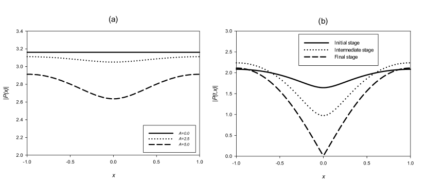
Figure 1: (a) The magnitude $\left|P\left(x\right)\right|$ of a steady-state $P\left(x\right)$ to (1) for $A$ with $\mu=\gamma_{N}=1,$ $\gamma_{L}=10,$ and $V\left(x\right)=\tanh(25x).$ (b) The time behavior of the magnitude $\left|P\left(t,x\right)\right|$ of a solution $P\left(t,x\right)$ to (1) with $\mu=\gamma_{N}=1,$ $\gamma_{L}=10,$ $A=10,$ and $V\left(x\right)=\tanh\left(25x\right)$ (the solid line: an initial stage; the dotted line: an intermediate stage; the dashed line: a final stage). The oscillation repeats these stages successively. $R=\left|P\right|$ in (a)-(b) satisfies $R^{\prime}\leq 0$ in $-1<x<0,$ and $R^{\prime}\geq 0$ in $0<x<1.$

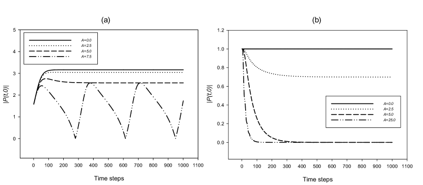
Figure 2: The evolution of the magnitude $|P(t,0)|$ of a solution $P(t,x)$ to (1) for $A$ with (a) $\mu=\gamma_{N}=1,$ $\gamma_{L}=10,$ $V\left(x\right)=\tanh\left(25x\right),$ and initial condition $P\left(0,x\right)=\frac{\left(\gamma_{L}/\gamma_{N}\right)^{1/2}}{2};$ (b) $\mu=\gamma_{N}=\gamma_{L}=1,$ $V\left(x\right)=\tanh\left(25x\right),\$and initial condition $P\left(0,x\right)=\left(\gamma_{L}/\gamma_{N}\right)^{1/2}.$ The difference of $\gamma_{L}$ between (a) and (b) shows the different long-time behavior for large $A$ ((a): nonlinear oscillation; (b): convergence to $0$).

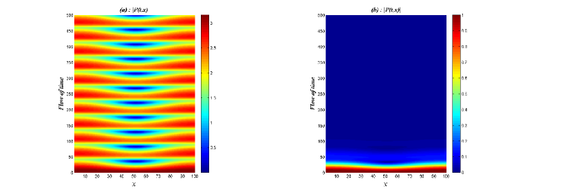
Figure 3: The evolution of the magnitude $\left|P\left(t,x\right)\right|$ (color bar) of a solution $P\left(t,x\right)$ to (1) for $A=10$ with (a) $\mu=\gamma_{N}=1,$ $\gamma_{L}=10,$ $V\left(x\right)=\tanh\left(25x\right),$ and initial condition $P\left(0,x\right)=\left(\gamma_{L}/\gamma_{N}\right)^{1/2};$ (b) $\mu=\gamma_{N}=\gamma_{L}=1,$ $V\left(x\right)=\tanh\left(25x\right),\$and initial condition $P\left(0,x\right)=\left(\gamma_{L}/\gamma_{N}\right)^{1/2}.$ The difference of $\gamma_{L}$ leads to the different long-time behavior for large $A$ ((a): nonlinear oscillation; (b): convergence to $0$).

II Numerical Verifications

We conduct numerical simulations for the pressure perturbation to support Theorem 1. We impose $V\left(x\right)=\tanh\left(25x\right)\$for numerical verifications. It is possible to confirm that the small shear leads to a steady-state in FIG. 1 (a). It is observed that the magnitude $|P(x)|=R(x)$ of all steady-states $P(x)=R(x)\exp(i\theta)$ in FIG. 1 (a) decreases in $x\in\left[-1,0\right]$ and increases in $x\in\left[0,1\right]$. This attribute in the profiles of steady-states is observed for a wide range of parameters of the complex GL equation. The shear acts as a force to keep down the magnitude $R(x)$ such that the force attains a maximum at the center $x=0$. Although we do not provide a figure of the evolution of $P\left(t,x\right)$ in $t,$ it was also possible to check that solutions converge to a steady-state for various initial conditions with a given small $A,$ so the long-time behavior of $P\left(t,x\right)$ for the weak shear is independent of initial conditions. These results are consistent with Theorem 1 $(a)$.

If the shear is large and GL parameters are suitable, then $|P\left(t,x\right)|$ oscillates nonlinearly and never converges to a steady-state. Indeed, FIG. 1 (b) displays the nonlinear oscillation. The solid line represents $|P\left(t,x\right)|$ when $|P\left(t,0\right)|$ peaks during the oscillation. After that, $|P\left(t,0\right)|$ drops to $0,$ so $|P\left(t,x\right)|$ reaches the dashed line finally. After the dashed line, $|P\left(t,x\right)|$ returns sharply to the solid line again. The dotted line shows an intermediate stage of the oscillation. $|P\left(t,x\right)|$ repeats this periodic oscillation without dissipation or blow-up. Moreover, many numerical results showed that $|P\left(t,x\right)|$ decreases in $x\in\left[-1,0\right]$ and increases in $x\in\left[0,1\right]$ for any time $t>0$ during the nonlinear oscillations. These oscillations are related to quasiperiodic ELM crash leconte2016ginzburg .

FIG. 2 (a) shows that the change of the time behavior of $|P\left(t,0\right)|$ for $A.$ $|P\left(t,0\right)|$ converges to a constant for small $A$ ($0.0,$ $2.5,$ and $5.0$ in FIG. 2 (a)), meaning that $|P\left(t,x\right)|$ converges to a steady-state. However, in the case of $A=7.5,$ it is shown that $|P\left(t,0\right)|$ oscillates without dissipation. Theorem 1 $(a)$ explains this bifurcation to the nonlinear oscillation from the steady-state because it is hard to expect steady-states except the zero solution for large $A$.

However, we emphasize that Theorem 1 $(b)$ provides a possibility that a solution may converge to $0$. Indeed, FIG. 2 (b) shows the convergence to the zero solution in $t$ with the change of $\gamma_{L}$ to $1$ from $10$ for large $A$ ($25.0$ in FIG. 2 (b)). Therefore, the long time behaviors between $\gamma_{L}=1$ and $\gamma_{L}=10$ are completely different for large $A$. FIG. 3 (a)-(b) represent the time behavior of $|P(t,x)|$ with $A=10$ for $\gamma_{L}=1\$and $10$ respectively. We also tested many cases by changing parameters and concluded that there are only two cases, that is, the nonlinear oscillation and the convergence to the zero solution.

It is important to understand the individual components of (2) to evaluate the relevance of our analysis to the experimental observed ELM dynamics. There are the dissipation term $\mu R^{\prime\prime}$ which has a role for flattening $R$, the linear growth term $\gamma_{L}R,$ nonlinear decay term $\gamma_{N}R^{3}$, and the term $\left|\theta^{\prime}\right|^{2}R$ related to the shear although the shear affects $\theta^{\prime}$ implicitly. Without the shear, the magnitude $R(t,x)$ and the phase $\theta^{\prime}(t,x)$ of the pressure perturbation $P\left(t,x\right)=R\left(t,x\right)\exp(i\theta\left(t,x\right))$ converge to $\left(\gamma_{L}/\gamma_{N}\right)^{1/2}$ and $0$ respectively as $t\rightarrow\infty$, but with nonzero $A>0,$ $\left|\theta^{\prime}\right|$ is nonzero, so the term $R\left|\theta^{\prime}\right|$ has a role to press $R$ perpetually. Besides, during the evolution, $\left|\theta^{\prime}\right|$ is increasing in $-1<x<0,$ decreasing in $0<x<1$, and maximum at $x=0$ at any time $t$ for suitable initial conditions. Consequently, the nonzero shear $\left(A>0\right)$ acts like a force to press $R$ such that it attains its maximum at the center $\left(x=0\right)$. This is why the profile of $R\left(t,x\right)$ is minimum at $x=0.$ For large shear ($A>>1$), the pressing force is dominant for $R>0$, so $R\left(t,0\right)$ approaches $0.$ During this procedure, the change of the slope of $R$ in a neighborhood of $x=0$ is so large that the term $\mu R^{\prime\prime}$ strongly affects the profile of $R$ as a restoration force with $\gamma_{L}R$. Therefore, the terms $\mu R^{\prime\prime}$ and $\gamma_{L}R$ acting as the restoring forces and the term $R\left|\theta^{\prime}\right|$ acting as the pressing force compete with each other. Here, we ignore $\gamma_{N}R^{3}$ due to $\gamma_{N}R^{3}<<\gamma_{L}R\$if $R<<1$. $\gamma_{N}R^{3}$ has a role to prevent the blowing-up of $R$. If $\gamma_{L}$ is weak, the restoring forces are insufficient to restore completely, so $R\left(t,x\right)$ converges to $0.$ Conversely, if $\gamma_{L}$ is strong, $R\left(t,x\right)$ has a tendency to restore completely, so $R\left(t,x\right)$ oscillates periodically.

The numerical results (in particular, FIG. 2 (a)) along with Theorem 1 provide a coherent picture on the ELM dynamics observed in the KSTAR tokamak lee2017solitary ; yun2011two ; mp3 . The quasi-steady ELM state lee2017solitary ; yun2011two may correspond to the situation where the shear flow is not sufficiently developed and below the bifurcation threshold. Furthermore, if the shear parameter $A$ is allowed to evolve in time, the abrupt transition from the quasi-steady state to the crash state lee2017solitary ; yun2011two may correspond to the situation where the shear flow gradually increases and exceeds the bifurcation threshold, which is plausible in the boundary of $H$-mode plasmas eb3 . This scenario would lead to quasi-periodic ELM oscillations (development of ELM and its crash), the common situation for the conventional $H$-mode plasmas. On the other hand, the suppression of the burst of ELM filaments by external magnetic perturbations mp3 may be explained by the reduction of the flow due to the magnetic perturbation (i.e., weakening of the parameter $A$) below the bifurcation threshold.

To conclude, the shear acts like a force to press the magnitude of the pressure perturbation, especially, strongly in a neighborhood of the center $x=0,$ so the sharp change around $x=0$ occurs if the shear is large. If $\gamma_{L}$ is large compared to $\mu>0$, the dissipation term $\mu R^{\prime\prime}$ and the linear growth term $\gamma_{L}R$ completely restore $R$ to the original state, so nonlinear oscillations occur. If the restoring effect by $\mu R^{\prime\prime}$ and $\gamma_{L}R$ is insufficient, $R$ converges to $0$ as $t\rightarrow\infty.$

III Conclusion

In summary, we obtained theoretical results to dramatically reduce the number of cases of the long time behavior of $P\left(t,x\right)$ in (1) which is a Ginzburg-Landau type model for ELMs in the one-dimensional case $\Omega=\left[-1,1\right]$. Besides, we also confirmed that these are consistent with the numerical results.

For the weak shear ($A<<1$), it is reasonable that solutions of (1) converge to a steady-state which is obtained in Theorem 1 $(a)$. For the strong shear ($A>>1$), it makes sense that solutions are to either converge to the zero solution or oscillate nonlinearly by Theorem 1 $(b)$. Besides, we confirmed that our results coincide with numerical results.

From these theoretical results, we believe that the model (1) for ELMs is quite reliable and useful for better understanding of the relaxation behavior which occurs in nature.

Appendix

In this appendix, we prove Theorem 1. For convenience, we set $\mu=\gamma_{L}=\gamma_{N}=1$ in (1). We will use the following function spaces:

$$L^{p}\left(\Omega\right) =\left\{f(x):\left\|f\right\|_{p}=\left\|f\right\|_{L^{p}}<\infty\right\},$$

$$H^{k}\left(\Omega\right) =\left\{f(x):\left\|f\right\|_{H^{k}}<\infty\right\},$$

$$H_{n}^{k}\left(\Omega\right) =\left\{f\left(x\right)\in H^{k}\left(\Omega\right):\partial_{x}f\left(\pm 1\right)=0\right\},$$

$$H_{0}^{k}\left(\Omega\right) =\left\{f\left(x\right)\in H^{k}\left(\Omega\right):f\left(\pm 1\right)=0\right\},$$

with $1\leq p\in\mathbb{R}$ and $0\leq k\in\mathbb{Z}$, where

$$\left\|f\right\|_{p}=\left(\int_{\Omega}|f(x)|^{p}dx\right)^{1/p},\ \left\|f\right\|_{H^{k}}=\left(\sum_{j=0}^{k}\left\|\frac{d^{j}f}{dx^{j}}\right\|_{2}^{2}\right)^{1/2}.$$

Finally, we use $C>0$ to denote a generic constant which is independent of parameters which we mainly consider in this paper.

Proof of Theorem 1 $(a)$

In the case of $A=0,$ we already know that $R\equiv 1\$and $\theta=c$ satisfy a solution of (2)-(3) for any constant $c.$ Without loss of generality, we assume that $\theta\left(0\right)=0.$ We consider the perturbation

$$R=1+r,\text{ }\theta=\theta+0,$$

so that we can express (2) as

$$\partial_{t}r-\partial_{x}^{2}r+2r =-3r^{2}-r^{3}-\left(1+r\right)w^{2},$$ (A.4)

$$\left(1+r\right)\partial_{t}w-\left(1+r\right)\partial_{x}w =2w\partial_{x}r-AV\left(x\right)\left(1+r\right),$$ (A.5)

where $w=\partial_{x}\theta.$

From now, we consider that both $r\$and $\theta$ are independent of $t.$ Then we can represent (A.5) as

$$R\left(x\right)^{2}w\left(x\right)=A\int_{-1}^{x}V\left(x\right)R\left(x\right)^{2}ds.$$ (A.6)

Due to $w\left(\pm 1\right)=0,$ (A.6) should satisfy the following compatibility condition for the Neumann boundary conditions as

$$\int_{-1}^{1}V\left(x\right)R\left(x\right)^{2}ds=0\text{ for }A\neq 0.$$ (A.7)

Note that (A.7) can be possible if $R\left(x\right)$ is even. Moreover, if $R\left(x\right)$ is even, $w\left(x\right)$ should be even. Indeed, we can derive $w\left(x\right)=w\left(-x\right)$ if $R\left(x\right)$ is even since

$$R^{2}\left(x\right)w\left(x\right) =\int_{-1}^{1}AV\left(s\right)R^{2}\left(s\right)ds-\int_{x}^{1}AV\left(s\right)R^{2}\left(s\right)ds=-\int_{x}^{1}AV\left(s\right)R^{2}\left(s\right)ds,$$

$$R^{2}\left(x\right)w\left(-x\right) =\int_{-1}^{-x}AV\left(s\right)R^{2}\left(s\right)ds=-\int_{x}^{1}AV\left(s\right)R^{2}\left(s\right)ds,$$

for any $x\in\Omega.$ Then we can also deduce that $\theta\left(-x\right)=-\theta\left(x\right)$ due to $\theta\left(0\right)=0.$ We will show the existence and uniqueness of $r$ and $w$ which satisfy (A.4)-(A.5) if $r$ and $w$ are sufficiently small in norms on $H^{2}\left(\Omega\right)$ and $H_{0}^{1}\left(\Omega\right)$ respectively.

We first consider the following linear problem.

$$-\partial_{x}^{2}r+2r =f,$$ (A.8)

$$-\partial_{x}w =g.$$ (A.9)

where $f$ and $g$ are given as $f\in L^{2}\left(\Omega\right)$ and $g\in L^{2}\left(\Omega\right)$ such that $\int_{-1}^{1}g\left(x\right)dx=0.$ Then there exist unique solutions $r\in H_{n}^{2}\left(\Omega\right)$ and $w\in H_{0}^{1}\left(\Omega\right)$ of (A.8)-(A.9) such that there is a constant $C>0$ such that

$$\left\|r\right\|_{H^{2}}\leq C\left\|f\right\|_{2}^{2},\text{ }\left\|w\right\|_{H^{1}}^{2}\leq C\left\|g\right\|_{2}^{2}.$$

Now we consider the following problem

$$-\Delta r+2r =f\left(q,\omega\right),$$ (A.10)

$$-\partial_{x}w =g\left(q,\omega\right),$$ (A.11)

with

$$f\left(q,\omega\right) =-3q^{2}-q^{3}-\left(1+q\right)\omega^{2},$$

$$g\left(q,\omega\right) =2\frac{\partial_{x}q\omega}{\left(1+q\right)}-AV\left(x\right)\left(1+q\right).$$

We assume that $q$ and $\omega$ belong to $B_{n,\varepsilon}^{2}$ and $B_{0,\varepsilon}^{1}$ respectively such that

$$B_{n,\varepsilon}^{2} =\left\{f\in H_{n}^{2}\left(\Omega\right):f\left(-x\right)=f\left(x\right),\text{ }\left\|f\right\|_{H^{2}}^{2}\leq\varepsilon^{2}\right\},$$

$$B_{0,\varepsilon}^{1} =\left\{f\in H_{0}^{1}\left(\Omega\right):f\left(-x\right)=f\left(x\right),\text{ }\left\|f\right\|_{H^{1}}^{2}\leq\varepsilon^{2}\right\},$$

for sufficiently small $\varepsilon<<1$. Then by the Sobolev embedding theorem (see Chapter 5 in pde ), we can easily show that

$$\left\|q\right\|_{\infty}^{2}\leq C\left\|q\right\|_{H^{2}}^{2}\leq C\varepsilon^{2},\left\|\nabla q\right\|_{\infty}^{2}\leq C\left\|q\right\|_{H^{2}}^{2}\leq C\varepsilon^{2},$$ (A.12)

for some constant $C>0.$ Therefore, for sufficiently small $\varepsilon<<1,$ $f\left(q,\omega\right)$ and $g\left(q,\omega\right)$ are well-defined in $L^{2}\left(\Omega\right).$ Moreover, we can also show that $f\left(q,\omega\right)\left(-x\right)=f\left(q,\omega\right)\left(x\right)$ and $g\left(q,\omega\right)\left(-x\right)=-g\left(q,\omega\right)\left(x\right)$ if $q$ and $\omega$ are even so that $\int_{-1}^{1}g\left(q,\omega\right)=0.$

Accordingly, we can define the following operator $S\left(q,\omega\right)=\left(r,w\right):B_{n,\varepsilon}^{2}\times B_{0,\varepsilon}^{1}\rightarrow H_{n}^{2}\left(\Omega\right)\times H_{n}^{1}\left(\Omega\right),$ where $r\$and $w$ are solutions of (A.10)-(A.11) such that they are both even. Besides, using (A.12), we can deduce that there is a $C>0$ such that

$$\left\|r\right\|_{H^{2}}^{2}+\left\|w\right\|_{H^{1}}^{2} \leq C\left(\left\|q\right\|_{H^{2}}^{4}+\left\|q\right\|_{H^{2}}^{6}+\left\|\omega\right\|_{H^{1}}^{4}\left(1+\left\|q\right\|_{H^{2}}^{2}\right)\right)$$

$$+C\frac{\left\|q\right\|_{H^{2}}^{2}\left\|\omega\right\|_{H^{1}}^{2}}{1-C\left\|q\right\|_{H^{2}}^{2}}+CA^{2}\left(1+\left\|q\right\|_{H^{2}}^{2}\right),$$

$$\leq\varepsilon^{2},$$

with sufficiently small $A<<1\$so that $S:B_{n,\varepsilon}^{2}\times B_{0,\varepsilon}^{1}\rightarrow B_{n,\varepsilon}^{2}\times B_{0,\varepsilon}^{1}$ for sufficiently small $\varepsilon$ and $A<<1.$ Using this fact and (A.12) again, we can estimate the differences $\widetilde{r}=r_{1}-r_{2},$ $\widetilde{w}=w_{1}-w_{2}$ for $\left(r_{1},w_{1}\right)=S\left(q_{1},\omega_{1}\right),$ $\left(r_{2},w_{2}\right)=S\left(q_{2},\omega_{2}\right)\in B_{n,\varepsilon}^{2}$ as

$$\left\|\widetilde{r}\right\|_{H^{2}}^{2}+\left\|\widetilde{w}\right\|_{H^{1}}^{2} \leq C\left(\varepsilon\left\|\widetilde{q}\right\|_{H^{2}}^{2}+\varepsilon\left\|\widetilde{\omega}\right\|_{H^{2}}^{2}+A^{2}\left\|\widetilde{q}\right\|\right)$$

$$\leq\frac{1}{2}\left(\left\|\widetilde{q}\right\|_{H^{2}}^{2}+\left\|\widetilde{\omega}\right\|_{H^{2}}^{2}\right),$$

for some $C>0$ and sufficiently small $\epsilon<<1.$ Then we can use the Banach fixed point theorem (see Chapter 9 in pde ) so that we can show the existence and uniqueness of solution $r$ and $w$ of (A.4)-(A.5).

Finally, the linearized equation of (A.4) on $r$ is

$$r_{t}-\Delta r+r\left|\nabla\theta\right|^{2}+2r=0.$$ (A.13)

Then multiplying $r$ to (A.13) and integrating in $x$ yield

$$\frac{d}{dt}\left\|r\right\|_{2}^{2}\leq 2\left\|r\right\|_{2}^{2}.$$ (A.14)

Therefore, we can conclude that $r$ is linearly stable due to (A.14). It is known that any nonconstant steady-state of (1) for $A=0$ is linearly unstable in a convex bounded domain jimbo1994stability . Moreover, the zero solution is unstable for $A=0.$ Let $\left\{P_{0,l},\lambda_{0,l}\right\}_{l\in S}$ be a set of linearly unstable steady-states $\left\{P_{0,l}\right\}_{l\in S}$ and the first eigenvalues $\left\{\lambda_{0,l}\right\}_{l\in S}$ such that $\left\{\lambda_{0,l}\right\}_{l\in S}\rightarrow 0$ of (1) for $A=0$ with an index set $S.$ Because of the uniform boundedness of $\left\{P_{0,l}\right\}_{l\in S}$ in $H^{1}\left(\Omega\right),$ we can choose a subsequence $\left\{P_{0,m\left(\sigma\right)},\lambda_{0,m\left(\sigma\right)}\right\}_{\sigma=1}^{\infty}$ of $\left\{P_{0,l},\lambda_{0,l}\right\}_{l\in S}$ such that $V\in H_{n}^{2}\left(\Omega\right)$ exists such that

$$P_{0,m\left(\sigma\right)} \rightarrow V\text{ weakly in }H_{n}^{1}\left(\Omega\right),$$

$$P_{0,m\left(\sigma\right)} \rightarrow V\text{ strongly in }L^{2}\left(\Omega\right),$$

as $\sigma\rightarrow 0$ (See Appendix D in pde ). Then $V$ is a steady-state, and it is not linearly unstable $\left(\lim_{\sigma\rightarrow\infty}\lambda_{0,m\left(\sigma\right)}=0\right)$, so $\left|V\right|\equiv 1,$ but it is a contradiction because of the definition of the stability. To conclude, there is some constant $C^{\ast}>0$ such that

$$0<C^{\ast}<\lambda_{0,l},$$

uniformly in $l.$

Therefore, we can complete the proof of Theorem 1 $\left(a\right).$

Proof of Theorem 1 $(b)$

We consider (2)-(3) without $t.$ Moreover, we use ${}^{\prime}=\frac{d}{dx}.$ Multiplying $R\left(x\right)\theta\left(x\right)$ to (3) and integrating in $x$ yield

$$\int_{-1}^{1}\left(R^{2}\theta\left(\theta^{\prime\prime}\right)+2R\left(R^{\prime}\right)\theta\left(\theta^{\prime}\right)\right)dx =-\int_{-1}^{1}R^{2}\left|\theta^{\prime}\right|^{2}dx\text{ by integration by parts}$$ (A.15)

$$=\int_{-1}^{1}AVR^{2}\theta dx\leq 0,$$

due to the Neumann boundary condition. Besides, multiplying $R$ to (3), integrating in $x,$ and applying (A.15), we can obtain

$$\left\|R^{\prime}\right\|_{2}^{2}+\int_{-1}^{1}R^{4}dx-\int_{-1}^{1}R^{2}\left(1+A\theta V\right)dx=0.$$ (A.16)

Now we prove that if $V$ satisfies the conditions in Theorem 1, then there is no $R\left(x\right)$ such that $R^{\prime}\left(x\right)\leq 0$ in $\left[-1,0\right]$ and $R\left(x\right)\geq 0$ except $R\left(x\right)\equiv 0$ for sufficiently large $A.$ By (A.16), it suffices to show

$$-\int_{-1}^{1}R^{2}\left(1+A\theta V\right)dx\geq 0,$$ (A.17)

for sufficiently large $A>0.$

We can generally assume that $R\left(x\right)>0$ for $-1\leq x\leq 1$ if $R\left(x\right)$ is nonconstant. Indeed, recall that we consider $0<R\left(x\right)$ such that $R^{\prime}\left(x\right)\leq 0$ in $-1\leq x<0$ and $R^{\prime}\left(x\right)\geq 0$ in $-1\leq x<0.$ If $R\left(-1\right)=R\left(1\right)>0$ initially, then $\theta^{\prime}\left(0\right)<0\$by (A.6). If $R\left(0\right)=0$ ($\min_{-1\leq x\leq 1}R\left(x\right)=R\left(0\right)$), then (3) leads to $R^{\prime}\left(0\right)\theta^{\prime}\left(0\right)=0.$ Due to $\theta^{\prime}\left(0\right)<0,$ $R^{\prime}\left(0\right)=0.$ With the help of ODE theory, however, then we can conclude that $R\left(x\right)\equiv 0$ for $-1\leq x\leq 1$ if $R\left(0\right)=R^{\prime}\left(0\right)=0.$

By (A.6) and the conditions for $V\left(x\right),$ $\theta^{\prime}$ is nonpositive. Besides, since $R\left(x\right)$ attains a minimum at $x=0$, so it leads to $\frac{R^{2}\left(x\right)}{R^{2}\left(0\right)}\geq 1$ for any $-1\leq x\leq 1$ and

$$\left|\theta^{\prime}\left(0\right)\right|\geq-A\int_{-1}^{0}V\left(s\right)ds,$$

by (A.6). Since $\theta^{\prime}\left(x\right)$ is continuous in $-1<x<0$ by (A.6), there is a region $\widetilde{x}<x<0$ such that

$$\left|\theta^{\prime}\left(x\right)\right|\geq-\frac{A}{2}\int_{-1}^{0}V\left(s\right)ds.$$

Notice that $\widetilde{x}$ is independent of $A.$ Therefore, we obtain

$$\theta\left(x\right) =-\int_{x}^{\widetilde{x}}\theta^{\prime}\left(y\right)dy-\int_{\widetilde{x}}^{0}\theta^{\prime}\left(y\right)dy\geq-\int_{\widetilde{x}}^{0}\theta^{\prime}\left(y\right)dy\geq\frac{A\widetilde{x}}{2}\int_{-1}^{0}V\left(s\right)ds,$$

for $-1\leq x\leq\widetilde{x}<0.$

Using (Proof of Theorem 1 $(b)$), we can compute (A.17) as

$$-\int_{-1}^{1}R^{2}\left(1+A\theta V\right)dx \geq-2\int_{-1}^{\widetilde{x}}R^{2}A\theta Vdx-2\int_{-1}^{0}R^{2}dx$$ (A.18)

$$\geq-A^{2}\widetilde{x}\left(\int_{-1}^{0}V\left(s\right)ds\right)\int_{-1}^{\widetilde{x}}R^{2}\left(x\right)V\left(x\right)dx$$

$$-2\int_{-1}^{\widetilde{x}}R^{2}dx-2\int_{\widetilde{x}}^{0}R^{2}dx.$$

Because $0<\left|V\left(x\right)\right|<C$ in $-1\leq x\leq\widetilde{x}<0$ for a constant $C>0,$ then it is easy to show

$$-\frac{A^{2}\widetilde{x}}{2}\left(\int_{-1}^{0}V\left(s\right)ds\right)\int_{-1}^{\widetilde{x}}R^{2}\left(x\right)V\left(x\right)dx>2\int_{-1}^{\widetilde{x}}R^{2}\left(x\right)dx,$$ (A.19)

if we choose large $A>0$. Besides, since

$$-\frac{A^{2}\widetilde{x}}{2}\left(\int_{-1}^{0}V\left(s\right)ds\right)\int_{-1}^{\widetilde{x}}R^{2}\left(x\right)V\left(x\right)dx \geq-\frac{A^{2}\widetilde{x}}{2}\left(\int_{-1}^{\widetilde{x}}V\left(s\right)ds\right)^{2}R^{2}\left(\widetilde{x}\right),$$

$$-2\widetilde{x}R^{2}\left(\widetilde{x}\right) \geq 2\int_{\widetilde{x}}^{0}R^{2}dx,$$

if we choose $A>0$ such that

$$-\frac{A^{2}\widetilde{x}}{2}\left(\int_{-1}^{\widetilde{x}}V\left(s\right)ds\right)^{2}R^{2}\left(\widetilde{x}\right)>-2\widetilde{x}R^{2}\left(\widetilde{x}\right),$$

then it is also obtainable that

$$-\frac{A^{2}\widetilde{x}}{2}\left(\int_{-1}^{0}V\left(s\right)ds\right)\int_{-1}^{\widetilde{x}}R^{2}\left(x\right)V\left(x\right)dx>2\int_{\widetilde{x}}^{0}R^{2}dx,$$ (A.20)

for large $A>0.$ Consequently, substituting (A.19) and (A.20) into (A.18), we can show (A.17).

Hence, Theorem 1 $(b)$ follows immediately.

References

- (1)
- (2) L. Mestel, Stellar magnetism. OUP Oxford, 2012, vol. 154.
- (3) J. D. Murray, Mathematical biology [electronic resource].: An introduction. Springer, 2002.
- (4) K. Burrell, “Effects of e b velocity shear and magnetic shear on turbulence and transport in magnetic confinement devices,” Physics of Plasmas, vol. 4, no. 5, pp. 1499–1518, 1997.
- (5) J. Cornelis, R. Sporken, G. Van Oost, and R. Weynants, “Predicting the radial electric field imposed by externally driven radial currents in tokamaks,” Nuclear fusion, vol. 34, no. 2, p. 171, 1994.
- (6) R. Groebner, “An emerging understanding of h-mode discharges in tokamaks,” Physics of Fluids B: Plasma Physics, vol. 5, no. 7, pp. 2343–2354, 1993.
- (7) R. Taylor, M. Brown, B. Fried, H. Grote, J. Liberati, G. Morales, P. Pribyl, D. Darrow, and M. Ono, “H-mode behavior induced by cross-field currents in a tokamak,” Physical review letters, vol. 63, no. 21, p. 2365, 1989.
- (8) F. Wagner, G. Becker, K. Behringer, D. Campbell, A. Eberhagen, W. Engelhardt, G. Fussmann, O. Gehre, J. Gernhardt, G. v. Gierke, et al., “Regime of improved confinement and high beta in neutral-beam-heated divertor discharges of the asdex tokamak,” Physical Review Letters, vol. 49, no. 19, p. 1408, 1982.
- (9) R. R. Weynants, G. Van Oost, G. Bertschinger, J. Boedo, P. Brys, T. Delvigne, K. Dippel, F. Durodie, H. Euringer, K. Finken, et al., “Confinement and profile changes induced by the presence of positive or negative radial electric fields in the edge of the textor tokamak,” Nuclear Fusion, vol. 32, no. 5, p. 837, 1992.
- (10) I. Krebs, M. Hoelzl, K. Lackner, and S. Günter, “Nonlinear excitation of low-n harmonics in reduced magnetohydrodynamic simulations of edge-localized modes,” Physics of Plasmas, vol. 20, no. 8, p. 082506, 2013.
- (11) J. Lee, G. Yun, W. Lee, M. Kim, M. Choi, J. Lee, M. Kim, H. Park, J. Bak, W. Ko, et al., “Solitary perturbations in the steep boundary of magnetized toroidal plasma,” Scientific Reports, vol. 7, p. 45075, 2017.
- (12) R. Wenninger, H. Zohm, J. Boom, A. Burckhart, M. Dunne, R. Dux, T. Eich, R. Fischer, C. Fuchs, M. Garcia-Munoz, et al., “Solitary magnetic perturbations at the elm onset,” Nuclear Fusion, vol. 52, no. 11, p. 114025, 2012.
- (13) P. Beyer, S. Benkadda, G. Fuhr-Chaudier, X. Garbet, P. Ghendrih, and Y. Sarazin, “Nonlinear dynamics of transport barrier relaxations in tokamak edge plasmas,” Physical review letters, vol. 94, no. 10, p. 105001, 2005.
- (14) S.-I. Itoh, K. Itoh, A. Fukuyama, and Y. Miura, “Edge localized mode activity as a limit cycle in tokamak plasmas,” Physical review letters, vol. 67, no. 18, p. 2485, 1991.
- (15) M. Leconte, Y. Jeon, and G. Yun, “Ginzburg-landau model in a finite shear-layer and onset of transport barrier nonlinear oscillations: A paradigm for typeiii elms,” Contributions to Plasma Physics, vol. 56, no. 6-8, pp. 736–741, 2016.
- (16) J. Lönnroth, V. Parail, G. Corrigan, D. Heading, G. Huysmans, A. Loarte, S. Saarelma, G. Saibene, S. Sharapov, J. Spence, et al., “Integrated predictive modelling of the effect of neutral gas puffing in elmy h-mode plasmas,” Plasma physics and controlled fusion, vol. 45, no. 9, p. 1689, 2003.
- (17) J. Connor, R. Hastie, H. Wilson, and R. Miller, “Magnetohydrodynamic stability of tokamak edge plasmas,” Physics of Plasmas, vol. 5, no. 7, pp. 2687–2700, 1998.
- (18) I. S. Aranson and L. Kramer, “The world of the complex ginzburg-landau equation,” Reviews of Modern Physics, vol. 74, no. 1, p. 99, 2002.
- (19) S. Jimbo and Y. Morita, “Stability of nonconstant steady-state solutions to a ginzburg–landau equation in higher space dimensions,” Nonlinear Analysis: Theory, Methods & Applications, vol. 22, no. 6, pp. 753–770, 1994.
- (20) F. Li and B. You, “Global attractors for the complex ginzburg–landau equation,” Journal of Mathematical Analysis and Applications, vol. 415, no. 1, pp. 14–24, 2014.
- (21) H. Lu, P. W. Bates, S. Lü, and M. Zhang, “Dynamics of the 3-d fractional complex ginzburg–landau equation,” Journal of Differential Equations, vol. 259, no. 10, pp. 5276–5301, 2015.
- (22) G. Yun, W. Lee, M. Choi, J. Lee, H. Park, B. Tobias, C. Domier, N. Luhmann Jr, A. Donné, J. Lee, et al., “Two-dimensional visualization of growth and burst of the edge-localized filaments in kstar h-mode plasmas,” Physical review letters, vol. 107, no. 4, p. 045004, 2011.
- (23) J. Lee, G. S. Yun, M. J. Choi, J.-M. Kwon, Y.-M. Jeon, W. Lee, N. C. Luhmann Jr, and H. K. Park, “Nonlinear interaction of edge-localized modes and turbulent eddies in toroidal plasma under n= 1 magnetic perturbation,” Physical Review Letters, vol. 117, no. 7, p. 075001, 2016.
- (24) L. Evans, Partial Differential Equations, ser. Graduate Studies in Mathematics. American Mathematical Society, Providence, 2010.