Robust Sparse Covariance Estimation by Thresholding Tyler’s M-Estimator

Abstract

Estimating a high-dimensional sparse covariance matrix from a limited number of samples is a fundamental problem in contemporary data analysis. Most proposals to date, however, are not robust to outliers or heavy tails. Towards bridging this gap, in this work we consider estimating a sparse shape matrix from $n$ samples following a possibly heavy tailed elliptical distribution. We propose estimators based on thresholding either Tyler’s M-estimator or its regularized variant. We derive bounds on the difference in spectral norm between our estimators and the shape matrix in the joint limit as the dimension $p$ and sample size $n$ tend to infinity with $p/n\to\gamma>0$. These bounds are minimax rate-optimal. Results on simulated data support our theoretical analysis.

1 Introduction

The covariance matrix $\bm{\Sigma}$ of a $p$-dimensional random variable $X$ is a central object in statistical data analysis. Given $n$ observations $\{\bm{x}_{i}\}_{i=1}^{n}$, accurately estimating this matrix is of great importance for many tasks including PCA, clustering and discriminant analysis (Anderson, 2003; Mardia, Kent and Bibby, 1979). The sample covariance matrix, which is the standard estimator for $\bm{\Sigma}$, is quite accurate when the random variable $X$ is sub-Gaussian and $p\ll n$.

In several contemporary applications, however, the number of samples $n$ and the dimension $p$ are comparable, and the data may be heavy tailed. To accurately estimate the covariance matrix when $n$ and $p$ are comparable, additional assumptions, such as its approximate sparsity are typically made. Over the past decade several sparse covariance matrix estimators were proposed and analyzed (Bickel and Levina, 2008; Cai and Liu, 2011; El Karoui, 2008; Lam and Fan, 2009; Rothman, Levina and Zhu, 2009). In addition, minimax lower bounds for estimating sparse covariance matrices in high-dimensional settings were established (Cai and Zhou, 2012a, b; Cai, Ren and Zhou, 2016).

With respect to heavy tailed data, a popular model which we consider in this work is the elliptical distribution (Cambanis, Huang and Simons, 1981; Fang, Kotz and Ng, 1990; Frahm, 2004; Kelker, 1970). An elliptical distribution is characterized by a $p\times p$ shape or scatter matrix $\bm{S}_{p}$, which equals a multiple of its population covariance matrix, when the latter exists. Since an elliptical distribution may be heavy tailed, the classical sample covariance may exhibit large variance and be a poor estimator of the population covariance (Falk, 2002). Moreover, the elliptical distribution might be so heavy tailed as to not even have finite second moments, in which case its population covariance does not exist. Yet due to the structure of the elliptical distribution, even with heavy tails it is nonetheless possible to accurately estimate its shape matrix. This is useful in various applications, since the shape matrix preserves the directional properties of the distribution, such as its principal components.

Following Huber’s pioneering work (Huber and Ronchetti, 2009), over the past decades several robust estimators of the covariance and shape matrix were proposed and theoretically studied, see Maronna (1976); Maronna and Yohai (2017); Kent and Tyler (1991); Dümbgen, Pauly and Schweizer (2015); Dümbgen, Nordhausen and Schuhmacher (2016) and references therein. For elliptical distributions, Tyler (1987a) proposed a robust M-estimator for the scatter matrix $\bm{S}_{p}$ and an iterative scheme to compute it. Tyler’s M-estimator has found widespread use in various applications involving heavy tailed data. However, as it is defined only for $p<n$, in recent years several regularized variants, applicable also for $p>n$ were proposed and analyzed (Abramovich and Spencer, 2007; Wiesel, 2012; Chen, Wiesel and Hero, 2011; Sun, Babu and Palomar, 2014; Pascal, Chitour and Quek, 2014; Ollila and Tyler, 2014). The spectral properties of Maronna’s M-estimators and specifically Tyler’s M-estimator and its regularized variants, in high dimensions as $n,p\to\infty$ with $p/n\to\gamma$ were studied by Dümbgen (1998); Couillet, Pascal and Silverstein (2014, 2015); Zhang, Cheng and Singer (2016); Couillet and McKay (2014); Couillet, Kammoun and Pascal (2016), among others. For a recent survey on Tyler’s M-estimator and its variants, see Wiesel and Zhang (2014).

In this paper we study the combination of heavy tailed data with a “large $p$ – large $n$” setting. As formulated in Section 2, we consider robust estimation of the shape matrix of an elliptical distribution, assuming it is approximately sparse. We address the following two challenges: (i) design a computationally efficient and statistically accurate estimator of the shape matrix $\bm{S}_{p}$, that is adaptive to its unknown sparsity parameters; (ii) provide theoretical guarantees on its accuracy, in the large $p$ large $n$ regime.

We make the following contributions. First, in Section 3 we propose simple and computationally efficient estimators for the sparse shape matrix of an elliptical distribution. These are based on thresholding either Tyler’s M-estimator (TME) or its regularized variant. Second, we provide theoretical guarantees on their accuracy in the limit $n,p\to\infty$ with $p/n\to\gamma$. Theorems 1 and 2 show that the estimator $\hat{\bm{E}}$ based on thresholding either TME for $\gamma<1$ or its regularized variant for any $\gamma\in(0,\infty)$, converges in spectral norm to a sparse shape matrix $\bm{S}_{p}$ at rate $\|\hat{\bm{E}}-\bm{S}_{p}\|=O_{P}((\log p/n)^{(1-q)/2})$, where $q$ is the sparsity parameter of $\bm{S}_{p}$. Estimating a sparse shape matrix under a heavy tailed elliptical distribution is thus possible with the same asymptotic error rate as estimating a sparse covariance matrix under sub-Gaussian distributions. Moreover, our estimators are rate optimal, as this rate coincides with the minimax rate for sparse covariance estimation with sub-Gaussian data (Cai and Zhou, 2012a).

Our proofs follow the approach of Bickel and Levina (2008), with required modifications given that we analyze Tyler’s M-estimators. Theorem 1, which provides guarantees for TME and is thus valid for $p<n$, is proven in Section 5. The proof is relatively simple and heavily relies on Zhang, Cheng and Singer (2016), who studied the spectral properties of Tyler’s M-estimator when $n,p\to\infty$. Theorem 2 provides guarantees on the thresholded regularized TME, and is thus applicable also for $p>n$. As detailed in Section 6, its proof is far more involved, and combines a careful analysis of the form of the regularized TME together with several results in random matrix theory. Section 7 presents simulation results that support our theoretical analysis. With an eye towards practitioners, given that regularization is common also when $p<n$, we focus on the regularized TME. With Gaussian data, our thresholded TME estimator is as accurate as thresholding the sample covariance. In contrast, in the presence of heavy tails it is far more accurate. We also illustrate its potential utility in handling outliers. In addition, our estimator is quite fast to compute in practice, requiring only few seconds on a standard PC, say for $p=n=1000$.

Our work is related to several recent papers, that also considered sparse shape or covariance matrix estimation with heavy tailed data. Han, Lu and Liu (2014) considered a pair-elliptical distribution, which is a different generalization of the classical elliptical distribution from the one we consider. They assumed moderate tails so the population covariance matrix exists, and proposed an estimator for it. They provided finite sample approximation bounds for their estimator, which depend on various properties of the distribution. For well-behaved elliptical distributions with an exactly sparse covariance matrix, their estimator is minimax rate optimal under the Frobenius norm. Soloveychik and Wiesel (2014) considered estimating a covariance matrix from a convex subset of all positive semidefinite matrices. They added a convex regularization term to the TME and solved the resulting optimization problem by a semidefinite program (SDP). They proved the existence of their estimator and its asymptotic consistency for fixed dimension $p$ and $n\to\infty$. However, their SDP-based method is computationally demanding even for moderate values of $n$ and $p$. Sun, Babu and Palomar (2016) considered a wider non-convex class of matrices, and derived an SDP-based algorithm with lower time complexity.

Chen, Gao and Ren (2018) considered an elliptical distribution, corrupted by an epsilon-contamination model. They proposed several estimators for the shape matrix of the elliptical distribution, based on a generalization of Tukey’s depth function. Under a notion of sparsity different from the one considered here, they proved their estimator is minimax rate optimal when $n,p\to\infty$ and $(\log p)/n\to 0$. However, from a practical perspective this depth function estimator has a significant limitation – it is intractable to compute. Balakrishnan et al. (2017) considered an epsilon-contamination model for a Gaussian distribution with sparse covariance matrix ${\bm{\Sigma}}$, such that $\|{\bm{\Sigma}-\bm{I}}\|_{0}\leq s$ for a fixed $s\geq 0$. They proposed a polynomial-time algorithm for robust covariance estimation under this model and established an upper bound on its error under Frobenius norm, assuming $n,p\to\infty$ and $(\log p)/n\to c\geq 0$. Our work in contrast provides a computationally efficient and rate optimal estimator for an approximately sparse shape matrix of a potentially heavy tailed elliptical distribution in the high dimensional setting $p,n\to\infty$ with $p/n\to\gamma$. Finally, Avella-Medina et al. (2018) developed rate optimal robust sparse covariance estimators for heavy tailed distributions via a different approach than the one presented here, based on various robust pilot estimators. Further discussion and directions for future research appear in Section 8.

2 Problem Setting

With precise definitions below, given $n$ i.i.d. observations from an elliptical distribution, the problem we study is how to estimate its $p\times p$ shape matrix $\bm{S}_{p}$. Of particular interest to us is the high-dimensional regime, where both $p,n$ are large and comparable. Following previous works, to be able to accurately estimate the shape matrix in this regime we assume that it is approximately sparse. For completeness, we first introduce some notation, briefly review the elliptical distribution and the class of approximately sparse shape matrices we consider.

Notation

We denote vectors by bold lowercase letters as in $\bm{v}$, and matrices by bold uppercase letters as in $\bm{A}$. For a vector $\bm{v}\in\mathbb{R}^{n}$, $\|\bm{v}\|$ is its Euclidean norm, $\|\bm{v}\|_{\infty}=\max_{i}|v_{i}|$, and $B_{R}(\bm{u})=\{\bm{v}\in\mathbb{R}^{n}\,|\,\|\bm{v}-\bm{u}\|_{\infty}\leq R\}$. The unit sphere in $\mathbb{R}^{p}$ is denoted $\mathbb{S}^{p-1}$. The identity matrix is $\bm{I}$ and $\bm{0}$ and $\bm{1}$ are the vectors of zeros and ones respectively, with dimensions clear from the context. For a matrix $\bm{A}=(a_{ij})$, $\|\bm{A}\|$ denotes its spectral norm, $\|\bm{A}\|_{F}$ its Frobenius norm, $\|\bm{A}\|_{\max}=\max_{i,j}|a_{ij}|$ and $\|\bm{A}\|_{\infty}=\max_{i}\sum_{j}|a_{ij}|$. We denote the set of $p\times p$ symmetric positive semidefinite and definite matrices by $S_{+}^{p}$ and $S_{++}^{p}$ respectively. We say that an event occurs with high probability (abbreviated w.h.p.), if its probability is at least $1-C\exp(-cp)$ for constants $c,C>0$ independent of $p$.

Elliptical Distribution and its Shape Matrix

A random vector $\bm{x}\in\mathbb{R}^{p}$ follows an elliptical distribution with location vector $\bm{\mu}$ if it has the form

$$\bm{x}=\bm{\mu}+u\bm{S}_{p}^{\frac{1}{2}}\bm{\xi}=\bm{\mu}+u\bm{z},$$ (1)

where $\bm{\xi}$ is drawn uniformly from $\mathbb{S}^{p-1}$, $\bm{S}_{p}\in S_{++}^{p}$, and $u$ is an arbitrary random or deterministic nonzero scalar, independent of $\bm{\xi}$.

In Eq. (1), $\bm{S}_{p}$ is not unique, as it can be arbitrarily scaled with $u$ absorbing the inverse scaling factor. Without loss of generality, we thus fix

$$\operatorname{tr}(\bm{S}_{p})=p,$$

and refer to $\bm{S}_{p}$ as the shape matrix. This normalization is natural in the sense that the mean variance of the $p$ coordinates of $\bm{z}$ is one. If the distribution is elliptical and the population covariance $\bm{\Sigma}$ exists, then $\bm{\Sigma}=c\bm{S}_{p}$ for some constant $c>0$, see for example Soloveychik and Wiesel (2014).

An important property of the elliptical distribution is that if $\bm{x}_{1},\bm{x}_{2}$ are independent random vectors from (1), then $\bm{x}_{1}-\bm{x}_{2}$ has an elliptical distribution with the same shape matrix $\bm{S}_{p}$ but with a zero location vector $\bm{\mu}=\bm{0}$. When the goal is to estimate the shape matrix $\bm{S}_{p}$, this allows to remove the typically unknown location vector by a symmetrization principle (Dümbgen, 1998). Specifically, all $\bm{x}_{i}-\bm{x}_{j}$ are elliptically distributed with location vector $\bm{\mu}=\bm{0}$, and one may estimate the shape matrix using all of these pairwise differences (Dümbgen, 1998; Sirkiä, Taskinen and Oja, 2007). As discussed by Nordhausen and Tyler (2015), such a procedure is beneficial also for non-elliptical distributions. The resulting $O(n^{2})$ pairs are, however, dependent which may complicate the analysis of the resulting estimator. For simplicity, we shall thus assume to have initially observed $2n$ i.i.d. samples $\tilde{\bm{x}}_{1},\ldots,\tilde{\bm{x}}_{2n}$ from model (1) and in what follows consider the $n$ differences $\bm{x}_{i}=\tilde{\bm{x}}_{2i}-\tilde{\bm{x}}_{2i-1}$ for $i=1,\ldots,n$ which form an i.i.d. sample from the elliptical distribution (1) with location vector $\bm{\mu}=\bm{0}$.

Approximate Sparsity of the Shape Matrix

Following Bickel and Levina (2008), we consider the following class of row/column approximately sparse shape matrices with fixed parameters $0\leq q\leq 1,M>0$ and $s_{p}>0$:

$$\mathcal{U}(q,s_{p},M)=\Big{\{}\bm{A}\in S_{++}^{p}:a_{ii}\leq M,\ \sum_{j=1}^{p}|a_{ij}|^{q}\leq s_{p},\ 1\leq i\leq p\Big{\}}.$$

Problem Statement

Let $\{\bm{x}_{i}\}_{i=1}^{n}$ be $n$ i.i.d. samples from the model (1) with location vector $\bm{\mu}=\bm{0}$ and a sparse shape matrix $\bm{S}_{p}\in\mathcal{U}(q,s_{p},M).$ We consider the following two problems: (i) Without explicit knowledge of $q,s_{p}$ and $M$, design a computationally efficient and statistically accurate estimator of the shape matrix $\bm{S}_{p}$; (ii) Provide theoretical guarantees on its accuracy, in the asymptotic limit as $p,n\to\infty$ with $p/n\to\gamma\in(0,\infty)$.

3 Sparse Shape Matrix Estimation

If the elliptical distribution is sub-Gaussian, then thresholding the sample covariance matrix, proposed by Bickel and Levina (2008) and El Karoui (2008), yields an accurate estimate of $\bm{S}_{p}$ up to a multiplicative scaling. As illustrated in Section 7, however, in the presence of heavy tails, the individual entries of the sample covariance matrix may be quite far from their population counterparts, and thresholding them may give a poor estimate of the shape matrix.

To handle heavy tails, we propose the following approach: compute Tyler’s M-estimator (TME) or its regularized variant, and threshold it. In Section 3.1 we review TME and its regularized variant. We prove that computing the latter is computationally efficient. Section 3.2 presents our proposed estimators. A theoretical analysis of their accuracy appears in Section 3.3.

3.1 TME and its Regularized Variant

TME, proposed by Tyler (1987a) for elliptical distributions with a known location vector, which w.l.o.g. is assumed to be $\bm{0}$, is a $p\times p$ matrix $\hat{\bm{\Sigma}}$ which satisfies

$$\frac{p}{n}\sum_{i=1}^{n}\frac{\bm{x}_{i}\bm{x}_{i}^{T}}{\bm{x}_{i}^{T}\hat{\bm{\Sigma}}^{-1}\bm{x}_{i}}=\hat{\bm{\Sigma}}.$$ (2)

Here, samples $\bm{x}_{i}$ lying at the origin are ignored as they provide no information on the scatter matrix, and $n$ is the number of samples not at the origin. As solutions to (2) can be multiplied by an arbitrary constant, Tyler (1987a) considered the normalization $\operatorname{tr}(\hat{\bm{\Sigma}})=p$, and suggested to solve Eq. (2) by the following iterations, starting from an arbitrary $\hat{\bm{\Sigma}}_{1}\in S_{++}^{p}$,

$$\hat{\bm{\Sigma}}_{k+1}=p\sum_{i=1}^{n}\frac{\bm{x}_{i}\bm{x}_{i}^{T}}{\bm{x}_{i}^{T}\hat{\bm{\Sigma}}_{k}^{-1}\bm{x}_{i}}\bigg{/}\operatorname{tr}\Big{(}\sum_{i=1}^{n}\frac{\bm{x}_{i}\bm{x}_{i}^{T}}{\bm{x}_{i}^{T}\hat{\bm{\Sigma}}_{k}^{-1}\bm{x}_{i}}\Big{)}.$$

Kent and Tyler (1988)[Theorems 1 and 2] showed that if any linear subspace in $\mathbb{R}^{p}$ of dimension $1\leq d\leq p-1$ contains less than $nd/p$ of the data samples, then there exists a unique solution to Eq. (2), and the above iterations converge to it. With $n$ i.i.d. observations from an elliptical distribution, no samples lie at the origin and this condition holds with probability $1$.

TME enjoys several important properties: First, it may equivalently be defined as the minimizer of the following cost function, over all positive definite matrices with the constraint $\operatorname{tr}(\bm{R})=p$,

$$L(\bm{R})=\frac{p}{n}\sum_{i=1}^{n}\log\left(\bm{x}_{i}^{T}\bm{R}^{-1}\bm{x}_{i}\right)+\log(\det(\bm{R})).$$ (3)

As the minimizer of Eq. (3), $\hat{\bm{\Sigma}}$ is thus the maximum likelihood estimator of the shape matrix of both the angular central Gaussian distribution (Tyler, 1987b) and of the generalized elliptical distribution (Frahm and Jaekel, 2010). Moreover, it is the “most robust” estimator of the shape matrix with fixed $p$ and $n\to\infty$ for data i.i.d. from a continuous elliptical distribution (Tyler, 1987a, Remark 3.1). TME outperforms the sample covariance in a variety of applications, including finance (Frahm and Jaekel, 2007), anomaly detection in wireless sensor networks (Chen, Wiesel and Hero, 2011), antenna array processing (Ollila and Koivunen, 2003) and radar detection (Ollila and Tyler, 2012).

As the TME does not exist when $p>n$, several regularized variants have been proposed and analyzed (Abramovich and Spencer, 2007; Chen, Wiesel and Hero, 2011; Wiesel, 2012; Pascal, Chitour and Quek, 2014; Sun, Babu and Palomar, 2014). Even when $p\leq n$, it is common to add small regularization to the TME. Following Sun, Babu and Palomar (2014), here we use a regularization parameter $\alpha>0$ and consider the following regularized TME $\hat{\bm{\Sigma}}(\alpha)$, defined as the solution of

$$\hat{\bm{\Sigma}}(\alpha)=\frac{1}{1+\alpha}\frac{p}{n}\sum_{i=1}^{n}\frac{\bm{x}_{i}\bm{x}_{i}^{T}}{\bm{x}_{i}^{T}\hat{\bm{\Sigma}}(\alpha)^{-1}\bm{x}_{i}}+\frac{\alpha}{1+\alpha}\bm{I}.$$ (4)

If $\alpha=0$, Eq. (4) reverts to Eq. (2). While regularization towards general target matrices is possible (Wiesel, 2012), here for simplicity we consider only regularization towards the identity. In contrast to the original TME formulated in Eq. (2), for which the solution can be multiplied by an arbitrary positive scalar, as proven by Pascal, Chitour and Quek (2014, Proposition III.1), any solution to Eq. (4) satisfies $\operatorname{tr}(\hat{\bm{\Sigma}}(\alpha)^{-1})=p$, regardless of the value of $\alpha$.

Sun, Babu and Palomar (2014, Theorem 11 and Proposition 13), derived a sufficient and necessary condition for existence of a unique positive definite matrix which solves Eq. (4). Again, ignoring samples at the origin, the condition is that any linear subspace in $\mathbb{R}^{p}$ of dimension $1\leq d\leq p-1$ contains less than $(1+\alpha)nd/p$ of the data samples. Since $\alpha>0$, this condition is weaker than for the original TME. In particular, with data i.i.d. from a continuous distribution, Eq. (4) has a unique solution for $\alpha>\max(0,p/n-1)$, see also Pascal, Chitour and Quek (2014, Theorem III.1). With $n$ i.i.d. samples from an elliptical distribution, these conditions hold with probability 1.

Sun, Babu and Palomar (2014, Proposition 18) further showed that starting from any positive definite initial guess, the following iterations

$$\hat{\bm{\Sigma}}_{k+1}(\alpha)=\frac{1}{1+\alpha}\frac{p}{n}\sum_{i=1}^{n}\frac{\bm{x}_{i}\bm{x}_{i}^{T}}{\bm{x}_{i}^{T}{{\hat{\bm{\Sigma}}_{k}}(\alpha)}^{\!-1}\bm{x}_{i}}+\frac{\alpha}{1+\alpha}\bm{I}$$ (5)

converge to the unique solution. Various properties of TME and its regularized variant, in the limit as $p,n\to\infty$ with $p/n\to\gamma$, were proven by Dümbgen (1998); Zhang, Cheng and Singer (2016); Couillet and McKay (2014); Couillet, Kammoun and Pascal (2016).

The following lemma, proven in the appendix, shows that if $\alpha$ is sufficiently large and $\bm{\Sigma}(\alpha)$ exists, then the iterations (5), starting from $\bm{\hat{\Sigma}}_{1}(\alpha)={\alpha}\bm{I}/{(1+\alpha)}$, have a uniform linear convergence rate already from the first iteration. To the best of our knowledge, this result is new and is of independent interest.

To state the lemma, let $e_{k}=\|\bm{\hat{\Sigma}}(\alpha)-\bm{\hat{\Sigma}}_{k}(\alpha)\|$ be the error after $k$ iterations, $\bm{\tilde{}}{\bm{X}}$ be the $p\times n$ matrix whose columns are $\{\bm{x}_{i}/\|\bm{x}_{i}\|\}_{i=1}^{n}$ and let

$$C(\bm{\tilde{}}{\bm{X}})=\frac{p}{n}\|\bm{\tilde{}}{\bm{X}}\tilde{\bm{X}}^{T}\|=\frac{p}{n}\left\|\sum_{i=1}^{n}\frac{\bm{x}_{i}\bm{x}_{i}^{T}}{\|\bm{x}_{i}\|^{2}}\right\|.$$

Note that for a given dataset, $C(\bm{\tilde{}}{\bm{X}})$ is fixed and can be computed a-priori.

Lemma 1.

Let $\{\bm{x}_{i}\}_{i=1}^{n}$ be a data set in $\mathbb{R}^{p}$ with constant $C(\bm{\tilde{}}{\bm{X}})$ and let $0<R<1$. Suppose that $\alpha>\max((3+R^{-1})C(\bm{\tilde{}}{\bm{X}})-1,0)$ and let $\hat{\bm{\Sigma}}(\alpha)$ be a solution of (4). Then, the iterations of Eq. (5), starting from $\bm{\hat{\Sigma}}_{1}(\alpha)=\frac{\alpha}{1+\alpha}\bm{I}$, uniformly and linearly converge to $\hat{\bm{\Sigma}}(\alpha)$ with the ratio $R$. That is,

$$e_{k+1}\leq Re_{k}\leq R^{k}e_{1},\ \text{for all }k\geq 1.$$ (6)

A straightforward calculation yields the bound $C(\bm{\tilde{}}{\bm{X}})\geq p/n$. Hence, the above assumptions on $\alpha$ imply that $\alpha>\max(0,p/n-1)$ and consequently guarantee the existence and uniqueness of $\bm{\hat{\Sigma}}(\alpha)$ in our setting.

Lemma 1 implies that calculating $\hat{\bm{\Sigma}}(\alpha)$ is computationally efficient, since for accuracy $\epsilon$ and convergence ratio $R$, at most $\lceil\log_{R^{-1}}(\epsilon^{-1})\rceil$ iterations are needed. If $n>p$ then at each iteration, the matrix inversion costs $O(p^{3})$ operations and the other operations are $O(n\,p^{2})$. For $n<p$ one may first perform an SVD of the data and compute the subspace $W=\text{Span}(\bm{x}_{i})$ whose dimension is at most $n$. Since for any $\bm{v}\bot W$, by definition $\hat{\bm{\Sigma}}(\alpha)\bm{v}=\alpha/(1+\alpha)\bm{v}$, it suffices to calculate $\hat{\bm{\Sigma}}(\alpha)$ restricted to the subspace $W$. Each iteration then costs at most $O(n^{3})$. Therefore, for sufficiently large $\alpha$, the total cost of computing $\hat{\bm{\Sigma}}(\alpha)$ within accuracy $\epsilon$ is $O(\log(\epsilon^{-1})(n+p)\min(n,p)^{2})$.

Our theoretical analysis below studies the regularized TME as $p,n\to\infty$ and $p/n\to\gamma\in(0,\infty)$, but with a fixed value of $\alpha$. The next lemma shows that for data sampled from an elliptical distribution, with high probability $C(\bm{\tilde{}}{\bm{X}})$ is bounded by a constant that depends on $\|\bm{S}_{p}\|$ and on the ratio $p/n$.

Lemma 2.

Let $\bm{x}_{1},\dots,\bm{x}_{n}$ be i.i.d. from Eq. (1) with $\bm{\mu}=\bm{0}$ and shape matrix $\bm{S}_{p}$. Then, with probability $>1-\exp(-cp)$, where $c=c(\|\bm{S}_{p}\|)>0$,

$$C(\bm{\tilde{}}{\bm{X}})\leq 2\|\bm{S}_{p}\|\Big{(}1+2\sqrt{p/n}\Big{)}^{2}.$$ (7)

3.2 TME-Based Thresholding Estimators

One possible approach to construct a sparse and robust estimator for the shape matrix is to add a suitable penalty to the original cost functional Eq. (3) of the TME. For various structural assumptions on the shape matrix, this approach was proposed by Soloveychik and Wiesel (2014) and by Sun, Babu and Palomar (2016).

For a sparsity inducing penalty, however, such an approach would in general lead to a non-convex and potentially difficult to optimize objective. As such, we instead opt for thresholding the (regularized) TME, which as we show in our paper, for sufficiently large regularization $\alpha$, can be computed efficiently in practical polynomial time.

For a matrix $\bm{A}=(a_{ij})$ and threshold $t>0$, define the hard-thresholding operator by

$$\tau_{t}(\bm{A})=({\bm{1}}(|a_{ij}|>t)a_{ij}).$$

For $n>p$, where the TME $\hat{\bm{\Sigma}}$ exists and by definition has unit trace, our proposed estimator for the shape matrix $\bm{S}_{p}$ takes the form

$$\hat{\bm{S}}_{p}=\tau_{t}\left({\hat{\bm{\Sigma}}}\right),\$$ (8)

where the threshold $t=t(p,n)$ is specified below. Similarly, for general $p,n$, our estimator based on the regularized TME is

$$\hat{\bm{S}}_{p}=\tau_{t}\left(p\frac{\hat{\bm{\Sigma}}(\alpha)-\tfrac{\alpha}{1+\alpha}\bm{I}}{\operatorname{tr}(\hat{\bm{\Sigma}}(\alpha)-\tfrac{\alpha}{1+\alpha}\bm{I})}\right).$$ (9)

Note that both $\hat{\bm{\Sigma}}$ in Eq. (8) and the argument matrix prior to thresholding in Eq. (9) have rank at most $\min(n,p)$.

3.3 Accuracy of the Thresholded TME

Theorems 1 and 2, proved in Sections 5 and 6, respectively, establish the asymptotic accuracy of Eqs. (8) and (9) as estimates of the shape matrix $\bm{S}_{p}$.

Theorem 1.

Consider a sequence $(n,p,\bm{S}_{p})$ where $n\to\infty,$ $p=p_{n}\to\infty$ with $p/n\to\gamma\in(0,1)$, and $\bm{S}_{p}\in\mathcal{U}(q,s_{p},M)$. For each triplet $(n,p,\bm{S}_{p})$, let $\hat{\bm{\Sigma}}$ be the TME of $n$ i.i.d. samples $\{\bm{x}_{i}\}_{i=1}^{n}\subset\mathbb{R}^{p}$ from the elliptical distribution (1). Then there exists a constant $M^{\prime}$ depending only on $\gamma$ such that for any fixed $M^{\prime\prime}>M^{\prime}$, the thresholded TME of Eq. (8) with threshold $t_{n}=M^{\prime\prime}\sqrt{{\log p}/{n}}$, approaches $\bm{S}_{p}$ in spectral norm at a rate

$$\Big{\|}\tau_{t_{n}}(p\bm{\hat{\Sigma}})-\bm{S}_{p}\Big{\|}=\mathcal{O}_{P}\bigg{(}s_{p}\cdot\left(\frac{\log p}{n}\right)^{(1-q)/2}\bigg{)}.$$

Theorem 2.

Consider a sequence $(n,p,\bm{S}_{p})$ as in Theorem 1, here with $p/n\to\gamma\in(0,\infty)$ and with the additional assumption that $\|\bm{S}_{p}\|\leq s_{\max}$. For ${\alpha}>\max(0,\gamma-1+s_{\max}(1+\sqrt{\gamma})^{2})$, let $\hat{\bm{\Sigma}}(\alpha)$ be the regularized TME of $n$ i.i.d. samples $\{\bm{x}_{i}\}_{i=1}^{n}\subset\mathbb{R}^{p}$ from the elliptical distribution (1). Then there exists an $M^{\prime}$ depending only on $\gamma$ and $\alpha$ such that for any fixed $M^{\prime\prime}>M^{\prime}$, the estimator of Eq. (9) with $t_{n}=M^{\prime\prime}\sqrt{{\log p}/{n}},$ converges in spectral norm to $\bm{S}_{p}$ at rate

$$\left\|\tau_{t_{n}}\left(p\frac{\left(\hat{\bm{\Sigma}}(\alpha)-\frac{\alpha}{1+\alpha}\bm{I}\right)}{\operatorname{tr}\left(\hat{\bm{\Sigma}}(\alpha)-\frac{\alpha}{1+\alpha}\bm{I}\right)}\right)-\bm{S}_{p}\right\|=\mathcal{O}_{P}\left(s_{p}\left(\frac{\log p}{n}\right)^{(1-q)/2}\right).$$

Several remarks regarding Theorem 2 are in place.

Remark 1.

As noted by Bickel and Levina (2008, p. 2580), if $\bm{S}_{p}\in\mathcal{U}(q,s_{p},M)$ then $\|\bm{S}_{p}\|\leq M^{1-q}s_{p}$ which may grow with $p$. Since we analyze the regularized TME with a fixed value of $\alpha$, we explicitly require that $\|\bm{S}_{p}\|\leq s_{\max}$ independent of $p$. If the sequence of matrices $\bm{S}_{p}$ has a norm that grows to infinity with $p$, then the regularization $\alpha$ should also grow to infinity with $p$, such that $\alpha>c\|\bm{S}_{p}\|$ for some constant $c>0$. We believe an analogue of Theorem 2 should hold in this case, but this requires a careful analysis beyond the scope of this paper.

Remark 2.

The convergence rate in Theorems 1 and 2 coincides with the minimax optimal rate for sparse covariance estimation with sub-Gaussian data, derived by Cai and Zhou (2012a). Since the Gaussian distribution is a particular case of an elliptical distribution, our estimators are thus minimax rate optimal. Furthermore, in light of Lemmas 1 and 2, computing the regularized TME and subsequently thresholding it, is computationally efficient.

Remark 3.

One use of regularized variants of Tyler’s M-estimator is to provide an accurate estimate of the shape matrix when $p>n$. With this goal in mind, choosing the precise value of the regularization constant is crucial (Chen, Wiesel and Hero, 2011; Couillet and McKay, 2014). Setting the regularization parameter is also important to maximize the asymptotic detection probability in various signal processing applications (Kammoun et al., 2018). In contrast, in our case, as we remove the regularization $\alpha/(1+\alpha)\bm{I}$ prior to thresholding, at least asymptotically, the precise value of the regularization parameter is unimportant, provided it is sufficiently large. This is also evident in the simulations described in Section 7. From a practical perspective, we thus suggest to use a value of $\alpha$ as described in Lemma 1, with say $R=1/2$, which is not only sufficient for existence but also guarantees fast convergence of the iterations to compute the regularized TME.

4 Preliminaries

In proving Theorems 1 and 2, we shall make frequent use of the following auxiliary lemmas. The first is a simple inequality. Let $A,B$ be non-negative random variables. Then for any $c>0$ and $\lambda>0$,

$$\Pr(AB>c)\leq\Pr(A>\lambda c)+\Pr(B>1/\lambda).$$ (10)

Next, is the following well known result, which shows that TME and regularized TME are unable to distinguish an elliptical distribution from a Gaussian one. Its proof (omitted) follows directly from the fact that (regularized) TME for data $\bm{x}_{i}$ is identical to that of data $t_{i}\bm{x}_{i}$, where $t_{i}$ are arbitrary positive real valued numbers.

Lemma 3.

TME or regularized TME with $\alpha>\max(0,p/n-1)$ under an elliptical distribution with shape matrix $\bm{S}_{p}$ has the same distribution as under a Gaussian distribution with covariance $\bm{S}_{p}$.

The following two results from random matrix theory will also be of use. The first is a non-asymptotic bound on the spectral norm of a Wishart matrix, and the second on the concentration of quadratic forms. See for example (Davidson and Szarek, 2001)[Theorem 2.13] and (Rudelson and Vershynin, 2013)[Theorem 1.1].

Lemma 4.

Let $\{\bm{\xi}_{i}\}_{i=1}^{n}\subset\mathbb{R}^{p}$ be i.i.d. $N(0,\bm{I})$, and let $\bm{T}_{n}=\frac{1}{n}\sum_{i}\bm{\xi}_{i}\bm{\xi}_{i}^{T}$. Then, $\mathbb{E}[\|\bm{T}_{n}\|]\leq(1+\sqrt{p/n})^{2}$ and

$$\Pr\left(\|\bm{T}_{n}\|>\bigg{(}1+\sqrt{p/n}+t\bigg{)}^{2}\right)\leq\exp\left(-nt^{2}/2\right).$$

Lemma 5.

Let $\bm{A}\in\mathbb{R}^{p\times p}$ and $\bm{\xi}\sim N(\bm{0},\bm{I})$. Then, there exist absolute constants $c_{1},c_{2}>0$ such that for all $\epsilon>0$,

$$\Pr\left(\left|\bm{\xi}^{T}\bm{A}\bm{\xi}-{\operatorname{tr}}\left(\bm{A}\right)\right|>\epsilon\right)\leq 2\exp\left(-c_{1}\min\left\{\frac{c_{2}^{2}\epsilon^{2}}{\left\|\bm{A}\right\|_{F}^{2}},\frac{c_{2}\epsilon}{\left\|\bm{A}\right\|}\right\}\right).$$

Finally, the following auxiliary lemma, proved in Appendix A.2, is a slight modification of a result by Bickel and Levina (2008, p. 2583).

Lemma 6.

Assume $\bm{B}\in\mathcal{U}(q,s_{p},M).$ Let $\bm{A}$ be a matrix such that

$$\big{\|}\bm{A}-\bm{B}\big{\|}_{\max}\leq C_{1}\sqrt{\log p/n},$$

for some $C_{1}>0$. Suppose we threshold $\bm{A}$ at level $t=K\sqrt{\log p/n}$, with $K>C_{1}$. Then, there exists a constant $C_{2}=C_{2}(C_{1},K,q)<\infty$ such that

$$\big{\|}\tau_{t}(\bm{A})-\bm{B}\big{\|}\leq C_{2}s_{p}(\log p/n)^{(1-q)/2}.$$

5 Proof of Theorem 1

The proof consists of three main steps: (i) reducing to a bound on $\|\bm{\hat{\Sigma}}-\bm{\hat{S}}\|_{\max}$; (ii) expressing $\hat{\bm{\Sigma}}$ as a weighted covariance matrix whose coefficients are all uniformly close to a constant, with high probability; and (iii) bounding $\|\bm{\hat{\Sigma}}-\bm{\hat{S}}\|_{\max}$.

5.1 Step 1: Reduction from $\|\tau_{t_{n}}(\bm{\hat{\Sigma}})-\bm{S}_{p}\|$ to $\|\bm{\hat{\Sigma}}-\bm{\hat{S}}\|_{\max}$

By Lemma 6, it suffices to prove that $\|\bm{\hat{\Sigma}}-\bm{S}_{p}\|_{\max}=\mathcal{O}_{P}(\sqrt{\log p/n})$. Let $\hat{\bm{S}}$ be the sample covariance of $\{\bm{x}_{i}\}_{i=1}^{n}$. By the triangle inequality,

$$\|\hat{\bm{\Sigma}}-\bm{S}_{p}\|_{\max}\leq\|\hat{\bm{\Sigma}}-\bm{\hat{S}}\|_{\max}+\|\bm{\hat{S}}-\bm{S}_{p}\|_{\max}.$$

In light of Lemma 3, we may assume that $\bm{x}_{i}$ are all i.i.d. $N(\bm{0},\bm{S}_{p})$ . Since the proof of Theorem 1 of Bickel and Levina (2008) shows that

$$\|\bm{\hat{S}}-\bm{S}_{p}\|_{\max}=\mathcal{O}_{P}\left(\sqrt{\log p/n}\right)$$

it thus suffices to show that

$$\|\bm{\hat{\Sigma}}-\bm{\hat{S}}\|_{\max}=\mathcal{O}_{P}\left(\sqrt{\log p/n}\right).$$ (11)

5.2 Step 2: The weights of TME

By Zhang, Cheng and Singer (2016, Lemma 2.1), TME has an equivalent definition as a weighted covariance matrix,

$$\bm{\hat{\Sigma}}=p\sum_{i=1}^{n}w_{i}\bm{x}_{i}\bm{x}_{i}^{T}\Big{/}\operatorname{tr}\Big{(}\sum_{i=1}^{n}w_{i}\bm{x}_{i}\bm{x}_{i}^{T}\Big{)},$$

where the weights $w_{i}$ are the unique solution of

$$\underset{{w_{i}>0,\sum w_{i}=1}}{\arg\min}-\sum_{i=1}^{n}\ln w_{i}+\frac{n}{p}\ln\det\bigg{(}\sum_{i=1}^{n}w_{i}\bm{x}_{i}\bm{x}_{i}^{T}\bigg{)}.$$ (12)

This characterization is important because of the following result:

Lemma 7.

Consider a sequence $(n,p,\bm{S}_{p})$ where $n,p\to\infty$ with $p/n\to\gamma\in(0,1)$, and $\bm{S}_{p}\in S_{++}^{p}$. For every triplet $(n,p,\bm{S}_{p})$, let $\bm{x}_{i}\overset{iid}{\sim}N(\bm{0},\bm{S}_{p})$ and let $\{w_{i}\}_{i=1}^{n}$ be the corresponding weights of Eq. (12). Then there exist positive constants $C,c$ and $c^{\prime}$ depending only on $\gamma$ such that for any $0<\epsilon<c^{\prime}$, and sufficiently large $n$,

$${\rm{Pr}}\left[\max_{i}|nw_{i}-1|\geq\epsilon\right]\leq Cne^{-c\epsilon^{2}n}.$$ (13)

The case $\bm{S}_{p}=\bm{I}$ was proved by Zhang, Cheng and Singer (2016, Lemma 2.2). Its generalization to an arbitrary $\bm{S}_{p}\in S_{++}^{p}$ is proved in Appendix A.3.

5.3 Step 3: Bounding $\|\hat{\bm{\Sigma}}-\hat{\bm{S}}\|_{\max}$

The proof of Theorem 1 concludes by applying the following lemma which establishes Eq. (11). Its proof is in Appendix A.4.

Lemma 8.

Let $\hat{\bm{\Sigma}}$ and $\hat{\bm{S}}$ be the TME and the sample covariance matrix of $\bm{x}_{1},\dots,\bm{x}_{n}$ i.i.d. from $N(\bm{0},\bm{S}_{p})$, where $\bm{S}_{p}\in\mathcal{U}(q,s_{p},M)$ with $tr(\bm{S}_{p})=p$. Assume that $p,n\to\infty$, with $p/n\to\gamma\in(0,1)$. Then there exist positive constants $C,c$ and $c^{\prime}$ that depend only on $\gamma$, such that for all $\epsilon\in(0,c^{\prime})$ and $n$ sufficiently large

$${\rm{Pr}}\left(\|\bm{\hat{\Sigma}}-\bm{\hat{S}}\|_{\max}\geq\epsilon\right)\leq Cne^{-c\epsilon^{2}n}.$$

6 Proof of Theorem 2

We first introduce and prove a slightly modified version of Theorem 2. We then show how Theorem 2 follows from it. The modified theorem uses the following proposition, proved in Appendix A.5.

Proposition 1.

Let $\bm{y},\bm{\xi}_{1},\dots,\bm{\xi}_{n-1}\in\mathbb{R}^{p}$ be i.i.d. $N(\bm{0},\bm{I})$ and denote

$$Q=Q(r)=\frac{1}{p}\bm{y}^{T}\left(\frac{1}{n}\sum_{j=1}^{n-1}\bm{\xi}_{j}\bm{\xi}_{j}^{T}+\alpha\frac{n}{p}\frac{1}{r}\bm{S}_{p}^{-1}\right)^{-1}\bm{y},$$

where $\bm{S}_{p}\in\mathcal{U}(q,s_{p},M)$ with $\|\bm{S}_{p}\|\leq s_{\max}$. Assume that $\alpha>\max(0,p/n-1+s_{\max}(1+\sqrt{p/n})^{2})$, and define

$$r_{\min}=\frac{n}{p}\frac{\alpha}{1+\alpha-p/n},\quad r_{\max}=\frac{n}{p}\frac{\alpha}{1+\alpha-p/n-s_{\max}(1+\sqrt{p/n})^{2}}.$$

Then, there exists a unique $r=r(p,n,\alpha,\bm{S}_{p})\in[r_{\min},r_{\max}]$, such that

$$\mathbb{E}[Q(r)]=\frac{1}{1+\alpha-p/n},$$ (14)

where the expectation is over $\bm{y}$ and $\bm{\xi}_{1},\ldots,\bm{\xi}_{n-1}$.

6.1 A reformulation of the main result

We now introduce the modified theorem.

Theorem 3.

Consider the same setting as in Theorem 2. Then there exists an $M^{\prime}$ depending only on $\gamma$ and $\alpha$ such that for any fixed $M^{\prime\prime}>M^{\prime}$, the estimator $\tau_{t_{n}}(\hat{\bm{\Sigma}}(\alpha)-{\alpha}\bm{I}/(1+\alpha))$ with $t_{n}=M^{\prime\prime}\sqrt{\frac{\log p}{n}},$ converges in spectral norm to a multiple of $\bm{S}_{p}$,

$$\left\|\tau_{t_{n}}\left(\hat{\bm{\Sigma}}(\alpha)-\frac{\alpha}{1+\alpha}\bm{I}\right)-\frac{p}{n}\frac{r}{1+\alpha}\bm{S}_{p}\right\|=\mathcal{O}_{P}\left(s_{p}\left(\frac{\log p}{n}\right)^{(1-q)/2}\right),$$

where the scalar $r=r(p,n,\alpha,\bm{S}_{p})$ is specified in Proposition 1.

6.2 Proof of Theorem 3

By Lemma 3, we may assume $\bm{x}_{i}\overset{iid}{\sim}N(\bm{0},\bm{S}_{p})$. Following the argument in Section 5.1, combining Lemma 6 with the fact that by Proposition 1, $r<r_{\max}$, it suffices to show that

$$\left\|\left(\hat{\bm{\Sigma}}(\alpha)-\frac{\alpha}{1+\alpha}\bm{I}\right)-\frac{p}{n}\frac{r}{1+\alpha}\bm{\hat{S}}\right\|_{\max}=\mathcal{O}_{P}\left(\sqrt{\log p/n}\right).$$ (15)

Our proof proceeds as follows: First, we express $\hat{\bm{\Sigma}}(\alpha)$ as the sum of $\frac{\alpha}{1+\alpha}{\bm{I}}$ and weighted $\bm{x}_{i}\bm{x}_{i}^{T}$ terms, where the weights are the root of some equation. Next, we show that this root is concentrated near the vector $r{\bm{1}}/n$, with $r$ specified in Proposition 1. Finally, we establish Eq. (15).

Following the definition of the regularized TME, we write $\hat{\bm{\Sigma}}(\alpha)$ as

$$\hat{\bm{\Sigma}}(\alpha)=\frac{1}{1+\alpha}\frac{p}{n}\sum_{i=1}^{n}w_{i}\bm{x}_{i}\bm{x}_{i}^{T}+\frac{\alpha}{1+\alpha}\bm{I},$$ (16)

where the weight vector $\bm{w}=(w_{1},\dots,w_{n})^{T}$ satisfies

$$w_{i}=\frac{1}{\bm{x}_{i}^{T}\hat{\bm{\Sigma}}(\alpha)^{-1}\bm{x}_{i}}=\frac{1}{\bm{x}_{i}^{T}\left(\frac{1}{1+\alpha}\frac{p}{n}\sum_{j=1}^{n}w_{j}\bm{x}_{j}\bm{x}_{j}^{T}+\frac{\alpha}{1+\alpha}\bm{I}\right)^{-1}\bm{x}_{i}}.$$ (17)

By Sun, Babu and Palomar (2014)[Theorem 11], $\hat{\bm{\Sigma}}(\alpha)$ is unique.

Next, consider the function $g:\mathbb{R}^{n}\to\mathbb{R}^{n}$ whose $n$ components are

$$g(\bm{v})_{i}=v_{i}-\frac{1}{\bm{x}_{i}^{T}\left(\frac{1}{1+\alpha}\frac{p}{n}\sum_{k=1}^{n}v_{k}\bm{x}_{k}\bm{x}_{k}^{T}+\frac{\alpha}{1+\alpha}n\bm{I}\right)^{-1}\bm{x}_{i}}.$$ (18)

Comparing Eq. (18) to Eq. (17), the $n$ non-linear equations $g(\bm{v})=\bm{0}$ have a unique solution, which is thus $n\bm{w}$. The next three lemmas state properties of $g$ used to prove that as $p,n\to\infty$, with $p/n\to\gamma$, this root concentrates around $\bm{u}=r\bm{1}$, with $r$ given in Proposition 1. The lemmas, proven in Appendices A.6–A.8, assume the setting of Theorem 3, and their generic constants depend only on $\gamma,\alpha$ and $s_{\max}$. Our analysis of the weights $w_{i}$ follows the pioneering works of Couillet, Pascal and Silverstein (2014, 2015), who proved that the weights in Maronna’s M-estimators converge to suitable constants, and Zhang, Cheng and Singer (2016), who derived concentration results for the weights of Tyler’s M-estimator as $p,n\to\infty$ with $p/n\to\gamma<1$.

Lemma 9.

There exist $C,c>0$ such that for any $\epsilon\in(0,1)$

$${\rm{Pr}}\left(\left\|g(\bm{u})\right\|_{\infty}>\epsilon\right)<Cpe^{-cp\epsilon^{2}}.$$

Lemma 10.

There exist $c^{\prime},c_{L},C,c>0$ such that

$$\Pr\left(\exists{\bm{v}}\in B_{c^{\prime}}(\bm{u}),\left\|\nabla g\left(\bm{v}\right)-\nabla g\left(\bm{u}\right)\right\|_{\max}>c_{L}\|\bm{v}-\bm{u}\|_{\infty}\right)<Cp^{2}e^{-cp}.$$

Lemma 11.

There exist $c_{H},C,c>0$ such that

$${\rm{Pr}}\left(\left\|\left(\nabla g\left(\bm{u}\right)\right)^{-1}\right\|_{\infty}>c_{H}\right)<Cpe^{-cp}.$$ (19)

Lemmas 9 and 10 show that w.h.p. $g(\bm{u})$ is small and $\nabla g$ is Lipschitz near $\bm{u}$. These two properties are consistent with the root of $g$ being close to $\bm{u}$. To rigorously prove this, following Zhang, Cheng and Singer (2016), we consider the function $f(\bm{v})=\left(\nabla g(\bm{u})\right)^{-1}g(\bm{v})$. Lemma 11 shows that the matrix $(\nabla g(\bm{u}))^{-1}$ is w.h.p. not extremely large. Finally, the following lemma combines these properties of $g$ to infer that its root is close to $\bm{u}$.

Lemma 12.

Let $f:\mathbb{R}^{n}\to\mathbb{R}^{n}$, $\bm{u}\in\mathbb{R}^{n}$ and $C>0$. Assume that

1. $\nabla f(\bm{u})=\bm{I}$;

2. $\|\nabla f(\bm{v})-\nabla f(\bm{u})\|_{\max}\leq C\|\bm{v}-\bm{u}\|_{\infty}$ for all $\|\bm{v}-\bm{u}\|_{\infty}\leq 3\|f(\bm{u})\|_{\infty}$;

3. $\|f(\bm{u})\|_{\infty}<\min\{1/(9C),1/3\}$.

Then there exists a $\bm{\tilde{v}}\in\mathbb{R}^{n}$ such that $f(\bm{\tilde{v}})=\bm{0}$ and $\|\bm{\tilde{v}}-\bm{u}\|_{\infty}<3\|f(\bm{u})\|_{\infty}$.

Lemma 12 is slightly stronger than Lemma 3.1 of Zhang, Cheng and Singer (2016), as it has a weaker requirement that the Lipschitz condition in Lemma 12 holds in a smaller ball $\|\bm{v}-\bm{u}\|_{\infty}\leq 3\|f(\bm{u})\|_{\infty}$, instead of the original requirement $\|\bm{v}-\bm{u}\|_{\infty}<1$ in their Lemma 3.1. A careful inspection shows that their original proof is still valid under this weaker assumption.

To apply Lemma 12 to $f(\bm{v})=\left(\nabla g(\bm{u})\right)^{-1}g(\bm{v})$, we verify that the three conditions of the lemma hold with high probability. The first condition is trivially satisfied. For the other two conditions, by Lemmas 9 and 11, w.h.p.

$$\|f(\bm{u})\|_{\infty}\leq\|(\nabla g(\bm{u}))^{-1}\|_{\infty}\cdot\|g(\bm{u})\|_{\infty}\leq c_{H}\epsilon.$$

Similarly, by Lemmas 10 and 11, for all $\|\bm{v}-\bm{u}\|_{\infty}\leq c^{\prime}$, w.h.p.

$$\|\nabla f(\bm{v})-\nabla f(\bm{u})\|_{\max}\leq\|(\nabla g(\bm{u}))^{-1}\|_{\infty}\cdot\|\,\nabla g(\bm{v})-\nabla g(\bm{u})\|_{\max}\leq c_{H}c_{L}\|\bm{v}-\bm{u}\|_{\infty}.$$

Since for sufficiently small $\epsilon$, $c_{H}\epsilon<\min\{1/(9c_{L}c_{H}),1/3\}$, both the second and third conditions of Lemma 12 are thus satisfied with constant $C=c_{L}c_{H}$.

To conclude, with probability at least $1-Cp^{2}e^{-cp\epsilon^{2}}$all three conditions of Lemma 12 hold, so there exists $\tilde{\bm{v}}\in\mathbb{R}^{n}$ such that $f(\tilde{\bm{v}})=\bm{0}$ and $\|\tilde{\bm{v}}-\bm{u}\|_{\infty}\leq 3\|f(\bm{u})\|_{\infty}<3c_{H}\epsilon$. Since $n\bm{w}$ is the unique root of $g(\bm{v})$ and also of $f(\bm{v})$,

$$\Pr\left(\|n\bm{w}-r\bm{1}\|_{\infty}>3c_{H}\epsilon\right)<Cp^{2}e^{-cp\epsilon^{2}}.$$ (20)

Next, we use Eq. (20) to bound the LHS of Eq. (15). First, by Eq. (16),

$$\left\|\left(\hat{\bm{\Sigma}}(\alpha)-\tfrac{\alpha}{1+\alpha}\bm{I}\right)-\tfrac{1}{1+\alpha}\tfrac{p}{n}r\hat{\bm{S}}\right\|_{\max} = \tfrac{1}{1+\alpha}\tfrac{p}{n}\left\|\sum_{i=1}^{n}w_{i}\bm{x}_{i}\bm{x}_{i}^{T}-r\tfrac{1}{n}\sum_{i=1}^{n}\bm{x}_{i}\bm{x}_{i}^{T}\right\|_{\max}$$

$$\leq \tfrac{1}{1+\alpha}\tfrac{p}{n}\left\|n\bm{w}-r\bm{1}\right\|_{\infty}\left\|\tfrac{1}{n}\sum_{i=1}^{n}\bm{x}_{i}\bm{x}_{i}^{T}\right\|_{\max}.$$

Using this inequality and Eq. (10) with $\lambda=1/[s_{\max}(1+2\sqrt{\gamma})^{2}]$,

$$\Pr\left(\left\|(\hat{\bm{\Sigma}}(\alpha)-\tfrac{\alpha}{1+\alpha}\bm{I})-\tfrac{1}{1+\alpha}\tfrac{p}{n}r\hat{\bm{S}}\right\|>\epsilon\right)\leq\Pr\left(\tfrac{1}{1+\alpha}\tfrac{p}{n}\|n\bm{w}-r\bm{1}\|_{\infty}\|\hat{\bm{S}}\|>\epsilon\right)\\ \leq\Pr\left(\|n\bm{w}-r\bm{1}\|_{\infty}>\epsilon\frac{n(1+\alpha)}{ps_{\max}(1+2\sqrt{\gamma})^{2}}\right)+\Pr\left(\|\hat{\bm{S}}\|>s_{\max}(1+2\sqrt{\gamma})^{2}\right).$$ (21)

Since $\hat{\bm{S}}=\bm{S}_{p}^{1/2}(\frac{1}{n}\sum_{i}\bm{\xi}_{i}\bm{\xi}_{i}^{T})\bm{S}_{p}^{1/2}$ with $\bm{\xi}_{i}\sim N(0,\bm{I})$, by Lemma 4 the second term is exponentially small in $p.$ By Eq. (20), the first term is bounded by $C^{\prime}p^{2}e^{-cp\epsilon^{2}}$. Hence, Eq. (15) holds, which concludes the proof of Theorem 3.

6.3 Concluding the proof of Theorem 2

Similar to Theorems 1 and 3, to prove Theorem 2 it suffices to show that

$$\left\|p(\hat{\bm{\Sigma}}(\alpha)-\tfrac{\alpha}{1+\alpha}\bm{I})/\operatorname{tr}(\hat{\bm{\Sigma}}(\alpha)-\tfrac{\alpha}{1+\alpha}\bm{I})-\hat{\bm{S}}\right\|_{\max}=\mathcal{O}_{P}\left(\sqrt{\log p/n}\right).$$ (22)

Eq. (15) combined with Proposition 1 imply that for $r>r_{\min}>0$

$$\left\|\frac{n}{p}\frac{1+\alpha}{r}\left(\hat{\bm{\Sigma}}(\alpha)-\frac{\alpha}{1+\alpha}\bm{I}\right)-\hat{\bm{S}}\right\|_{\max}=\mathcal{O}_{P}\left(\sqrt{\log p/n}\right).$$ (23)

Since $\operatorname{tr}(\hat{\bm{S}})$ is tightly concentrated around $p$, we may replace $\hat{\bm{S}}$ in Eq. (23) by $p\hat{\bm{S}}/\operatorname{tr}(\hat{\bm{S}})$. Now, Eq. (22) follows by the following lemma, proven in the appendix, combined with the fact that w.h.p. $\|\hat{\bm{S}}\|_{\max}\leq 2\|\bm{S}_{p}\|_{\max}\leq 2M$.

Lemma 13.

Let $\bm{B}\in S_{+}^{p}$ with $\operatorname{tr}(\bm{B})=p$ and $\|\bm{B}\|_{\max}\leq b_{\max}$. Suppose that $\bm{A}\in S_{+}^{p}$ satisfies $\|\bm{A}-\bm{B}\|_{\max}<\epsilon\leq 1/2$. Then,

$$\left\|\frac{p\bm{A}}{\operatorname{tr}(\bm{A})}-\bm{B}\right\|_{\max}\leq 2(1+b_{\max})\epsilon.$$ (24)

7 Numerical Experiments

Focusing on the regularized TME, we present simulations that support our theoretical analysis. Section 7.1 compares the regularized TME, the sample covariance and their thresholded versions. Section 7.2 considers the sensitivity of the proposed estimator to $\alpha$. Section 7.3 demonstrates a simple modification of our estimator in the presence of outliers.

7.1 Comparison of thresholded TME with covariance estimators

We considered the following shape matrix, also used by Bickel and Levina (2008):

$$\bm{S}_{p}=(s_{ij})=(.7^{|i-j|}).$$

Note that excluding the diagonal all rows of this matrix have $\ell_{1}$ norm bounded by $2/(1-0.7)-2=14/3$. Hence, by the Gershgorin disk theorem, for any $p$, this matrix has a finite spectral norm, $\|\bm{S}_{p}\|\leq s_{\max}=1+14/3=17/3$. This is in accordance with our assumptions in Theorem 2.

We generated data from a Gaussian scale mixture, which is a particular case of Eq. (1). Here $u$ and $\bm{\xi}$ are independent, with $\bm{\xi}\sim N(\bm{0},\bm{I})$. We considered three different choices for the random variables $u_{i}$: (i) $u_{i}=1$, so $\{\bm{x}_{i}\}_{i=1}^{n}$ are i.i.d. $N(\bm{0},\bm{S}_{p})$; (ii) $u_{i}\sim Laplace(0,1),$ a heavy tailed distribution with finite moments; and (iii) $u_{i}\sim Cauchy(0,1)$, so the distribution does not even have a well-defined mean or covariance.

We computed four estimators for the shape matrix: (i) SampCov: the sample covariance scaled to have trace $p$, $p\hat{\bm{S}}/\operatorname{tr}(\hat{\bm{S}})$; (ii) th-SampCov: the thresholded version of SampCov, $\tau_{t}(p\hat{\bm{S}}/\operatorname{tr}(\hat{\bm{S}}))$; (iii) RegTME: the regularized TME, normalized to have trace $p$,

$$\frac{p({\bm{\Sigma}}(\alpha)-\tfrac{\alpha}{1+\alpha}\bm{I})}{\operatorname{tr}\left({\bm{\Sigma}}(\alpha)-\tfrac{\alpha}{1+\alpha}\bm{I}\right)};$$

and (iv) th-RegTME: the thresholded version of RegTME in Eq. (9). We choose $\alpha=10$, and threshold at level $t=\sqrt{(\log p)/n}.$ Our stopping rule for (5) is $\|p\hat{\bm{\Sigma}}_{k+1}/\operatorname{tr}(\hat{\bm{\Sigma}}_{k+1})-p\hat{\bm{\Sigma}}_{k}/\operatorname{tr}(\hat{\bm{\Sigma}}_{k})\|_{F}<10^{-12}$, or $k=1400$ iterations.

We measured the accuracy of an estimator $\hat{\bm{S}_{p}}$ by the logarithm of its averaged relative error (abbreviated LRE). That is, for 100 different realizations, we independently generated $n$ i.i.d. samples in $\mathbb{R}^{p}$, and each time estimated $(\hat{\bm{S}_{p}})_{i}$, where $i=1,\ldots,100$. The LRE was then computed as follows

$$\operatorname{LRE}=\log\left(\frac{1}{100}\sum_{i=1}^{100}\frac{\|(\hat{\bm{S}_{p}})_{i}-{\bm{S}_{p}}\|}{\|\bm{S}_{p}\|}\right).$$

We considered sample sizes $n\in[100,1000]$ and the following three ratios $p/n\in\{.5,1,2\}$. Fig. 1 shows the LRE of the four estimators. As expected theoretically, for $u_{i}\equiv 1$ thresholding the sample covariance or the regularized TME yield similar errors. In contrast, for heavy-tailed data the thresholded sample covariance performs poorly, whereas the thresholded regularized TME is still an accurate estimate of $\bm{S}_{p}$. Note that since the regularized TME is invariant to the scaling $u_{i}$, the resulting errors of the regularized TME and its thresholded version (the blue squares and triangles) are the same for all three distributions of $u_{i}$.

Figure 1: Comparison of the LRE of the four estimators with data i.i.d. from a Gaussian scale mixture. The rows correspond to $p/n=0.5,1,2$. The columns correspond to $u_{i}\equiv 1$, $u_{i}\overset{iid}{\sim}Laplace(0,1)$ and $u_{i}\overset{iid}{\sim}Cauchy(0,1)$.

7.2 Sensitivity of Regularized TME to Choice of $\alpha$

Next, we study how the error and runtime of th-RegTME depend on the regularization parameter $\alpha$. We consider the Gaussian model with covariance $\bm{S}_{p}$, and explore the behavior of th-RegTME for the following values of $\alpha$: 0.2, 0.4, 0.6, 0.8, 1, 2, $3\ldots,20$ and the following three cases: $(p,n)=(800,400)$, $(p,n)=(800,200)$ and $(p,n)=(400,200)$. Even though the regularized TME does not exist if $\alpha<\max(0,p/n-1)$, our algorithm, with a stopping criterion based on scaled matrices converged for all considered values of $\alpha$. For a similar property upon scaling scatter matrices, see Chen, Wiesel and Hero (2011). The left panel of Fig. 2 shows the LRE of th-RegTME as a function of $\alpha$. The maximal LRE occurs at $p/n-1$ and larger values of $\alpha$ yield slightly smaller errors, which are nearly identical for all large values of $\alpha$. This is in accordance with Theorem 2, which states that asymptotically all large values of $\alpha$ yield the same error rate. The right panel of Fig. 2 displays the logarithm of the runtime of th-RegTME as a function of $\alpha$, showing a sharp increase in runtime as $p/n-1$ approaches $\alpha$.

Figure 2: LRE and log-runtime of th-RegTME on elliptical data for different choices of $\alpha$ and three choices of $p$ and $n$.

Next, we explore the behavior of th-RegTME for $p=480$, $\alpha=1,2,3,4$ and $n=60,64,68,\ldots,300$. The left panel of Fig. 3 shows the error of th-RegTME as a function of $n$. Again, in accordance with theory, $\alpha$ has little effect on the accuracy. Of particular interest is the runtime, seen in the right panel of Fig. 3. Here we see a sharp increase in runtime as $p/n-1$ approaches $\alpha$. For $n\geq\frac{p}{\alpha+1}$, the runtime decreases as $\alpha$ increases.

These experiments indicate that one may generally prefer larger $\alpha$, particularly for faster runtime. We propose to choose a value of $\alpha$ close to the bound in Lemma 1 for some $R\in(0,1)$, which guarantees fast convergence.

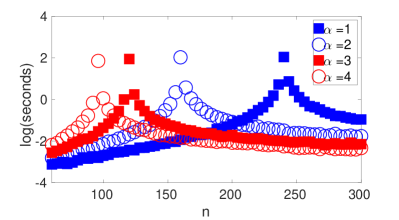
Figure 3: LRE and log-runtime of th-RegTME vs. number of samples $n,$ at $p=480$ and $\alpha=1,2,3,4$.

7.3 Regularized TME in the presence of outliers

We conclude the numerical section with an illustrative example of the ability of the regularized TME to detect outliers, and upon their removal and thresholding, to provide a robust and accurate estimate of a sparse shape matrix. For a related rigorous study on the ability of Maronna’s M-estimator to detect outliers, see Morales-Jimenez, Couillet and McKay (2015).

To this end, we consider the following $\epsilon$-contamination mixture model: $(1-\epsilon)n$ of the observed data, the inliers, follow an elliptical distribution with the same sparse shape matrix $\bm{S}_{p}$ as above. The remaining $\epsilon n$ of the samples, the outliers, follow an elliptical distribution with shape matrix $\bm{U}(p\bm{D}/tr(\bm{D}))\bm{U}^{\prime}$, where $\bm{U}$ is a unitary matrix, uniformly distributed with Haar measure, and $\bm{D}$ is a diagonal matrix. In our first experiment, the diagonal entries $d_{ii}$ are all i.i.d. uniformly distributed over $[1,5]$, so the outliers are rather diffuse. In our second experiment $d_{11}=p,d_{22}=p/2$ and all other $d_{ii}=1$, so the outliers are nearly on a 2-d randomly rotated subspace.

Given $n$ samples from this $\epsilon$-contamination model, and without knowledge of $\epsilon$, the task is to accurately estimate the shape matrix $\bm{S}_{p}$. Since both the inliers and outliers have potentially heavy tailed distributions, it might not be possible to detect the outliers by simple schemes, such as those based on the norm of a sample or the number of its neighbors in a given radius. However, recall that by our theoretical analysis, in the absence of outliers ($\epsilon=0$), the corresponding weights $w_{i}$ in the regularized TME are all approximately equal. For $\epsilon\ll 1$, with all samples normalized to have unit norm, we thus expect the inliers to still all have similar weights, and the outliers to have quite different weights, hopefully smaller though not necessarily so. With further details in Appendix A.10, our proposed procedure for robustness to outliers is to estimate the mean and standard deviation of the inliers’ weights. Then exclude all samples whose weights are outside, say, the mean plus or minus two standard deviations, recompute the regularized TME on the remaining samples and threshold it.

Fig. 4 illustrates the robustness of this procedure to outliers in two different settings. From left to right, for $\epsilon=0.2$ and $\epsilon=0.4$, it shows the weights of the $n$ normalized samples $\bm{x}_{i}/\|\bm{x}_{i}\|$, sorted so the first $\epsilon n$ of them are the outliers. The blue horizontal line is a robust estimate of the mean weight of the inliers, and the two red lines are this estimated mean plus and minus two standard deviations. The top row corresponds to the first outlier model with $d_{ii}\sim U[1,5]$. The second row corresponds to our second outlier model with $D=\operatorname{diag}(p,p/2,1,\ldots,1)$. Note that this outlier shape matrix has a spectral norm $O(p)$, which does not satisfy our requirement that $\|\bm{D}\|\leq s_{\max}$. As indeed observed empirically, the weights of the outliers do not so tightly concentrate around some value. Yet, our outlier exclusion procedure still succeeds to exclude most of these outliers. The error of the thresholded TME with outliers removed, compared to that of thresholding the original TME is shown in the right column of Fig. 4.

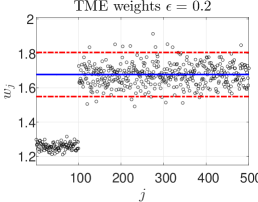
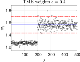
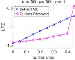
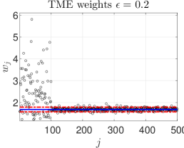
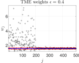
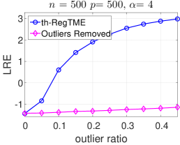
Figure 4: The TME weights for $\epsilon=0.2,0.4$ and the log relative error (LRE) of thresholding the regularized TME, before and after outlier removal, vs. $\epsilon$. Top row $D_{ii}\sim U[1,5]$. Bottom row $D=\operatorname{diag}(p,p/2,1,\ldots,1)$.

This simple example illustrates the potential ability of TME to screen outliers in high dimensional settings, at least for small contamination levels. A detailed study of this ability is an interesting topic for future research.

8 Summary and Discussion

In this paper we proposed simple estimators for the shape matrix of possibly heavy tailed elliptical distributions, assuming the shape matrix is approximately sparse. We further analyzed their error, showing that under the spectral norm they are minimax rate optimal in a high-dimensional setting with $p/n\to\gamma$.

There are several directions for future research. One direction is to extend our results to the case $p=n^{\beta}$, with $\beta>1$. Our current analysis assumed the regularization parameter $\alpha$ of TME is fixed, whereas if $p=n^{\beta}$ with $\beta>1$, just to ensure its existence would require $\alpha\to\infty$. Handling this case thus requires extending our analysis to allow $\alpha$ to grow with $n$ and $p$.

A question of practical interest is how to set the threshold parameter in a data-driven fashion. Bickel and Levina (2008, Section 3), proposed a cross validation procedure to set the threshold. Rigorously proving that this provides a good estimate in the case of (regularized) TME is an interesting topic for future work.

While our work focused on approximate sparsity of the shape matrix, robust inference under other common assumptions can also be studied. For example, one might assume that the first few leading eigenvectors of $\bm{\Sigma}$ are sparse, also known as sparse-PCA, or that $\bm{\Sigma}$ is the combination of a low rank and a sparse matrix. In particular, a robust sparse-PCA estimator may be constructed by applying a sparse-PCA procedure to Tyler’s M-estimator.

Finally, another direction for future work is to develop a computationally efficient algorithm for sparse covariance estimation in the presence of a small fraction of arbitrary outliers. This setting was considered in Chen, Gao and Ren (2018), but without a computationally tractable estimator. Our promising preliminary results in Section 7.3 suggest to study whether regularized TME offers such robustness, and under which outlier models.

Appendix A Supplementary Details

A.1 Complexity of Calculating the Regularized TME

Proof of Lemma 1.

We arbitrarily fix a solution $\bm{\hat{\Sigma}}(\alpha)$ of (4). Since $\bm{\hat{\Sigma}}(\alpha)$ is invariant to scaling of the data, we assume that $\|\bm{x}_{i}\|=1$, $1\leq i\leq n$. We first analyze the quantity $e_{1}=\|\bm{\hat{\Sigma}}(\alpha)-\bm{\hat{\Sigma}}_{1}(\alpha)\|$. To this end, let $\lambda_{\max}=\|\bm{\hat{\Sigma}}(\alpha)\|$. Taking the spectral norm in Eq. (4), together with the fact that $\frac{1}{\bm{x}^{T}\bm{\hat{\Sigma}}(\alpha)^{-1}\bm{x}}\leq\lambda_{\max}$ for any vector $\bm{x}$ with $\|\bm{x}\|=1$,

$$\lambda_{\max} \leq \tfrac{1}{1+\alpha}\left\|\tfrac{p}{n}\textstyle\sum_{i=1}^{n}\tfrac{\bm{x}_{i}\bm{x}_{i}^{T}}{\bm{x}_{i}^{T}\Sigma^{-1}\bm{x}_{i}}\right\|+\tfrac{\alpha}{1+\alpha}\leq\tfrac{1}{1+\alpha}\lambda_{\max}C(\bm{\tilde{}}{\bm{X}})+\tfrac{\alpha}{1+\alpha}.$$

Equivalently, for $1+\alpha>C(\bm{\tilde{}}{\bm{X}})$,

$$\lambda_{\max}\leq\frac{\alpha}{1+\alpha}\frac{1}{1-\frac{C(\bm{\tilde{}}{\bm{X}})}{1+\alpha}}.$$

Combining this inequality with the fact that by Eq. (4) $\bm{\hat{\Sigma}}(\alpha)-\frac{\alpha}{1+\alpha}\bm{I}\in S_{+}^{p}$,

$$e_{1}=\Big{\|}\bm{\hat{\Sigma}}(\alpha)-\frac{\alpha}{1+\alpha}\bm{I}\Big{\|}=\lambda_{\max}-\frac{\alpha}{1+\alpha}\leq\frac{C(\bm{\tilde{}}{\bm{X}})}{1+\alpha}\frac{\alpha}{1+\alpha}\frac{1}{1-\frac{C(\bm{\tilde{}}{\bm{X}})}{1+\alpha}}.$$ (25)

Next, we analyze the error $e_{k}$. We denote $\bm{E}_{k}=\bm{\hat{\Sigma}}(\alpha)-\bm{\hat{\Sigma}}_{k}(\alpha)$ and write

$$\bm{\hat{\Sigma}}_{k}(\alpha)=\bm{\hat{\Sigma}}(\alpha)-\bm{E}_{k}=\bm{\hat{\Sigma}}(\alpha)^{1/2}({\bm{I}}-\bm{\hat{\Sigma}}(\alpha)^{-1/2}\bm{E}_{k}\bm{\hat{\Sigma}}(\alpha)^{-1/2})\bm{\hat{\Sigma}}(\alpha)^{1/2}.$$

Since $\bm{\hat{\Sigma}}(\alpha)$ and $\bm{\hat{\Sigma}}_{k}(\alpha)$ are invertible, so is $\bm{I}-\bm{\hat{\Sigma}}(\alpha)^{-1/2}\bm{E}_{k}\bm{\hat{\Sigma}}(\alpha)^{-1/2}$. Let $\bm{B}_{k}={\bm{I}}-({\bm{I}}-\bm{\hat{\Sigma}}(\alpha)^{-1/2}\bm{E}_{k}\bm{\hat{\Sigma}}(\alpha)^{-1/2})^{-1}$ and $\bm{R}_{k}=\bm{\hat{\Sigma}}(\alpha)^{-1/2}\bm{B}_{k}\bm{\hat{\Sigma}}(\alpha)^{-1/2}$. Then,

$$\bm{\hat{\Sigma}}_{k}(\alpha)^{-1}=\bm{\hat{\Sigma}}(\alpha)^{-1/2}(\bm{I}-\bm{B}_{k})\bm{\hat{\Sigma}}(\alpha)^{-1/2}=\bm{\hat{\Sigma}}(\alpha)^{-1}-\bm{R}_{k}.$$

Subtracting Eq. (5) from Eq. (4) gives

$$\bm{E}_{k+1} = \frac{1}{1+\alpha}\frac{p}{n}\sum_{i}\bm{x}_{i}\bm{x}_{i}^{T}\left(\frac{1}{\bm{x}_{i}^{T}\bm{\hat{\Sigma}}(\alpha)^{-1}\bm{x}_{i}}-\frac{1}{\bm{x}_{i}^{T}\bm{\hat{\Sigma}}(\alpha)^{-1}\bm{x}_{i}-\bm{x}_{i}^{T}\bm{R}_{k}\bm{x}_{i}}\right)$$

$$= \frac{1}{1+\alpha}\frac{p}{n}\sum_{i}\frac{\bm{x}_{i}\bm{x}_{i}^{T}}{\bm{x}_{i}^{T}\bm{\hat{\Sigma}}(\alpha)^{-1}\bm{x}_{i}}\left(1-\frac{1}{1-\delta_{ki}}\right),$$

where $\delta_{ki}=\bm{x}_{i}^{T}\bm{R}_{k}\bm{x}_{i}/\bm{x}_{i}^{T}\bm{\hat{\Sigma}}(\alpha)^{-1}\bm{x}_{i}$.

Let $D_{k}=\max_{1\leq i\leq n}|\delta_{ki}/(1-\delta_{ki})|$. Since all terms $\bm{x}_{i}\bm{x}_{i}^{T}/\bm{x}_{i}^{T}\bm{\hat{\Sigma}}(\alpha)^{-1}\bm{x}_{i}$ are positive semidefinite, the above equation implies that

$$\|\bm{E}_{k+1}\|\leq D_{k}\left\|\tfrac{1}{1+\alpha}\tfrac{p}{n}\textstyle\sum_{i}\tfrac{\bm{x}_{i}\bm{x}_{i}^{T}}{\bm{x}_{i}^{T}\bm{\hat{\Sigma}}(\alpha)^{-1}\bm{x}_{i}}\right\|=D_{k}\left\|\bm{\hat{\Sigma}}(\alpha)-\tfrac{\alpha}{1+\alpha}\bm{I}\right\|=D_{k}e_{1}.$$ (26)

Eq. (25) gives a bound on $e_{1}$. We now bound $D_{k}$. Since $\bm{\hat{\Sigma}}(\alpha)\geq\frac{\alpha}{1+\alpha}\bm{I}$,

$$\|\bm{\hat{\Sigma}}(\alpha)^{-1/2}\bm{E}_{k}\bm{\hat{\Sigma}}(\alpha)^{-1/2}\|\leq\|\bm{\hat{\Sigma}}(\alpha)^{-1}\|e_{k}\leq\frac{1+\alpha}{\alpha}e_{k}.$$

Assume this quantity is strictly smaller than one, then

$$\|\bm{B}_{k}\|=\|{\bm{I}}-({\bm{I}}-\bm{\hat{\Sigma}}(\alpha)^{-1/2}\bm{E}_{k}\bm{\hat{\Sigma}}(\alpha)^{-1/2})^{-1}\|\leq\frac{1+\alpha}{\alpha}\frac{e_{k}}{1-\frac{1+\alpha}{\alpha}e_{k}}.$$ (27)

Finally, given the relation between $\bm{R}_{k}$ and $\bm{B}_{k}$,

$$|\delta_{ki}|=\frac{|\bm{x}_{i}^{T}\bm{R}_{k}\bm{x}_{i}|}{\bm{x}_{i}^{T}\bm{\hat{\Sigma}}(\alpha)^{-1}\bm{x}_{i}}=\frac{|(\bm{\hat{\Sigma}}(\alpha)^{-1/2}\bm{x}_{i})^{T}\bm{B}_{k}(\bm{\hat{\Sigma}}(\alpha)^{-1/2}\bm{x}_{i})|}{\|\bm{\hat{\Sigma}}(\alpha)^{-1/2}\bm{x}_{i}\|^{2}}\leq\|\bm{B}_{k}\|.$$

Thus, assuming $\|\bm{B}_{k}\|<1$,

$$D_{k}=\max_{i}\frac{|\delta_{ki}|}{1-\delta_{ki}}\leq\frac{\|\bm{B}_{k}\|}{1-\|\bm{B}_{k}\|}=\frac{1+\alpha}{\alpha}e_{k}\cdot\frac{1}{1-2\frac{1+\alpha}{\alpha}e_{k}}.$$ (28)

Inserting (28) and (25) into (26) yields that

$$\frac{e_{k+1}}{e_{k}}\leq\frac{C(\bm{\tilde{}}{\bm{X}})}{1+\alpha}\frac{1}{1-\frac{C(\bm{\tilde{}}{\bm{X}})}{1+\alpha}}\frac{1}{1-2\frac{1+\alpha}{\alpha}e_{k}}.$$ (29)

For the proof to hold, we required that $\frac{1+\alpha}{\alpha}e_{k}<1$ and $\|\bm{B}_{k}\|<1$. If $\frac{1+\alpha}{\alpha}e_{k}<0.5$, then the RHS of Eq. (27) is less than one and both assumptions hold. For $0<R<1$ and $1+\alpha>(3+R^{-1})C(\bm{\tilde{}}{\bm{X}})$, Eq. (25) implies that $\frac{1+\alpha}{\alpha}e_{1}<\frac{1}{2+R^{-1}}$ and combining this with Eq. (29) results in the estimate $e_{2}/e_{1}<R$. Since $R<1$, easy induction implies that for $k>1$, $\frac{1+\alpha}{\alpha}e_{k}<\frac{1}{2+R^{-1}}<0.5$, as required, and so Eq. (6) holds. Since this convergence holds with any solution of (4), this solution thus has to be unique. ∎

Proof of Lemma 2.

Since the regularized TME is invariant to scaling, we may assume that all $u_{i}\sim\chi^{2}_{p}$, and express $\bm{x}_{i}=\bm{S}_{p}^{\frac{1}{2}}\bm{\xi}_{i}$, where $\bm{\xi}_{i}\sim N(\bm{0},\bm{I}).$ Let $\bm{U}\bm{D}\bm{U}^{T}$ be the eigendecomposition of $\bm{S}_{p}$. Redefining $\bm{\xi}=\bm{U}\bm{\xi}$, then $\|\bm{x}_{i}\|^{2}=\bm{\xi}_{i}^{T}\bm{D}\bm{\xi}_{i}$ and

$$C(\bm{\tilde{}}{\bm{X}})=\left\|\bm{S}_{p}^{\frac{1}{2}}\left(\frac{1}{n}\sum_{i=1}^{n}\frac{\bm{\xi}_{i}\bm{\xi}_{i}^{T}}{\frac{1}{p}\bm{\xi}_{i}^{T}\bm{D}\bm{\xi}_{i}}\right)\bm{S}_{p}^{\frac{1}{2}}\right\|.$$

Combining Lemma 5 with a union bound yields

$$\operatorname{Pr}\left(\max_{i}\left|\frac{1}{p}\bm{\xi}_{i}^{T}\bm{D}\bm{\xi}_{i}-\frac{1}{p}\operatorname{tr}(\bm{D})\right|>\epsilon\right)<2n\exp\left(-c_{1}\min\left\{\frac{c_{2}^{2}p^{2}\epsilon^{2}}{\|\bm{D}\|_{F}^{2}},\frac{c_{2}p\epsilon}{\|\bm{D}\|}\right\}\right).$$

Since $\|\bm{D}\|=\|\bm{S}_{p}\|$ and $\|\bm{D}\|_{F}^{2}\leq p\|\bm{S}_{p}\|^{2}$, for any fixed $\epsilon$ the above probability is exponentially small in $p$. Taking say $\epsilon=1/2$ and recalling that $\operatorname{tr}(\bm{D})=p$, gives that with high probability,

$$C(\bm{\tilde{}}{\bm{X}})\leq 2\|\bm{S}_{p}\|\cdot\Big{\|}\frac{1}{n}\sum_{i=1}^{n}\bm{\xi}_{i}\bm{\xi}_{i}^{T}\Big{\|}.$$

Eq. (7) follows since by Lemma 4, w.h.p. $\|\frac{1}{n}\sum_{i=1}^{n}\bm{\xi}_{i}\bm{\xi}_{i}^{T}\|\leq(1+2\sqrt{p/n})^{2}$. ∎

A.2 Proof of Lemma 6

Most of the proof follows Bickel and Levina (2008, p. 2583). By the triangle inequality,

$$\|\tau_{t}(\bm{A})-\bm{B}\|\leq\|\tau_{t}(\bm{B})-\bm{B}\|+\|\ \tau_{t}(\bm{A})-\tau_{t}(\bm{B})\|=q_{1}+q_{2}.$$

As in their Eq. (13), $q_{1}\leq t^{1-q}s_{p}$. For the second term $q_{2}$,

$$q_{2} \leq \max_{i}\sum_{j=1}^{p}|a_{ij}|\bm{1}(|a_{ij}|\geq t,|b_{ij}|<t)+\max_{i}\sum_{j=1}^{p}|b_{ij}|\bm{1}(|a_{ij}|<t,|b_{ij}|\geq t)$$

$$+\max_{i}\sum_{j=1}^{p}|a_{ij}-b_{ij}|\bm{1}(|a_{ij}|\geq t,|b_{ij}|\geq t)=q_{3}+q_{4}+q_{5}.$$

Similarly, $q_{4}\leq C_{1}\sqrt{\frac{\log p}{n}}t^{-q}s_{p}+t^{1-q}s_{p}$ and $q_{5}\leq C_{1}\sqrt{\frac{\log p}{n}}t^{-q}s_{p}$. For $q_{3}$,

$$q_{3}\leq\max_{i}\sum_{j=1}^{p}|a_{ij}-b_{ij}|\bm{1}(|a_{ij}|\geq t,|b_{ij}|<t)+\max_{i}\sum_{j=1}^{p}|b_{ij}|\bm{1}(|a_{ij}|\geq t,|b_{ij}|<t).$$

The second sum is bounded as above by $t^{1-q}s_{p}$. For the first sum, we slightly differ from Bickel and Levina (2008). Since $|a_{ij}-b_{ij}|\leq C_{1}\sqrt{\frac{\log p}{n}}$ and $t=K\sqrt{\frac{\log p}{n}}$ with $K>C_{1}$ then all terms satisfy $|b_{ij}|>t(1-C_{1}/K).$ Hence,

$$q_{3} \leq C_{1}\sqrt{\tfrac{\log p}{n}}\max_{i}\sum_{j=1}^{p}\bm{1}\left(|b_{ij}|>t\left(1-\tfrac{C_{1}}{K}\right)\right)+t^{1-q}s_{p}$$

$$\leq C_{1}\sqrt{\tfrac{\log p}{n}}t^{-q}(1-\tfrac{C_{1}}{K})^{-q}s_{p}+t^{1-q}s_{p}.$$

Collecting the above inequalities concludes the proof, since

$$\|\tau_{t}(\bm{A})-\bm{B}\|\leq\left(3K^{1-q}+C_{1}K^{-q}(2+(1-C_{1}/K)^{-q})\right)s_{p}\left(\frac{\log p}{n}\right)^{\frac{1-q}{2}}.$$

A.3 Proof of Lemma 7

Let $\bm{x}_{i}=\bm{S}_{p}^{1/2}\bm{y}_{i}$ where $\bm{y}_{i}$ are i.i.d. $N(0,\bm{I})$. Let $\hat{\bm{\Sigma}}_{x}$ and $\hat{\bm{\Sigma}}_{y}$ be their TME’s, respectively. It follows directly from Eq. (12) that the weights $\{w_{i}^{x}\}_{i=1}^{n}$ and $\{w_{i}^{y}\}_{i=1}^{n}$ are identical. The latter are tightly concentrated around $1/n$ by Zhang, Cheng and Singer (2016, Lemma 2.2).

A.4 Proof of Lemma 8

Since $\bm{x}_{i}\sim N({\bm{0}},\bm{S}_{p}),$ by Lemma 7 the TME weights $\bm{w}=(w_{1},\ldots,w_{n})^{T}$ of Eq. (12) are all concentrated around $1/n$. The following lemma shows that $T_{w}=\operatorname{tr}(\sum_{i}w_{i}\bm{x}_{i}\bm{x}_{i}^{T})$ is close to $\operatorname{tr}(\bm{S}_{p})=p$.

Lemma 14.

Assume the setting of Lemma 8. There exist constants $C,c$ and $c^{\prime}<1$ depending on $\gamma$ such that $\forall\epsilon\in(0,c^{\prime})$ and $n$ sufficiently large,

$$\Pr\left(\left|\tfrac{p}{T_{w}}-1\right|>\epsilon\right)\leq Cne^{-cn\epsilon^{2}}.$$ (30)

We prove Lemma 8 assuming Lemma 14 holds, and then prove the latter.

Proof of Lemma 8.

By definition,

$$\|\bm{\hat{\Sigma}}-\bm{\hat{S}}\|_{\max}=\Big{\|}\sum_{i=1}^{n}\left(\tfrac{pw_{i}}{T_{w}}-\tfrac{1}{n}\right)\bm{x_{i}x_{i}}^{T}\Big{\|}_{\max}\leq\left\|\tfrac{np{\bm{w}}}{T_{w}}-{\bm{1}}\right\|_{\infty}\cdot\Big{\|}\tfrac{1}{n}\sum_{i=1}^{n}\bm{x_{i}x_{i}}^{T}\Big{\|}_{\max}.$$ (31)

Since $\bm{x}_{i}\sim N(0,\bm{S}_{p})$ with $\bm{S}_{p}\in\mathcal{U}(q,s_{p},M)$, then w.h.p., $\|\frac{1}{n}\sum\bm{x}_{i}\bm{x}_{i}^{T}\|_{\max}\leq 2M$. As for the first term on the RHS of Eq. (31), by the triangle inequality,

$$\left\|\tfrac{np{\bm{w}}}{T_{w}}-{\bm{1}}\right\|_{\infty}=\left\|\tfrac{np{\bm{w}}}{T_{w}}-n\bm{w}+n\bm{w}-{\bm{1}}\right\|_{\infty}\leq\|n\bm{w}\|_{\infty}\left|\tfrac{p}{T_{w}}-1\right|+\|n\bm{w}-{\bm{1}}\|_{\infty}.$$

Hence,

$$\Pr\left(\left\|\tfrac{np{\bm{w}}}{T_{w}}-{\bm{1}}\right\|_{\infty}>\epsilon\right)\leq\Pr(\|n\bm{w}\|_{\infty}|\tfrac{p}{T_{w}}-1|>\epsilon/2)+\Pr(\|n\bm{w}-{\bm{1}}\|_{\infty}>\epsilon/2).$$

Lemma 7 provides an exponential bound on the second term. For the first term, applying Eq. (10) with $\lambda=2$ gives

$$\Pr(\|n\bm{w}\|_{\infty}|\tfrac{p}{T_{w}}-1|>\epsilon/2) \leq \ \Pr(\|n\bm{w}\|_{\infty}>2)+\Pr(|\tfrac{p}{T_{w}}-1|>\epsilon/4)$$

$$\leq \Pr(\|n\bm{w}-{\bm{1}}\|_{\infty}>1)+\Pr(|\tfrac{p}{T_{w}}-1|>\epsilon/4).$$

By Lemmas 7 and 14, these two probabilities are exponentially small. ∎

Proof of Lemma 14.

As $|\tfrac{p}{T_{w}}-1|=\tfrac{p}{T_{w}}|1-\tfrac{T_{w}}{p}|$, by Eq. (10) with $\lambda=2$

$$\Pr\left(\tfrac{p}{T_{w}}|1-\tfrac{T_{w}}{p}|>\epsilon\right) \leq \Pr\left(\tfrac{p}{T_{w}}>2\right)+\Pr\left(|1-\tfrac{T_{w}}{p}|>\epsilon/2\right)$$

$$\leq \Pr\left(|\tfrac{T_{w}}{p}-1|>1/2\right)+\Pr\left(|1-\tfrac{T_{w}}{p}|>\epsilon/2\right)$$

$$\leq 2\Pr\left(|1-\tfrac{T_{w}}{p}|>\epsilon/2\right).$$

Next, we relate $|1-\tfrac{T_{w}}{p}|$ to $|1-\tfrac{T}{p}|$, where $T=\operatorname{tr}(\frac{1}{n}\sum_{i=1}^{n}\bm{x}_{i}\bm{x}_{i}^{T})$. Note that

$$|1-\tfrac{T_{w}}{p}| \leq |1-\tfrac{T}{p}|+|\tfrac{T}{p}-\tfrac{T_{w}}{p}|=|1-\tfrac{T}{p}|+\tfrac{1}{p}\left|\sum_{i=1}^{n}(\tfrac{1}{n}-w_{i})\bm{x}_{i}^{T}\bm{x}_{i}\right|$$

$$\leq |1-\tfrac{T}{p}|+\|n\bm{w}-\bm{1}\|_{\infty}\cdot|\tfrac{T}{p}|.$$

Therefore

$$\Pr\left(|1-\tfrac{T_{w}}{p}|>\tfrac{\epsilon}{2}\right)\leq\Pr\left(|1-\tfrac{T}{p}|>\tfrac{\epsilon}{4}\right)+\Pr\left(\|n\bm{w}-\bm{1}\|_{\infty}\cdot|\tfrac{T}{p}|>\tfrac{\epsilon}{4}\right)=q_{1}+q_{2}.$$

Applying Eq. (10) with $\lambda=2$ to the second term gives

$$q_{2} \leq \Pr\left(\|n\bm{w}-\bm{1}\|_{\infty}>\epsilon/8\right)+\Pr\left(\tfrac{T}{p}>2\right)$$

$$\leq \Pr\left(\|n\bm{w}-\bm{1}\|_{\infty}>\epsilon/8\right)+\Pr\left(|1-\tfrac{T}{p}|>1\right).$$

By Lemma 7, the first probability above has the desired exponential decay. To conclude the proof, we thus need to provide an exponential bound on $q_{1}$.

Let $\lambda_{1}\geq\lambda_{2}\geq\ldots\geq\lambda_{p}$ be the eigenvalues of $\bm{S}_{p}$. Since $\bm{x}_{i}\sim N({\bm{0}},\bm{S}_{p})$,

$$T=\operatorname{tr}\left(\frac{1}{n}\sum_{i=1}^{n}\bm{x}_{i}\bm{x}_{i}^{T}\right) = \sum_{j=1}^{p}\lambda_{j}\chi_{j}^{2}(n)/n,$$

where the $\chi^{2}_{j}(n)$ are i.i.d. chi-square random variables with $n$ degrees of freedom for $j=1,2,\dots,p$. Given that $\operatorname{tr}(\bm{S}_{p})=\sum_{j=1}^{n}\lambda_{j}=p$,

$$\left|1-\frac{T}{p}\right|=\frac{1}{p}\left|\sum_{j=1}^{p}\lambda_{j}\left(1-\frac{\chi_{j}^{2}(n)}{n}\right)\right|\leq\max_{j}\left|\frac{\chi_{j}^{2}(n)}{n}-1\right|.$$

Since $\chi^{2}$ random variables are sub-exponential, for a suitable constant $c>0,$

$${\rm{Pr}}\left(\bigg{|}\frac{\chi^{2}(n)}{n}-1\bigg{|}>\epsilon\right)<\exp\left(-cn\epsilon^{2}\right).$$ (32)

Therefore by a union bound, the term $q_{1}$ is also exponentially small. ∎

A.5 Proof of Proposition 1

To prove the existence of a unique $r^{*}=r^{*}(p,n,\alpha,\bm{S}_{p})$ which satisfies Eq. (14), we first show that $\mathbb{E}[Q(r)]$ is strictly monotone increasing in $r$ and then use the intermediate value theorem.

To simplify notation, let $\bm{T}=\frac{1}{n}\sum_{j=1}^{n-1}\bm{\xi}_{j}\bm{\xi}_{j}^{T}$ and $\beta=\beta(r)=\frac{n\alpha}{pr}$. Then

$$\mathbb{E}[Q(r)]=\mathbb{E}_{\bm{\xi}_{i}}[\mathbb{E}_{\bm{y}}[Q(r)]]=\mathbb{E}\left[\frac{1}{p}\operatorname{tr}\left(\left(\bm{T}+\beta\bm{S}_{p}^{-1}\right)^{-1}\right)\right],$$ (33)

where the expectation is now only over the random variables $\bm{\xi}_{i}$.

First, we show that for any fixed $\bm{S}_{p}\in\mathcal{S}_{p}^{++}$, $\mathbb{E}[Q(r)]$ is strictly monotone increasing in $r$. Indeed, taking the derivative with respect to $r$ and using the identity $\operatorname{tr}(\bm{A}\bm{B})=\operatorname{tr}(\bm{B}\bm{A})$ gives that

$$\frac{d}{dr}\mathbb{E}[Q(r)]=\frac{n\alpha}{pr^{2}}\,\mathbb{E}\left[\frac{1}{p}\operatorname{tr}((\bm{T}+\beta\bm{S}_{p}^{-1})^{-2}\bm{S}_{p}^{-1})\right].$$

Applying Bhatia (2013)[Prob. III.6.14] and Jensen’s inequality,

$$\frac{d}{dr}\mathbb{E}[Q(r)] \geq \frac{n\alpha}{pr^{2}}\lambda_{\min}(\bm{S}_{p}^{-1})\mathbb{E}[\frac{1}{p}\operatorname{tr}((\bm{T}+\beta\bm{S}_{p}^{-1})^{-2})]$$

$$\geq \frac{n\alpha}{pr^{2}}\frac{1}{s_{\max}}\mathbb{E}[1/\lambda_{1}(\bm{T}+\beta\bm{S}_{p}^{-1})^{2}]$$

$$\geq \frac{n\alpha}{pr^{2}}\frac{1}{s_{\max}}\frac{1}{\mathbb{E}[\lambda_{1}(\bm{T}+\beta\bm{S}_{p}^{-1})]^{2}}.$$

Clearly, $\lambda_{1}(\bm{T}+\beta\bm{S}_{p}^{-1})\leq\lambda_{1}(\bm{T})+\beta/{\lambda_{\min}(\bm{S}_{p})}$. Furthermore, upon averaging over the random variables $\bm{\xi}_{i}$, by Lemma 4, $\mathbb{E}[\lambda_{1}(\bm{T})]\leq(1+\sqrt{p/n})^{2}$. Therefore, for any fixed $\bm{S}_{p}$, the derivative of $\mathbb{E}[Q(r)]$ is strictly positive for any $r>0$. Hence if there exists a solution to Eq. (14), then it must be unique.

Next, we show that this solution must satisfy $r\geq r_{\min}$. By definition,

$$\mathbb{E}[Q(r)] = \frac{1}{p}\sum_{j=1}^{n}\frac{1}{\lambda_{j}(\bm{T}+\beta\bm{S}_{p}^{-1})}$$ (34)

$$\leq \frac{1}{p}\sum_{j=1}^{n}\frac{1}{\lambda_{j}(\beta\bm{S}_{p}^{-1})}=\frac{1}{\beta}\frac{1}{p}\sum_{j=1}^{p}\lambda_{j}(\bm{S}_{p})=\frac{n\alpha}{pr}.$$

Combining (34) with (14) implies that

$$r^{*}(p,n,\alpha,\bm{S}_{p})\geq\frac{n}{p}\frac{\alpha}{1+\alpha-p/n}=r_{\min}.$$

Finally, we bound $r$ from above. To this end, note that

$$\mathbb{E}[Q(r)] = \frac{1}{p}\mathbb{E}\left[\sum_{j}\frac{1}{\lambda_{j}(\bm{T}+\beta\bm{S}_{p}^{-1})}\right]\geq\frac{1}{p}\mathbb{E}\left[\sum_{j}\frac{1}{\beta/\lambda_{j}(\bm{S}_{p})+\|\bm{T}\|}\right]$$

$$\geq \mathbb{E}\left[\frac{1}{\beta+s_{\max}\|\bm{T}\|}\right]\geq\frac{1}{\beta+s_{\max}\mathbb{E}[\|\bm{T}\|]}$$

where the last inequality is Jensen’s inequality. By Lemma 4, $\mathbb{E}[\|\bm{T}\|]\leq(1+\sqrt{p/n})^{2}$. Hence, for $\alpha>p/n-1+s_{\max}(1+\sqrt{p/n})^{2}$, the solution to Eq. (14) satisfies

$$r^{*}\leq r_{\max}=\frac{n}{p}\frac{\alpha}{1+\alpha-p/n-s_{\max}(1+\sqrt{\gamma})^{2}}.$$

A.6 Proof of Lemma 9

Let $\hat{\bm{S}}=\frac{1}{n}\sum_{k=1}^{n}\bm{x}_{k}\bm{x}_{k}^{T}$ and $\hat{\bm{T}}=\frac{1}{n}\sum_{k=1}^{n}\bm{\xi}_{k}\bm{\xi}_{k}^{T}$, where $\bm{x}_{i}=\bm{S}_{p}^{\frac{1}{2}}\bm{\xi}_{i}$ and $\bm{\xi}_{i}\overset{iid}{\sim}N(\bm{0},\bm{I})$. Then, Eq. (18) may be written as

$$\frac{1}{r}g(\bm{u})_{i} = 1-\frac{1/(1+\alpha)}{\frac{1}{p}\bm{x}_{i}^{T}\left(\hat{\bm{S}}+\beta\bm{I}\right)^{-1}\bm{x}_{i}}=1-\frac{1/(1+\alpha)}{\frac{1}{p}\bm{\xi}_{i}^{T}\left(\bm{S}_{p}^{-\frac{1}{2}}\hat{\bm{S}}\bm{S}_{p}^{-\frac{1}{2}}+\beta\bm{S}_{p}^{-1}\right)^{-1}\bm{\xi}_{i}}$$ (35)

$$= 1-\frac{1}{1+\alpha}\frac{1}{\frac{1}{p}\bm{\xi}_{i}^{T}\bm{E}\bm{\xi}_{i}},$$

where $\bm{E}=\left(\hat{\bm{T}}\bm{+}\beta\bm{S}_{p}^{-1}\right)^{-1}$ and $\beta=\alpha\frac{n}{p}\frac{1}{r}$. The quadratic form $\frac{1}{p}\bm{\xi}_{i}^{T}\bm{E}\bm{\xi}_{i}$ is difficult to analyze directly because $\bm{E}$ depends on ${\bm{\xi}}_{i}$. To disentangle this dependency, let $\hat{\bm{T}}_{-i}=\frac{1}{n}\sum_{k\neq i}\bm{\xi}_{k}\bm{\xi}_{k}^{T}$, and $\bm{E}_{-i}=(\hat{\bm{T}}_{-i}+\beta\bm{S}_{p}^{-1})^{-1}$. As $\bm{E}^{-1}$ and $\bm{E}_{-i}^{-1}$ differ by a rank-one matrix $\frac{1}{n}\bm{\xi}_{i}\bm{\xi}_{i}^{T}$, by the Sherman-Morrison formula,

$$\bm{E}=\bm{E}_{-i}-\frac{1}{n}\frac{\bm{E}_{-i}\bm{\xi}_{i}\bm{\xi}_{i}^{T}\bm{E}_{-i}}{1+\frac{1}{n}\bm{\xi}_{i}^{T}\bm{E}_{-i}\bm{\xi}_{i}}.$$

Therefore, denoting by $Q_{i}$ the quadratic form

$$Q_{i}(r)\equiv Q_{i}=\frac{1}{p}\bm{\xi}_{i}^{T}\bm{E}_{-i}\bm{\xi}_{i},$$ (36)

it follows that

$${\frac{1}{p}\bm{\xi}_{i}^{T}\bm{E}\bm{\xi}_{i}}=Q_{i}-\frac{\frac{p}{n}Q_{i}^{2}}{1+\frac{p}{n}Q_{i}}=\frac{Q_{i}}{1+\frac{p}{n}Q_{i}}.$$ (37)

Plugging this expression into Eq. (35) gives

$$\frac{1}{r}g(\bm{u})_{i}=\frac{Q_{i}(1+\alpha-\frac{p}{n})-1}{(1+\alpha)Q_{i}}.$$ (38)

Next, to establish a concentration bound for $g(\bm{u})_{i}/r$, we study the concentration of $Q_{i}$. Since $\bm{\xi}_{i}\sim N({\bm{0}},{\bm{I}})$ and is independent of $\bm{E}_{-i}$,

$$\mathbb{E}Q_{i}=\mathbb{E}\operatorname{tr}(\bm{E}_{-i})/p.$$

We first show that $Q_{i}$ concentrates tightly around ${\operatorname{tr}}(\bm{E}_{-i})/p$ in view of concentration of quadratic forms. We then show that ${\operatorname{tr}}(\bm{E}_{-i})$ concentrates tightly around its mean using results about the concentration of certain functions of the eigenvalues of random matrices.

Applying Lemma 5 with $\bm{\xi}=\bm{\xi}_{i}$ and viewing the matrix $\bm{E}_{-i}$ as fixed,

$$\Pr\left(\left|Q_{i}-\frac{1}{p}\operatorname{tr}\left(\bm{E}_{-i}\right)\right|>\epsilon\right)\leq 2\exp\left(-c_{1}\min\left\{\frac{c_{2}^{2}p^{2}\epsilon^{2}}{\left\|\bm{E}_{-i}\right\|_{F}^{2}},\frac{c_{2}p\epsilon}{\left\|\bm{E}_{-i}\right\|}\right\}\right),$$

where the above probability is only w.r.t. $\bm{\xi}_{i}$. Next, given that $\bm{E}_{-i}=(\bm{T}_{-i}+\beta\bm{S}_{p}^{-1})^{-1}$, then $\|\bm{E}_{-i}\|\leq\frac{s_{\max}}{\beta}$ and $\|\bm{E}_{-i}\|_{F}^{2}\leq ps_{\max}^{2}/\beta^{2}$. Thus,

$$\Pr\left(\left|Q_{i}-\frac{1}{p}{\operatorname{tr}}\left(\bm{E}_{-i}\right)\right|>\epsilon\right)\leq C\exp\left(-cp\epsilon^{2}\right),$$ (39)

where now the probability is over all of the $\bm{\xi}_{k}$’s.

It remains to obtain a concentration inequality for ${\operatorname{tr}}\left(\bm{E}_{-i}\right)/p$. To this end, consider the following $p\times(n-1+p)$ matrix,

$${\bm{Y}}=\left(\begin{array}[]{cccccc|ccc}{\bm{\xi}}_{1}&\cdots&{\bm{\xi}}_{i-1}&{\bm{\xi}}_{i+1}&\cdots&{\bm{\xi}}_{n}&\sqrt{n\beta}\bm{S}_{p}^{-1/2}\end{array}\right).$$

By definition, all entries of ${\bm{Y}}$ are independent, the first $p\times(n-1)$ are standard Gaussian random variables and the rest deterministic. Then, by Guionnet and Zeitouni (2000)[Corollary 1.8b], for any function $h:\mathbb{R}\to\mathbb{R}$ such that $h(x^{2})$ is Lipschitz with constant $L$, for any $\delta>0$

$$\Pr\left(\tfrac{1}{K}\left|\operatorname{tr}h(\tfrac{{\bm{Y}}{\bm{Y}^{T}}}{K})-\mathbb{E}\operatorname{tr}(h(\tfrac{{\bm{Y}}{\bm{Y}^{T}}}{K}))\right|>\delta\right)\leq 2\exp\left(-\tfrac{\delta^{2}K^{2}}{2L^{2}}\right)$$ (40)

where $K=2p+n-1$ and for a symmetric matrix $\bm{A}$ with eigenvalues $\lambda_{j}$, $\operatorname{tr}h(\bm{A})=\sum_{j}h(\lambda_{j})$.

Since ${\bm{Y}}{\bm{Y}}^{T}=n(\hat{\bm{T}}_{-i}+\beta\bm{S}_{p}^{-1})=n\bm{E}_{-i}^{-1}$, consider the function

$$h(x)=\frac{n}{p}\cdot\frac{1}{x}$$

for which $\frac{1}{2p+n-1}\operatorname{tr}h({\bm{Y}}{\bm{Y}}^{T}/(2p+n-1))=\operatorname{tr}(\bm{E}_{-i})/p$. Next, note that for sufficiently large $n$ and sufficiently small $\epsilon$

$$\lambda_{\min}\left(\frac{\bm{Y}\bm{Y}^{T}}{2p+n-1}\right)=\frac{n}{2p+n-1}\lambda_{\min}(\hat{\bm{T}}_{-i}+\beta\bm{S}_{p}^{-1})\geq\frac{1}{2\gamma+1+\epsilon}\frac{\beta}{s_{\max}}=x_{0}.$$

We thus apply the function $h$ only in the interval $x\geq x_{0}$. The Lipschitz constant of $h(x^{2})$ for $n$ sufficiently large is bounded by

$$L\leq\left|\frac{d}{dx}h(x^{2})\bigg{|}_{x=x_{0}}\right|\leq 16\frac{(\gamma+0.5+\epsilon)^{3}}{\gamma-\epsilon}\left(\frac{s_{\max}}{\beta}\right)^{3}\leq 16\frac{(\gamma+1)^{3}}{\gamma}\left(\frac{s_{\max}}{\beta}\right)^{3}.$$

Hence, applying (40), there exists a positive constant $c$ that depends on $\gamma,\alpha,r$ and $s_{\max}$ such that

$$\Pr\left(\frac{1}{p}\left|\operatorname{tr}(\bm{E}_{-i})-\mathbb{E}\operatorname{tr}(\bm{E}_{-i})\right|>\delta\right)\leq 2\exp\left(-cp^{2}\delta^{2}\right).$$ (41)

Next, by the triangle inequality

$$\Pr(|Q_{i}-\tfrac{\mathbb{E}\operatorname{tr}(\bm{E}_{-i})}{p}|>\epsilon)\leq\Pr\left(|Q_{i}-\tfrac{\operatorname{tr}(\bm{E}_{-i})}{p}|>\tfrac{\epsilon}{2}\right)+\Pr\left(|\tfrac{\operatorname{tr}(\bm{E}_{-i})}{p}-\tfrac{\mathbb{E}\operatorname{tr}(\bm{E}_{-i})}{p}|>\tfrac{\epsilon}{2}\right)$$

Combining the above equation with Eqs. (39) and (41), implies that at the value of $r$ specified in Proposition 1, for which $\mathbb{E}\left[\operatorname{tr}(\bm{E}_{-i})/p\right]=\frac{1}{1+\alpha-\frac{p}{n}}$,

$${\rm{Pr}}\left(\left|Q_{i}-\frac{1}{1+\alpha-\frac{p}{n}}\right|>\epsilon\right)<Ce^{-cp\epsilon^{2}}.$$ (42)

We are finally ready to establish a concentration result for $\frac{1}{r}g(\bm{u})$. Combining Eq. (38) and a union bound over all $p$ coordinates of $g$,

$$\Pr\left(\left\|\tfrac{1}{r}g(\bm{u})\right\|_{\infty}>\epsilon\right)\leq p\Pr\left(\left|\tfrac{1}{r}g(\bm{u})_{i}\right|>\epsilon\right)\leq p\Pr\left(\left|\tfrac{Q_{i}(1+\alpha-p/n)-1}{(1+\alpha)Q_{i}}\right|>\epsilon\right).$$

Applying Eq. (10) with $\lambda=1$ to the equation above gives

$$\Pr\left(\left\|\tfrac{1}{r}g(\bm{u})\right\|_{\infty}>\epsilon\right)<p\Pr\left(\left|Q_{i}(1+\alpha-\tfrac{p}{n})-1)\right|>\epsilon\right)+p\Pr\left((1+\alpha)Q_{i}<1\right).$$

By Eq. (42), the first term on the RHS is exponentially small in $p$. As for the second term, since $(1+\alpha)^{-1}<(1+\alpha-p/n)^{-1}$, then again by Eq. (42), $\Pr(Q_{i}<1/(1+\alpha))$ is also exponentially small in $p$. The lemma thus follows from the boundedness of $r$ from above, as established in Proposition 1.

A.7 Proof of Lemma 10

For any $\bm{v}\in\mathbb{R}^{n}$, denote $\hat{\bm{S}}(\bm{v})=\frac{1}{n}\sum_{k}v_{k}\bm{x}_{k}\bm{x}_{k}^{T}$ and

$$\bm{F}(\bm{v})=\left(\frac{1}{r}\hat{\bm{S}}(\bm{v})+\beta\bm{I}\right)^{-1}.$$ (43)

We prove Lemma 10 using the following Lemma, which is proved latter.

Lemma 15.

Assume the setting of Theorem 3 and let $\bm{u}=r\bm{1}$, with $r$ defined in Proposition 1. The matrix $\bm{F}$ of Eq. (43) satisfies:

1. For all $\bm{v}\in\mathbb{R}^{n}$ with $\|\bm{v}-\bm{u}\|_{\infty}\leq r$, $\|\bm{F}(\bm{v})\|\leq 1/\beta$.

2. There exists $c>0$ such that with probability at least $1-\exp(-cp)$, for all $\bm{v}\in\mathbb{R}^{n}$ with $\|\bm{v}-\bm{u}\|_{\infty}\leq r$,

   $$\lambda_{\min}(\bm{F}(\bm{v}))\geq c_{F}=\frac{1}{2s_{\max}(1+2\sqrt{\gamma})^{2}+\beta}.$$ (44)

3. With the same constant $c>0$ above, there exist $c^{\prime},C>0$ such that

   $$\Pr\left(\forall\bm{v}\in B_{c^{\prime}}(\bm{u}),\|\bm{F}(\bm{u})-\bm{F}(\bm{v})\|<C\|\bm{v}-\bm{u}\|_{\infty}\right)\geq 1-\exp(-cp).$$ (45)

Proof of Lemma 10.

Recall that for an invertible matrix $\bm{A}(\bm{v})$ that depends on a vector $\bm{v}$, $\frac{\partial(\bm{A}^{-1})}{\partial v_{i}}=-\bm{A}^{-1}\frac{\partial\bm{A}}{\partial v_{i}}\bm{A}^{-1}.$ Then, differentiating $g(\bm{v})_{i}$ in Eq. (18) with respect to $v_{i}$ gives that $\nabla g(\bm{v})=\bm{I}-\bm{B}(\bm{v})$, where

$$\bm{B}(\bm{v})_{ij}=\frac{1}{1+\alpha}\frac{p}{n}\frac{\bm{F}(\bm{v})_{ij}^{2}}{\bm{F}(\bm{v})_{ii}^{2}},\qquad 1\leq i,j\leq n$$ (46)

and $\bm{F}(\bm{v})_{ij}=\bm{x}_{i}^{T}\bm{F}(\bm{v})\bm{x}_{j}$. With this expression for $\nabla g(\bm{v})$,

$$\|\nabla g(\bm{u})-\nabla g(\bm{v})\|_{\max}=\max_{i,j}\frac{1}{1+\alpha}\frac{p}{n}\left|\frac{\bm{F}(\bm{v})_{ij}^{2}}{\bm{F}(\bm{v})_{ii}^{2}}-\frac{\bm{F}(\bm{u})_{ij}^{2}}{\bm{F}(\bm{u})_{ii}^{2}}\right|.$$ (47)

By the triangle inequality,

$$\left|\frac{\bm{F}(\bm{v})_{ij}^{2}}{\bm{F}(\bm{v})_{ii}^{2}}-\frac{\bm{F}(\bm{u})_{ij}^{2}}{\bm{F}(\bm{u})_{ii}^{2}}\right| \leq \bm{F}(\bm{v})_{ij}^{2}\left|\frac{1}{\bm{F}(\bm{v})_{ii}^{2}}-\frac{1}{\bm{F}(\bm{u})_{ii}^{2}}\right|+\left|\frac{\bm{F}(\bm{v})_{ij}^{2}-\bm{F}(\bm{u})_{ij}^{2}}{\bm{F}(\bm{u})_{ii}^{2}}\right|$$

$$= q_{1}+q_{2}.$$

We now bound each of these two terms. For the first one,

$$q_{1}\leq\bm{F}(\bm{v})_{ij}^{2}\frac{|\bm{F}(\bm{u})_{ii}-\bm{F}(\bm{v})_{ii}|\cdot\left(\bm{F}(\bm{u})_{ii}+\bm{F}(\bm{v})_{ii}\right)}{\bm{F}(\bm{u})_{ii}^{2}\bm{F}(\bm{v})_{ii}^{2}}.$$

For any $\bm{v}$ for which $\bm{F}(\bm{v})$ is defined, $|\bm{F}(\bm{v})_{ij}|\leq\|\bm{F}(\bm{v})\|\|\bm{x}_{i}\|\|\bm{x}_{j}\|$ and $\bm{F}(\bm{v})_{ii}\geq\lambda_{\min}(\bm{F}(\bm{v}))\|\bm{x}_{i}\|^{2}$. Combining these with parts 1 and 2 of Lemma 15,

$$q_{1}\leq\frac{1}{c_{F}^{4}}\frac{\|\bm{x}_{j}\|^{4}}{\|\bm{x}_{i}\|^{4}}(\|\bm{F}(\bm{u})\|+\|\bm{F}(\bm{v})\|)\|\bm{F}(\bm{u})-\bm{F}(\bm{v})\|\leq\frac{2}{\beta c_{F}^{4}}\frac{\|\bm{x}_{j}\|^{4}}{\|\bm{x}_{i}\|^{4}}\|\bm{F}(\bm{u})-\bm{F}(\bm{v})\|$$

and similarly

$$q_{2}\leq\frac{2}{\beta c_{F}^{2}}\frac{\|\bm{x}_{j}\|^{2}}{\|\bm{x}_{i}\|^{2}}\|\bm{F}(\bm{u})-\bm{F}(\bm{v})\|.$$

Finally, we write $\bm{x}_{j}=\bm{S}_{p}^{1/2}\bm{\xi}_{j}$ with $\bm{\xi}_{j}\sim N(0,\bm{I})$. Hence, $\|\bm{x}_{j}\|^{2}=\bm{\xi}_{j}^{T}\bm{S}_{p}\bm{\xi}$ is a quadratic form tightly concentrated around $\operatorname{tr}(\bm{S}_{p})=p$. Therefore, w.h.p., $\|\bm{x}_{j}\|^{2}/\|\bm{x}_{i}\|^{2}\leq 2$. Next, Eq. (45) implies that w.h.p. $\|\bm{F}(\bm{u})-\bm{F}(\bm{v})\|\leq C\|\bm{v}-\bm{u}\|_{\infty}$. A union bound on all $p^{2}$ terms in Eq. (47) concludes the proof of the lemma. ∎

Proof of Lemma 15.

Part 1: For any $\bm{v}\in\mathbb{R}^{n}$ with $\|\bm{v}-\bm{u}\|_{\infty}\leq r$, all entries $v_{j}\geq 0$, so $\hat{\bm{S}}(\bm{v})\in S_{+}^{p}$ and thus $\|\bm{F}(\bm{v})\|\leq 1/\beta$.

Part 2: If $\|\bm{v}-\bm{u}\|_{\infty}\leq r$, then $v_{j}\leq 2r$ for all $1\leq j\leq n$. Thus,

$$\lambda_{\min}(\bm{F}(\bm{v}))\geq\frac{1}{\lambda_{\max}(\tfrac{1}{nr}\sum_{k}v_{k}\bm{x}_{k}\bm{x}_{k}^{T})+\beta}\geq\frac{1}{2\lambda_{\max}(\tfrac{1}{n}\sum_{k}\bm{x}_{k}\bm{x}_{k}^{T})+\beta}.$$

Eq. (44) follows since by Lemma 4, with probability at least $1-\exp(-cp)$, the largest eigenvalue is smaller than $s_{\max}(1+2\sqrt{\gamma})^{2}$.

Part 3: Using the Hadamard product $\circ$, $\bm{d}_{\bm{v}}\in\{-1,1\}^{n}$ and $\bm{\epsilon}=\langle\epsilon_{1},\dots,\epsilon_{n}\rangle$ with $\epsilon_{1},\dots,\epsilon_{p}\geq 0$, we express $\bm{v}$ as $\bm{v}=\bm{u}+r\bm{d}_{\bm{v}}\circ\bm{\epsilon}.$ Next, we apply the following classical perturbation result (Stewart, 1990, Eq. (1.2)): Let $\bm{M}$ be an invertible matrix $\bm{M}$, then for any matrix $\Delta\bm{M}$ with $\|\bm{M}^{-1}\|\|\Delta\bm{M}\|<1$,

$$\left\|(\bm{M}+\Delta\bm{M})^{-1}-\bm{M}^{-1}\right\|\leq\frac{\|\bm{M}^{-1}\|^{2}\|\Delta\bm{M}\|}{1-\|\bm{M}^{-1}\|\,\|\Delta\bm{M}\|}.$$ (48)

We use this inequality with $\bm{M}=\bm{F}(\bm{u})^{-1}=\hat{\bm{S}}(\bm{1})+\beta\bm{I}$ and $\Delta\bm{M}=\hat{\bm{S}}(\bm{d}_{\bm{v}}\circ\bm{\epsilon})$, so that $\bm{F}(\bm{v})-\bm{F}(\bm{u})=(\bm{M}+\Delta\bm{M})^{-1}-\bm{M}^{-1}$.

We first verify that the condition $\|\bm{M}^{-1}\|\|\Delta\bm{M}\|<1$ holds. Combining the non-negativity of the elements of $\bm{\epsilon}$, the fact that for any $\bm{P},\bm{Q}\in S_{+}^{p}$, $\|\bm{P}-\bm{Q}\|\leq\|\bm{P}+\bm{Q}\|$ and Lemma 4, we conclude that with probability $\geq 1-\exp(-cp)$,

$$\|\Delta\bm{M}\|=\|\hat{\bm{S}}(\bm{d}_{\bm{v}}\circ\bm{\epsilon})\|\leq\|\hat{\bm{S}}(\bm{\epsilon})\|\leq\|\hat{\bm{S}}(\bm{1})\|\cdot\|\bm{\epsilon}\|_{\infty}\leq s_{\max}\left(1+2\sqrt{\gamma}\right)^{2}\|\bm{\epsilon}\|_{\infty}.$$

Next, by definition, $\|\bm{M}^{-1}\|=\|\bm{F}(\bm{u})\|\leq 1/\beta$. Thus, $\|\bm{M}^{-1}\|\|\Delta\bm{M}\|\leq\tfrac{1}{\beta}s_{\max}\left(1+2\sqrt{\gamma}\right)^{2}\|\bm{\epsilon}\|_{\infty}$. So, there is a constant $c^{\prime}\leq 1$ such that with probability $1-\exp(-cp)$, for all for $\|\bm{v}-\bm{u}\|_{\infty}\leq c^{\prime}$, $\|\bm{M}^{-1}\|\|\Delta\bm{M}\|<1$. Eq. (48) and the definitions of $\bm{M}$ and $\Delta\bm{M}$ imply the desired bound. ∎

A.8 Proof of Lemma 11

Recall that $\nabla g(\bm{u})=\bm{I}-\bm{B},$ with $\bm{B}$ given in Eq. (46). Since $1+{\alpha}>\sup_{n}p/n$, then $\operatorname{diag}(\bm{B})=\kappa\bm{I}$, with $\kappa=p/(n(1+\alpha))\in(0,1)$. Therefore, $\nabla g(\bm{u})=\left(1-\kappa\right)\bm{I}-\bm{B}_{0}$, where $\operatorname{diag}(\bm{B}_{0})=\bm{0}$, and

$$\|\left(\nabla g(\bm{u})\right)^{-1}\|_{\infty} = \tfrac{1}{1-\kappa}\left\|\sum_{k=0}^{\infty}\Big{(}\tfrac{1}{1-\kappa}\Big{)}^{k}\bm{B}_{0}^{k}\right\|_{\infty}\leq\sum_{k=0}^{\infty}\Big{(}\tfrac{1}{1-\kappa}\Big{)}^{k+1}\|\bm{B}_{0}\|_{\infty}^{k}.$$

Suppose that for some fixed $\lambda\in(0,1)$

$$\Pr\left(\|\bm{B}_{0}\|_{\infty}>\lambda(1-\kappa)\right)\leq Cpe^{-cp},$$ (49)

then the lemma follows, since with probability at least $1-Cpe^{-cp}$

$$\|\left(\nabla g(\bm{u})\right)^{-1}\|_{\infty}\leq\sum_{k=0}^{\infty}\left(\tfrac{1}{1-\kappa}\right)^{k+1}\bm{(}1-\kappa)^{k}\lambda^{k}=\frac{1}{(1-\lambda)(1-\kappa)}.$$

It suffices to prove Eq. (49). To this end, from Eq. (46), with $\bm{F}=\bm{F}(\bm{u})$ and $\hat{\bm{S}}_{-i}=\frac{1}{n}\sum_{j\neq i}\bm{x}_{j}\bm{x}_{j}^{T}$,

$$\sum_{j=1}^{n}(\bm{B}_{0})_{ij} = \frac{1}{1+\alpha}\frac{p}{n}\sum_{j\neq i}^{n}\frac{\left(\bm{x}_{i}^{T}\bm{F}\bm{x}_{j}\right)^{2}}{\left(\bm{x}_{i}^{T}\bm{F}\bm{x}_{i}\right)^{2}}=\frac{1}{1+\alpha}\frac{p}{n}\frac{\bm{x}_{i}^{T}\bm{F}\left(\sum_{j\neq i}^{n}\bm{x}_{j}\bm{x}_{j}^{T}\right)\bm{F}\bm{x}_{i}}{\left(\bm{x}_{i}^{T}\bm{F}\bm{x}_{i}\right)^{2}}$$ (50)

$$= \frac{p}{1+\alpha}\frac{\bm{x}_{i}^{T}\bm{F}\hat{\bm{S}}_{-i}\bm{F}\bm{x}_{i}}{\left(\bm{x}_{i}^{T}\bm{F}\bm{x}_{i}\right)^{2}}=\frac{p}{1+\alpha}\frac{A_{1}}{A_{2}}.$$

Recall that $\bm{F}=\bm{F}(\bm{u})=(\hat{\bm{S}}+\beta\bm{I})^{-1}$ and denote $\bm{F}_{-i}=(\hat{\bm{S}}_{-i}+\beta\bm{I})^{-1}$. By the Sherman-Morrison formula, the numerator $A_{1}$ may be rewritten as

$$A_{1} = \bm{x}_{i}^{T}\bm{\left missing}(\bm{F}_{-i}-\frac{1}{n}\frac{\bm{F}_{-i}\bm{x}_{i}\bm{x}_{i}^{T}\bm{F}_{-i}}{1+\frac{1}{n}\bm{x}_{i}^{T}\bm{F}_{-i}\bm{x}_{i}}\right)\bm{\hat{S}}_{-i}\left(\bm{F}_{-i}-\frac{1}{n}\frac{\bm{F}_{-i}\bm{x}_{i}\bm{x}_{i}^{T}\bm{F}_{-i}}{1+\frac{1}{n}\bm{x}_{i}^{T}\bm{F}_{-i}\bm{x}_{i}}\right)\bm{x}_{i}$$

$$= \bm{x}_{i}^{T}\bm{F}_{-i}\bm{\hat{S}}_{-i}\bm{F}_{-i}\bm{x}_{i}-\frac{2}{n}\frac{\left(\bm{x}_{i}^{T}\bm{F}_{-i}\bm{x}_{i}\right)\left(\bm{x}_{i}^{T}\bm{F}_{-i}\bm{\hat{S}}_{-i}\bm{F}_{-i}\bm{x}_{i}\right)}{1+\frac{1}{n}\bm{x}_{i}^{T}\bm{F}_{-i}\bm{x}_{i}}$$

$$+\frac{1}{n^{2}}\left(\frac{1}{1+\frac{1}{n}\bm{x}_{i}^{T}\bm{F}_{-i}\bm{x}_{i}}\right)^{2}\bm{\left missing}(\bm{x}_{i}^{T}\bm{F}_{-i}\bm{x}_{i}\right)^{2}\left(\bm{x}_{i}^{T}\bm{F}_{-i}\bm{\hat{S}}_{-i}\bm{F}_{-i}\bm{x}_{i}\right).$$

Next, recall that by Eq. (36), with $\bm{x}_{i}=\bm{S}_{p}^{1/2}\bm{\xi}_{i}$, it follows that $Q_{i}=\frac{1}{p}\bm{x}_{i}^{T}\bm{F}_{-i}\bm{x}_{i}$. With $R=\frac{1}{p}\bm{x}_{i}^{T}\bm{F}_{-i}\hat{\bm{S}}_{-i}\bm{F}_{-i}\bm{x}_{i},$ the term $A_{1}$ can be simplified to

$$A_{1}=pR\left(1-\frac{2}{n}\frac{pQ_{i}}{1+\frac{p}{n}Q_{i}}+\frac{1}{n^{2}}\left(\frac{pQ_{i}}{1+\frac{p}{n}Q_{i}}\right)^{2}\right).$$

Similarly, by Eq. (37), $A_{2}=\left(\bm{x}_{i}^{T}\bm{F}\bm{x}_{i}\right)^{2}=(\bm{\xi}_{i}^{T}\bm{E}\bm{\xi}_{i})^{2}=\left(\frac{pQ_{i}}{1+\frac{p}{n}Q_{i}}\right)^{2}$. Thus,

$$\frac{p}{1+\alpha}\frac{A_{1}}{A_{2}} = \frac{\left(1+\frac{p}{n}Q_{i}\right)^{2}p^{2}R\left(1-\frac{2}{n}\frac{pQ_{i}}{1+\frac{p}{n}Q_{i}}+\frac{1}{n^{2}}\left(\frac{1}{1+\frac{p}{n}Q_{i}}\right)^{2}p^{2}Q_{i}^{2}\right)}{(1+\alpha)p^{2}Q_{i}^{2}}$$ (51)

$$= \frac{R}{Q_{i}^{2}}\frac{1}{1+\alpha}\left(\left(1+\frac{p}{n}Q_{i}\right)^{2}-\frac{2}{n}pQ_{i}\left(1+\frac{p}{n}Q_{i}\right)+\frac{p^{2}}{n^{2}}Q_{i}^{2}\right)$$

$$= \frac{R}{Q_{i}^{2}}\frac{1}{1+\alpha}\left(\left(1+\frac{p}{n}Q_{i}\right)-\frac{p}{n}Q_{i}\right)^{2}=\frac{R}{Q_{i}^{2}}\frac{1}{1+\alpha}.$$

Eqs. (50) and (51) give that $\sum_{j=1}^{n}(\bm{B}_{0})_{ij}=\frac{R}{Q_{i}^{2}}\frac{1}{1+\alpha}$. Taking a union bound,

$$\Pr\left(\|\bm{B}_{0}\|_{\infty}>\lambda(1-\kappa)\right)\leq p\Pr\left(\tfrac{1}{1+\alpha}\tfrac{R}{Q_{i}^{2}}>\lambda(1-\kappa)\right).$$ (52)

To estimate the RHS of Eq. (52) we first show that $R/Q_{i}<1$. Let $\bm{U}\bm{D}\bm{U}^{T}$, with $\bm{D}=\text{diag}(d_{1},\dots,d_{p})$ be the eigendecomposition of $\hat{\bm{S}}_{-i}$. Then

$$\frac{R}{Q_{i}} = \frac{\bm{x}_{i}^{T}\bm{F}_{-i}\hat{\bm{S}}_{-i}\bm{F}_{-i}\bm{x}_{i}}{\bm{x}_{i}^{T}\bm{F}_{-i}\bm{x}_{i}}=\frac{\bm{x}_{i}^{T}(\bm{U}\bm{D}\bm{U}^{T}+\beta\bm{I})^{-1}\bm{U}\bm{D}\bm{U}^{T}(\bm{U}\bm{D}\bm{U}^{T}+\beta\bm{I})^{-1}\bm{x}_{i}}{\bm{x}_{i}^{T}(\bm{U}\bm{D}\bm{U}^{T}+\beta\bm{I})^{-1}\bm{x}_{i}}$$

$$= \frac{(\bm{U}^{T}\bm{x}_{i})^{T}(\bm{D}+\beta\bm{I})^{-1}\bm{D}(\bm{D}+\beta\bm{I})^{-1}(\bm{U}^{T}\bm{x}_{i})}{(\bm{U}^{T}\bm{x}_{i})^{T}(\bm{D}+\beta\bm{I})^{-1}(\bm{U}^{T}\bm{x}_{i})}$$

$$= \frac{(\bm{U}^{T}\bm{x}_{i})^{T}\text{diag}\left(\frac{d_{i}}{(d_{i}+\beta)^{2}}\right)(\bm{U}^{T}\bm{x}_{i})}{(\bm{U}^{T}\bm{x}_{i})^{T}\text{diag}\left(\frac{1}{d_{i}+\beta}\right)(\bm{U}^{T}\bm{x}_{i})}\leq\frac{d_{1}}{d_{1}+\beta},$$

where $d_{1}=\|\bm{S}_{-i}\|$. By Lemma 4, with high probability $d_{1}<s_{\max}(1+2\sqrt{\gamma})^{2}$. Hence, there exists a $\delta>0$, so that w.h.p. $R/Q_{i}<1/(1+\delta)$. Let $\lambda=\left(\frac{1}{1+\delta}\right)^{2}<1$, then by Eq. (42),

$$\Pr\left(\frac{R}{(1+\alpha)Q_{i}^{2}}>\lambda(1-\kappa)\right)\leq\Pr\left(Q_{i}(1+\alpha)<\frac{1+\delta}{1-\kappa}\right)$$

$$\leq\Pr\left(Q_{i}(1+\alpha)-\frac{1}{1-\kappa}<\frac{\delta}{1-\kappa}\right)\leq Ce^{-cp}.$$

Combining the above with Eq. (52) implies that Eq. (49) holds, as desired.

A.9 Proof of Lemma 13

By the triangle inequality,

$$\left\|\frac{p\bm{A}}{\operatorname{tr}(\bm{A})}-\bm{B}\right\|_{\max}\leq\|\bm{A}-\bm{B}\|_{\max}+\|\bm{A}\|_{\max}\frac{|1-\operatorname{tr}(\bm{A})/p|}{\operatorname{tr}(\bm{A})/p}.$$

Next, observe that $\|\bm{A}\|_{\max}\leq\|\bm{B}\|_{\max}+\|\bm{A}-\bm{B}\|_{\max}\leq b_{\max}+1/2$, and since $\operatorname{tr}(\bm{B})=p$

$$|1-\operatorname{tr}(\bm{A})/p| = \frac{1}{p}|\operatorname{tr}(\bm{B})-\operatorname{tr}(\bm{A})|=\frac{1}{p}|\operatorname{tr}(\bm{B}-\bm{A})|\leq\|\bm{A}-\bm{B}\|_{\max}.$$

Hence, $\tfrac{1}{\operatorname{tr}(\bm{A})/p}\leq\frac{1}{1-\|\bm{A}-\bm{B}\|_{\max}}\leq 2$. Combining these proves the lemma.

A.10 TME with outliers

Consider an $\epsilon$-contamination model, where $(1-\epsilon)n$ of the samples come from an elliptical distribution with shape matrix $\bm{S}_{in}$, and the remaining $\epsilon n$ from an elliptical distribution with shape matrix $\bm{S}_{out}$. We conjecture that under suitable assumptions, for $p,n\gg 1$, the weights of the TME concentrate around two values, $w_{in}$ and $w_{out}$, for the inliers and outliers, respectively.

For our procedure to select the inliers, we further assume that the inlier weights are approximately Gaussian distributed around $w_{in}$ with an unknown standard deviation $\sigma_{in}$. To estimate $w_{in}$ and $\sigma_{in}$ we compute a non-parametric density estimate $\hat{f}(w)$ of all $n$ weights (using MATLAB’s ksdensity procedure). Then $w_{in}=\arg\max_{w}\hat{f}(w)$ is the weight with highest estimated density. Next, for some $r$ we find the largest interval $[w_{L},w_{R}]$ around $w_{in}$ so that for $w\in[w_{L},w_{R}]$ we have $\hat{f}(w)\geq r\max\hat{f}(w)=r\hat{f}(w_{in})$. Then, given our assumption that the weights are Gaussian distributed, $\sigma_{in}=\frac{1}{2}(w_{R}-w_{L})/\sqrt{-2\log(r)}$. In our simulations we used $r=0.7$, which worked well across all different contamination levels.

Of course, one might obtain improved estimates of these quantities, as well as the unknown $\epsilon$, for example by fitting a mixture of two Gaussians to the vector of weights. However, for our illustrative example, we opted for the above simpler procedure.

References

- Abramovich and Spencer (2007) {binproceedings}[author] \bauthor\bsnmAbramovich, \bfnmY. I.\binitsY. I. and \bauthor\bsnmSpencer, \bfnmN. K.\binitsN. K. (\byear2007). \btitleDiagonally Loaded Normalised Sample Matrix Inversion (LNSMI) for Outlier-Resistant Adaptive Filtering. In \bbooktitleProceedings of the IEEE 32nd Intl. Conf. on Acoustics, Speech, and Signal Proc. (ICASSP) \bpages1105–1108. \bdoi10.1109/ICASSP.2007.366877 \endbibitem
- Anderson (2003) {bbook}[author] \bauthor\bsnmAnderson, \bfnmT. W.\binitsT. W. (\byear2003). \btitleAn introduction to multivariate statistical analysis, \beditionThird ed. \bpublisherJohn Wiley & Sons, Hoboken, NJ. \endbibitem
- Avella-Medina et al. (2018) {barticle}[author] \bauthor\bsnmAvella-Medina, \bfnmMarco\binitsM., \bauthor\bsnmBattey, \bfnmHeather S\binitsH. S., \bauthor\bsnmFan, \bfnmJianqing\binitsJ. and \bauthor\bsnmLi, \bfnmQuefeng\binitsQ. (\byear2018). \btitleRobust estimation of high-dimensional covariance and precision matrices. \bjournalBiometrika \bvolume105 \bpages271–284. \endbibitem
- Balakrishnan et al. (2017) {binproceedings}[author] \bauthor\bsnmBalakrishnan, \bfnmSivaraman\binitsS., \bauthor\bsnmDu, \bfnmSimon S\binitsS. S., \bauthor\bsnmLi, \bfnmJerry\binitsJ. and \bauthor\bsnmSingh, \bfnmAarti\binitsA. (\byear2017). \btitleComputationally efficient robust sparse estimation in high dimensions. In \bbooktitleConference on Learning Theory \bpages169–212. \endbibitem
- Bhatia (2013) {bbook}[author] \bauthor\bsnmBhatia, \bfnmRajendra\binitsR. (\byear2013). \btitleMatrix analysis \bvolume169. \bpublisherSpringer Science & Business Media. \endbibitem
- Bickel and Levina (2008) {barticle}[author] \bauthor\bsnmBickel, \bfnmP. J.\binitsP. J. and \bauthor\bsnmLevina, \bfnmE.\binitsE. (\byear2008). \btitleCovariance regularization by thresholding. \bjournalAnn. Statist. \bvolume36 \bpages2577–2604. \bdoi10.1214/08-AOS600 \endbibitem
- Cai and Liu (2011) {barticle}[author] \bauthor\bsnmCai, \bfnmTony\binitsT. and \bauthor\bsnmLiu, \bfnmWeidong\binitsW. (\byear2011). \btitleAdaptive thresholding for sparse covariance matrix estimation. \bjournalJ. Amer. Statist. Assoc. \bvolume106 \bpages672–684. \endbibitem
- Cai, Ren and Zhou (2016) {barticle}[author] \bauthor\bsnmCai, \bfnmT Tony\binitsT. T., \bauthor\bsnmRen, \bfnmZhao\binitsZ. and \bauthor\bsnmZhou, \bfnmHarrison H\binitsH. H. (\byear2016). \btitleEstimating structured high-dimensional covariance and precision matrices: Optimal rates and adaptive estimation. \bjournalElectron. J. Stat. \bvolume10 \bpages1–59. \endbibitem
- Cai and Zhou (2012a) {barticle}[author] \bauthor\bsnmCai, \bfnmT. T.\binitsT. T. and \bauthor\bsnmZhou, \bfnmH. H.\binitsH. H. (\byear2012a). \btitleOptimal rates of convergence for sparse covariance matrix estimation. \bjournalAnn. Statist. \bvolume40 \bpages2389–2420. \bdoi10.1214/12-AOS998 \endbibitem
- Cai and Zhou (2012b) {barticle}[author] \bauthor\bsnmCai, \bfnmT. Tony\binitsT. T. and \bauthor\bsnmZhou, \bfnmHarrison H.\binitsH. H. (\byear2012b). \btitleMinimax estimation of large covariance matrices under -norm. \bjournalStatist. Sinica \bvolume22 \bpages1319–1349. \endbibitem
- Cambanis, Huang and Simons (1981) {barticle}[author] \bauthor\bsnmCambanis, \bfnmStamatis\binitsS., \bauthor\bsnmHuang, \bfnmSteel\binitsS. and \bauthor\bsnmSimons, \bfnmGordon\binitsG. (\byear1981). \btitleOn the theory of elliptically contoured distributions. \bjournalJ. Multivariate Anal. \bvolume11 \bpages368–385. \bdoi10.1016/0047-259X(81)90082-8 \endbibitem
- Chen, Gao and Ren (2018) {barticle}[author] \bauthor\bsnmChen, \bfnmM.\binitsM., \bauthor\bsnmGao, \bfnmC.\binitsC. and \bauthor\bsnmRen, \bfnmZ.\binitsZ. (\byear2018). \btitleRobust Covariance and Scatter Matrix Estimation under Huber’s contamination model. \bjournalAnnals of Statistics \bpagesto appear. \endbibitem
- Chen, Wiesel and Hero (2011) {barticle}[author] \bauthor\bsnmChen, \bfnmY.\binitsY., \bauthor\bsnmWiesel, \bfnmA.\binitsA. and \bauthor\bsnmHero, \bfnmA. O.\binitsA. O. \bsuffixIII (\byear2011). \btitleRobust shrinkage estimation of high-dimensional covariance matrices. \bjournalIEEE Trans. Signal Process. \bvolume59 \bpages4097–4107. \bdoi10.1109/TSP.2011.2138698 \endbibitem
- Couillet, Kammoun and Pascal (2016) {barticle}[author] \bauthor\bsnmCouillet, \bfnmRomain\binitsR., \bauthor\bsnmKammoun, \bfnmAbla\binitsA. and \bauthor\bsnmPascal, \bfnmFrédéric\binitsF. (\byear2016). \btitleSecond order statistics of robust estimators of scatter. Application to GLRT detection for elliptical signals. \bjournalJ. Multivariate Anal. \bvolume143 \bpages249–274. \bdoi10.1016/j.jmva.2015.08.021 \endbibitem
- Couillet and McKay (2014) {barticle}[author] \bauthor\bsnmCouillet, \bfnmR.\binitsR. and \bauthor\bsnmMcKay, \bfnmM.\binitsM. (\byear2014). \btitleLarge dimensional analysis and optimization of robust shrinkage covariance matrix estimators. \bjournalJ. Multivariate Anal. \bvolume131 \bpages99–120. \bdoi10.1016/j.jmva.2014.06.018 \endbibitem
- Couillet, Pascal and Silverstein (2014) {barticle}[author] \bauthor\bsnmCouillet, \bfnmRomain\binitsR., \bauthor\bsnmPascal, \bfnmFrédéric\binitsF. and \bauthor\bsnmSilverstein, \bfnmJack W\binitsJ. W. (\byear2014). \btitleRobust Estimates of Covariance Matrices in the Large Dimensional Regime. \bjournalIEEE Trans. Information Theory \bvolume60 \bpages7269–7278. \endbibitem
- Couillet, Pascal and Silverstein (2015) {barticle}[author] \bauthor\bsnmCouillet, \bfnmRomain\binitsR., \bauthor\bsnmPascal, \bfnmFrédéric\binitsF. and \bauthor\bsnmSilverstein, \bfnmJack W\binitsJ. W. (\byear2015). \btitleThe random matrix regime of Maronna’s M-estimator with elliptically distributed samples. \bjournalJournal of Multivariate Analysis \bvolume139 \bpages56–78. \endbibitem
- Davidson and Szarek (2001) {bincollection}[author] \bauthor\bsnmDavidson, \bfnmKenneth R.\binitsK. R. and \bauthor\bsnmSzarek, \bfnmStanislaw J.\binitsS. J. (\byear2001). \btitleLocal operator theory, random matrices and Banach spaces. In \bbooktitleHandbook of the geometry of Banach spaces, Vol. I \bpages317–366. \bpublisherNorth-Holland, Amsterdam. \bdoi10.1016/S1874-5849(01)80010-3 \endbibitem
- Dümbgen (1998) {barticle}[author] \bauthor\bsnmDümbgen, \bfnmLutz\binitsL. (\byear1998). \btitleOn Tyler’s -functional of scatter in high dimension. \bjournalAnn. Inst. Statist. Math. \bvolume50 \bpages471–491. \bdoi10.1023/A:1003573311481 \bmrnumber1664575 \endbibitem
- Dümbgen, Nordhausen and Schuhmacher (2016) {barticle}[author] \bauthor\bsnmDümbgen, \bfnmL.\binitsL., \bauthor\bsnmNordhausen, \bfnmK.\binitsK. and \bauthor\bsnmSchuhmacher, \bfnmH.\binitsH. (\byear2016). \btitleNew algorithms for M-estimation of multivariate scatter and location. \bjournalJ. Multivariate Anal. \bvolume144 \bpages200–217. \bdoi10.1016/j.jmva.2015.11.009 \endbibitem
- Dümbgen, Pauly and Schweizer (2015) {barticle}[author] \bauthor\bsnmDümbgen, \bfnmL.\binitsL., \bauthor\bsnmPauly, \bfnmM.\binitsM. and \bauthor\bsnmSchweizer, \bfnmT.\binitsT. (\byear2015). \btitleM-functionals of multivariate scatter. \bjournalStat. Surv. \bvolume9 \bpages32–105. \bdoi10.1214/15-SS109 \endbibitem
- El Karoui (2008) {barticle}[author] \bauthor\bsnmEl Karoui, \bfnmN.\binitsN. (\byear2008). \btitleOperator norm consistent estimation of large-dimensional sparse covariance matrices. \bjournalAnn. Statist. \bvolume36 \bpages2717–2756. \bdoi10.1214/07-AOS559 \endbibitem
- Falk (2002) {barticle}[author] \bauthor\bsnmFalk, \bfnmM.\binitsM. (\byear2002). \btitleThe sample covariance is not efficient for elliptical distributions. \bjournalJ. Multivariate Anal. \bvolume80 \bpages358–377. \bdoi10.1006/jmva.2000.1983 \endbibitem
- Fang, Kotz and Ng (1990) {bbook}[author] \bauthor\bsnmFang, \bfnmKai Tai\binitsK. T., \bauthor\bsnmKotz, \bfnmSamuel\binitsS. and \bauthor\bsnmNg, \bfnmKai Wang\binitsK. W. (\byear1990). \btitleSymmetric multivariate and related distributions. \bpublisherChapman and Hall, Ltd., London. \bdoi10.1007/978-1-4899-2937-2 \endbibitem
- Frahm (2004) {bphdthesis}[author] \bauthor\bsnmFrahm, \bfnmG.\binitsG. (\byear2004). \btitleGeneralized elliptical distributions: theory and applications \btypePhD thesis, \bpublisherUniversität zu Köln. \endbibitem
- Frahm and Jaekel (2007) {btechreport}[author] \bauthor\bsnmFrahm, \bfnmG.\binitsG. and \bauthor\bsnmJaekel, \bfnmU.\binitsU. (\byear2007). \btitleTyler’s M-estimator, random matrix theory, and generalized elliptical distributions with applications to finance. \btypeDiscussion Papers in Econometrics and Statistics, No. \bnumber2/07, \bpublisherUniversity of Cologne, Institute of Econometrics and Statistics. \endbibitem
- Frahm and Jaekel (2010) {barticle}[author] \bauthor\bsnmFrahm, \bfnmG.\binitsG. and \bauthor\bsnmJaekel, \bfnmU.\binitsU. (\byear2010). \btitleA generalization of Tyler’s M-estimators to the case of incomplete data. \bjournalComput. Statist. Data Anal. \bvolume54 \bpages374–393. \bdoi10.1016/j.csda.2009.08.019 \endbibitem
- Guionnet and Zeitouni (2000) {barticle}[author] \bauthor\bsnmGuionnet, \bfnmA.\binitsA. and \bauthor\bsnmZeitouni, \bfnmO.\binitsO. (\byear2000). \btitleConcentration of the spectral measure for large matrices. \bjournalElectron. Comm. Probab. \bvolume5 \bpages119–136. \bdoi10.1214/ECP.v5-1026 \endbibitem
- Han, Lu and Liu (2014) {btechreport}[author] \bauthor\bsnmHan, \bfnmF.\binitsF., \bauthor\bsnmLu, \bfnmJ.\binitsJ. and \bauthor\bsnmLiu, \bfnmH.\binitsH. (\byear2014). \btitleRobust scatter matrix estimation for high dimensional distributions with heavy tails. \btypeTechnical Report, \bpublisherPrinceton University. \endbibitem
- Huber and Ronchetti (2009) {bbook}[author] \bauthor\bsnmHuber, \bfnmP. J.\binitsP. J. and \bauthor\bsnmRonchetti, \bfnmE. M.\binitsE. M. (\byear2009). \btitleRobust Statistics, \bedition2nd ed. \bpublisherWiley, \baddressHoboken, NJ. \bdoi10.1002/9780470434697 \endbibitem
- Kammoun et al. (2018) {barticle}[author] \bauthor\bsnmKammoun, \bfnmAbla\binitsA., \bauthor\bsnmCouillet, \bfnmRomain\binitsR., \bauthor\bsnmPascal, \bfnmFrédéric\binitsF. and \bauthor\bsnmAlouini, \bfnmMohamed-Slim\binitsM.-S. (\byear2018). \btitleOptimal Design of the Adaptive Normalized Matched Filter Detector using Regularized Tyler Estimators. \bjournalIEEE Transactions on Aerospace and Electronic Systems \bvolume54 \bpages755–769. \endbibitem
- Kelker (1970) {barticle}[author] \bauthor\bsnmKelker, \bfnmDouglas\binitsD. (\byear1970). \btitleDistribution theory of spherical distributions and a location-scale parameter generalization. \bjournalSankhyā Ser. A \bvolume32 \bpages419–438. \endbibitem
- Kent and Tyler (1988) {barticle}[author] \bauthor\bsnmKent, \bfnmJohn T\binitsJ. T. and \bauthor\bsnmTyler, \bfnmDavid E\binitsD. E. (\byear1988). \btitleMaximum likelihood estimation for the wrapped Cauchy distribution. \bjournalJournal of Applied Statistics \bvolume15 \bpages247–254. \endbibitem
- Kent and Tyler (1991) {barticle}[author] \bauthor\bsnmKent, \bfnmJ. T.\binitsJ. T. and \bauthor\bsnmTyler, \bfnmD. E.\binitsD. E. (\byear1991). \btitleRedescending M-estimates of multivariate location and scatter. \bjournalAnn. Statist. \bvolume19 \bpages2102–2119. \bdoi10.1214/aos/1176348388 \endbibitem
- Lam and Fan (2009) {barticle}[author] \bauthor\bsnmLam, \bfnmClifford\binitsC. and \bauthor\bsnmFan, \bfnmJianqing\binitsJ. (\byear2009). \btitleSparsistency and rates of convergence in large covariance matrix estimation. \bjournalAnn. Statist. \bvolume37 \bpages4254–4278. \bdoi10.1214/09-AOS720 \endbibitem
- Mardia, Kent and Bibby (1979) {bbook}[author] \bauthor\bsnmMardia, \bfnmK. V.\binitsK. V., \bauthor\bsnmKent, \bfnmJ. T.\binitsJ. T. and \bauthor\bsnmBibby, \bfnmJ. M.\binitsJ. M. (\byear1979). \btitleMultivariate Analysis. \bpublisherAcademic Press, \baddressLondon. \endbibitem
- Maronna (1976) {barticle}[author] \bauthor\bsnmMaronna, \bfnmRicardo Antonio\binitsR. A. (\byear1976). \btitleRobust M-estimators of multivariate location and scatter. \bjournalAnn. Statist. \bvolume4 \bpages51–67. \endbibitem
- Maronna and Yohai (2017) {barticle}[author] \bauthor\bsnmMaronna, \bfnmRicardo A\binitsR. A. and \bauthor\bsnmYohai, \bfnmVictor J\binitsV. J. (\byear2017). \btitleRobust and efficient estimation of multivariate scatter and location. \bjournalComputational Statistics & Data Analysis \bvolume109 \bpages64–75. \endbibitem
- Morales-Jimenez, Couillet and McKay (2015) {barticle}[author] \bauthor\bsnmMorales-Jimenez, \bfnmDavid\binitsD., \bauthor\bsnmCouillet, \bfnmRomain\binitsR. and \bauthor\bsnmMcKay, \bfnmMatthew R.\binitsM. R. (\byear2015). \btitleLarge dimensional analysis of robust M-estimators of covariance with outliers. \bjournalIEEE Trans. Signal Process. \bvolume63 \bpages5784–5797. \bdoi10.1109/TSP.2015.2460225 \endbibitem
- Nordhausen and Tyler (2015) {barticle}[author] \bauthor\bsnmNordhausen, \bfnmKlaus\binitsK. and \bauthor\bsnmTyler, \bfnmDavid E\binitsD. E. (\byear2015). \btitleA cautionary note on robust covariance plug-in methods. \bjournalBiometrika \bvolume102 \bpages573–588. \endbibitem
- Ollila and Koivunen (2003) {binproceedings}[author] \bauthor\bsnmOllila, \bfnmE.\binitsE. and \bauthor\bsnmKoivunen, \bfnmV.\binitsV. (\byear2003). \btitleRobust antenna array processing using M-estimators of pseudo-covariance. In \bbooktitleProceedings of the IEEE 14th International Symposium on Personal, Indoor and Mobile Radio Communications (PIMRC) \bpages2659–2663. \bdoi10.1109/PIMRC.2003.1259213 \endbibitem
- Ollila and Tyler (2012) {binproceedings}[author] \bauthor\bsnmOllila, \bfnmE.\binitsE. and \bauthor\bsnmTyler, \bfnmD. E.\binitsD. E. (\byear2012). \btitleDistribution-free detection under complex elliptically symmetric clutter distribution. In \bbooktitleIEEE 7th Sensor Array and Multichannel Signal Processing Workshop, (SAM) \bpages413–416. \bdoi10.1109/SAM.2012.6250525 \endbibitem
- Ollila and Tyler (2014) {barticle}[author] \bauthor\bsnmOllila, \bfnmEsa\binitsE. and \bauthor\bsnmTyler, \bfnmDavid E.\binitsD. E. (\byear2014). \btitleRegularized M-estimators of scatter matrix. \bjournalIEEE Trans. Signal Process. \bvolume62 \bpages6059–6070. \bdoi10.1109/TSP.2014.2360826 \endbibitem
- Pascal, Chitour and Quek (2014) {barticle}[author] \bauthor\bsnmPascal, \bfnmF.\binitsF., \bauthor\bsnmChitour, \bfnmY.\binitsY. and \bauthor\bsnmQuek, \bfnmY.\binitsY. (\byear2014). \btitleGeneralized robust shrinkage estimator and its application to STAP detection problem. \bjournalIEEE Trans. Signal Process. \bvolume62 \bpages5640–5651. \bdoi10.1109/TSP.2014.2355779 \endbibitem
- Rothman, Levina and Zhu (2009) {barticle}[author] \bauthor\bsnmRothman, \bfnmAdam J\binitsA. J., \bauthor\bsnmLevina, \bfnmElizaveta\binitsE. and \bauthor\bsnmZhu, \bfnmJi\binitsJ. (\byear2009). \btitleGeneralized thresholding of large covariance matrices. \bjournalJournal of the American Statistical Association \bvolume104 \bpages177–186. \endbibitem
- Rudelson and Vershynin (2013) {barticle}[author] \bauthor\bsnmRudelson, \bfnmM.\binitsM. and \bauthor\bsnmVershynin, \bfnmR.\binitsR. (\byear2013). \btitleHanson-Wright inequality and sub-Gaussian concentration. \bjournalElectron. Commun. Probab. \bvolume18 \bpages1–9. \bdoi10.1214/ECP.v18-2865 \bmrnumber3125258 \endbibitem
- Sirkiä, Taskinen and Oja (2007) {barticle}[author] \bauthor\bsnmSirkiä, \bfnmSeija\binitsS., \bauthor\bsnmTaskinen, \bfnmSara\binitsS. and \bauthor\bsnmOja, \bfnmHannu\binitsH. (\byear2007). \btitleSymmetrised M-estimators of multivariate scatter. \bjournalJournal of Multivariate Analysis \bvolume98 \bpages1611–1629. \endbibitem
- Soloveychik and Wiesel (2014) {barticle}[author] \bauthor\bsnmSoloveychik, \bfnmI.\binitsI. and \bauthor\bsnmWiesel, \bfnmA.\binitsA. (\byear2014). \btitleTyler’s covariance matrix estimator in elliptical models with convex structure. \bjournalIEEE Trans. Signal Process. \bvolume62 \bpages5251–5259. \bdoi10.1109/TSP.2014.2348951 \endbibitem
- Stewart (1990) {barticle}[author] \bauthor\bsnmStewart, \bfnmG. W.\binitsG. W. (\byear1990). \btitleStochastic perturbation theory. \bjournalSIAM Rev. \bvolume32 \bpages579–610. \bdoi10.1137/1032121 \endbibitem