Pulsation of black holes

Abstract

The Hawking-Penrose singularity theorem states that a singularity forms inside a black hole in general relativity. To remove this singularity one must resort to a more fundamental theory. Using a corrected dynamical equation arising in loop quantum cosmology and braneworld models, we study the gravitational collapse of a perfect fluid sphere with a rather general equation of state. In the frame of an observer comoving with this fluid, the sphere pulsates between a maximum and a minimum size, avoiding the singularity. The exterior geometry is also constructed. There are usually an outer and an inner apparent horizon, resembling the Reissner-Nordström situation. For a distant observer the horizon crossing occurs in an infinite time and the pulsations of the black hole quantum “beating heart” are completely unobservable. However, it may be observable if the black hole is not spherical symmetric and radiates gravitational wave due to the quadrupole moment, if any.

Keywords: gravitational collapse; loop quantum cosmology; matching conditions.
PACS: 04.70.-s, 04.20. Dw

1 Introduction

General relativity predicts singularities at the center of black holes. This prediction is reinforced by the Hawking-Penrose singularity theorem [1], which applies if the following four physical assumptions are made: (i) the Einstein equations hold, (ii) the strong energy condition holds, (iii) there are no closed timelike curves and, (iv) every timelike or null geodesic enters a region where the curvature is not specially aligned with the geodesics. However, singularities signal the breakdown of general relativity and it is generally believed that they will be removed in a more fundamental theory of quantum gravity. Hence, while general relativity provides a highly successful description of gravity from sub-millimeter to cosmic scales, it is expected to break down at scales around the Planck length thus constituting, at best, an approximation to a truly fundamental theory of gravity.

Currently, there is no universally accepted theory of quantum gravity. Two of the main competitors to this role are string theory [2] and loop quantum gravity (LQG) [3]. Hence, it is important to explore the gravitational collapse problem in the framework of these theories. Here we revisit the pioneering work on classical gravitational collapse by Oppenheimer and Snyder [4], but we correct it according to the tenets of loop quantum cosmology (LQC) and braneworld models. Many interesting studies on the resolution of black hole singularities have been carried out directly in the framework of LQG or in polymer quantization (which is an offshoot of LQG [5]) [6, 7, 8, 9, 10, 11, 12, 13, 14, 15, 16, 17, 18, 19, 20, 21, 22], to which the present paper intends to contribute. Specifically, by using the corrected dynamical equation of LQC or braneworld models, we study the gravitational collapse of a perfect fluid sphere with a rather general equation of state. In the context of LQC, our study amounts to an approximate analysis of effective dynamics, which is reflected in approximating Eq. (12) below with Eq. (11).

It is found that, in the comoving frame, the sphere does not collapse to a singularity but instead pulsates between a maximum and a minimum size, avoiding the singularity. We propose a method to construct the exterior spacetime. There are usually two apparent horizons in this exterior geometry, resembling the situation for the Reissner-Nordström black hole. In the frame of an observer at spatial infinity, the collapsing fluid crosses the outer horizon in an infinite coordinate time and the pulsations are completely unobservable. Borrowing terminology now recurrent in the literature on astrophysical black holes and their X-ray periodicities, the pulsating core inside the horizon can be described as the “beating heart” of the quantum-corrected black hole.

This paper is organized as follows. In Sec. 2 we consider the gravitational collapse of a perfect fluid sphere with the help of a dynamical equation stemming from LQC and braneworld models. In Sec. 3 we perform a coordinate transformation to Schwarzschild-like coordinates in order to extend the solution outside the sphere and to spatial infinity. In Sec. 4 we verify that the interior geometry matches the exterior one continuously according to the minimal matching conditions of general relativity. Sec. 5 contains a discussion and the conclusion. We adopt units in which $G=c=\hbar=1$, the metric signature $-,\ +,\ +,\ +$, and we follow the notation of Ref. [23].

2 Pulsating fluid sphere in the comoving frame

In principle, a variety of different interiors can be conceived for a perfect fluid sphere with surface $\Sigma$. Let us focus on the simplest one, i.e., an interior which is spatially homogeneous and isotropic everywhere except at its surface $\Sigma$, that is, an interior geometry which is locally a portion of a closed Friedmann-Lemaître-Robertson-Walker (FLRW) universe [24] with line element

$$ds^{2}=-dt^{2}+a^{2}\left(\frac{dr^{2}}{1-kr^{2}}+r^{2}d\Omega_{(2)}^{2}\right)\,.$$ (1)

$a(t)$ is the scale factor associated with the (time-dependent) proper radius $a(t)r$ of the fluid sphere, $k$ is a positive constant, and $d\Omega_{(2)}^{2}=d\theta^{2}+\sin^{2}\theta\,d\varphi^{2}$ is the line element on the unit 2-sphere. The Friedmann equation is

$${\dot{a}^{2}}=\frac{8\pi}{3}\rho a^{2}-k\,,$$ (2)

where the overdot denotes differentiation with respect to the comoving time $t$. The energy densities of pressureless matter (dust), radiation, and stiff matter are

$$\rho=\frac{\rho_{p}}{a^{3}}\,,\ \ \rho=\frac{\rho_{r}}{a^{4}}\,,\ \ \ \textrm{and}\ \ \ \rho=\frac{\rho_{s}}{a^{6}}\,,$$ (3)

respectively. One can generically model these fluids as

$$\rho=\frac{\rho_{f}}{a^{f+2}}\,,\ \ \ \textrm{ with}\ \ \ f=1,2,4\,,$$ (4)

where $\rho_{f}$ is a constant. Assuming that the fluid sphere is initially at rest at $t=0$ with initial radius $a_{0}$, we have

$$\dot{a}(0)=0\,,$$ (5)

and

$$k=\frac{8\pi}{3}\cdot\frac{\rho_{f}}{a_{0}^{f}}\,.$$ (6)

Then Eq. (2) can be written as

$${\dot{a}}=-\sqrt{k\left[\left(\frac{a_{0}}{a}\right)^{f}-1\right]}\,,$$ (7)

and its solution can be expressed in terms of the hypergeometric function as

$$t=-\frac{ia}{\sqrt{k}}\cdot\textrm{hypergeom}\left(\left[\frac{1}{2},-\frac{1}{f}\right],\left[1-\frac{1}{f}\right],\frac{a_{0}^{f}}{a^{f}}\right)+\mbox{const.}\,,$$ (8)

where $i$ is the imaginary unit. This solution reveals that, classically, the fluid sphere collapses from finite initial radius $a_{0}$ to a state of vanishing radius $a=0$ in a finite proper time of the order

$$t\sim\frac{a_{0}}{\sqrt{k}}\,.$$ (9)

The final classical state of the fluid sphere has infinite density and curvature and a singularity is formed: if $f=1$ this is the well known result of Oppenheimer and Snyder for dust collapse [4]. The singularity is shown to occur also in more general situations by the singularity theorem of Hawking and Penrose [1] and its generalizations [23]. Singularities signal the breakdown of Einstein’s theory of gravity and should be removed in a more fundamental theory of gravity, such as LQG or string theory. In the following we discuss a different picture of this gravitational collapse situation obtained by introducing quantum gravity corrections.

For the evolution of the collapsing fluid sphere, both LQC [25, 26, 27, 28, 29, 30, 31, 32, 33, 34] and braneworld models [35, 36, 37] modify the Friedmann equation to

$${\dot{a}^{2}}=\frac{8\pi}{3}\rho\left(1-\frac{\rho}{\rho_{cr}}\right)a^{2}\;,$$ (10)

with vanishing of $k$. $\rho_{cr}$ is a critical density which is generally assumed to be of the order of the Planck energy density $\rho_{pl}$, for example, $\rho_{cr}=\sqrt{3}/32\pi^{2}\gamma^{3}\rho_{pl}\simeq 0.41\rho_{pl}$ [38], where $\gamma=0.2375$ is the dimensionless Barbero-Immirzi parameter. However, if $k$ is non-zero, braneworld models [35, 36, 37] and LQC [27, 28, 29] give

$${\dot{a}^{2}}=\frac{8\pi}{3}\rho\left(1-\frac{\rho}{\rho_{cr}}\right)a^{2}-k\;,$$ (11)

and

$${\dot{a}^{2}}=\frac{8\pi}{3}\left(\rho-\rho_{1}\right)\left(\frac{\rho_{2}}{\rho_{cr}}-\frac{\rho}{\rho_{cr}}\right)a^{2}\;,$$ (12)

respectively. Here $\rho_{1}$ and $\rho_{2}$ are related to $k$ as follows

$$\rho_{1}=-k\chi\rho_{cr}\;,\ \ \ \ \rho_{2}=\rho_{cr}\left(1-k\chi\right)\;.$$ (13)

It is apparent that Eq. (11) and Eq. (12) are different in the presence of a non-zero $k$. Eq. (12) is a fully non-perturbative modification coming from the nonlocal nature of the field strength in the quantum Hamiltonian constraint. In fact, Ref. [39] clearly shows that, in order to obtain this equation from an action framework, infinite number of terms in curvature invariants are required. On the other hand, Eq. (11) is derived, in braneworld models, as a tree level effect and with the assumption of an extra time dimension [35, 36]. Numerical evidence shows that the effective equation Eq. (10) provides an excellent approximation to the full dynamics of sharply peaked states, including at the bounce point where quantum gravity effects are strongest [30, 40, 41, 42]. We note that in the limit, $\chi\rightarrow 0$, we obtain

$$\frac{\rho_{2}}{\rho_{cr}}\rightarrow 1\;,\ \ \ \ \frac{\rho_{1}}{\rho_{cr}}\rightarrow 0\;,\ \ \ \ \rho_{1}\rightarrow\frac{k}{a^{2}}\;.$$ (14)

Thus we go back to Eq. (11) from Eq. (12). (For the last equation, see Eq. (31) in Ref. [28]). In this paper, motivated by calculational simplicity, we shall use Eq. (11) to investigate the gravitational collapse problem.

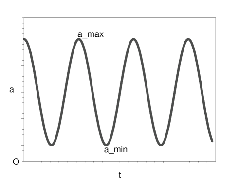
Figure 1: The evolution of the radius of the fluid sphere. This sphere oscillates between a maximum and a minimum radius and the classical singularity at $a=0$ is never reached.

In Fig. 1 we plot the evolution of the radius of the fluid sphere with $\rho=\rho_{f}/a^{f+2}$. The radius of the fluid sphere oscillates between a maximum $a_{\text{max}}=a_{0}$ and a minimum $a_{\text{min}}$ and the singularity does not form. The reason for this behavior can be understood as follows. According to the modified equation (11), the energy density continually increases as the sphere contracts, for as long as the $k$-term in the right hand side of this equation can be neglected. As the density approaches the critical density the collapse stops and, thereafter, the sphere begins to expand. As it reaches the maximum radius, the expansion stops and the sphere begins to collapse again.

The scenario described is the picture observed by a comoving observer. Since the singularity is not formed, the question arises of whether there is a black hole horizon or not. To answer this question, it is necessary to consider the frame of an observer located at spatial infinity.

3 Observer at spatial infinity

Here we extend the spacetime of Eq. (1) across the surface $\Sigma$ of the sphere and to spatial infinity. The angular coordinates $\theta$ and $\varphi$ are the same in both regions. Let us begin by rewriting the line element in different coordinates. By introducing the variable

$$r\equiv\frac{x}{a}\,,$$ (15)

the line element (1) becomes

$$ds^{2} = -\left(1-\frac{x^{2}H^{2}}{1-kr^{2}}\right)dt^{2}-\frac{2xH}{1-kr^{2}}\,dt\,dx$$ (16)

$$+\left(1-kr^{2}\right)^{-1}dx^{2}+x^{2}d\Omega_{(2)}^{2}\,,$$

where

$$H\equiv\frac{\dot{a}}{a}$$ (17)

is the usual Hubble parameter. In order to eliminate the cross-term $dt\,dx$ in the line element (16), we replace the comoving time $t$ with another time coordinate $\bar{t}$. To determine $\bar{t}$ we employ the “integrating factor method” [43], that is, we set

$$d\bar{t}=\eta^{-1}\left[-\left(1-\frac{x^{2}H^{2}}{1-kr^{2}}\right)dt-\frac{xH}{1-kr^{2}}\,dx\right]\,.$$ (18)

Here $\eta(t,\ x)$ is an integrating factor making $d\bar{t}$ a perfect differential, which is achieved if $\eta$ satisfies the equation

$$\partial_{x}\left[\eta^{-1}\left(1-\frac{x^{2}H^{2}}{1-kr^{2}}\right)\right]=\partial_{t}\left(\eta^{-1}\frac{xH}{1-kr^{2}}\right)\,.$$ (19)

The solution of this equation is

$$\eta=a^{2}H{F}\left(u\right)\;\ \ \ u\equiv\mbox{e}^{-2k{W}}\left(1-kr^{2}\right)\,$$

$${W}\equiv\int\frac{dt}{a^{2}H}\,$$ (20)

where ${F}(u)$ is an arbitrary function of $u$ (which makes it clear that the integrating factor is not unique). The line element (16) then becomes [44]

$$ds^{2} = -\eta^{2}\left(1-\frac{x^{2}H^{2}}{1-kr^{2}}\right)^{-1}d\bar{t}^{2}+x^{2}d\Omega_{(2)}^{2}$$ (21)

$$+\left(1-kr^{2}-x^{2}H^{2}\right)^{-1}dx^{2}\,.$$

By defining

$$F^{2}\equiv\eta^{2}\frac{1-kr^{2}}{\left(1-kr^{2}-x^{2}H^{2}\right)^{2}}\,,$$ (22)

it is

$$ds^{2} = -F^{2}\left[1-x^{2}\left(H^{2}+\frac{k}{a^{2}}\right)\right]d\bar{t}^{2}+x^{2}d\Omega_{(2)}^{2}$$ (23)

$$+\left[1-x^{2}\left(H^{2}+\frac{k}{a^{2}}\right)\right]^{-1}dx^{2}\,.$$

We now want to use the $\left(\bar{t},x,\theta,\varphi\right)$ coordinate system to extend the geometry determined by quantum gravity outside the fluid sphere. The resulting metric is interpreted as a quantum gravity geometry with a fluid also outside the surface $\Sigma$ of this sphere. If the matter density is much smaller than the Planck density, the quantum correction in Eq. (11) becomes negligible and the geometry reduces to a fluid solution of the Einstein equations. Using the modified Friedmann equation (11), the line element assumes the form

$$ds^{2} = -F^{2}\left[1-\frac{8\pi}{3}\rho\left(1-\frac{\rho}{\rho_{cr}}\right)x^{2}\right]d\bar{t}^{2}+x^{2}d\Omega_{(2)}^{2}$$ (24)

$$+\left[1-\frac{8\pi}{3}\rho\left(1-\frac{\rho}{\rho_{cr}}\right)x^{2}\right]^{-1}dx^{2}\,.$$

Using now the scaling of the perfect fluid density $\rho=\rho_{f}/a^{f+2}$, one obtains

$$ds^{2} = -F^{2}\left[1-\frac{8\pi}{3}\frac{\rho_{f}r^{f+2}}{x^{f}}\left(1-\frac{\rho_{f}r^{f+2}}{\rho_{cr}x^{f+2}}\right)\right]d\bar{t}^{2}$$ (25)

$$+\left[1-\frac{8\pi}{3}\frac{\rho_{f}r^{f+2}}{x^{f}}\left(1-\frac{\rho_{f}r^{f+2}}{\rho_{cr}x^{f+2}}\right)\right]^{-1}dx^{2}$$

$$+x^{2}d\Omega_{(2)}^{2}\,.$$

Here the metric components must be understood as functions of $\bar{t}$ and $x$ obtained by solving Eqs. (15), (18), (19), and (22). This metric continues the interior (FLRW) geometry of the fluid sphere across $\Sigma$ to the exterior and to spatial infinity, provided that suitable junction conditions (discussed below) are satisfied on $\Sigma$. In order to understand completely the behavior of the quantum-corrected fluid sphere, one should determine also the spacetime structure outside the sphere. What is this exterior geometry? Is it the Schwarzschild spacetime? The answer is no, for the following reason. At the surface $\Sigma$ (a timelike three-dimensional world tube which has the sphere as its intersection with any constant time slice), the exterior and interior geometries must match continuously [45]. According to the Israel junction conditions, if the match cannot be achieved, then there is a layer of material on the surface $\Sigma$ of the sphere. The relation between the jump of the stress-energy tensor at the surface and its intrinsic geometry is regulated by field equations (in general relativity, the jump of the Einstein tensor is proportional to the jump of the stress-energy tensor according to the Einstein equations) [46, 47]. In our case, however, no layer of material is present on $\Sigma$ and the minimal junction conditions required in any theory of gravity, that is continuous matching of induced 3-metrics and extrinsic curvatures, are imposed. We note that similar points are clarified in general terms in [48].

In the following we obtain the exterior spacetime using a “surface trick” (this method is described in Appendix A for general static and spherically symmetric spacetimes). We verify that the exterior geometry matches continuously the interior FLRW geometry at the surface of the fluid sphere.

At the surface of the sphere $r=r_{0}$ (where, since $r$ is a comoving coordinate, $r_{0}$ is a constant [45]), Eq. (25) yields

$$ds^{2} = -\left[1-\frac{2M_{f}}{x^{f}}\left(1-\frac{l^{f+2}}{x^{f+2}}\right)\right]d{\tilde{t}}^{2}+x^{2}d\Omega_{(2)}^{2}$$ (26)

$$+\left[1-\frac{2M_{f}}{x^{f}}\left(1-\frac{l^{f+2}}{x^{f+2}}\right)\right]^{-1}dx^{2}\,,$$

and

$$M_{f}\equiv\frac{4\pi}{3}\,\rho_{f}\,r_{0}^{f+2}\,,\ \ \ \ \ \ \ \ \ \ \ l^{f+2}\equiv\frac{\rho_{f}\,r_{0}^{f+2}}{\rho_{cr}}\,.$$ (27)

Here $\tilde{t}$ is defined as

$$\tilde{t}=\int F\left(\bar{t},\ r_{0}\right)d\bar{t}\,.$$ (28)

When $f=1$ (describing a pressureless dust), we recognize ${M}_{1}$ as the fluid energy enclosed by the sphere. The ${l}$-terms in the line element are generated by the LQC/braneworld correction. Eq. (26) describes a 2-parameter family of static and spherically symmetric spacetimes spanned by the parameters $M_{f}$ and $l$. When $f=1$ and $l\ll x$, Eq. (26) reduces to the Schwarzschild solution of the vacuum Einstein equations. At first glance, the metric (26) looks like a special case of the Kiselev metric [49], but differs from it in the sign and the $x$-dependence of the $l$-term.

Does the exterior metric (26) satisfy the Einstein equations outside the sphere? Clearly, it does not satisfy the vacuum Einstein equations because the Birkhoff theorem of general relativity guarantees that the unique vacuum, spherical, and asymptotically flat solution is the Schwarzschild one. Furthermore, the Schwarzschild metric can not match continuously the interior FLRW geometry for $f=2,4$, unless there is a layer of material on the surface of the sphere, which introduces some arbitrariness of choice that is best avoided. In order to match continuously exterior and interior geometry without matter layers on the surface $\Sigma$ of the sphere, the exterior solution must be given by Eq. (26). The interior FLRW geometry is not derived from the Einstein equations but from the braneworld modified Friedmann equation. Therefore, one should in principle construct the exterior solution from the equations of braneworld model. However, in general, one expects that $l/x\ll 1$ in the exterior and that the quantum correction ${(l/x)}^{f+2}$ can be safely neglected outside the sphere.

We note that, actually, considering the trace anomaly of quantum fluctuations, Abedi and Arfaei [50] have obtained the quantum corrected metric Eq. [26] for $f=1$.

The equation locating the apparent horizons (when they exist) is

$$1-\frac{2M_{f}}{x^{f}}\left(1-\frac{l^{f+2}}{x^{f+2}}\right)=0\,,$$ (29)

or

$$1-\frac{8\pi}{3}\frac{\rho_{f}\,r_{0}^{f+2}}{x^{f}}\left(1-\frac{\rho_{f}\,r_{0}^{f+2}}{\rho_{cr}\,x^{f+2}}\right)=0\,.$$ (30)

In general, this equation has two positive solutions, which means that there exist two apparent horizons with radii $x_{+}$ and $x_{-}$. $x_{+}$ denotes the outer apparent horizon, a surface of infinite redshift, while $x_{-}$ denotes an inner apparent horizon [51]. In particular, when $f=2$, then $x_{+}$ and $x_{-}$ can be expressed as

$$x_{+} = \left(\frac{2M_{2}}{3}\right)^{1/2}\Bigg{(}2\cos\mathfrak{s}+1\Bigg{)}^{1/2}\,,$$ (31)

$$x_{-} = \left(\frac{2M_{2}}{3}\right)^{1/2}\left[2\cos\left(\mathfrak{s}+\frac{4}{3}\pi\right)+1\right]^{1/2}\,,$$ (32)

where

$$\mathfrak{s}\equiv\frac{1}{3}\arccos\left({1-\frac{27l^{4}}{8M_{2}^{2}}}\right)\,.$$ (33)

When

$$1-\frac{27l^{4}}{16M_{2}^{2}}=0\;,$$ (34)

the two apparent horizons coincide. When $l^{4}\ll M_{2}^{2}$, then $x_{+}=\sqrt{2M_{2}}$ gives the outer horizon and $x_{-}=0$ gives the singularity. The causal structure of the exterior spacetime is similar to that of the Reissner-Nordström solution of the Einstein equations: the outer horizon is an apparent horizon, the inner apparent horizon resembles a Cauchy horizon [51], and the singularity is timelike. Therefore, the solution can also be used to describe a wormhole or Einstein-Rosen bridge connecting two asymptotically flat spacetimes.

Now a question arises: in the frame of an observer at spatial infinity, will the fluid sphere oscillate? Is the surface of this sphere inside or outside the apparent horizons? To answer these questions, we now turn to Eq. (11). Setting $\dot{a}=0$ in (11) yields the equation locating the critical radius of the fluid sphere:

$$1-\frac{8\pi}{3}\frac{\rho_{f}}{ka^{f}}\left(1-\frac{\rho_{f}}{\rho_{cr}a^{f+2}}\right)=0\,,$$ (35)

or

$$1-\frac{8\pi}{3}\left(\frac{r_{1}}{r_{0}}\right)^{2}\frac{\rho_{f}\,r_{0}^{f+2}}{x^{f}}\left(1-\frac{\rho_{f}\,r_{0}^{f+2}}{\rho_{cr}x^{f+2}}\right)=0\,,$$ (36)

where $k$ has the dimensions of the inverse of a squared length, hence we define

$$k\equiv\frac{1}{r_{1}^{2}}\,.$$ (37)

Eq. (36) provides two critical values of the radius $x$ (a proper length or areal radius), the maximum radius $x_{\text{max}}$ and the minimum radius $x_{\text{min}}$ of the fluid sphere. If $r_{1}=r_{0}$ we have

$$x_{\text{min}}=x_{-}\,,\ \ \ \ \ x_{\text{max}}=x_{+}\,,$$ (38)

which means that the minimum and maximum radii of the sphere coincide with those of the inner and outer apparent horizons, respectively.

If instead $r_{1}>r_{0}$ we have

$$x_{\text{min}}<x_{-}\,,\ \ \ \ \ x_{\text{max}}>x_{+}\,:$$ (39)

the fluid sphere can pulsate across the outer apparent horizon $x_{+}$ and the inner apparent horizon $x_{-}$.

If instead $r_{1}<r_{0}$ we get

$$x_{\text{min}}>x_{-}\,,\ \ \ \ \ x_{\text{max}}<x_{+}\,,$$ (40)

then the fluid sphere pulsates between the two apparent horizons $x_{+}$ and $x_{-}$. In this case the surface of infinite redshift $x_{+}$ conceals the sphere from the observer at infinity, who still sees a black hole.

We stress that the formation of an apparent horizon is not avoided since we always have $x_{\text{min}}<x_{+}$. Secondly, the pulsation of the sphere between minimum and maximum radii is experienced by the comoving observer but not by the observer at infinity, for whom the sphere will take an infinite time to reach the outer apparent horizon. Therefore, the pulsation of the sphere is completely unobservable by the observer at infinity. In Fig. 2 we plot the variation of proper time $t$ for the comoving observer and the Schwarzschild time $\tilde{t}$ for the observer at infinity during the process of collapse (or pulsation) of the sphere.The variation of the sphere surface with the proper time $t$ and the Schwarzschild time $\tilde{t}$ are determined by Eq. (49) and

$$\frac{dR}{d\tilde{t}} = -\frac{E}{\sqrt{E^{2}-\left[1-\frac{2M_{f}}{R^{f}}\left(1-\frac{l^{f+2}}{R^{f+2}}\right)\right]}}$$ (41)

$$\cdot\left[1-\frac{2M_{f}}{R^{f}}\left(1-\frac{l^{f+2}}{R^{f+2}}\right)\right]\,,$$

respectively.

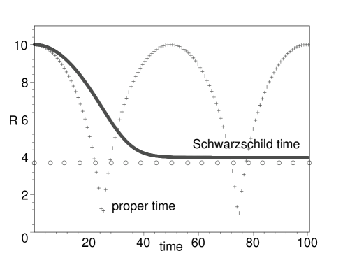
Figure 2: The variation of the sphere surface with the proper time $t$ and Schwarzschild time $\tilde{t}$, starting at rest at $R_{0}=10$ and falling toward the center (for the parameter values $f=1$, $M_{1}=2$, $l=0.79$, and $E=0.77$).

For realistic astrophysical objects and the case $f=1$, Eq. (36) can be safely approximated by

$$\left(\frac{r_{0}}{r_{1}}\right)^{2}=\frac{2M_{1}}{x}\,.$$ (42)

The right hand side of Eq. (42) is twice the negative of the Newtonian potential $-M_{1}/x$. In general, we have

$$\frac{2M_{1}}{x}\ll 1$$ (43)

and

$$r_{0}\ll r_{1}\,.$$ (44)

In this case the fluid sphere can oscillate across the outer horizon $x_{+}$. But for the observer at infinity, it takes an infinite time for the sphere to cross this horizon. The case $r_{1}<r_{0}$ is interesting: in this case the fluid sphere oscillates inside the outer horizon $x_{+}$, behaving as a quantum “beating heart” of the black hole. To summarize, the black hole singularity is now replaced by a pulsating sphere, the pulsation of which is completely unobservable by an observer at infinity.

We remind the reader that the density distribution within the sphere $r_{0}$ is assumed to be perfectly spherical. In reality, this density distribution could be asymmetric and the quadrupole moment be time-dependent. Then, presumably, the energy loss due to gravitational wave radiation (if still applicable) would damp the oscillation and the beating of the “quantum heart”, and lead to $a_{\rm max}\rightarrow a_{\rm min}$.

In the next section we discuss the matching between exterior and interior geometries at the surface of the fluid sphere.

4 Matching interior and exterior geometries

The field equations are satisfied on the surface of the sphere if and only if the induced 3-metrics and extrinsic curvatures of the surface’s three-dimensional world tube are the same, whether measured from its interior or from its exterior. In this section we verify that this is indeed the case for the oscillating sphere discussed above.

The surface of the sphere has constant radial coordinate $r=r_{0}$. Eq. (1) gives the proper circumferential radius of the sphere $R(t)=a(t)\,r_{0}$, where $a(t)$ obeys Eq. (11). Assuming that the fluid is initially at rest at time $t=0$, it is $a(0)=a_{0}$, $\dot{a}(0)=0$ and

$$k=\frac{8\pi}{3}\frac{\rho_{f}}{a_{0}^{f}}\left(1-\frac{\rho_{f}}{\rho_{cr}\,a_{0}^{f+2}}\right)\,.$$ (45)

Eq. (11) then assumes the form

$$\dot{a}^{2}=\frac{8\pi}{3}\left[\frac{\rho_{f}}{a^{f}}\left(1-\frac{\rho_{f}}{\rho_{cr}a^{f+2}}\right)-\frac{\rho_{f}}{a_{0}^{f}}\left(1-\frac{\rho_{f}}{\rho_{cr}\,a_{0}^{f+2}}\right)\right]\,.$$ (46)

Once $a(t)$ is derived from Eq. (46), the intrinsic 3-metric induced on the surface $\Sigma$ of the sphere, as measured from the FLRW interior, is obtained by setting $r=r_{0}$ in Eq. (1):

$$ds^{2}_{(-)}=-dt^{2}+a^{2}r_{0}^{2}d\Omega_{(2)}^{2}\,.$$ (47)

Let us focus now on the exterior metric (26). The surface of the sphere is at coordinate

$$x=R\left({t}\right)=a(t)\,r_{0}\,,$$ (48)

and $t$ is the proper time of this surface. The 4-velocity $v^{a}$ of this surface is tangent to its spacetime trajectory, which is a timelike curve and, therefore, satisfies $v^{c}v_{c}=-1$. This normalization determines $R({t})$ through

$$\dot{R}^{2}=E^{2}-\left[1-\frac{2M_{f}}{R^{f}}\left(1-\frac{l^{f+2}}{R^{f+2}}\right)\right]\,.$$ (49)

At $t=0$ and $R=R_{0}=a_{0}r_{0}$, the radial velocity of the surface vanishes, $dR/dt=0$, which gives

$$E^{2}=1-\frac{2M_{f}}{R^{f}_{0}}\left(1-\frac{l^{f+2}}{R^{f+2}_{0}}\right)\,.$$ (50)

Eq. (49) then takes the form

$$\dot{R}^{2}=\frac{2M_{f}}{R^{f}}\left(1-\frac{l^{f+2}}{R^{f+2}}\right)-\frac{2M_{f}}{R^{f}_{0}}\left(1-\frac{l^{f+2}}{R^{f+2}_{0}}\right)\,.$$ (51)

Eqs. (46) and (51) agree if and only if

$$R=ar_{0}\,,\ \ \ \ \ R_{0}=a_{0}r_{0}\,.$$ (52)

Substituting $x=R$ with Eq. (49) and Eq. (52) into the exterior solution (26), we find the line element on the surface to be

$$ds_{(+)}^{2} = -\left[1-\frac{2M_{f}}{R^{f}}\left(1-\frac{l^{f+2}}{R^{f+2}}\right)\right]\left(\frac{d\tilde{t}}{dt}\right)^{2}dt^{2}+R^{2}d\Omega^{2}_{(2)}$$ (53)

$$+\left[1-\frac{2M_{f}}{R^{f}}\left(1-\frac{l^{f+2}}{R^{f+2}}\right)\right]^{-1}\left(\frac{dR}{dt}\right)^{2}dt^{2}\,$$

$$= -\left[1-\frac{2M_{f}}{R^{f}}\left(1-\frac{l^{f+2}}{R^{f+2}}\right)\right]^{-1}E^{2}dt^{2}+R^{2}d\Omega_{(2)}^{2}$$

$$+\left[1-\frac{2M_{f}}{R^{f}}\left(1-\frac{l^{f+2}}{R^{f+2}}\right)\right]^{-1}\left(\frac{dR}{dt}\right)^{2}dt^{2}$$

$$= -dt^{2}+a^{2}r_{0}^{2}d\Omega_{(2)}^{2}\,,$$

which is exactly the 3-metric (46) as measured from the FLRW interior of the sphere. Therefore, the 3-metrics induced by the exterior and interior 4-dimensional metrics match continuously on the surface of the sphere.

Let us consider now the extrinsic curvatures of both interior and exterior. It is necessary and sufficient to show that the extrinsic curvatures $K_{ij}$ of the surface are the same whether measured in the exterior or the interior. First, we calculate $K_{ij}^{(-)}$ in the FLRW interior. Since $t$ is the proper time on the surface $\Sigma$, the components of its 4-velocity in coordinates $\left(\tilde{t},x,\theta,\varphi\right)$ are

$$v^{\mu} = \frac{dx^{\mu}}{dt}=\left(\frac{d\tilde{t}}{dt},\frac{dR}{dt},0,0\right)$$ (54)

$$= \left(\frac{E}{1-\frac{2M_{f}}{R^{f}}\left(1-\frac{l^{f+2}}{R^{f+2}}\right)},\dot{R},0,0\right)\,.$$

The normal vector to $\Sigma$ is

$$n^{a}=\frac{\sqrt{1-kr_{0}^{2}}}{a}\left(\frac{\partial}{\partial r}\right)^{a}\,,$$ (55)

while the vectors $v^{a}=\left(\partial/\partial t\right)^{a},\ \left(\partial/\partial\theta\right)^{a}$, and $\left(\partial/\partial\phi\right)^{a}$ lie in the surface. Let the indices $i$ and $j$ run over $t,\ \theta$, and $\phi$. Then we have

$$K_{ij}^{(-)}\equiv e_{(i)}^{a}e_{(j)}^{b}\nabla_{a}n_{b}=\frac{1}{2}\,\pounds_{n}g_{ij}\,,$$ (56)

where $\left\{e^{a}_{(t)},e^{a}_{(\theta)},e^{a}_{(\varphi)}\right\}=\left\{e^{a}_{(i)}\right\}$ is a triad of vectors on the surface of the sphere, the subscript $(i)$ denotes a triad index, and $\pounds_{n}$ is the Lie derivative along the direction of the unit normal $n^{a}$. The metric (1) gives

$$K_{tt}^{(-)}=K_{t\theta}^{(-)}=K_{t\phi}^{(-)}=K_{\theta\phi}^{(-)}=0\,,$$ (57)

$$K_{\theta\theta}^{(-)}=K_{\phi\phi}^{(-)}\sin^{-2}\theta=ar_{0}\sqrt{1-kr_{0}^{2}}\,.$$ (58)

We then calculate the extrinsic curvature $K_{ij}^{(+)}$ in the exterior region. In the background of the exterior spacetime (26), the 4-velocity of the spherical surface is

$$v^{a}=v^{\tilde{t}}e_{(\tilde{t})}^{a}+v^{x}e_{(x)}^{a}\,.$$ (59)

The normal vector is

$$n^{a}=n^{\tilde{t}}e_{(\tilde{t})}^{a}+n^{x}e_{(x)}^{a}\,.$$ (60)

These vectors satisfy the conditions

$$n^{c}n_{c}=1\,,\ \ \ n^{c}v_{c}=0\,,\ \ \ v^{c}v_{c}=-1\,,$$ (61)

from which one obtains also

$$n^{\tilde{t}}=v_{x}\,,\ \ \ n^{x}=-v_{\tilde{t}}\,.$$ (62)

Let $i$ and $j$ run over the values $t,\ \theta$, and $\phi$ as before, then Eq. (56) holds for the exterior metric, with

$$e_{(\tilde{t})}^{c}e^{(\tilde{t})}_{c} = v^{c}v_{c}=-1\,,$$ (63)

$$e_{(\tilde{t})}^{c}e^{(\theta)}_{c} = e_{(\tilde{t})}^{c}e^{(\phi)}_{c}=e_{(\theta)}^{c}e^{(\phi)}_{c}=0\,.$$ (64)

We have

$$K_{{t}{t}}^{(+)}=K_{{t}\theta}^{(+)}=K_{{t}\phi}^{(+)}=K_{\theta\phi}^{(+)}=0\;,$$ (65)

and

$$K_{\theta\theta}^{(+)}=K_{\phi\phi}^{(+)}\sin^{-2}\theta=\frac{1}{2}\left(x^{2}\right)_{,n}$$

$$=\frac{1}{2}\left(x^{2}\right)_{,x}n^{x}=-xv_{\tilde{t}}=RE$$

$$=R\left[1-\frac{2M_{f}}{R^{f}_{0}}\left(1-\frac{l^{f+2}}{R^{f+2}_{0}}\right)\right]^{1/2}$$

$$=ar_{0}\sqrt{1-kr_{0}^{2}}\,,$$ (66)

where we used Eqs. (47), (52), and

$$v^{\tilde{t}}=\frac{d\tilde{t}}{dt}=\frac{\left[1-\frac{2M_{f}}{R^{f}_{0}}\left(1-\frac{l^{f+2}}{R^{f+2}_{0}}\right)\right]^{\frac{1}{2}}}{1-\frac{2M_{f}}{R^{f}}\left(1-\frac{l^{f+2}}{R^{f+2}}\right)}\,.$$ (67)

Therefore, it is

$$K_{ij}^{(-)}=K_{ij}^{(+)}\,,$$ (68)

which completes the proof.

5 Discussion and conclusions

The Hawking-Penrose singularity theorem, based on general relativity, dictates that there is a singularity at the center of a black hole. In order to remove this singularity, one must resort to a more fundamental quantum theory of gravity. We currently have two main contenders to the role of such a theory, LQG and string theory. Using the dynamical equation arising in LQC or braneworld models, we have studied the gravitational collapse of a perfect fluid sphere. Within the context of LQC, note here that an approximation to the full effective dynamics is adopted in the present work. This approximation underlies the replacement of the full Eq. (12) with Eq. (11) at the beginning of our discussion.

We find that, in the comoving frame, the sphere does not collapse to a singularity but pulsates instead between a maximum and a minimum size, effectively removing the singularity from the gravitational collapse. In the process of seeking the solution exterior to the sphere, we propose a method for constructing the exterior solution. We then find that the exterior solution usually has two horizons, which is reminiscent of the Reissner-Nordström black hole spacetime of classical relativity. As a result, in the frame of an observer at spatial infinity, the collapsing fluid takes an infinite coordinate time to cross the outer horizon and the pulsations of the quantum-corrected core are completely unobservable by the far-away observer. Borrowing current terminology from black hole astrophysics, the pulsating core hidden inside the apparent horizon plays the role of a “beating heart” for the black hole.

Appendix A From interior to exterior solution

Here we show how to obtain the exterior solution from the interior one using our “surface trick” in the context of general relativity.

The metric for a homogenous and isotropic fluid sphere is given by Eq. (1), where the scale factor $a$ obeys Eq. (2). Following the procedure of Sec. 3, we rewrite Eq. (1) in the frame of the observer at infinity as

$$ds^{2} = -F^{2}\left(1-\frac{8\pi}{3}\rho x^{2}\right)d\bar{t}^{2}+x^{2}d\Omega_{(2)}^{2}$$ (69)

$$+\left(1-\frac{8\pi}{3}\rho x^{2}\right)^{-1}dx^{2}\,,$$

where the metric components must be understood as functions of $\bar{t}$ and $x$.

At the surface $r=r_{0}$ of the sphere ($r_{0}$ is a constant, since $r$ is a comoving coordinate [45]), we have

$$ds^{2} = -\left[1-\frac{8\pi}{3}\rho\left(\frac{x}{r_{0}}\right)x^{2}\right]d\tilde{t}^{2}+x^{2}d\Omega_{(2)}^{2}$$ (70)

$$+\left[1-\frac{8\pi}{3}\rho\left(\frac{x}{r_{0}}\right)x^{2}\right]^{-1}dx^{2}\,.$$

The metric (70) also represents the exterior metric at the surface $r=r_{0}$. Thus we can take this static spherically symmetric spacetime as the exterior solution of the fluid sphere. Similar to the proof in Sec. 4, we can show that the exterior geometry (70) matches continuously the interior one (1).

As an example, we consider the energy density

$$\rho=\lambda+\frac{\rho_{m}}{a^{3}}+\frac{\rho_{r}}{a^{4}}\,,$$ (71)

with $\lambda$ for the cosmological constant energy density, ${\rho_{m}}/{a^{3}}$ for the dust density, and ${\rho_{r}}/{a^{4}}$ for the radiation density. Substituting Eq. (71) with $a=x/r_{0}$ into Eq. (70), one obtains

$$ds^{2} = -\left(1-\frac{2M}{x}-\frac{Q^{2}}{x^{2}}-\Lambda x^{2}\right)d\tilde{t}^{2}+x^{2}d\Omega_{(2)}^{2}$$ (72)

$$+\left(1-\frac{2M}{x}-\frac{Q^{2}}{x^{2}}-\Lambda x^{2}\right)^{-1}dx^{2}\,,$$

where

$$M\equiv\frac{4\pi}{3}\rho_{m}r_{0}^{3}\,,\ \ \ \ \ Q^{2}\equiv\frac{8\pi}{3}\rho_{r}r_{0}^{4}\,,\ \ \ \ \ \Lambda\equiv\frac{8\pi}{3}\lambda\,.$$ (73)

The metric (72) is the Reissner-Nordström-de Sitter solution of the Einstein equations with the formal replacement $Q\rightarrow iQ$. While $M$ plays the role of a mass, $Q^{2}$ also plays the role of the mass of radiation (not of electric charge) contained in a sphere. In fact, the thermal bath of radiation with density $\rho_{r}/a^{4}$ has nothing to do with free electric charges and the analogy with Reissner-Nordström-de Sitter is purely formal and not complete (because of the opposite sign of the term in $Q^{2}/x^{2}$).

Appendix B From exterior to interior solution

Here we show how to obtain the interior geometry from the exterior one in the context of general relativity. We focus on the static spherically symmetric spacetime

$$ds^{2} = -\left[1-\frac{8\pi}{3}\rho\left(x\right)x^{2}\right]d\tilde{t}^{2}+x^{2}d\Omega_{(2)}^{2}$$ (74)

$$+\left[1-\frac{8\pi}{3}\rho\left(x\right)x^{2}\right]^{-1}dx^{2}\,.$$

We assume that the spacetime exterior to a perfect fluid sphere is given by Eq. (74). Then our task is to look for the interior solution starting from this exterior. The normalization of the tangent $v^{a}$ to the trajectory described by the surface of the sphere in spacetime gives

$$\dot{x}^{2}=E^{2}-1+\frac{8\pi}{3}\rho x^{2}\,,$$ (75)

with an overdot denoting differentiation with respect to the proper time $t$ and where $E$ is an integration constant. Eqs. (75) and (2) coincide provided that

$$x=ar_{0}\,\ \ \ \ \ \ -kr_{0}^{2}=E^{2}-1\,,$$ (76)

with $r_{0}$ a constant. This coincidence motivates us to consider simply the homogenous and isotropic perfect fluid sphere as the interior solution. Then $\rho$ plays the role of the energy density in the comoving frame. We have checked that the resulting interior solution does match the exterior solution continuously. In the following we consider, as an example, the Bardeen metric [52] as the exterior geometry outside a perfect fluid sphere.

The Bardeen line element describing a regular black hole is

$$ds^{2} = -\left[1-\frac{2Mx^{2}}{\left(x^{2}+q^{2}\right)^{3/2}}\right]d\tilde{t}^{2}+x^{2}d\Omega_{(2)}^{2}$$ (77)

$$+\left[1-\frac{2Mx^{2}}{\left(x^{2}+q^{2}\right)^{3/2}}\right]^{-1}dx^{2}\,,$$

where $M$ is the mass and $q$ is the monopole charge of a self-gravitating magnetic field described by a nonlinear electrodynamics [53]. This model has been revisited by Borde, who clarified the avoidance of singularities in this spacetime [54, 55]. For a certain range of the parameter $q$, the Bardeen metric describes a black hole. When $x\gg q$, it behaves as the Schwarzschild black hole but, when $x\ll q$, it behaves as de Sitter space, therefore, the spacetime in general has two apparent horizons. Explicitly, there are two such horizons when

$$|q|<\frac{4M}{3\sqrt{3}}\,.$$ (78)

Given the exterior metric (77), one can read off the corresponding energy density of the perfect fluid sphere, which can be parameterized as

$$\rho = \frac{\rho_{m}}{\left(a^{2}+a_{0}^{2}\right)^{3/2}}\,,$$ (79)

where $\rho_{m}$ and $a_{0}$ are two constants and $a(t)$ is the time-dependent radius of the fluid sphere. Substituting Eq. (79) into Eq. (2) yields

$${\dot{a}^{2}}=\frac{8\pi}{3}\frac{\rho_{m}a^{2}}{\left(a^{2}+a_{0}^{2}\right)^{3/2}}-k\,,$$ (80)

describing a pulsating sphere. However, the pulsation is again unobservable by an observer at infinity due to the unavoidable formation of an apparent horizon. On the other hand, if we regard the above equation as the Friedmann equation to study its cosmic evolution, we find it can give an exponential inflationary universe provided that $a\ll a_{0}$. Thus it would be interesting to investigate this inflationary model in great detail.

References

- [1] S.W. Hawking and R. Penrose, Proc. Roy. Soc. Lond. A 314, 529 (1970).
- [2] J.H. Schwarz, in Measuring and Modeling the Universe, Proceedings, Pasadena, USA, November 17-22, 2002 W.L. Freedman ed. (Cambridge University Press, Cambridge, UK 2004), pp. 53-66 [arXiv:astro-ph/0304507].
- [3] See, e.g., A. Ashtekar and J. Lewandowski, Class. Quantum Grav. 21, R53 (2004).
- [4] J.R. Oppenheimer and H. Snyder, Phys. Rev. D 56, 455 (1939).
- [5] A. Ashtekar, S. Fairhurst, and J.L. Willis, Class. Quantum Grav. 20, 1031 (2003).
- [6] C.G. Boehmer and K. Vandersloot, Phys. Rev. D 76, 104030 (2007) [arXiv:0709.2129].
- [7] L. Modesto, Class. Quantum Grav. 23, 5587 (2006) [arXiv:gr-qc/0509078].
- [8] A. Corichi and P. Singh, Class. Quantum Grav. 33, 055006 (2016) [arXiv:gr-qc/1506.08015].
- [9] J. Olmedo, S. Saini, and P. Singh, arXiv:gr-qc/1707.07333.
- [10] M. Campiglia, R. Gambini, and J. Pullin, Class. Quantum Grav. 24, 3649 (2007) [arXiv:gr-qc/0703135].
- [11] M. Bojowald, R. Goswami, R. Maartens, and P. Singh, Phys. Rev. Lett. 95, 091302 (2005).
- [12] L. Modesto, Adv. High Energy Phys. 2008, 459290 (2008).
- [13] D.W. Chiou, Phys. Rev. D 78, 064040 (2008) [arXiv:gr-qc/0611043].
- [14] M. Bojowald, T. Harada, and R. Tibrewala, Phys. Rev. D 78, 064057 (2008).
- [15] G. Rodolfo and J. Pullin, Phys. Rev. Lett. 101, 161301 (2008).
- [16] B.K. Tippett and V. Husain, Phys. Rev. D 84, 104031 (2011).
- [17] L. Modesto, Phys. Rev. D 70, 124009 (2004).
- [18] J. Ziprick and G. Kunstatter, Phys. Rev. D 80, 024032 (2009).
- [19] A. Peltola and G. Kunstatter, Phys. Rev. D 80, 044031 (2009).
- [20] C. Bambi, D. Malafarina, and L. Modesto, Phys. Rev. D 88, 044009(2013).
- [21] Y. Liu, D. Malafarina, L. Modesto, and C. Bambi, Phys. Rev. D 90, 044040 (2014).
- [22] D. Malafarina, Universe 3, 48 (2017).
- [23] R.M. Wald, General Relativity (Chicago University Press, Chicago, 1984).
- [24] S.W. Hawking and G.F.R. Ellis, The Large Scale Structure of Space-Time (Cambridge University Press, Cambridge, UK 1973), p. 135.
- [25] G. Vereshchagin, JCAP 0407, 013 (2004) [arXiv:gr-qc/0406108].
- [26] P. Singh, K. Vandersloot, and G. Vereshchagin, Phys. Rev. D 74, 043510 (2006) [arXiv:gr-qc/0606032].
- [27] A. Ashtekar, T. Pawlowski, P. Singh, and K. Vandersloot, Phys. Rev. D 75, 024035 (2007) [arXiv:gr-qc/0612104].
- [28] P. Singh and F. Vidotto, Phys. Rev. D 83, 064027 (2011) [arXiv:gr-qc/1012.1307].
- [29] J. L. Dupuy and P. Singh, Phys. Rev. D 95, 023510 (2017) [arXiv:gr-qc/1608.07772].
- [30] A. Ashtekar, T. Pawlowski, and P. Singh, Phys. Rev. D 74, 084003 (2006) [arXiv:gr-qc/0607039].
- [31] P. Diener, B. Gupt and P. Singh, Class. Quantum Grav. 31, 105015 (2014) [arXiv:gr-qc/1402.6613].
- [32] A. Ashtekar, T. Pawlowski, and P. Singh, Phys. Rev. Lett. 96, 141301 (2006) [arXiv:gr-qc/0602086].
- [33] E. Wilson-Ewing, JCAP 1303, 026 (2013) [arXiv:1211.6269].
- [34] M. Bojowald, Quantum Cosmology (Springer, New York, 2011).
- [35] Y. Shtanov and V. Sahni, Phys. Lett. B 557, 1 (2003) [arXiv:gr-qc/0208047].
- [36] M. Seikel and M. Camenzind, Phys. Rev. D 79, 083531 (2009) [arXiv:astro-ph/0811.4629].
- [37] M.G. Brown, K. Freese, and W.H. Kinney, JCAP 0803, 002 (2008) [arXiv:astro-ph/0405353].
- [38] A. Ashtekar, AIP Conf. Proc. 861, 3 (2006) [arXiv:gr-qc/0605011].
- [39] G. J. Olmo and P. Singh, JCAP 0901, 030 (2009) [arXiv:gr-qc/0806.2783].
- [40] A. Corichi and E. Montoya, Phys. Rev. D 84, 044021 (2011).
- [41] P. Diener, B. Gupt, M. Megevand, and P. Singh, Class. Quantum Grav. 31, 165006 (2014) [arXiv:hep-ph/1406.1486].
- [42] C. Rovelli and E. Wilson-Ewing, Phys. Rev. D 90, 023538 (2014).
- [43] S. Weinberg, Gravitation and Cosmology (Wiley, New York, 1972).
- [44] R. Y. Yu and T. Wang, Pramana. 80, 349 (2013); T. Wang, Class. Quantum Grav. 32, 195006 (2015).
- [45] C.W. Misner, K.S. Thorne, and J.A. Wheeler, Gravitation (San Francisco, Freeman, 1973).
- [46] W. Israel, Nuovo Cimento B 44, 1 (1966); Erratum 48, 463 (1967).
- [47] E. Poisson, A Relativist’s Toolkit (Cambridge University Press, Cambridge, UK 2004).
- [48] C. Barceló, R. Carballo-Rubio, and L. J. Garay, Universe 2, 7 (2016).
- [49] V.V. Kiselev, Class. Quantum Grav. 20, 1187 (2003).
- [50] J. Abedi and H. Arfaei, JHEP. 03, 135 (2016).
- [51] P. Chen, Y. C. Ong, and D.-h. Yeom, Phys. Rep. 603, 1 (2015).
- [52] J.M. Bardeen, in Conference Proceedings of GR5 (Tbilisi, USSR, 1968), p. 174.
- [53] E. Ayón-Beato and A. Garcia, Phys. Lett. B 493, 149 (2000).
- [54] A. Borde, Phys. Rev. D 50, 3392 (1994).
- [55] A. Borde, Phys. Rev. D 55, 7615 (1997).