A Regress-Later Algorithm for Backward Stochastic Differential Equations

Abstract

This work deals with the numerical approximation of backward stochastic differential equations (BSDEs). We propose a new algorithm which is based on the regression-later approach and the least squares Monte Carlo method. We give some conditions under which our numerical algorithm convergences and solve two practical experiments to illustrate its performance.

Keywords: BSDE, SDE, PDE, Regression, Monte Carlo, Pricing.

1 Introduction

This work deals with the numerical approximation of backward stochastic differential equations (BSDEs) on a certain time interval $[0,T]$. Backward stochastic differential equations were first introduced by Bismut [7] in the linear case and later developed by Pardoux and Peng [36]. In the past decade, BSDEs have attracted a lot of attention and have been intensively studied in mathematical finance, insurance and stochastic optimal control theory. For example in a complete financial market, the price of a standard European option can be seen as the solution of a linear BSDE. Moreover, the price of an American option can be formulated as the solution of a reflected BSDE.

BSDEs have also been widely applied for portfolio optimization, indifference pricing, modelling of convex risk measures and the modelling of ambiguity with respect to the stochastic drift and the volatility. See for instance El Karoui et al. [19], Cheridito et al. [13], Barles et al. [4], Duffie et al. [17], Hamadène et al. [25], Hu et al. [26], Leaven and Stadje [31] and the references therein. In general, many of these equations do not have an explicit or closed form solution. Due to its importance, some efforts have been made to provide numerical solutions. A four-step scheme has been proposed for instance by Ma et al. in [32] to solve forward-backward stochastic differential equations (FBSDEs). In [3], Bally has proposed a random time discretization scheme. Discrete time approximation schemes have also been proposed by Bouchard and Touzi in [8] and Chevance [14] for instance. In Chevance’s work [14], strong regularity assumptions of the coefficients of the BSDE are requiered for the convergence results. In Crisan et al. [15], was proposed a cubature techniques for BSDEs with application to nonlinear pricing. Gobet et al. [22] presented a discrete algorithm based on the Monte Carlo method to solve BSDEs. Recently, Fourier methods to solve FBSDEs were proposed by Huijskens et al. [27] and a convolution method by Hyndman et al. [28]. Briand et al. [9] proposed an algorithm to solve BSDEs based on Wiener chaos and Picard’s iterations expansion. Gobet et al. [23] designed a numerical scheme for solving BSDEs with using Malliavin weights and least-squares regression. Reducing variance in numerical solution of BSDEs is proposed by Alanko et al. [1]. Other recent references can be found in Chassagneux et al. [12], Khedher et al. [30], Bender et al. [5], Zhao et al. [40], Ventura et al. [38], Gong et al. [24], among others.

We propose in this paper a new algorithm which is based on a regression-later approach. Glasserman and Ye [20] show that the regression-later approach offers advantages in comparison to the classical regression technique. An asymptotic convergence rate of the regression-later technique is derived under some mild auxiliary assumption in Beutner et al. [6] for single-period problems. Stentohoff [37] discusses the convergence of the regression-now (cf. [20]) technique in the case of the evaluation of an American option.

Under some regularity assumptions, the solution of a FBSDE can be represented by the solution of a regular semi-linear parabolic partial differential equation (PDE). By exploiting the Markov property of the solution of the FBSDE, we have developed a probabilistic numerical regression called regression-later algorithm based on the least squares Monte Carlo method and the previous connection between the quasi-linear parabolic partial differential equation and the FBSDE. To the best of our knowledge, the regression-later approach has not been already used in the BSDE literature. For most numerical algorithms to solve BSDEs, we need to compute in general two conditional expectations at each step across the time interval. This computation can be very costly especially in high dimensional problems. For most numerical algorithms, it is important to note that the process $Z$ is more difficult to compute than the process $Y$. The proposed algorithm requires only one conditional expectation to compute at each step across the time interval. The algorithm yields good convergence results in practice and the computation of $Z$ is simple.

This paper is structured as follows. In the first part of our work, we introduce the basic theory of BSDEs, give some general results on the studies of FBSDEs and review the classical backward Euler-Maruyama scheme.

In the next step, we describe in detail the regression-later algorithm and derive a convergence result of the scheme. Finally, we provide two numerical experiments to illustrate the performance of the regression-later algorithm: the first in the context of option pricing and the second discusses the case where the forward process is a Wiener process.

Notations and Assumptions

We will use in this chapter the notations of El Karoui et al. [18]. We consider a filtered probability space $(\Omega,\mathcal{F},\mathbb{P},\mathbb{F})$ with $\mathcal{F}=\mathcal{F}_{T}$, $\mathbb{F}=(\mathcal{F}_{t})_{0\leq t\leq T}$ a complete natural filtration of a $d$-dimensional Brownian motion $W$ and $T$ a fixed finite horizon. For all $m\in\mathbb{N}^{*}$ and $x\in\mathbb{R}^{m}$, $|x|$ denotes the Euclidean norm of $x$. For the matrix $A\in\mathbb{R}^{m\times d}$, we define its Frobenius norm by $|A|:=\sqrt{\text{Trace}(AA^{*})}$. The matrix $A$ can be considered as an element of the space $\mathbb{R}^{m\times d}$.

• $\mathbb{L}^{2}_{m}(\mathcal{F}_{t}):=\bigg{\{}(X_{t})_{t\in[0,T]}\in\mathbb{R}^{m},\,\mathcal{F}_{t}-\text{measurable and}$

  $$\left\|X\right\|_{\mathbb{L}^{2}}=\mathbb{E}[\left|X_{t}\right|^{2}]^{1/2}<\infty\bigg{\}}.$$

• $\mathcal{S}^{2}(\mathbb{R}^{m}):=\bigg{\{}(Y_{t})_{t\in[0,T]}\in\mathbb{R}^{m},\,\text{continuous and adapted such that}$

  $${\displaystyle\left\|Y\right\|_{\mathcal{S}^{2}}^{2}=\mathbb{E}[\sup_{t\in[0,T]}\left|Y_{t}\right|^{2}]<\infty\bigg{\}}}.$$

• $\mathcal{H}^{2}(\mathbb{R}^{m}):=\bigg{\{}(Z_{t})_{t\in[0,T]}\in\mathbb{R}^{m},\,\text{continuous and adapted such that}$

  $${{\left\|Z\right\|_{\mathcal{H}^{2}}^{2}=\mathbb{E}[(\int_{0}^{T}\left|Z_{s}\right|^{2}ds)]<\infty\bigg{\}}}}.$$

• All the equalities and the inequalities between random variables are understood in almost sure sense unless explicitly stated otherwise.

• $\mathcal{C}^{l,k}_{b}([0,T]\times\mathbb{R}^{m})$ is the set of real valued functions which are $l$ times continuously differentiable in their first coordinate and $k$ times in their second coordinate with bounded partial derivatives up to order $k$.

• $\mathcal{C}^{k}(\Omega)$ is the set of $k$ times continuously differentiable functions on $\Omega$.

• For $x\in\mathbb{R}^{m}$, $\nabla_{x}:=(\frac{\partial}{\partial x_{1}},\cdots,\frac{\partial}{\partial x_{m}})$. The operator $\nabla_{x}$ is called the gradient. In the one-dimensional case, we will use the same notation.

• For $x,y\in\mathbb{R}^{m}$, $x.y$ denotes the usual inner product on the space $\mathbb{R}^{m}$.

2 Definitions and Estimates

In this section, we introduce the general concept of backward stochastic differential equations and forward-backward stochastic differential equations with respect to the standard Brownian motion. In the last part of the section, we recall some classical estimates from the theory of BSDEs.

2.1 Backward Stochastic Differential Equations

In the filtered probability space $(\Omega,\mathcal{F},\mathbb{P},\mathbb{F})$, backward stochastic differential equations are a special class of stochastic differential equations. The main difference is that these equations are specified with a prescribed terminal value as shown in the following equation

$$\left\{\begin{aligned} -&dY_{t}=f(t,Y_{t},Z_{t})dt-Z_{t}dW_{t};\qquad 0\leq t<T,\\ &Y_{T}=\xi.\end{aligned}\right.$$ (2.1)

The preceding system can be written equivalently as the following

$$\left.\begin{aligned} Y_{t}=\xi+\int_{t}^{T}f(s,Y_{s},Z_{s})ds-\int_{t}^{T}Z_{s}dW_{s},\\ \end{aligned}\right.$$ (2.2)

where

• $\xi$ is the terminal condition of the equation (2.1) and is assumed to be an $\mathcal{F}_{T}$- measurable and a square integrable random variable,

• the measurable mapping $(t,y,z)\mapsto f(t,y,z)$ is generally called the generator of (2.1).

A solution of the backward stochastic differential equation  (2.1) is a couple of progressively measurable processes $(Y,Z)$ such that:

$$\left\{\begin{aligned} &i)\quad\int_{0}^{T}|Z_{s}|^{2}ds<\infty\text{ and }\int_{0}^{T}\left|f(s,Y_{s},Z_{s})\right|ds<\infty,\\ &ii)\quad(Y_{t},Z_{t})\quad\text{satisfies the equation}~{}\eqref{art1_EDSR00},\end{aligned}\right.$$

In general, the equation (2.1) does not admit a unique solution. The existence and uniqueness of a solution can be shown under the conditions given in Pardoux and Peng [35] which involves the Lipschitz continuity of the driver function $g$. In that case, we have

$$(Y_{t},Z_{t})_{0\leq t\leq T}\in\mathcal{S}^{2}(\mathbb{R}^{m})\times\mathcal{H}^{2}(\mathbb{R}^{m\times d}).$$

Remark 2.1.

If the generator function is identically equal to zero, the backward stochastic differential equation  (2.2) is reduced to the following classical stochastic equation

$$Y_{t}=\xi-\int_{t}^{T}Z_{s}dW_{s}.$$

This previous simplification can be associated with the martingale representation theorem in the filtration generated by the Brownian motion. The solution $Y$ is a martingale and we have the explicit solution

$$Y_{t}=\mathbb{E}(\xi|\mathcal{F}_{t}).$$

BSDEs appear in numerous problems in finance, in insurance and especially in stochastic control. A frequent problem in finance or insurance is the problem of the valuation of contract and the risk management of a portfolio. Linear and nonlinear BSDEs appear naturally in these situations. For example in a complete financial market, the price of a standard European option can be seen as the solution of a linear BSDE. The interested reader can consult the paper of El Karaoui et al. [19], Cheridito et al. [13], Duffie et al. [17], Hamadène et al. [25] and the references therein for further details.

2.2 Forward-Backward Stochastic Differential Equations

We will consider decoupled forward-backward stochastic differential equations (FBSDEs), which consists of a system of two equations given by

$$\left\{\begin{aligned} X^{x}_{t}&=x+\int_{0}^{t}b(s,X^{x}_{s})ds+\int_{0}^{t}\sigma(s,X^{x}_{s})dW_{s},\quad(t,x)\in[0,T]\times\mathbb{R}^{m},\\ Y^{x}_{t}&=\phi(X^{x}_{T})+\int_{t}^{T}f(s,X^{x}_{s},Y^{x}_{s},Z^{x}_{s})ds-\int_{t}^{T}Z^{x}_{s}dW_{s}.\end{aligned}\right.$$ (2.3)

The first component is a forward process and the second a backward process. In general, the system (2.3) does not admit a unique solution. The existence and uniqueness of a solution can be shown under the conditions given in Pardoux and Peng [35] which involves the Lipschitz continuity property of the coefficient of the system (2.3). We make the following regularity assumptions:

$${(H)}\left\{\begin{aligned} &(H1):\,\text{the functions}\,(t,x)\mapsto b(t,x),\sigma(t,x)\,\text{are uniformly Lipschitz in $x$ }\\ &\quad\text{ and satisfy: }\,|b(t,x)|+|\sigma(t,x)|\leq K(1+|x|),\\ &(H2):\,\text{there exists a positive constant }\,K>0,\,\text{such that}\,\,\\ &{|f(t_{1},x_{1},y_{1},z_{1})-f(t_{2},x_{2},y_{2},z_{2})|\leq K(|x_{1}-x_{2}|+|y_{1}-y_{2}|+|z_{1}-z_{2}|)}\\ &\mathbb{\qquad}\qquad\qquad\text{for any}\quad(t_{i},x_{i},y_{i},z_{i}),i=1,2,\\ &(H3):\,\text{there exist}\,\,k_{\sigma},K_{\sigma}>0\,\,\text{such that for all}\,\,t\in[0,T],\,\,\text{and}\,\,x,\zeta\in\mathbb{R}^{m}\\ &\mathbb{\qquad}\qquad\qquad k_{\sigma}|\zeta|^{2}\leq\sum_{i,j}[\sigma\sigma^{*}]_{i,j}(t,x)\zeta_{i}\zeta_{j}|\leq K_{\sigma}|\zeta|^{2},\end{aligned}\right.$$

and

$${(G)}\left\{\begin{aligned} &(G1):\,\,\text{there exists a positive constant }\,K>0,\,\text{such that}\,\\ &\mathbb{\qquad}\qquad\qquad\sup|f(t,0,0,0)|\leq K,\,\,\,\text{for every}\,\,\,t\in[0,T],\\ &(G2):\,\,\text{the function}\,x\mapsto\phi(x)\text{\, is Lipschitz and belongs to }\mathcal{C}^{1}(\mathbb{R}^{m},\mathbb{R})\\ &\qquad\,\,\text{almost everywhere and we denote its Lipschitz constant by $C_{\phi}$,}\\ &{(G3):\,\,\text{the driver}\,f:[0,T]\times\mathbb{R}^{m}\times\mathbb{R}\times\mathbb{R}^{d}\stackrel{{\scriptstyle}}{{\rightarrow}}\,\mathbb{R}\,\,\,\text{is continuously differentiable }}\\ &\qquad\,\,\text{ in $(x,y,z)$ with uniformly bounded derivatives,}\\ &{(G4):\,\,\text{the functions}\quad b\in C^{0,1}_{b}([0,T]\times\mathbb{R}^{m},\mathbb{R}^{m})\,\,\text{and}\,\,\sigma\in C^{0,1}_{b}([0,T]\times\mathbb{R}^{m},\mathbb{R}^{m\times d})}.\\ \end{aligned}\right.$$

The last assumption $(G4)$ means that the functions $b$ and $\sigma$ are continuous in their first coordinate and continuously differentiable in the space variable with uniformly bounded derivatives. The condition $\phi(X^{x}_{T})\in\mathbb{L}^{2}_{m}(\mathcal{F}_{T})$ and the assumptions $(H)$ and $(G1)$ ensure the existence and uniqueness of the solution of the decoupled FBSDE (2.3). With these assumptions, we have

$$(Y^{x}_{t},Z^{x}_{t})_{0\leq t\leq T}\in\mathcal{S}^{2}(\mathbb{R}^{m})\times\mathcal{H}^{2}(\mathbb{R}^{m\times d}).$$

As already mentioned in the introduction, for a large class of FBSDEs, we do not have an explicit solution. We therefore need approximation schemes to solve these equations numerically. Most of the existing numerical schemes are based on the Monte Carlo method. Our regression algorithm is based on the following theorem which establishes a link between the solution of the decoupled FBSDE (2.3) and the solution of the quasi-linear parabolic PDE (2.5). This theorem is one of the cornerstones for our numerical scheme.

Connection between Quasi-linear PDE and Forward-Backward SDE

Theorem 2.1.

(Pardoux and Peng [36])
We assume that, there exist $C>0$ and $q>0$, such that:

$$|u(t,x)|+|(\nabla_{x}u)(t,x)|\leq C(1+|x|^{q}).$$ (2.4)

The function $u\in C^{1,2}([0,T]\times\mathbb{R}^{m})$ solves the parabolic partial differential equation below:

$$\left\{\begin{aligned} &\frac{\partial u}{\partial t}(t,x)+\mathcal{L}u(t,x)+f(t,x,u(t,x),\nabla u\sigma(t,x))=0,\quad(t,x)\in[0,T)\times\mathbb{R}^{m}\\ &u(T,x)=\phi(x),\quad\quad x\in\mathbb{R}^{m}.\end{aligned}\right.$$ (2.5)

The differential operator $\mathcal{L}$ is defined by

$$\quad\mathcal{L}\psi=:b\nabla\psi+\frac{1}{2}Trace(A\nabla^{2}\psi),\quad\text{for any}\quad\psi\in C^{1,2}([0,T]\times\mathbb{R}^{m}),$$

and $A=\sigma\sigma^{*}$. The matrix $\sigma^{*}$ denotes the transpose matrix of $\sigma$. Then the solution of the system (2.3) can be represented as follows:

$$\quad\forall\,\,t\in[0,T],\quad Y^{x}_{t}=u(t,X^{x}_{t})\quad\mbox{{and}}\quad Z^{x}_{t}=\sigma(t,X^{x}_{t})^{*}\nabla_{x}u(t,X^{x}_{t}).$$

Proof.

Let us first consider a solution $u$ of the parabolic partial differential equation (2.5) and the couple $(\bar{Y}_{t},\bar{Z}_{t})$ defined by

$$\mathbb{\qquad}\qquad\qquad\bar{Y}_{t}=u(t,X^{x}_{t}),\quad\bar{Z}_{t}=\sigma(t,X^{x}_{t})^{*}\nabla_{x}u(t,X^{x}_{t}),\quad\text{for}\,t\,\in[0,T].$$

Itô’s Lemma applied to the function $u$ leads us to

$$u(t,X^{x}_{t})=u(T,X^{x}_{T})-\int_{t}^{T}\left(\frac{\partial u}{\partial s}(s,X^{x}_{s})+\mathcal{L}u(s,X^{x}_{s})\right)ds-\int_{t}^{T}\bar{Z}_{s}dW_{s}.$$

As the function $u$ solves the PDE (2.5), we have

$$u(t,X^{x}_{t})=u(T,X^{x}_{t})+\int_{t}^{T}f(s,X^{x}_{s},u(s,X^{x}_{s}),\nabla_{x}u(t,X^{x}_{t})\sigma(t,X^{x}_{t}))ds-\int_{t}^{T}\bar{Z}_{s}dW_{s}.$$

As $u(T,X^{x}_{T})=\phi(X^{x}_{T})$, one has

$$\bar{Y}_{t}=\phi(X^{x}_{T})+\int_{t}^{T}f(s,X^{x}_{s},\bar{Y}_{s},\bar{Z}_{s})ds-\int_{t}^{T}\bar{Z}_{s}dW_{s}.$$

Hence the couple $(\bar{Y}_{t},\bar{Z}_{t})_{t\in[0,T]}$ is a solution of the forward-backward stochastic differential equation  in (2.3). By the assumption (2.4) and the uniqueness of the solution of the forward-backward stochastic differential equation  (2.3), the theorem follows. ∎

Proposition 2.1.

Under the assumptions $(H1)$ and $(G4)$, we have the following prior estimates; there exist three positive and continuous functions $C_{1},C_{2},C_{3}$ such that, for every $p\geq 2$ and $t,s$ (where $0\leq s\leq t\leq T$),

$$\left\{\begin{aligned} &\text{(i)}\quad\mathbb{E}(\displaystyle\sup_{0\leq s\leq T}\left|X^{x}_{s}\right|^{p})\leq C_{1}(T,p)(1+|x|^{p}),\\ &\text{(ii)}\quad\mathbb{E}(\displaystyle\sup_{0\leq t\leq T}\left|\nabla_{x}X^{x}_{t}\right|^{p})\leq C_{2}(T,p),\\ &\text{(iii)}\quad\mathbb{E}\left|X^{x}_{t}-X^{x}_{s}\right|^{p}\leq C_{3}(T,p)(1+|x|^{p})|t-s|^{p/2}.\end{aligned}\right.$$

The functions $C_{1},C_{2},C_{3}$ are independent of $x,t$ and $s$.

For more details on the above proposition, we refer you to Ikeda and Watanabe [29]. FBSDEs and their properties are well documented in the literature. Due to their importance, we need robust approximation schemes to solve these equations. The Monte Carlo methods remain very useful tool to deal with these numerical problems. Our work will focus on the numerical solution of the FBSDE (2.3). In the sequel, we will for simplicity work in the one dimensional framework. However the result can be extended in high dimensional regimes. We end up this section by providing a key Lemma from Zhang [39] which establishes a path regularity result of the martingale integrand $Z^{x}$. This result is known as the $L_{2}$-time regularity property of $Z^{x}$. For the reader’s convenience, we recall this result often used in Section 4.3.

Lemma 2.1 (Zhang [39]).

Let $\pi$ be a partition of the interval $[0,T]$ defined as follows, $\pi:\,0=t_{0}<t_{1}<\ldots<t_{N}=T,$ with the mesh $\,\Delta_{i}:=t_{i+1}-t_{i}$ and $\left|\pi\right|:=\displaystyle\max\{\Delta_{i}\,;0\leq i\leq N-1\}$. Under the assumption of Theorem 3.1 in [39], there exists a positive constant $C>0$ independent of $\pi$ such that

$$\left.\begin{aligned} \sum^{N}_{i=1}\mathbb{E}\int_{t_{i}-1}^{{t_{i}}}|Z^{x}_{s}-Z^{x}_{t_{i}-1}|^{2}+|Z^{x}_{s}-Z^{x}_{t_{i}}|^{2}ds\leq C(1+|x|^{2})|\pi|.\end{aligned}\right.$$ (2.6)

3 Implicit Backward Euler-Maruyama Scheme

In this section, we will review the Euler-Maruyama scheme of the forward-backward stochastic differential equation  (2.3). As already mentioned in the introduction there are several algorithms to solve BSDEs numerically. One of the difficulties is to solve a dynamic programming problem which involves the computation of conditional expectations at each step across the time interval. This computation can be very costly especially in high dimensional problems. For most numerical algorithms, it is important to note that the process $Z^{x}$ is more challenging to compute than the process $Y^{x}$ accurately. Following the work of Gobet et al. [22], let us consider the one-dimensional discrete-time approximation of the equation (2.3). We build a partition $\pi$ of the interval $[0,T]$ defined as:

$$\pi:\quad 0=t_{0}<t_{1}<\ldots<t_{N}=T,$$

with the mesh $\,\Delta_{i}:=t_{i+1}-t_{i}$ and $\left|\pi\right|:=\displaystyle\max\{\Delta_{i}\,;0\leq i\leq N-1\}$. Let $(X^{\pi},Y^{\pi},Z^{\pi})$ be an approximation of the triplet $(X^{x},Y^{x},Z^{x})$ defined as follows. The forward component $X^{x}$ of the FBSDE (2.3) is approximated by the classical Euler-Maruyama scheme which is given by

$$\left\{\begin{aligned} X^{\pi}_{0}&=x\\ X^{\pi}_{t_{i+1}}&=X^{\pi}_{t_{i}}+\Delta_{i}b(t_{i},X^{\pi}_{t_{i}})+\sigma(t_{i},X^{\pi}_{t_{i}})(W_{t_{i+1}}-W_{t_{i}}),\quad 0<i<N.\end{aligned}\right.$$

By integrating the second equation of the system (2.3) from the discretization time $t_{i}$ to $t_{i+1}$, we obtain

$$Y^{x}_{t_{i}}=Y^{x}_{t_{i+1}}+\int_{t_{i}}^{{t_{i+1}}}f(s,X^{x}_{s},Y^{x}_{s},Z^{x}_{s})ds-\int_{t_{i}}^{{t_{i+1}}}Z^{x}_{s}dW_{s}.$$

An Euler-Maruyama approximation of the previous stochastic integral is defined as

$$Y^{\pi}_{t_{i}}=Y^{\pi}_{t_{i+1}}+f({t_{i}},X^{\pi}_{t_{i}},Y^{\pi}_{t_{i}},Z^{\pi}_{t_{i}})\Delta_{i}-Z^{\pi}_{t_{i}}\Delta W_{t_{i}};\qquad\Delta W_{t_{i}}:=W_{t_{i+1}}-W_{t_{i}}.$$

By multiplying both sides of the preceding equation with $\Delta W_{t_{i}}$ and taking the conditional expectations with respect to $\mathcal{F}_{t_{i}}$ of the preceding equality, Bouchard and Touzi [8] derive the following backward scheme

$$(S.I)\left\{\begin{aligned} Y^{\pi}_{N}&=\phi(X^{\pi}_{T}),\\ Z^{\pi}_{t_{i}}&=\frac{1}{\Delta_{i}}\mathbb{E}[Y^{\pi}_{t_{i+1}}(W_{t_{i+1}}-W_{t_{i}})\big{|}\mathcal{F}_{t_{i}}],\quad 0\leq i\leq N-1,\\ Y^{\pi}_{t_{i}}&=\mathbb{E}[Y^{\pi}_{t_{i+1}}\big{|}\mathcal{F}_{t_{i}}]+\Delta_{i}f({t_{i}},X^{\pi}_{t_{i}},Y^{\pi}_{t_{i}},Z^{\pi}_{t_{i}}),\quad 0\leq i\leq N-1.\\ \end{aligned}\right.$$

The implicit scheme $(S.I)$ is the standard backward Euler-Maruyama scheme for the backward component of the system (2.3). Bouchard and Touzi [8] simulate the conditional expectations using Malliavin calculus techniques. In the spirit of the Longstaff-Schwartz algorithm for American option pricing, Gobet et al. [22] have used regression techniques to approach the solution of the scheme $(S.I)$. Their approach is based on the regression-now technique. The numerical scheme $(S.I)$ is widely documented in the literature. The control of the simulation error has been analyzed in several papers. As with many other existing algorithms, the implementation of the previous scheme is not explicit. The work of Gobet et al. [22] provides an implementation of the numerical scheme $(S.I)$ and derives an analytic convergence rate.

Theorem 3.1.

(Gobet et al. [22]). Under the assumptions of Theorem $1$ in [22], there exists a constant $C>0$ such that for $|\pi|$ small enough,

$$\left.\begin{aligned} \max_{0\leq i<N}\mathbb{E}|Y^{x}_{{t_{i}}}-Y^{\pi}_{t_{i}}|^{2}+&\mathbb{E}\sum^{N-1}_{i=0}\int_{t_{i}}^{{t_{i+1}}}|Z^{x}_{t}-Z^{\pi}_{t_{i}}|^{2}dt\leq C(1+|x|^{2})|\pi|\\ &\mathbb{\qquad}\qquad\qquad\mathbb{\qquad}\qquad\qquad+C\mathbb{E}\left|\phi(X^{x}_{T})-\phi(X^{\pi}_{t_{N}})\right|^{2}.\qquad\\ \end{aligned}\right.$$

4 Regression-Later Algorithm

In order to describe our regression-later algorithm, we introduce the pseudo-explicit scheme $(S.II)$ below which governs our regression-later algorithm. The regression-later algorithm is devoted to solve numerically the forward-backward stochastic differential equation  (2.3). This technique has already been used by Glasserman and Yu [20] to compute the price of an American option. These authors have shown that the regression-later approach offers advantages in comparison to the regression-now technique. Beutner et al. [6] have provide an asymptotic convergence rate of the regression-later technique under some mild auxiliary assumption for single-period problems.

4.1 Alternative Algorithm

For the sake of clarity, we consider the one-dimensional discrete time approximation of the system (2.3) where, the partition is given by $\pi$. In the new scheme $(S.II)$ below, we denote conventionally by $(X^{\pi},Y^{\pi},Z^{\pi})$ an approximation of the triplet $(X^{x},Y^{x},Z^{x})$ via our scheme. It is important to note that the family $\{(Y^{\pi},Z^{\pi})\}$ defined below is different from the one defined in Section 3. Only the forward component $X^{x}$ of the system (2.3) is approximated by the same Euler-Maruyama discretization scheme described in the previous Section 3. The other components are obtained as follows: due to the Markov property of our Euler-Maruyama scheme, there exist two measurable deterministic functions $u_{t_{i}}^{\pi}$ and $v_{t_{i}}^{\pi}$ such that for every ${t_{i}}\in\pi$, one has $Y^{\pi}_{t_{i}}=u_{t_{i}}^{\pi}(X^{\pi}_{t_{i}})$ and $Z^{\pi}_{t_{i}}=v_{t_{i}}^{\pi}(X^{\pi}_{t_{i}})$ almost surely. We build the following scheme

$$(S.II)\left\{\begin{aligned} Y^{\pi}_{N}&=\phi(X^{\pi}_{T}),\quad Z^{\pi}_{N}=\sigma(T,X^{\pi}_{T})(\nabla_{x}\phi)(X^{\pi}_{T}),\\ Y^{\pi}_{t_{i}}&=\mathbb{E}[Y^{\pi}_{t_{i+1}}\big{|}\mathcal{F}_{t_{i}}]+\Delta_{i}\mathbb{E}[f({t_{i+1}},X^{\pi}_{t_{i+1}},Y^{\pi}_{t_{i+1}},Z^{\pi}_{t_{i+1}})\big{|}\mathcal{F}_{t_{i}}],\quad 0\leq i\leq N-1,\\ Z^{\pi}_{{t_{i}}}&=\sigma({t_{i}},X^{\pi}_{t_{i}})^{*}\nabla_{x}Y^{\pi}_{t_{i}},\quad 0\leq i\leq N-1.\end{aligned}\right.$$

The couple of discrete processes $(Y^{\pi},Z^{\pi})$ is obviously adapted to our filtration by definition. Regarding the regression-later algorithm, it is also crucial to control the error of the numerical estimation of the couple $(Y^{x},Z^{x})$. The error analysis of the Euler approximation for the forward process $X^{x}$ is well documented and understood.

4.2 Description of the Algorithm

We notice that the solution of the system (2.3) has its value in an infinite dimensional space. In order to compute the conditional expectations in our algorithm, for each time instance $i\in\{0,...,N\}$, we define a family $(e^{i}_{j})_{1\leq j\leq k}$ of truncated orthogonal basis functions of the space $\mathbb{L}^{2}_{1}(\mathcal{F}_{t_{i}})$ where $(j,k)\in\mathbb{N}^{*}\times\mathbb{N}^{*}$. The integer $k$ denotes the number of basis functions. Our algorithm admits five major steps of calculations. We define an orthogonal projection onto the linear subspace generated by the family $(e^{i}_{j})_{1\leq j\leq k}$. Each basis function is assumed to be at least differentiable and continuous in the space variable. Orthogonal polynomials are often used in this context. In our numerical implementation, we will consider a sequence of Hermite polynomials or a sequence of Laguerre polynomials. We start with the same partition $\pi$ of the time interval $[0,T]$ as in the previous section. We denote by $(Y^{\pi,k},Z^{\pi,k})$ the numerical approximation of the solution on the discretization grids of the partition $\pi$. We also assume that we have at our disposal the Euler-Maruyama approximation of the forward process $X$ on the same discretization grids. Moreover, the family of functions $(e^{i}_{j})_{1\leq j\leq k}$ is selected such that the conditional expectation can be computed exactly. In other words, during the regression-later algorithm below, the conditional expectation term $\mathbb{E}[e^{i}(X^{\pi}_{t_{i+1}})\big{|}\mathcal{F}_{t_{i}}]$, is assumed to be known explicitly via the selected basis functions.
  Description  

• Initialisation : Approximate the terminal condition $Y^{\pi,k}_{T}=Y^{\pi}_{T}=\phi(X^{\pi}_{T})$.

• For $i=(N-1)$ to $0$,

  • Compute the vector $\alpha^{i+1}_{k}\in\mathbb{R}^{k}$ by projection of $Y^{\pi}_{t_{i+1}}$ in (4.1)

    $$\left\{\begin{aligned} \text{Find}\quad&\alpha^{i+1}_{k}\in\mathbb{R}^{k}\quad\text{such that},\\ &J(\alpha^{i+1}_{k})=\inf_{\displaystyle\alpha\in\mathbb{R}^{k}}\mathbb{E}\bigg{[}\big{|}\alpha.e^{i}(X^{\pi}_{t_{i+1}})-Y^{\pi,k}_{t_{i+1}}\big{|}^{2}\bigg{]},\\ \end{aligned}\right.$$

    with $e^{i}=\left({\begin{array}[]{*{20}c}e^{i}_{1}\\ .\\ .\\ e^{i}_{k}\\ \end{array}}\right).$

  • Compute $Z^{\pi,k}_{t_{i+1}}$ by the following formal derivation,

    $$Z^{\pi,k}_{t_{i+1}}=\alpha^{i+1}_{k}\nabla_{x}e^{i}(X^{\pi}_{t_{i+1}})\sigma(t_{i+1},X^{\pi}_{t_{i+1}}).$$

  • Compute the vector $\beta^{i+1}_{k}\in\mathbb{R}^{k}$ by the following optimization problem,

    $$\begin{cases}\text{find}\quad&\beta^{i+1}_{k}\in\mathbb{R}^{k}\quad\text{such that},\\ &J(\beta^{i+1}_{k})=\inf_{\displaystyle\beta\in\mathbb{R}^{k}}\mathbb{E}\bigg{[}\big{|}\beta.e^{i}(X^{\pi}_{t_{i+1}})-f(t_{i+1},X^{\pi,k}_{t_{i+1}},Y^{\pi,k}_{t_{i+1}},Z^{\pi,k}_{t_{i+1}})\big{|}^{2}\bigg{]}.\\ \end{cases}$$

  • Evaluate

    $$Y^{\pi,k}_{t_{i}}=(\alpha^{i+1}_{k}+\beta^{i+1}_{k}\Delta_{i}).\mathbb{E}[e^{i}(X^{\pi}_{t_{i+1}})\big{|}\mathcal{F}_{t_{i}}].$$

• End of the algorithm  

The regression-later scheme presents several advantages. The primary advantage is that, at each time step of the algorithm, the scheme requires only one conditional expectation computation. The second advantage is that the basis functions $(e^{i}_{j})_{1\leq j\leq k}$ in the algorithm are selected such that the conditional expectation can be computed exactly. Therefore, the term $\mathbb{E}[e^{i}(X^{\pi}_{t_{i+1}})\big{|}\mathcal{F}_{t_{i}}]$ is known explicitly. These facts could decrease significantly the time of computation and accelerate the convergence of the algorithm especially in high dimensional frameworks where the curse of dimensionality problem occurs. As in Glasserman and Yu [20], the regression-later approach offers many advantages and our numerical implementations yield good convergence results in practice.

4.3 Convergence

By definition, the couple of discrete processes $(Y^{\pi},Z^{\pi})$ is well defined and adapted to our filtration. Due to the Markov property of the scheme $(S.II)$, there exist two measurable deterministic functions $u_{t_{i}}^{\pi}$ and $v_{t_{i}}^{\pi}$ such that for every ${t_{i}}\in\pi$, one has $Y^{\pi}_{t_{i}}=u_{t_{i}}^{\pi}(X^{\pi}_{t_{i}})$ and $Z^{\pi}_{t_{i}}=v_{t_{i}}^{\pi}(X^{\pi}_{t_{i}})$ almost surely. Since we are never sure of the accuracy of a proposed model, it is in general recommended to know how robust the model is. Regarding the regression-later algorithm, it is important to control the error due to the estimation of the couple $(Y^{\pi},Z^{\pi})$. This control provides a convergence rate of the regression-later algorithm. By using the scheme $(S.II)$, the following theorem provides a convergence rate of this error.

Theorem 4.1.

Under the assumptions $(H),(G)$ and if the functions $x\mapsto u_{t_{i}}^{\pi}(x)$ are uniformly Lipschitz, there exists a positive constant $C$ independent of the partition $\pi$ such that

$$\left.\begin{aligned} \max_{0\leq i<N}\mathbb{E}|Y^{\pi}_{t_{i}}-Y^{x}_{t_{i}}|^{2}+\mathbb{E}\sum^{N-1}_{i=0}\int_{t_{i}}^{t_{i}+1}|Z^{x}_{s}-Z^{\pi}_{t_{i}}|^{2}ds&\leq{C(1+|x|^{2})|\pi|\quad}\\ \quad&+C\mathbb{E}|\phi(X^{x}_{T})-\phi(X^{\pi}_{t_{N}})|^{2}.\\ \end{aligned}\right.$$ (4.1)

In the above theorem, we have assumed the function $u_{t_{i}}$ is uniformly Lipschitz for every ${t_{i}}\in\pi$. We will argue that this assumption is highly plausible when the mesh $\left|\pi\right|:=\displaystyle\max\{\Delta_{i}\,;0\leq i\leq N-1\}$ is small enough.

Proof of Theorem  4.1.

The proof will consist of two parts. In the first part, we will prove that:

$$\max_{0\leq i<N}\mathbb{E}|Y^{\pi}_{t_{i}}-Y^{x}_{t_{i}}|^{2}\leq C(1+|x|^{2})|\pi|+C\mathbb{E}\left|\phi(X^{x}_{T})-\phi(X^{\pi}_{t_{N}})\right|^{2}$$

and in the second step deduce the existence of the constant $C>0$ such that

$$\mathbb{E}\sum^{N-1}_{i=0}\int_{t_{i}}^{t_{i}+1}|Z^{x}_{s}-Z^{\pi}_{t_{i}}|^{2}ds\leq C(1+|x|^{2})|\pi|+C\mathbb{E}\left|\phi(X^{x}_{T})-\phi(X^{\pi}_{t_{N}})\right|^{2}.$$

During the proof, the constant $C$ may take different values from line to line, but it will be independent from the partition $\pi$. Let us first remark that along the time period $[t_{i},t_{i+1}]$,

$$\begin{aligned} &Y^{x}_{t_{i}}=Y^{x}_{t_{i+1}}+\int_{t_{i}}^{{t_{i+1}}}f(X^{x}_{s},Y^{x}_{s},Z^{x}_{s})ds-\int_{t_{i}}^{{t_{i+1}}}Z^{x}_{s}dW_{s}.\end{aligned}$$ (4.2)

Taking the conditional expectation with respect to $\mathcal{F}_{t_{i}}$ of the preceding equation

$$\begin{aligned} &Y^{x}_{t_{i}}=\mathbb{E}\left(Y^{x}_{t_{i+1}}+\int_{t_{i}}^{{t_{i+1}}}f(X^{x}_{s},Y^{x}_{s},Z^{x}_{s})ds\big{|}\mathcal{F}_{t_{i}}\right).\\ \end{aligned}$$

As defined in the scheme $(S.II)$, one can compute an approximation of the process $Y^{x}$ at the given time ${t_{i}}$ as the following conditional expectation

$$\begin{aligned} &Y^{\pi}_{t_{i}}=\mathbb{E}\left(Y^{\pi}_{t_{i+1}}+\Delta_{i}f(t_{i+1},X^{\pi}_{t_{i+1}},Y^{\pi}_{t_{i+1}},Z^{\pi}_{t_{i+1}})\big{|}\mathcal{F}_{t_{i}}\right).\end{aligned}$$

By a backward induction, one can derive from the preceding equality that $Y^{\pi}_{t_{i}}$ belongs to the space $\mathbb{L}^{2}_{1}(\mathcal{F}_{t_{i}})$. Let us consider

$$U_{i}=\mathbb{E}(|Y^{x}_{t_{i}}-Y_{t_{i}}^{\pi}|^{2}+\int_{t_{i}}^{t_{i+1}}|Z_{s}^{x}-Z^{\pi}_{t_{i}}|^{2}ds),\quad 0\leq i\leq N-1.$$

We also define $\delta f^{\pi}_{i,s}=f(s,X_{s},Y^{x}_{s},Z^{x}_{s})-f(t_{i+1},X^{\pi}_{t_{i+1}},Y^{\pi}_{t_{i+1}},Z^{\pi}_{t_{i+1}}),\,\,s\in[{t_{i}},{t_{i+1}}].$

Remark 4.1.

• $(Y^{x}_{{t_{i}}}-Y^{\pi}_{t_{i}})$ and $\displaystyle{(\int_{{t_{i}}}^{{t_{i+1}}}(Z^{x}_{s}-Z^{\pi}_{t_{i}})dW_{s})}$ are uncorrelated.

• By the martingale representation theorem, there exists an $(\mathcal{F}_{s})_{t_{i}\leq s\leq{t_{i+1}}}$- adapted and square integrable process $\displaystyle{(\bar{Z}^{\pi}_{t})_{t_{i}\leq t\leq{t_{i+1}}}}$ and $\displaystyle{(Y^{\pi}_{t})_{t_{i}\leq t\leq{t_{i+1}}}}$ such that for $t\in[t_{i},t_{i+1}]$,

  $$\begin{aligned} Y^{\pi}_{t}=Y^{\pi}_{t_{i+1}}+\int_{t}^{{t_{i+1}}}f(t_{i+1},X^{\pi}_{t_{i+1}},Y^{\pi}_{t_{i+1}},Z^{\pi}_{t_{i+1}})ds-\int_{t}^{{t_{i+1}}}\bar{Z}^{\pi}_{s}dW_{s}.\end{aligned}$$ (4.3)

• The process $\displaystyle\bar{Z}^{\pi}$ is càdlàg and is equal to $\displaystyle Z^{\pi}$ only on the time instances of the partition $\pi$.

From the equations (4.2) and (4.3),

$$\begin{aligned} Y_{{t_{i}}}^{x}-Y^{\pi}_{t_{i}}+\int_{{t_{i}}}^{{t_{i+1}}}(Z^{x}_{s}-Z^{\pi}_{t_{i}})&dW_{s}=Y^{x}_{{t_{i+1}}}-Y^{\pi}_{t_{i+1}}+\int_{t_{i}}^{t_{i+1}}\delta f^{\pi}_{i,s}ds\\ &\mathbb{\qquad}\qquad\qquad+\int_{t_{i}}^{t_{i+1}}(\bar{Z}^{\pi}_{s}-Z^{\pi}_{t_{i}})dW_{s}.\end{aligned}$$ (4.4)

From the inequality 7.1, we have for all $a,b,c\in\mathbb{R}$ and $\alpha>0$

$$(a+b+c)^{2}\leq(1+\alpha)a^{2}+(1+\frac{2}{\alpha})b^{2}+(1+\alpha)c^{2}+2ac.$$ (4.5)

Using the equation (4.4),

$$\begin{aligned} U_{i}=&\mathbb{E}\Big{[}Y^{x}_{{t_{i+1}}}-Y^{\pi}_{t_{i+1}}+\int_{t_{i}}^{t_{i+1}}\delta f^{\pi}_{i,s}ds+\int_{t_{i}}^{t_{i+1}}(\bar{Z}^{\pi}_{s}-Z^{\pi}_{t_{i}})dW_{s}\Big{]}^{2}.\end{aligned}$$

By the Itô isometry formula and the quadratic inequality (4.5), we derive from the above remark that for every $\epsilon>0$,

$$\begin{aligned} U_{i}&\leq\mathbb{E}\Big{\{}(1+\Delta_{i}/\epsilon)|Y_{t_{i+1}}^{\pi}-Y^{x}_{t_{i+1}}|^{2}+(1+\Delta_{i}/\epsilon)\int_{t_{i}}^{t_{i+1}}|\bar{Z}_{s}^{\pi}-Z^{\pi}_{t_{i}}|^{2}ds\\ &\quad+(1+{2}\epsilon/\Delta_{i})(\int_{t_{i}}^{t_{i+1}}f(s,X^{x}_{s},Y_{s},Z_{s})-f(t_{i+1},X^{\pi}_{t_{i+1}},Y^{\pi}_{t_{i+1}},Z^{\pi}_{t_{i+1}})ds)^{2}\Big{\}}\qquad\\ &\qquad\qquad+2\mathbb{E}\Big{\{}(Y_{t_{i+1}}^{\pi}-Y^{x}_{t_{i+1}})\,(\int_{t_{i}}^{t_{i+1}}(\bar{Z}_{s}^{\pi}-Z^{\pi}_{t_{i}})dW_{s})\Big{\}}.\end{aligned}$$

We know that $\displaystyle M_{t}=\int_{t_{i}}^{t}(\bar{Z}_{s}^{\pi}-Z^{\pi}_{t_{i}})dW_{s},\,t\in[{t_{i}},{t_{i+1}}]$ defines a martingale in the Brownian filtration. Plugging the equation (4.4) into the last term of the previous inequality and taking the conditional expectation according to $\mathcal{F}_{t_{i}}$ and noticing that $(\int_{t}^{t_{i+1}}\delta f^{\pi}_{i,s}ds)_{t_{i}\leq t\leq{t_{i+1}}}$ is of finite variation, we have from the Itô isometry formula,

$$\begin{aligned} U_{i}&\leq\mathbb{E}\Big{\{}(1+\Delta_{i}/\epsilon)|Y_{t_{i+1}}^{\pi}-Y^{x}_{t_{i+1}}|^{2}+(1+\Delta_{i}/\epsilon)\int_{t_{i}}^{t_{i+1}}|\bar{Z}_{s}^{\pi}-Z^{\pi}_{t_{i}}|^{2}ds\\ &\quad+(1+2\epsilon/\Delta_{i})(\int_{t_{i}}^{t_{i+1}}f(s,X^{x}_{s},Y_{s}^{x},Z^{x}_{s})-f(t_{i+1},X^{\pi}_{t_{i+1}},Y^{\pi}_{t_{i+1}},Z^{\pi}_{t_{i+1}})ds)^{2}\\ &\mathbb{\qquad}\qquad\qquad\qquad\qquad-2\mathbb{E}\int_{t_{i}}^{t_{i+1}}(Z^{x}_{s}-\bar{Z}^{\pi}_{s})(\bar{Z}_{s}^{\pi}-Z^{\pi}_{t_{i}})ds\Big{\}}.\end{aligned}$$ (4.6)

By noticing that: $(Z^{x}_{s}-\bar{Z}^{\pi}_{s})(\bar{Z}_{s}^{\pi}-Z^{\pi}_{t_{i}})=(Z^{x}_{s}-Z^{\pi}_{t_{i}})(\bar{Z}_{s}^{\pi}-Z^{\pi}_{t_{i}})-(\bar{Z}_{s}^{\pi}-Z^{\pi}_{t_{i}})^{2}$ and from the inequality $\,2ab\leq\frac{1}{\theta}a^{2}+\theta b^{2}$ (with $a,b\in\mathbb{R},\,\,\text{for any}\,\,\theta>0$), we have by the relation (4.6)

$$\begin{aligned} U_{i}&\leq\mathbb{E}\Big{\{}(1+\Delta_{i}/\epsilon)|Y_{t_{i+1}}^{\pi}-Y^{x}_{t_{i+1}}|^{2}+(3+\Delta_{i}/\epsilon+\theta)\int_{t_{i}}^{t_{i+1}}|\bar{Z}_{s}^{\pi}-Z^{\pi}_{t_{i}}|^{2}ds\\ &\quad+(1+2\epsilon/\Delta_{i})(\int_{t_{i}}^{t_{i+1}}f(s,X^{x}_{s},Y^{x}_{s},Z^{x}_{s})-f(t_{i+1},X^{\pi}_{t_{i+1}},Y^{\pi}_{t_{i+1}},Z^{\pi}_{t_{i+1}})ds)^{2}\\ &\mathbb{\qquad}\qquad\qquad\qquad\qquad+\frac{1}{\theta}\mathbb{E}\int_{t_{i}}^{t_{i+1}}|Z^{x}_{s}-Z^{\pi}_{t_{i}}|^{2}ds\Big{\}}.\end{aligned}$$

By the Hölder inequality, we have

$$\begin{aligned} U_{i}&\leq\mathbb{E}\Big{\{}(1+\Delta_{i}/\epsilon)|Y_{t_{i+1}}^{\pi}-Y^{x}_{t_{i+1}}|^{2}+(3+\Delta_{i}/\epsilon+\theta)\int_{t_{i}}^{t_{i+1}}|\bar{Z}_{s}^{\pi}-Z^{\pi}_{t_{i}}|^{2}ds\\ &\qquad+(\Delta_{i}+2\epsilon)\int_{t_{i}}^{t_{i+1}}|f(s,X^{x}_{s},Y^{x}_{s},Z^{x}_{s})-f(t_{i+1},X^{\pi}_{t_{i+1}},Y^{\pi}_{t_{i+1}},Z^{\pi}_{t_{i+1}})|^{2}ds\\ &\mathbb{\qquad}\qquad\qquad\qquad\qquad+\frac{1}{\theta}\mathbb{E}\int_{t_{i}}^{t_{i+1}}|Z^{x}_{s}-Z^{\pi}_{t_{i}}|^{2}ds\Big{\}}.\end{aligned}$$

By the Lipschitz condition of the driver function $f$ and the inequality (7.1),

$$\begin{aligned} U_{i}&\leq\mathbb{E}\Bigg{\{}(1+\Delta_{i}/\epsilon)|Y_{t_{i+1}}^{\pi}-Y^{x}_{t_{i+1}}|^{2}+(3+\Delta_{i}/\epsilon+\theta)\int_{t_{i}}^{t_{i+1}}|\bar{Z}_{s}^{\pi}-Z^{\pi}_{t_{i}}|^{2}ds\\ &\quad+2K^{2}(\Delta_{i}+2\epsilon)\bigg{(}\int_{t_{i}}^{t_{i+1}}|Y^{x}_{s}-Y^{\pi}_{t_{i+1}}|^{2}ds+\int_{t_{i}}^{t_{i+1}}|Z^{x}_{s}-Z^{\pi}_{t_{i+1}}|^{2}ds\bigg{)}\\ &\quad\quad\quad+\frac{1}{\theta}\mathbb{E}\int_{t_{i}}^{t_{i+1}}|Z^{x}_{s}-Z^{\pi}_{t_{i}}|^{2}ds+2K^{2}(\Delta_{i}+2\epsilon)\int_{t_{i}}^{t_{i+1}}|X^{x}_{s}-X^{\pi}_{t_{i+1}}|^{2}ds\Bigg{\}}.\end{aligned}$$ (4.7)

It is known from for instance Lemma $3.2$ in Zhang [39] or Proposition $5$ in Gobet et al. [21] and the result $(iii)$ of Proposition 2.1 that, there exists a constant $C>0$ such that

$$\begin{aligned} \mathbb{E}\int_{t_{i}}^{t_{i+1}}|X^{x}_{s}-X^{\pi}_{t_{i+1}}|^{2}ds&\leq 2\int_{t_{i}}^{t_{i+1}}\mathbb{E}|X^{x}_{s}-X^{x}_{t_{i+1}}|^{2}ds+2\Delta_{i}\mathbb{E}|X^{x}_{t_{i+1}}-X^{\pi}_{t_{i+1}}|^{2}\\ &\leq C(1+|x|^{2})|\pi|^{2}.\end{aligned}$$ (4.8)

Moreover, we have

• $\quad{|Z^{x}_{s}-Z^{\pi}_{t_{i+1}}|=|Z^{x}_{s}-Z^{x}_{s+\Delta_{i}}+Z^{x}_{s+\Delta_{i}}-Z^{\pi}_{t_{i+1}}|}.$

• $\displaystyle{\quad\int_{t_{i}}^{t_{i+1}}|Y^{x}_{s}-Y^{\pi}_{t_{i+1}}|^{2}ds\leq 2\int_{t_{i}}^{t_{i+1}}|Y^{x}_{s}-Y^{x}_{t_{i+1}}|^{2}ds+2\Delta_{i}|Y^{x}_{t_{i+1}}-Y^{\pi}_{t_{i+1}}|^{2}}$.

By the preceding decomposition, we obtain from the inequality (4.7),

$$\begin{aligned} U_{i}&\leq\mathbb{E}\Bigg{\{}C^{K}_{\epsilon,i}\,\,|Y_{t_{i+1}}^{\pi}-Y^{x}_{t_{i+1}}|^{2}+4K^{2}(\Delta_{i}+2\epsilon)\int_{t_{i}}^{t_{i+1}}|Z^{x}_{s+\Delta_{i}}-Z^{\pi}_{t_{i+1}}|^{2}ds\\ &\qquad+4K^{2}(\Delta_{i}+2\epsilon)\int_{t_{i}}^{t_{i+1}}|Y^{x}_{s}-Y^{x}_{t_{i+1}}|^{2}ds+(3+\Delta_{i}/\epsilon+\theta)\int_{t_{i}}^{t_{i+1}}|\bar{Z}_{s}^{\pi}-Z^{\pi}_{t_{i}}|^{2}ds\qquad\\ &\quad\quad+4K^{2}(\Delta_{i}+2\epsilon)\int_{t_{i}}^{t_{i+1}}|Z^{x}_{s}-Z^{x}_{s+\Delta_{i}}|^{2}ds+\frac{1}{\theta}\mathbb{E}\int_{t_{i}}^{t_{i+1}}|Z^{x}_{s}-Z^{\pi}_{t_{i}}|^{2}ds\Bigg{\}}\\ &\mathbb{\qquad}\qquad\qquad\mathbb{\qquad}\qquad\qquad\mathbb{\qquad}\qquad\qquad+C_{\epsilon}(1+|x|^{2})|\pi|^{2}.\end{aligned}$$ (4.9)

where $C^{K}_{\epsilon,i}=(1+\Delta_{i}/\epsilon+4\Delta_{i}K^{2}(\Delta_{i}+2\epsilon))$ and $C_{\epsilon}=4CK^{2}(\Delta_{i}+2\epsilon)$. Clearly

$$\begin{aligned} &\mathbb{E}\int_{t_{i}}^{t_{i+1}}|Z^{x}_{s+\Delta_{i}}-Z^{\pi}_{t_{i+1}}|^{2}ds=\mathbb{E}\int_{t_{i+1}}^{t_{i+2}}|Z^{x}_{s}-Z^{\pi}_{t_{i+1}}|^{2}ds.\\ \end{aligned}$$ (4.10)

From the equality (4.10), the inequality (4.9) becomes

$$\begin{aligned} U_{i}&\leq\mathbb{E}\Bigg{\{}C^{K}_{\epsilon,i}\,\,|Y_{t_{i+1}}^{\pi}-Y^{x}_{t_{i+1}}|^{2}+4K^{2}(\Delta_{i}+2\epsilon)\int_{t_{i+1}}^{t_{i+2}}|Z^{x}_{s}-Z^{\pi}_{t_{i+1}}|^{2}ds\\ &\qquad\qquad+C_{\epsilon}(1+|x|^{2})|\pi|^{2}+4K^{2}(\Delta_{i}+2\epsilon)\int_{t_{i}}^{t_{i+1}}|Y^{x}_{s}-Y^{x}_{t_{i+1}}|^{2}ds\quad\quad\\ &\qquad+4K^{2}(\Delta_{i}+\epsilon)\int_{t_{i}}^{t_{i+1}}|Z^{x}_{s}-Z^{x}_{s+\Delta_{i}}|^{2}ds+(3+\Delta_{i}/\epsilon+\theta)\int_{t_{i}}^{t_{i+1}}|\bar{Z}_{s}^{\pi}-Z^{\pi}_{t_{i}}|^{2}ds\\ &\mathbb{\qquad}\qquad\qquad\mathbb{\qquad}\qquad\qquad+\frac{1}{\theta}\int_{t_{i}}^{t_{i+1}}|Z^{x}_{s}-Z^{\pi}_{t_{i}}|^{2}ds\Bigg{\}}.\end{aligned}$$ (4.11)

From Lemma 3.2 in [39], there exists a positive constant $C$ such that

$$\int_{t_{i}}^{t_{i+1}}|Y^{x}_{s}-Y^{x}_{t_{i+1}}|^{2}ds\leq C(1+|x|^{2})|\pi|^{2}.$$ (4.12)

Inserting the inequality (4.12) into (4.11) and setting $(\epsilon;\frac{1}{\theta})=(\frac{1}{16K^{2}};\frac{1}{2}),$ we derive a constant $C>0$ such that

$$\begin{aligned} \tilde{U}_{i}&\leq(1+C\Delta_{i})\tilde{U}_{i+1}+C(1+\Delta_{i})\bigg{(}(1+|x|^{2})|\pi|^{2}+\mathbb{E}\int_{t_{i}}^{t_{i+1}}|Z^{x}_{s}-Z^{x}_{s+\Delta_{i}}|^{2}ds\bigg{)}\quad\\ &\mathbb{\qquad}\qquad\qquad\mathbb{\qquad}\qquad\qquad\quad+C(1+\Delta_{i})\mathbb{E}\int_{t_{i}}^{t_{i+1}}|\bar{Z}_{s}^{\pi}-Z^{\pi}_{t_{i}}|^{2}ds,\end{aligned}$$

where $\displaystyle\tilde{U}_{i}=U_{i}-\frac{1}{2}\mathbb{E}\int_{t_{i}}^{t_{i+1}}|Z^{x}_{s}-Z^{\pi}_{t_{i}}|^{2}ds$. From Lemma 2.1 and Lemma 7.2, there exists a constant $C>0$ such that for $|\pi|$ small enough,

$$\left.\begin{aligned} \max_{0\leq i\leq N}\tilde{U}_{i}\leq C\mathbb{E}(\phi(X^{x}_{T})-\phi(X^{\pi}_{T})^{2}+C\sum^{N-1}_{i=0}&\mathbb{E}\int_{t_{i}}^{t_{i+1}}\left|\bar{Z}_{s}^{\pi}-Z^{\pi}_{t_{i}}\right|^{2}ds\\ &+C(1+|x|^{2})|\pi|.\end{aligned}\right.$$ (4.13)

The following argument concludes our proof. Interval-by-interval, given that $\bar{Z}^{\pi}_{t_{i}}=Z^{\pi}_{t_{i}}$ and the result of Lemma 2.1, there exists a positive constant $C>0$ independent of $\pi$ such that

$$\sum^{N-1}_{i=0}\mathbb{E}\int_{t_{i}}^{{t_{i+1}}}|\bar{Z}^{\pi}_{s}-Z^{\pi}_{t_{i}}|^{2}ds\leq C(1+|x|^{2})|\pi|.$$ (4.14)

Inserting the inequality (4.14) into the inequality (4.13), we obtain

$$\max_{0\leq i\leq N}\tilde{U}_{i}\leq C\mathbb{E}(\phi(X^{x}_{T})-\phi(X^{\pi}_{T}))^{2}+C(1+|x|^{2})|\pi|.$$ (4.15)

In particular, one can derive the following inequality which completes the first step of the proof of the theorem

$$\max_{0\leq i\leq N}\mathbb{E}|Y_{t_{i}}^{\pi}-Y^{x}_{t_{i}}|^{2}\leq C\mathbb{E}(\phi(X^{x}_{T})-\phi(X^{\pi}_{T}))^{2}+C(1+|x|^{2})|\pi|.$$ (4.16)

From the inequality (4.12) and Lemma 2.1, the inequality (4.11) becomes for $|\pi|$ small enough and choosing $(\epsilon,\frac{1}{\theta})=(\frac{1}{32K^{2}},\frac{1}{2})$,

$$\tilde{U}_{i-1}+\frac{1}{4}\mathbb{E}\int_{t_{i}}^{{t_{i+1}}}|Z^{x}_{s}-Z^{\pi}_{t_{i}}|^{2}ds \leq(1+C\Delta_{i})\tilde{U}_{i}+C(1+|x|^{2})|\pi|^{2}$$

$$\qquad+C(1+\Delta_{i})\mathbb{E}\int_{t_{i-1}}^{{t_{i}}}|\bar{Z}_{s}^{\pi}-Z^{\pi}_{t_{i-1}}|^{2}ds,$$

where $C>0$ and we used that

$$\mathbb{E}|Y_{t_{i}}^{\pi}-Y^{x}_{t_{i}}|^{2}=\tilde{U}_{i}-\frac{1}{2}\mathbb{E}\int_{t_{i}}^{t_{i+1}}|Z^{x}_{s}-Z^{\pi}_{t_{i}}|^{2}ds.$$

Summing both sides of the previous inequality over the variable $i$ from $1$ to $N-1$, and using the inequality (4.14), there exists a positive constant $C>0$ independent of $\pi$ such that

$$\sum^{N-1}_{i=1}\tilde{U}_{i-1}+\frac{1}{4}\mathbb{E}\sum^{N-1}_{i=1}\int_{t_{i}}^{{t_{i+1}}}|Z^{x}_{s}-Z^{\pi}_{t_{i}}|^{2}ds\leq\sum^{N-1}_{i=1}(1+C\Delta_{i})\tilde{U}_{i}+C(1+|x|^{2})|\pi|.$$

We deduce from the previous relation and the inequality (4.15) that there exists a constant $C>0$ independent of $\pi$ such that

$$\begin{aligned} &\sum^{N-1}_{i=0}\mathbb{E}\int_{t_{i}}^{{t_{i+1}}}|Z^{x}_{s}-Z^{\pi}_{t_{i}}|^{2}ds\leq C(1+|x|^{2})|\pi|+C\mathbb{E}\left|\phi(X^{x}_{T})-\phi(X^{\pi}_{t_{N}})\right|^{2}.\end{aligned}$$ (4.17)

The last relation (4.17) and the inequality (4.16) conclude. ∎

Discussion: Lipschitz Continuity.
In Theorem 4.1, we have assumed that the function $u_{t_{i}}$ is uniformly Lipschitz for any ${t_{i}}\in\pi$. In the following, we will argue that such condition is highly plausible. We consider the same partition $\pi$ of the interval $[0,T]$ as described in the algorithm $(S.II)$. We recall that $Y^{\pi}_{t_{i}}$ defines the Euler approximation of $Y^{x}_{t_{i}}$ (the exact process at the time step ${t_{i}}$). As introduced previously,

$$Y^{\pi}_{t_{i}}=\mathbb{E}\left(Y^{\pi}_{t_{i+1}}+\Delta_{i}f(t_{i+1},X^{\pi}_{t_{i+1}},Y^{\pi}_{t_{i+1}},Z^{\pi}_{t_{i+1}})\big{|}\mathcal{F}_{t_{i}}\right).$$

By the martingale representation theorem, there exists an $(\mathcal{F}_{s})_{t_{i}\leq s\leq{t_{i+1}}}$ adapted and square integrable process $(\bar{Z}^{\pi}_{s})_{t_{i}\leq s\leq{t_{i+1}}}$ such that

$$Y^{\pi}_{t}=Y^{\pi}_{t_{i+1}}+\int_{t}^{{t_{i+1}}}f({t_{i+1}},X^{\pi}_{t_{i+1}},Y^{\pi}_{t_{i+1}},Z^{\pi}_{t_{i+1}})ds-\int_{t}^{{t_{i+1}}}\bar{Z}^{\pi}_{s}dW_{s},\,t_{i}\leq t\leq t_{i+1}.$$ (4.18)

The preceding representation can be seen as a continuous version of a BSDE on the time interval $[{t_{i}},{t_{i+1}}]$. Let us introduce the continuous Euler discretization of the process of $X^{x}$ in the system (2.3) given by

$$\begin{aligned} X^{\pi}_{s}&=X^{\pi}_{t_{i}}+\int_{t_{i}}^{s}b({t_{i}},X^{\pi}_{t_{i}})du+\int_{t_{i}}^{s}\sigma({t_{i}},X^{\pi}_{t_{i}})dW_{u},\quad s\in[{t_{i}},{t_{i+1}}].\end{aligned}$$ (4.19)

Let us consider $X^{\pi,i},(i=1,2)$ two solutions of (4.19) associated with two initial conditions $x_{i},(i=1,2)$. We also associate with $X^{\pi,i}$, its corresponding solutions $(Y^{\pi,x_{i}},\bar{Z}^{\pi,x_{i}}),i=1,2$ of the equation (4.18). Let us define the following terms

$$\Delta Y^{1,2}_{t}:=Y^{\pi,x_{1}}_{t}-Y^{\pi,x_{2}}_{t}\quad\text{and}\quad\Delta X^{1,2}_{t}:=X^{\pi,1}_{t}-X^{\pi,2}_{t}.$$

As highlighted above, due to the Markov property of our Euler scheme, there exist two measurable deterministic functions $u_{t_{i}}^{\pi}$ and $v_{t_{i}}^{\pi}$ such that for every ${t_{i}}\in\pi$ one has, $Y^{\pi}_{t_{i}}=u_{t_{i}}^{\pi}(X^{\pi}_{t_{i}})$ and $Z^{\pi}_{{t_{i}}}=v_{t_{i}}^{\pi}(X^{\pi}_{t_{i}})$ almost surely. For $i=N$, the function $x\mapsto u_{T}(x)=\phi(x)$ is Lipschitz by assumption. We now suppose that the function $u_{t_{i+1}}^{\pi}$ is Lipschitz in the space variable with $C_{i+1}$ its Lipschitz constant. We will show that $u_{t_{i}}^{\pi}$ is Lipschitz. Applying Itô’s formula to the term $|Y^{\pi,x_{1}}-Y^{\pi,x_{2}}|^{2}$ and taking the expectation, we obtain

$$\begin{aligned} \mathbb{E}|Y^{\pi,x_{1}}_{t}-Y^{\pi,x_{2}}_{t}|^{2}+\mathbb{E}\int_{t}^{t_{i+1}}|\bar{Z}^{\pi,x_{1}}_{s}-\bar{Z}^{\pi,x_{2}}_{s}|^{2}ds&=\mathbb{E}|Y^{\pi,x_{1}}_{t_{i+1}}-Y^{\pi,x_{2}}_{t_{i+1}}|^{2}\\ &\,\,+2\mathbb{E}\int_{t}^{t_{i+1}}(Y^{\pi,x_{1}}_{s}-Y^{\pi,x_{2}}_{s})\delta f^{\pi}_{i}ds.\end{aligned}$$

where $\delta f^{\pi}_{i}=f({t_{i+1}},X^{\pi,x_{1}}_{t_{i+1}},Y^{\pi,x_{1}}_{t_{i+1}},Z^{\pi,x_{1}}_{t_{i+1}})-f({t_{i+1}},X^{\pi,x_{2}}_{t_{i+1}},Y^{\pi,x_{2}}_{t_{i+1}},Z^{\pi,x_{2}}_{t_{i+1}})$. From the assumption $(H2)$ and the inequality $ab\leq\frac{1}{2\alpha}a^{2}+\frac{1}{2}\alpha b^{2}$, $\alpha>0$

$$\begin{aligned} \mathbb{E}|\Delta Y^{1,2}_{t}|^{2}+\mathbb{E}\int_{t}^{t_{i+1}}|\bar{Z}^{\pi,x_{1}}_{s}-&\bar{Z}^{\pi,x_{2}}_{s}|^{2}ds\leq(1+K\Delta_{i}\alpha)\mathbb{E}|\Delta Y^{1,2}_{t_{i+1}}|^{2}\\ &+\frac{2K}{\alpha}\int_{t}^{t_{i+1}}\mathbb{E}|\Delta Y^{1,2}_{s}|^{2}ds+\alpha K\Delta_{i}\mathbb{E}|Z^{\pi,x_{1}}_{t_{i+1}}-Z^{\pi,x_{2}}_{t_{i+1}}|^{2}.\end{aligned}$$ (4.20)

We point out that on the interval $[0,T]$, the process $(\bar{Z}^{\pi}_{s})_{0\leq s\leq T}$ defines a càdlàg process. Given the fact that $u_{t_{i+1}}^{\pi}$ is Lipschitz and $\bar{Z}^{\pi}_{t_{i+1}}=Z^{\pi}_{t_{i+1}}$, by Lemma 2.1 and the quadratic inequality (7.1), there exist two finite and positive constants $c_{i}^{1}$ and $c_{i}^{2}>0$ such that

$$\begin{aligned} \alpha K\mathbb{E}\int_{t_{i}}^{{t_{i+1}}}|Z^{\pi,x_{1}}_{t_{i+1}}-Z^{\pi,x_{2}}_{t_{i+1}}|^{2}ds\leq&\alpha Kc_{i}^{1}(1+|x_{1}|^{2})|\pi|^{2}\\ &\qquad+3\alpha K\int_{t_{i}}^{{t_{i+1}}}\mathbb{E}|\bar{Z}^{\pi,x_{1}}_{s}-\bar{Z}^{\pi,x_{2}}_{s}|^{2}ds\\ &\mathbb{\qquad}\qquad\qquad+\alpha Kc_{i}^{2}(1+|x_{2}|^{2})|\pi|^{2}.\end{aligned}$$

Neglecting the terms with $|\pi|^{2}$, and inserting ( for $\alpha=\frac{1}{6K}$ ) the last inequality into (4.20), we have

$$\begin{aligned} \mathbb{E}|\Delta Y^{1,2}_{t}|^{2}+\frac{1}{2}\mathbb{E}\int_{t}^{t_{i+1}}|\bar{Z}^{\pi,x_{1}}_{s}-\bar{Z}^{\pi,x_{2}}_{s}|^{2}ds&\leq(1+\frac{1}{6}\Delta_{i})\mathbb{E}|\Delta Y^{1,2}_{t_{i+1}}|^{2}\\ &\qquad+12K^{2}\int_{t}^{t_{i+1}}\mathbb{E}|\Delta Y^{1,2}_{s}|^{2}ds.\end{aligned}$$

In particular,

$$\begin{aligned} \mathbb{E}|\Delta Y^{1,2}_{t}|^{2}&\leq(1+\frac{1}{6}\Delta_{i})\mathbb{E}|\Delta Y^{1,2}_{t_{i+1}}|^{2}+12K^{2}\int_{t}^{t_{i+1}}\mathbb{E}|\Delta Y^{1,2}_{s}|^{2}ds.\end{aligned}$$ (4.21)

During our backward induction proof, we have assumed above that the function $u_{t_{i+1}}^{\pi}$ is Lipschitz. From the equation (4.19), we have the following classical estimates

$$\mathbb{E}|X^{\pi,x_{1}}_{t_{i+1}}-X^{\pi,x_{2}}_{t_{i+1}}|^{2}\leq(1+C\Delta_{i})|x_{1}-x_{2}|^{2}.$$

Gronwall’s inequality from Lemma 7.3 applied to the function $t\mapsto\mathbb{E}|\Delta Y^{1,2}_{t}|^{2}$ with $t\in[{t_{i}},{t_{i+1}})$, we have from (4.21)

$$\begin{aligned} \mathbb{E}|\Delta Y^{1,2}_{t}|^{2}\leq&(1+\frac{1}{6}\Delta_{i})(1+C\Delta_{i})C^{2}_{i+1}\exp(12K^{2}\Delta_{i})|x_{1}-x_{2}|^{2}.\end{aligned}$$

We recall that our objective is to prove that the function $u_{t_{i}}^{\pi}$ is Lipschitz with a uniform Lipschitz constant in the space variable. We have

$$\begin{aligned} |u_{t_{i}}^{\pi}(x_{1})-u_{t_{i}}^{\pi}(x_{2})|^{2}\leq&C_{i}^{2}|x_{1}-x_{2}|^{2},\end{aligned}$$

where $C_{i}^{2}=(1+\frac{1}{6}\Delta_{i})(1+C\Delta_{i})C^{2}_{i+1}\exp(12K^{2}\Delta_{i})$. It is then enough to show that, the positive constant $C_{i}$ is uniformly bounded to conclude the backward induction result. Let us first remark that in the neighborhood of zero, there exists a positive constant $C$ such that $\exp(\Delta_{i})\leq(1+C\Delta_{i})$. Hence, for $\Delta_{i}$ small enough there exists a positive constant $C$ such that

$$C_{i}^{2}\leq(1+C\Delta_{i})C^{2}_{i+1}+C\Delta_{i}.$$

By Lemma 7.2, we have the following uniformly bounded inequality

$$\quad\max_{0\leq i\leq N}C_{i}^{2}\leq e^{CT}(C^{2}_{\phi}+CT),$$

where $C_{\phi}$ is the Lipschitz constant of the function $\phi$ in the forward-backward stochastic differential equation  (2.3). Finally,

$$\begin{aligned} |u_{t_{i}}^{\pi}(x_{1})-u_{t_{i}}^{\pi}(x_{2})|^{2}\leq&e^{CT}(C^{2}_{\phi}+CT)|x_{1}-x_{2}|^{2}.\end{aligned}$$

This completes the induction. From the previous inequality, the function $x\mapsto u_{t_{i}}^{\pi}(x)$ is Lipschitz with a uniform Lipschitz constant $e^{CT}(C^{2}_{\phi}+CT)$.

Remark 4.2.

A similar result of the Lipschitz continuity can be obtained with the semi-group of $X^{\pi}$ through the integration by parts formula of Malliavin Calculus (Definition 1.3.1 in Nualart [34]).

5 Applications

In this section, we provide two numerical experiments to illustrate the performance of the regression-later algorithm; the first in the context of option pricing and the second in the case where the terminal condition is a functional of Brownian motion. The first example is generally connected to the numerical approximation of a linear or a nonlinear BSDE.

BSDEs appear in numerous problems in finance, in insurance and especially in stochastic control. A frequent problem in finance or in insurance is the problem of the valuation of a contract and the risk management of a portfolio which becomes increasingly complex. Linear and nonlinear BSDEs appear naturally in these situations. The interested reader can consult the paper of El Karoui et al. [19], Delong [16], Cheridito et al. [13], Duffie et al. [17], Hamadène et al. [25] and the references therein for further details. Many problems in finance or in insurance are nonlinear. We will discuss in the first example the linear case and show how fast our algorithm converges. In financial markets the most popular contracts of derivative securities are European and American Call and Put options.

In our first example, we will evaluate standard European options. The algorithm can also be applied to compute the price of some non-path dependent insurance contracts. In our implementation, we will consider the orthogonal Laguerre polynomial family as basis in order to solve the conditional expectations problems in our algorithm.

Application 1: Pricing

Our market model is composed of two financial assets: $S$ (risky asset) and $S^{0}$ (risk-less asset). Let

$$\left\{\begin{aligned} &S_{t}\,\text{ is the price of $S$ a the time $t$ }\\ &S_{t}^{0}\,\text{ is the price of $S^{0}$ a the time $t$}.\end{aligned}\right.$$

Based on their assumptions, Black and Scholes have modelled the dynamic of the risky asset $S$ as a geometric Brownian motion. We denote by the constant $r$ the daily interest rate which is assumed to be constant. The process $S^{0}$ is governed by the following differential equation: $dS_{t}^{0}=rS_{t}^{0}dt$ with the initial condition $S_{0}^{0}=1$. We have explicitly $S_{t}^{0}=e^{rt}$. The process $S_{t}$ follows the following linear SDE with constant coefficients,

$$\left\{\begin{aligned} &\frac{dS_{t}}{S_{t}}=\mu dt+\sigma dW_{t},\\ &S_{0}=x,\quad\end{aligned}\right.$$ (5.1)

where $\mu\in\mathbb{R}$ is a constant drift coefficient which represents the expected rate of return of $S$, $S_{0}$ is the initial value of the risky asset $S$ and $\sigma$ is a constant positive volatility coefficient. By Itô’s Lemma, one can show that the explicit solution of (5.1) is given by $S_{t}=xe^{(\mu-\frac{1}{2}\sigma^{2}t)+\sigma W_{t}}.$ Let us consider a European Call option on the risky asset $S$ with characteristics $(K,T)$, where $T$ is the maturity date and $K$ is the strike value of the contract. The seller of the Call option is committed to pay to the holder the sum $(S_{T}-K)^{+}$ which represents the profit that allows to exercise the option. We build the following portfolio: at the time instance $t$, we invest a $\Delta_{t}$ part of the risky asset and a $\beta_{t}$ part of the non-risky asset. Denoting $Y$ the wealth process, we have at time $t$

$$Y_{t}=\Delta_{t}S_{t}+\beta_{t}S_{t}^{0}.$$

A main assumption is that our strategy is self-financing and in a context of continuously trading for the agent, a mathematical translation is given by

$$dY_{t}=\Delta_{t}dS_{t}+\beta_{t}dS_{t}^{0}.$$

Denoting $\theta=\frac{\mu-r}{\sigma}$ and $Z_{t}=\sigma\Delta_{t}S_{t}$, the triplet $(S_{t},Y_{t},Z_{t})$ solves the following system

$$(E_{1})\left\{\begin{aligned} -dY_{t}&=f(t,S_{t},Y_{t},Z_{t})dt-Z_{t}dW_{t},\qquad Y_{T}=\phi(S_{T}),\\ dS_{t}&=\mu S_{t}dt+\sigma S_{t}dW_{t},\qquad\qquad\qquad S_{0}=x_{0},\end{aligned}\right.$$

where $\phi(x)=(x-K)^{+}$ and $f(t,x,y,z)=-(ry+\theta z).$ One can point out that in the Black & Scholes pricing framework, the value of the replication portfolio follows a linear BSDE. The value at time $t$ of the stochastic process $(Y_{t})_{0\leq t\leq T}$ corresponds to the value of the portfolio and $Z_{t}$ is related to the hedging strategy. Our example shows that in a complete market the value of the replicating portfolio and the hedging portfolio are associated with the solution of a linear BSDE.
We can evaluate explicitly the value of the wealth process $Y$ for a fixed time. In particular, at the time instance $t=0$, $Y_{0}=\mathbb{E}\left(e^{-rT}\phi(S_{T})\exp{(-\theta W_{T}+\frac{1}{2}\theta^{2}T)}\right).$ By evaluating the preceding expectation, we obtain the classical Black-Scholes formula

$$Y_{0}=e^{-rT}(F_{T}\mathcal{N}(d_{+})-K\mathcal{N}(d_{-}))\quad\text{and}\quad Z_{0}=\sigma\mathcal{N}(d_{+})S_{0},$$

where, $\displaystyle F_{T}=S_{0}e^{rT},d_{\pm}=\frac{\log(F_{T}/K)\pm\frac{1}{2}\sigma^{2}T}{\sigma\sqrt{T}}$ and $\mathcal{N}(x)=\frac{1}{\sqrt{2\pi}}\int_{-\infty}^{x}e^{\frac{-t^{2}}{2}}dt.$ The function $\mathcal{N}$ denotes the cumulative distribution function of the standard normal distribution. The objective is to provide a numerical solution of the system $(E_{1})$. We will be interested in the initial value of the couple $(Y,Z)$. We suppose that we have at our disposal the value of the forward process $S$ on the grids of the partition $\pi$.

In our numerical simulation, we have considered a finite dimensional system of normalized orthogonal Laguerre polynomials. We have fixed the number of the chosen basis functions to be constant at each step of the algorithm and evaluate the couple $(Y,Z)$ along the time period $[0,T]$.
Let us consider the unidimensional discrete-time approximation of the equation $(E_{1})$. We build the partition $\pi$ of the interval $[0,T]$ defined as follows:

$$\pi:0=t_{0}<...<t_{N}=T,$$

$\,\Delta_{i}:=t_{i+1}-t_{i}$ and $\left|\pi\right|:=\displaystyle\max\{\Delta_{i}\,;0\leq i\leq N-1\}$. We set the following parameters

• $k$ is the number of basis functions,

• $M$ is the number of simulated paths of the Brownian motion,

• $N$ is the number of the discretization points on $\pi$.

As input values, we define the following parameters

  $T=1,\quad r=0.01,\quad S_{0}=100,\quad K=100,\quad\mu=1\%,\quad\sigma=2\%$  

In the case of the European Call option, the exact value of the solution $Y,$ at the time point $t_{0}$ is $Y_{0}=1.3886$ (value of the European Call option contract) and the exact value for $Z$ at the time point $t_{0}$ is $Z_{0}=1.39$. The following figure shows the log-representation of the relative error curve induced by the numerical estimation of the couple $({Y}_{0},{Z}_{0})$. Modulo the choice on $|\pi|$ and number of basis functions $k$, the error decreases significantly as we increase the number of simulations $M$. Unfortunately in both cases below, the estimator of the couple $(Y,Z)$ could be subjected to some bias in some particular cases of the variation of the number of the selected basis functions. The error curves on the estimation of $Z_{0}$ seem to be more volatile. This fact can be justified by the gradient operator in the regression-later algorithm. Another effect is the accumulation of the projection error associated with the orthogonal projection operator.

In the case of a European Put option, the same argument as above leads to a similar conclusion regarding the graphic analysis of the computation of the price. In this case, the exact value of the corresponding forward-backward SDE at the time point $t_{0}$ is $(Y_{0},Z_{0})=(0.39,-0.60)$. The exact value of the European Put contract is $Y_{0}=0.39$. In the case of a European Put option, we obtain the same convergence order.

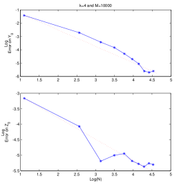
Figure 1: Log-Error curve to estimate $(Y_{0},Z_{0})$, European Call case.

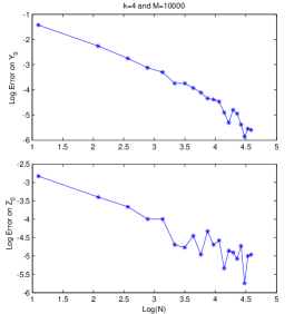
Figure 2: Log-Error curve to estimate $(Y_{0},Z_{0})$, European Put.

On the following graphic, we compare the convergence result of the regression-later algorithm (in blue) with the standard implicit Backward Euler-Maruyama scheme $(S.I)$ of Section 3 in the particular case of a Call option valuation. The implicit Euler scheme $(S.I)$ uses the classical regression-now (cf. [20]) technique to evaluate the couple $(Y_{0},Z_{0})$. It is the customary approach represented in red.

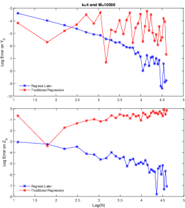
Figure 3: Comparison Log-Error curve (European Call).

The graphics of the above figure shows that the error curves are volatile when we increase the number of time instances. The volatility effect seems to be persistent regarding the approximation of $Z_{0}$ with the scheme $(S.I)$. In other words, the results seem to be more volatile with the standard implicit Backward Euler-Maruyama scheme $(S.I)$ in this particular case choice of $M$ and $k$. As an alternative approach, the regression-later approach shows a stable converge trend and less volatile that the result of the scheme scheme $(S.I)$. The same remarks are applied to the European Put case. This graphical results shows that the regression-later approach: as an alternative approach, could offer several advantages in comparison to the regression-now technique.

Application 2: Brownian Functional Case

In this example, the underlying process is assumed to be a standard Brownian motion $W$ on the time interval $[0,T]$. In other words, the forward process is simply a Brownian motion and the terminal condition is a functional of the Brownian motion $W$. We consider the BSDE

$$\left\{\begin{aligned} -&dY_{t}=f(t,W_{t},Y_{t},Z_{t})dt-Z_{t}dW_{t},\qquad 0\leq t<1,\\ &Y_{1}=\phi(W_{1}),\end{aligned}\right.$$ (5.2)

where the terminal function and the driver function are defined by

$$\left\{\begin{aligned} &\phi(x)=x\arctan(x)-\ln(\sqrt{1+x^{2}})\\ &f(t,W_{t},Y_{t},Z_{t})=-\frac{1}{2(1+\tan^{2}(Z_{t}))}.\end{aligned}\right.$$

It is easy to check by Itô’s formula that, the solution of the above system is almost surely

$$(Y_{t},Z_{t})=(-\frac{1}{2}\ln(1+W_{t}^{2})+W_{t}\arctan(W_{t}),\arctan(W_{t})).$$

By noting that the function $x\mapsto\ln(x)$ satisfies the linear growth condition and the function $x\mapsto\arctan(x)$ is bounded, the unique solution of (5.2) satisfies

$$(Y_{t},Z_{t})_{0\leq t\leq T}\in\mathcal{S}^{2}(\mathbb{R})\times\mathcal{H}^{2}(\mathbb{R}).$$

The exact value of the couple $(Y,Z)$ at the time point $t_{0}$ is $({Y}_{0},{Z}_{0})=(0,0)$. The figure below shows the empirical logarithm of the absolute error induced by the numerical estimation of the couple $({Y}_{0},{Z}_{0})$.

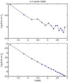
Figure 4: Log-Error curve to estimate $(Y_{0},Z_{0})$

Modulo the choice of $|\pi|$ and the number of the basis function $k$, the graphics show a stable convergence result. This leads us to the same conclusion as above regarding the estimation of the couple $(Y_{0},Z_{0})$. Nevertheless the estimation of the initial value $Y_{0}$ is more stable and quicker than the estimation of the initial value $Z_{0}$ in the first example. The convergence order could be also accelerated by two-step schemes or the Runge-Kutta methods (see e.g. [11], [10], [2]).

6 Conclusion

We have discussed a new numerical scheme for backward stochastic differential equations (BSDEs). The scheme is based on the regression-later approach. In the first part of our work, we introduced the theory of BSDEs, gave some general background on their studies and reviewed the classical backward Euler-Maruyama scheme. In the next step, we described our regression-later algorithm in detail and derived a convergence result of the scheme. Finally, we provided two numerical experiments to illustrate the performance of the regression-later algorithm: the first in the context of option pricing and the second in the case where the terminal condition is a functional of a Brownian motion. Modulo a suitable choice of the number of discretization points and the number of basis functions, our numerical results show a stable convergence regarding the estimation of the solution $(Y,Z)$. In many numerical algorithms for solving BSDEs, one of the difficulties is to solve a dynamic programming problem which involves often the computation of conditional expectations at each step across the time interval. We remark that in many alternative algorithms, the numerical computation of $Z$ is more challenging than the computation of the process $Y$, leading to potential numerical instabilities especially in higher dimensions. It is interesting to note that our algorithm circumvents this difficulty, by obtaining the numerical approximation of the $Z$ process directly from the approximation of $Y$ and the basis functions. Our numerical results look highly promising, but more future researches are needed particularly regarding the global analysis of the error on the estimation of $(Y,Z)$.

7 Appendix

Lemma 7.1.

For any constant $\alpha>0$ and for any $a,b\in\mathbb{R}$,

$$(a+b)^{2}\leq(1+\alpha)a^{2}+(1+\frac{1}{\alpha})b^{2}.$$ (7.1)

Proof.

The result is a direct consequence of Young’s inequality. ∎

Let us now recall the classical discrete Gronwall Lemma (see, e.g. [39] or [33]) .

Lemma 7.2 (Gronwall Inequality A).

Let us consider the partition

$$\pi:0=t_{0}<...<t_{N}=T$$

of the interval $[0,T]$ and let $\Delta_{i}$ be its mesh. We also consider the families $(a_{k})_{0\leq k\leq N},(b_{k})_{0\leq k\leq N},$ assumed to be non-negative such that for some positive constant $\gamma>0$ we have:

$$a_{k-1}\leq(1+\gamma\Delta_{i})a_{k}+b_{k},\quad k=1,\dots,N.$$

Then,

$$\quad\max_{0\leq i\leq N}a_{i}\leq e^{\gamma T}(a_{N}+\sum_{i=1}^{N}b_{i}).$$

Lemma 7.3 (Gronwall Inequality B).

Let $y,b,a:[0,T]\mapsto\mathbb{R}$ be three continuous functions such that, $b$ is non-negative and

$$y(t)\leq a(t)+\int_{0}^{t}b(s)y(s)ds,\qquad 0\leq t\leq T.$$

Then,

$$y(t)\leq a(t)+\int_{0}^{t}a(s)b(s)\exp\bigg{(}\int_{s}^{t}b(u)du\bigg{)}ds,\qquad 0\leq t\leq T.$$

In addition, if the function $a$ is non-decreasing, then

$$y(t)\leq a(t)\exp\bigg{(}\int_{0}^{t}b(s)ds\bigg{)},\qquad 0\leq t\leq T.$$

References

- [1] S. Alanko and M. Avellaneda, Reducing variance in the numerical solution of bsdes, Comptes Rendus Mathematique, 351 (2013), pp. 135–138.
- [2] U. M. Ascher, S. J. Ruuth, and R. J. Spiteri, Implicit-explicit runge-kutta methods for time-dependent partial differential equations, Applied Numerical Mathematics, 25 (1997), pp. 151–167.
- [3] V. Bally, Approximation scheme for solutions of bsde, Pitman research notes in mathematics series, (1997), pp. 177–192.
- [4] G. Barles and E. Lesigne, Sde, bsde and pde, Pitman Research Notes in Mathematics Series, (1997), pp. 47–82.
- [5] C. Bender and J. Steiner, A posteriori estimates for backward sdes, SIAM/ASA Journal on Uncertainty Quantification, 1 (2013), pp. 139–163.
- [6] E. Beutner, A. Pelsser, and J. Schweizer, Fast convergence of regress-later estimates in least squares monte carlo, Available at SSRN 2328709, (2013).
- [7] J. Bismut, Conjugate convex functions in optimal stochastic control, Journal of Mathematical Analysis and Applications, 44 (1973), pp. 384–404.
- [8] B. Bouchard and N. Touzi, Discrete-time approximation and monte-carlo simulation of backward stochastic differential equations, Stochastic Processes and their Applications, 111 (2004), pp. 175–206.
- [9] P. Briand and C. Labart, Simulation of bsdes by wiener chaos expansion, The Annals of Applied Probability, 24 (2014), pp. 1129–1171.
- [10] J. Butcher, Runge-kutta methods for ordinary differential equations, in COE Workshop on Numerical Analysis Kyushu University, 2005.
- [11] J.-F. Chassagneux and D. Crisan, Runge–kutta schemes for backward stochastic differential equations, The Annals of Applied Probability, 24 (2014), pp. 679–720.
- [12] J.-F. Chassagneux and A. Richou, Numerical simulation of quadratic bsdes, The Annals of Applied Probability, 26 (2016), pp. 262–304.
- [13] P. Cheridito, H. M. Soner, N. Touzi, and N. Victoir, Second-order backward stochastic differential equations and fully nonlinear parabolic pdes, Communications on Pure and Applied Mathematics, 60 (2007), pp. 1081–1110.
- [14] D. Chevance, Résolution numérique des équations différentielles stochastiques rétrogrades, PhD thesis, Universtité de Provence, 1997.
- [15] D. Crisan and K. Manolarakis, Solving backward stochastic differential equations using the cubature method: application to nonlinear pricing, SIAM Journal on Financial Mathematics, 3 (2012), pp. 534–571.
- [16] L. Delong, Backward stochastic differential equations with jumps and their actuarial and financial applications, Springer, 2013.
- [17] D. Duffie and L. G. Epstein, Stochastic differential utility, Econometrica: Journal of the Econometric Society, (1992), pp. 353–394.
- [18] N. El Karoui, S. Hamadène, and A. Matoussi, Backward stochastic differential equations and applications, Indifference pricing: theory and applications, (2008), pp. 267–320.
- [19] N. El Karoui, S. Peng, and M. C. Quenez, Backward stochastic differential equations in finance, Mathematical finance, 7 (1997), pp. 1–71.
- [20] P. Glasserman and B. Yu, Simulation for american options: regression now or regression later?, in Monte Carlo and Quasi-Monte Carlo Methods 2002, Springer, 2004, pp. 213–226.
- [21] E. Gobet and C. Labart, Error expansion for the discretization of backward stochastic differential equations, Stochastic processes and their applications, 117 (2007), pp. 803–829.
- [22] E. Gobet, J. Lemor, and X. Warin, A regression-based Monte Carlo method to solve backward stochastic differential equations, Annals of Applied Probability, 15 (2005), pp. 2172–2202.
- [23] E. Gobet and P. Turkedjiev, Approximation of backward stochastic differential equations using malliavin weights and least-squares regression, Bernoulli, 22 (2016), pp. 530–562.
- [24] B. Gong and H. Rui, One order numerical scheme for forward–backward stochastic differential equations, Applied Mathematics and Computation, 271 (2015), pp. 220–231.
- [25] S. Hamadène and M. Jeanblanc, On the starting and stopping problem: application in reversible investments, Mathematics of Operations Research, 32 (2007), pp. 182–192.
- [26] Y. Hu, P. Imkeller, and M. Müller, Utility maximization in incomplete markets, The Annals of Applied Probability, 15 (2005), pp. 1691–1712.
- [27] T. P. Huijskens, M. Ruijter, and C. W. Oosterlee, Efficient numerical fourier methods for coupled forward–backward sdes, Journal of Computational and Applied Mathematics, 296 (2016), pp. 593–612.
- [28] C. B. Hyndman and P. O. Ngou, Global convergence and stability of a convolution method for numerical solution of bsdes, arXiv preprint arXiv:1410.8595, (2014).
- [29] N. Ikeda and S. Watanabe, Stochastic differential equations and diffusion processes, Elsevier, 2014.
- [30] A. Khedher and M. Vanmaele, Discretisation of fbsdes driven by càdlàg martingales, Journal of Mathematical Analysis and Applications, 435 (2016), pp. 508–531.
- [31] R. J. Laeven and M. Stadje, Robust portfolio choice and indifference valuation, Mathematics of Operations Research, 39 (2014), pp. 1109–1141.
- [32] J. Ma, P. Protter, and J. Yong, Solving forward-backward stochastic differential equations explicitly a four step scheme, Probability Theory and Related Fields, 98 (1994), pp. 339–359.
- [33] J. Mémin, S. Peng, and M. Xu, Convergence of solutions of discrete reflected backward sde’s and simulations, Acta Mathematicae Applicatae Sinica, English Series, 24 (2008), pp. 1–18.
- [34] D. Nualart, The Malliavin calculus and related topics, vol. 1995, Springer, 2006.
- [35] E. Pardoux and S. Peng, Adapted solution of a backward stochastic differential equation, Systems & Control Letters, 14 (1990), pp. 55–61.
- [36] , Backward stochastic differential equations and quasilinear parabolic partial differential equations, in Stochastic partial differential equations and their applications, Springer, 1992, pp. 200–217.
- [37] L. Stentoft, Convergence of the least squares monte carlo approach to american option valuation, Management Science, 50 (2004), pp. 1193–1203.
- [38] W. A. Ventura and A. Korzeniowski, On discretely reflected backward stochastic differential equations, Stochastic Analysis and Applications, 34 (2016), pp. 1–23.
- [39] J. Zhang, A numerical scheme for bsdes, Annals of Applied Probability, 14 (2004), pp. 459–488.
- [40] W. Zhao, L. Chen, and S. Peng, A new kind of accurate numerical method for backward stochastic differential equations, SIAM Journal on Scientific Computing, 28 (2006), pp. 1563–1581.