Activity cycles in members of young loose stellar associations

Abstract

Context. Magnetic cycles analogous to the solar one have been detected in tens of solar-like stars by analyzing long-term time-series of different magnetic activity indexes. The relationship between the cycle properties and global stellar parameters is not fully understood yet. One reason for this is the sparseness of the data.

Aims. In the present paper we searched for activity cycles in a sample of 90 young solar-like stars with ages between 4 and 95 Myr with the aim to investigate the properties of activity cycles in this age range.

Methods. We measured the length $P_{\rm cyc}$ of a given cycle by analyzing the long-term time-series of three different activity indexes: the period of rotational modulation, the amplitude of the rotational modulation and the median magnitude in the V band. For each star, we computed also the global magnetic activity index ¡IQR¿ that is proportional to the amplitude of the rotational modulation and can be regarded as a proxy of the mean level of the surface magnetic activity.

Results. We detected activity cycles in 67 stars. Secondary cycles were also detected in 32 stars of the sample. The lack of correlation between $P_{\rm cyc}$ and $P_{\rm rot}$ and the position of our targets in the $P_{\rm cyc}/P_{\rm rot}-Ro^{-1}$ diagram suggest that these stars belong to the so-called Transitional Branch and that the dynamo acting in these stars is different from the solar one and from that acting in the older Mt. Wilson stars. This statement is also supported by the analysis of the butterfly diagrams whose patterns are very different from those seen in the solar case. We computed the Spearman correlation coefficient $r_{\rm S}$ between $P_{\rm cyc}$, ¡IQR¿ and different stellar parameters. We found that $P_{\rm cyc}$ in our sample is uncorrelated with all the investigated parameters. The ¡IQR¿ index is positively correlated with the convective turn-over time-scale, the magnetic diffusivity time-scale $\tau_{\rm diff}$, and the dynamo number $D_{\rm N}$, whereas it is anti-correlated with the effective temperature $T_{\rm eff}$, the photometric shear $\Delta\Omega_{\rm phot}$ and the radius $R_{\rm C}$ at which the convective zone is located. We investigated how $P_{\rm cyc}$ and ¡IQR¿ evolve with the stellar age. We found that $P_{\rm cyc}$ is about constant and that ¡IQR¿ decreases with the stellare age in the range 4-95 Myr. Finally we investigated the magnetic activity of the star AB Dor A by merging ASAS time-series with previous long-term photometric data. We estimated the length of the AB Dor A primary cycle as $P_{\rm cyc}=16.78\pm 2\rm yr$ and we found also shorter secondary cycles with lengths of 400 d, 190 d and 90 d respectively.

1 Introduction

The present paper addresses the occurrence and properties of magnetic activity cycles in young solar-like stars with ages spanning the range $4-95\leavevmode\nobreak\ \rm Myr$. The study of activity cycles requires the availability of long-term time-series of one or more magnetic activity indexes.

The Solar magnetic activity has been well monitored in time by recording the measurements of different activity indexes such as the Total Solar Irradiance (TSI), the sunspots number, the flare occurrence rate, and the intensity of specific spectral lines. The analysis of long-term time-series of these activity proxies revealed that the Sun exhibits periodic or quasi-periodic variability phenomena occurring over different time-scales ranging from 30 d to 80 yr. The 30-d periodicity is induced by the solar rotation that modulates the visibility of spots and faculae over the solar disk. A 11-yr period, the so-called Schwabe cycle, is related to the evolution of the solar magnetic field and is associated with a cyclic variation of the sunspots number and of the average latitude at which spots and faculae occur.

The level of the solar magnetic activity is a complex function of time and other signals are superimposed over the 11-yr cycle.

A 154-d periodicity, for instance, was detected in $\gamma$-ray activity (Rieger et al. 1984), in the Mt. Wilson sunspot index (Ballester et al. 2002), and in the sunspot area (Lean 1990; Oliver et al. 1998). These 154-d cycles are usually named ”Rieger cycles” because they were detected, for the first time, by Rieger et al. (1984).

The expression ”quasi-biennial variations” is instead used to refer to periodic or quasi-periodic phenomena that occur with time-scales ranging from 1 yr to 3 yr. Gnevyshev (1967, 1977), for instance, analyzed variations in sunspots numbers, large flares occurrence rate and coronal green-line emission and found that each solar cycle exhibits two maxima separated by 2-3 yr intervals. Variability phenomena occurring in a 2-yr time-scale have also been detected in the 35-years TSI time-series analyzed by Ferreira Lopes et al. (2015). A review of the quasi-biennial variations detected in solar activity and of the physical processes invoked to explain such variations can be found in Hathaway (2015). Finally, on longer time-scales, the Sun activity is characterized by the 22-yr Hale cycle (Hale et al. 1919) associated with a reverse in the sunspots polarity and the 80-yr Gleisseberg cycle (Gleissberg 1958) that is a a cyclic modulation of the amplitude of the 11-yr cycles.

Stars with a spectral type later than F5 have a magnetic activity similar to that observed in the Sun and are therefore characterized by activity cycles similar to those occurring in our star. The analysis of long-term photometric time-series allowed the detection of activity cycles in a wide sample of late-type stars. The first studies on stellar activity cycles were based on the results of the Mount Wilson Ca II H&K survey (Wilson 1968) and were conducted by Wilson (1978), Durney et al. (1981), Baliunas & Vaughan (1985) and Baliunas et al. (1995). These authors measured the rotation period $P_{\rm rot}$ and the cycle length $P_{\rm cyc}$ for tens of stars by analyzing the temporal variations of the photometric fluxes in two 0.1 nm passbands centered on the core of the Ca II H and K emission lines. Recently, Oláh et al. (2016) analyzed the full Ca II H&K time-series collected at Mount Wilson for a sample of 29 stars. Their work exploits 36-year time-series that are ten-years longer than those analyzed by Baliunas et al. (1995) and allow a better frequency resolution.

Messina & Guinan (2002) exploited long-term photometry in the Johnson V band to measure the rotation period $P_{\rm rot}$ and the length of activity cycle $P_{\rm cyc}$ in a sample of six young solar analogues. Oláh et al. (2009) analyzed long-term spectroscopic and photometric observations to study the activity cycles in a sample of 20 late type-stars.

Lehtinen et al. (2016) studied activity trends in a sample of 21 young solar-type stars by analyzing long-term photometry collected in Johnson B and V bands. Suárez Mascareño et al. (2016) detected long-term activity cycles in a sample of 49 nearby main-sequence stars by analyzing the V-band time-series collected by the ASAS survey (All Sky Automatic Survey, Pojmanski 1997). Recently, high precision photometric time-series acquired by space-borne telescopes were used to study stellar cycles. Vida et al. (2014), for instance, exploited Kepler data to study activity cycles in 39 fast-rotating late-type stars and Ferreira Lopes et al. (2015) studied activity cycles in 16 late-type stars by analyzing CoRoT time-series.

Since stellar activity cycles have been detected, a link has been searched between the cycle length $P_{\rm cyc}$, the magnetic activity indexes and global stellar parameters like the rotation period $P_{\rm rot}$, the Rossby Number $Ro$ and the age (see e.g. See et al. 2016; Oláh et al. 2016; García et al. 2014, and references therein). These relationships are important to probe the theoretical models developed to simulate the magnetic dynamos. The data currently available are still incomplete especially for young solar-like stars and the picture of the relationships between magnetic activity and global stellar parameters is far from being clear.

The relationship between the parameters $P_{\rm cyc}$ and $P_{\rm rot}$ is, for instance, not fully understood. Several authors found that $P_{\rm cyc}$ and $P_{\rm rot}$ are correlated with each other (see e.g. Baliunas et al. 1996; Böhm-Vitense 2007; Oláh et al. 2009, 2016). Other authors found no correlation between the two parameters (Lehtinen et al. 2016). Other works found a correlation in main-sequence F, G and K stars and no correlation in M type stars (Savanov 2012; Vida et al. 2014; Suárez Mascareño et al. 2016). This last feature has been interpreted as a difference in the dynamo mechanisms acting in FGK stars and M stars.

The study of the relationship between the $\frac{P_{\rm cyc}}{P_{\rm rot}}$ ratio and the Rossby number showed that stars seem to lie in different activity branches (see e.g. Brandenburg et al. 1998; Lehtinen et al. 2016) possibly connected to different kinds of dynamos. Böhm-Vitense (2007) remarked that the Sun has an anomalous position with respect to these branches. It is unclear if the Sun is a special case or if other stars exhibit a similar behavior.

The evolution of the $\frac{P_{\rm cyc}}{P_{\rm rot}}$ ratio with the stellar age has been studied by Soon et al. (1993) and, more recently, by Oláh et al. (2016) in the age range 200-6200 Myr.

In the present work we searched for activity cycles in a sample of 90 late-type stars belonging to young loose stellar associations. In Distefano et al. (2016) (hereafter Paper I) we investigated the rotational properties of these stars and we determined a lower limit for their SDR (Surface Differential Rotation). In the present paper we focused in their magnetic activity. As, remarked in Paper I, the ages and the spectral types of these stars span the ranges 4-95 Myrs and G5-M4, respectively. This means that our sample comprises both fully convective stars as well as stars with a radiative core surrounded by a convective envelope. Hence the data used here allow the characterization of activity cycles in stars with different structures and ages and to extend the age range investigated by Soon et al. (1993) and Oláh et al. (2016).

The data used to perform our analysis and the procedure followed to measure the length of activity cycles are described in Sec. 2 and in Sec. 3, respectively. The results of our analysis are reported in Sec. 4 and discussed in Sec. 5. In Sec. 6, the conclusions are drawn.

2 Data

2.1 Targets

In this paper we exploited long-term photometric time-series collected by the ASAS survey (All Sky Automatic Survey, Pojmanski 1997) and we searched for activity cycles in a sample of 90 solar-like stars belonging to young loose stellar associations. These targets are listed in Table 3.1 together with their main astrophysical parameters. In Table 1 we reported, for each association, the number of stars investigated and the number of stars in which we were able to detect one or more activity cycles. The same ASAS time-series have been exploited in Paper I to investigate the rotational properties of our target stars.

Note that in Paper I we also investigated 22 stars for which the Super-WASP (Butters et al. 2010) time-series were available. These data have a photometric accuracy better than ASAS data. However, a typical Super-WASP datasets spans only a 4-year interval and is characterized by observation gaps of several months. The ASAS time-series, despite their lower photometric precision, are best suited to study long-term variability. Indeed these time-series span an interval of about 9 years and are characterized by shorter observation gaps due to the use of two different observing stations located at Las Campanas Observatory, Chile and at Haleakala, Maui, Hawaii, respectively. For this reason we decided to analyze the ASAS data only.

2.2 Magnetic activity indexes

All works cited in the introduction measured the lengths of activity cycles by searching for a periodicity in long-term time-series of different activity indexes.

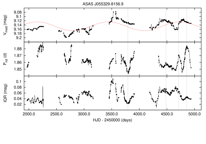
Figure 13: Top panel: the $V_{\rm med}$ time-series for the star ASAS J055329-8156.9. Mid panel; the $P_{\rm rot}$ time-series. Bottom panel: the IQR time-series. A primary cycle with length $P_{\rm cyc}=1290\leavevmode\nobreak\ d$ was detected in the $V_{\rm med}$ time-series and the sinusoid best-fitting the data was over-plotted on it (red dashed line). The $P_{\rm rot}$ and the IQR time-series exhibit cycles (dark continuous lines) shorter than the primary one. The black dotted lines mark the times at which maxima and minima occur in the $P_{\rm rot}$ time-series.

In the present paper, we exploited the long-term time-series of three activity indexes that have been obtained from the analysis of the photometric data collected by the ASAS survey. In Paper I, we processed the ASAS data with a sliding window algorithm that divided each photometric time-series in segments of a given length T. For each segment, we computed three activity indexes: the rotation period $P_{\rm rot}$, inferred by the rotational modulation of the light curve by magnetically Active Regions (ARs), the median magnitude ($V_{\rm med}$), and the Inter-Quartile Range (IQR) defined as the difference between the 75-th and the 25-th percentiles of V magnitude values (different examples of these activity indexes time-series can be seen in Figs. 2-5 of Paper I and in Figs. 1-4, 12-13 of the present work.)

In Paper I we processed the ASAS photometric time-series by using three different values of the sliding-window length, i.e. T=50 d, 100 d and 150 d, producing three different time-series for each activity index. The results given in Paper I have been inferred by the time-series obtained with T=50 d. As discussed there, the use of sliding-window lengths of T =100 d and T = 150 d tends to filter out the variability phenomena occurring over a time-scale shorter than 100 d, flattening the amplitude variations of the different activity indexes (see. Figs. 2-5 of Paper I). However, the activity indexes time-series obtained with T=100 and 150 d are more regular and smoother than those obtained with T=50 d and are more suitable to detect long-term variations due to activity cycles. Therefore, while T=50 d is an optimal choice for analyzing SDR as in Paper I, longer segments, e.g. T=100 d as used here, are better suited to search for activity cycles. This difference in T obviously does not introduce any inconsistencies in, e.g., correlation analysis between activity cycles and SDR.

In Paper I, we showed that the rotation period detected in different segments slightly changes in time. This trend could be induced by the combined effect of stellar Surface Differential Rotation (SDR) and of ARs migration in latitude. Indeed ARs placed at different latitudes rotate with different frequencies in case of SDR. The ARs migration, due to a Schwabe-like cycle, induces a temporal variation in the detected photometric period $P_{\rm rot}$. Such a parameter can be therefore regarded as a tracer of the spot latitude migration.

Note that this activity index has to be treated with caution. Lehtinen et al. (2016) and Lanza et al. (2016) noticed that the different rotation periods detected in different segments could be also a consequence of the ARs growth and decay occurring simultaneously at various latitudes and longitudes on the star. However, as remarked by Lehtinen et al. (2016), the use of segments with a short duration should limit this effect (see the discussion on the sliding-window length in Sec. 3.1 of Paper I and in Sec. 4.1 of Lehtinen et al. (2016) for more details). This activity index has been recently used by Vida et al. (2014) to investigate stellar cycles on Kepler data.

The $V_{med}$ index is related to the axisymmetric part of the spot distribution on the stellar surface. In fact, the higher the fractional area covered by spots evenly distributed in longitude, the lower the average photometric flux in the V band,. This is one of the most used activity index to investigate activity cycles (see e.g. Rodonò et al. 2000; Messina & Guinan 2002; Lehtinen et al. 2016)

The IQR index is proportional to the stellar variability amplitude. The variability amplitude is also an index widely used to study activity cycles (see e.g. Rodonò et al. 2000; Ferreira Lopes et al. 2015; Lehtinen et al. 2016). Note that the variability of solar-like stars is due to different phenomena acting in different time-scales like the intrinsic evolution of spots and faculae, the intrinsic evolution of ARs complexes and the flux rotational modulation induced by ARs. In this paper, the IQR index was computed in 100-d long segments. In these intervals the main source of variability is the rotational modulation (see e.g. Messina & Guinan 2002; Lanza et al. 2003). Hence the IQR index is proportional to the amplitude of the rotational modulation signal and is related to the non-axisymmetric part of the spot distribution.

Finally, for each star we computed also a global magnetic index that is given by the average value ¡IQR¿ of the IQR time-series. The ¡IQR¿ values are reported in Table 3.1 for all the stars investigated here.

Table 1: Stellar associations investigated in the present work.

Association	age	$N_{stars}$	$N_{cyc}$
	Myr
$\epsilon$ Chamaleontis ($\epsilon$ Cha)	3-5	9	6
$\eta$ Chamaleontis ($\eta$ Cha)	6-10	4	4
TW Hydrae (TWA)	8-12	6	4
$\beta$ Pictoris ($\beta$ Pic)	12-22	13	11
Octans (Oct)	20-40	1	1
Columba (Col)	20-40	6	4
$\eta$ Carinae ($\eta$ Car)	20-40	12	7
Tucana-Horologium (Tuc/Hor)	20-40	16	13
Argus (Arg)	30-50	10	10
IC 2391	30-50	3	3
AB Doradus (AB Dor)	70-120	10	6

2.3 Computation of the global parameters for the target stars

In this paper we investigate the relationships between the cycles lengths $P_{\rm cyc}$, the activity index ¡IQR¿, and the global parameters of our targets. Our analysis was focused on the following parameters: the photometric shear $\Delta\Omega_{\rm phot}$, the effective temperature $T_{\rm eff}$, the convective turnover time-scale $\tau_{\rm C}$, the Rossby number $Ro$, the radius at the bottom of the convection zone $R_{\rm C}$, the dynamo number $D_{\rm N}$, and the magnetic diffusivity time-scale $\tau_{\rm diff}$. $\Delta\Omega_{\rm phot}$, $T_{\rm eff}$, $\tau_{C}$ and $Ro$ have been computed in Paper I where as $R_{\rm C}$, $D_{\rm N}$ and $\tau_{\rm diff}$ have been computed in this work for the first time.

The photometric shear of a given star is defined as

$$\Delta\Omega_{\rm phot}=\Omega_{\rm max}-\Omega_{\rm min}=\frac{2\pi}{P_{\rm min}}-\frac{2\pi}{P_{\rm max}}$$ (1)

where $P_{\rm min}$ and $P_{\rm max}$ are the minimum and maximum values of the $P_{\rm rot}$ index and are interpreted as the rotation periods of two Active Regions occurring at two different latitudes. This parameter can be regarded as a lower limit for the SDR that is defined as

$$\Delta\Omega=\Omega_{\rm Eq}-\Omega_{\rm pole}$$ (2)

where $\Omega_{\rm Eq}$ and $\Omega_{\rm pole}$ are the stellar rotation frequencies at the equator and at the poles.

The effective temperature $T_{\rm eff}$ and the convective turnover time-scale $\tau_{\rm C}$ have been derived in Paper I using Spada et al. (2013).

The Rossby number $Ro$ is defined as:

$$Ro\equiv\frac{P_{\rm rot}}{\tau_{\rm C}},$$ (3)

where $\tau_{\rm C}$ is derived by the theoretical isochrones of Spada et al. (2013). Other works (Saar & Brandenburg 1999; Lehtinen et al. 2016) use the definition given by Brandenburg et al. (1998):

$$Ro\equiv\frac{P_{\rm rot}}{4\pi\tau_{\rm C}}.$$ (4)

In these works, the convective turnover time-scale is computed through the semi-empirical equation given by Noyes et al. (1984) that expresses $\tau_{\rm C}$ as a function of the color index $B-V$. In order to make a comparison between our results and those of the above mentioned works, we computed the Ro values according to the Eq. (4) and by using the $\tau_{\rm C}$ values as given by the formula of Noyes et al. (1984). In the rest of the paper, the values computed by means of Eq. 4 will be indicated with the symbol $Ro_{\rm Br}$ where $\rm Br$ stands for Brandenburg.

The dynamo number is defined as:

$$D_{\rm N}=\frac{\alpha\Delta\Omega D_{\rm CZ}^{3}}{\eta_{t}^{2}},$$ (5)

with

$$\alpha=\frac{l_{\rm m}^{2}}{H_{D}}\Omega,$$ (6)

where $D_{\rm CZ}$ is the depth of the convective zone, $l_{\rm m}$ is the mixing-length and $H_{D}$ is the density scale-height, $\eta_{t}$ is the turbulent diffusivity and $\Delta\Omega$ the rotational shear. The parameters $D_{\rm CZ}$, $\eta_{t}$, $l_{\rm m}$ and $H_{D}$ occurring in Eq. 5 and 6 were derived by the theoretical models of Spada et al. (2013). The parameter $\Delta\Omega$ was replaced with the parameter $\Delta\Omega_{\rm phot}$ computed in Paper I.

Finally, the magnetic diffusivity time-scale is defined as:

$$\tau_{\rm diff}=\frac{D_{\rm CZ}^{2}}{\eta_{t}}$$ (7)

where $\eta_{t}$ is the turbulent diffusivity; $\tau_{\rm diff}$ is the time-scale for the turbulent dissipation of magnetic energy over a length scale $D_{\rm CZ}$. All the parameters computed for the different targets are reported in Table 3.1.

3 The method

We searched for activity cycles by running the Lomb-Scargle (Lomb 1976; Scargle 1982) and the PDM (Phase Dispersion Minimization; Jurkevich 1971; Stellingwerf 1978) algorithms on the $P_{\rm rot}$, the $V_{\rm med}$ and the IQR time-series. The ASAS time-series span, on average, an interval T=3000 days. We assumed, as in Distefano et al. (2012), that a period P can be detected if $P\leq 0.75T$ and we performed our period search in the range (100-2000 d). We computed the FAP (False Alarm Probability) associated with a given period $P_{\rm cyc}$ according to the procedure described in Sec. 3.1 and we flagged a period as valid if it satisfied the requirement $\rm FAP<0.1\%$. In some time-series, visual inspection allowed the identification of cyclical patterns that the Lomb-Scargle and the PDM algorithm were not able to detect. The failure of the period search algorithms is due to the “quasi-periodic” nature of the stellar cycles and can be ascribed to different reasons: in some cases a cyclical pattern occurs only in a limited interval of the whole time-series; in other cases a cyclical pattern is visible in the complete time-series, but the length of the cycle changes in time. Finally, in some cases, the visual inspection suggests that the star is characterized by a cycle longer than the whole time-series length. Since the size of our sample is relatively small, we decided to visually inspect each time-series aiming at detecting and measuring the lengths of the cycles missed by the Lomb-Scargle and the PDM algorithms. In this case, we flagged a $P_{\rm cyc}$ value as valid if at least one complete oscillation is visible (i.e. if at least two consecutive maxima or minima are clearly visible).

The uncertainty on $P_{\rm cyc}$ is estimated through the equation:

$$\delta P_{\rm cyc}=\frac{\delta\nu_{\rm cyc}}{\nu_{\rm cyc}^{2}}$$ (8)

where $\delta\nu_{\rm cyc}$ is the uncertainty associated with the frequency of the cycle $\nu_{\rm cyc}=1/P_{\rm cyc}$. This uncertainty is given by the equation:

$$\delta\nu_{\rm cyc}=\sqrt{{\delta\nu}_{\rm samp}^{2}+\delta\nu_{\rm noise}^{2}}$$ (9)

where $\delta\nu_{\rm samp}$ is the uncertainty due to the limited and discrete sampling of time-series and $\delta\nu_{\rm noise}$ is the uncertainty due to data noise; $\delta\nu_{\rm samp}$ and $\delta\nu_{\rm noise}$ are computed according to Kovacs (1981) through the equations

$$\delta\nu_{\rm samp}=\frac{0.16}{\sqrt{2}\nu_{\rm cyc}T^{2}}.$$ (10)

$$\delta\nu_{\rm noise}=\frac{3\sigma}{4\sqrt{N}\nu_{\rm cyc}TA}$$ (11)

where T is the interval time spanned by the time-series, $\sigma$ is the standard deviation of the data before subtracting any periodic signal, $N$ the number of time-series points, and $A$ the amplitude of the signal. In cases in which $P_{\rm cyc}$ values were determined by visual inspection we did not give a $\delta P_{\rm cyc}$ estimate since there is not an objective way to obtain it.

3.1 FAP computation

The typical Monte Carlo method used to assess the FAP of a given period $P_{0}$, that has a power $z_{0}$ in the Lomb-Scargle periodogram, consists in simulating N synthetic time-series with the same sampling of the original time-series. The synthetic data-points are usually generated by means of the equation:

$$x_{i}=<x>+R(0,\sigma)$$ (12)

where $<x>$ is the mean value of the original time-series and $R(0,\sigma)$ is a gaussian random variate with a zero mean and a dispersion $\sigma$ given by the standard deviation associated with the real data-points. The Lomb-Scargle periodogram is computed for each time-series and the highest peak $Z_{\rm max}$ is retained for each periodogram. The FAP associated with $P_{0}$ is then computed as the fraction of synthetic time-series for which $Z_{\rm max}\leavevmode\nobreak\ \geq z_{0}$.

The previous approach is valid only if the points of the original time-series are uncorrelated i.e. if two consecutive data points are independent of each other (see for example the discussion in Herbst & Wittenmyer 1996; Stassun et al. 1999; Rebull 2001). This is not the case of our time-series where two consecutive elements of the activity indexes have been computed in segments that partially overlap with each other.

For this reason, we estimated the FAP by means of the Monte Carlo approach suggested by Brown et al. (1996) and also adopted by Rebull (2001) and Parihar et al. (2009). In this approach, the synthetic data-points are generated by means of a recursive procedure:

$$\begin{array}[]{l}\displaystyle x_{0}=R(0,\sigma)\\ \displaystyle x_{i>0}=\alpha x_{i-1}+\beta R(0,\sigma)\end{array}$$ (13)

where $x_{0}$ and $x_{i}$ are the first element and the i-th element of the simulated time-series and $R(0,\sigma)$ denotes a Gaussian random variate centered on zero with dispersion $\sigma$ (equal to the standard deviation of the real data). The parameters $\alpha$ and $\beta$ are defined as

$$\begin{array}[]{l}\alpha=exp(-\Delta t/L_{corr})\\ \beta=(1-\alpha^{2})^{1/2}\end{array}$$ (14)

where $\Delta t=t_{i}-t_{i-1}$ is the time interval between the two consecutive points $x_{i-1}$ and $x_{i}$, and $L_{corr}$ is the correlation time-scale. The time-series defined by Eqs. (13) is such that two points $x_{i}$ and $x_{j}$ satisfy the property

$$C_{2}(i,j)=exp(-\Delta t_{ij}/L_{corr})$$ (15)

where $C_{2}(i,j)$ is the two-points correlation function and $\Delta t_{ij}=t_{i}-t_{j}$ the time between $x_{i}$ and $x_{j}$ (Brown et al. 1996). In our case, we adopted $L_{corr}=T/3$ were T is the length of the sliding window used to generate the activity index time-series.

In order to assess the FAP probability associated with the period detected in a given time-series we followed the Monte Carlo procedure described above by generating 10000 synthetic time-series. If the period was found by means of the Lomb-Scargle algorithm, the FAP was computed by taking the fraction of synthetic time-series for which $Z_{\rm max}>z_{0}$. If the period $P_{0}$ was found by means of the PDM algorithm, we run the PDM on each synthetic time-series and we retained the minimum value $\theta_{\rm min}$ of the PDM periodogram for each time-series. The FAP was then computed by taking the fraction of the synthetic time-series for which $\theta_{0}<\theta_{\rm min}$, where $\theta_{0}$ is the PDM estimator associated with $P_{0}$ .

Figure 1: The $V_{\rm med}$ time-series for the star ASAS J011315-6411.6. A cycle with length $P_{\rm cyc}\leavevmode\nobreak\ =\leavevmode\nobreak\ 1801\leavevmode\nobreak\ d$ was detected by the period-search algorithms. The black line is the sinusoid best-fitting the data.

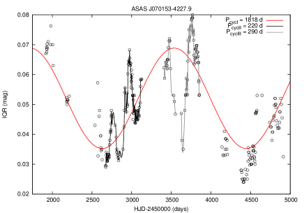
Figure 2: The IQR time-series for the star ASAS J070153-4227.9. A cycle with length $P_{\rm cyc}\leavevmode\nobreak\ =\leavevmode\nobreak\ 1818\leavevmode\nobreak\ d$ (red line) was detected by the period search algorithms. A visual inspection reveals also two shorter cycles with lengths 220 and 290 d, respectively. The dark and gray lines were obtained by fitting the data with smoothing cubic splines and were plotted to highlight the cycles detected by eye.

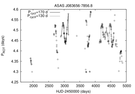
Figure 3: The $P_{\rm rot}$ time-series for the star ASAS J083656-7856.8. A visual inspection revealed two cycles with lengths 170 d and 130 d, respectively. Two smoothing cubic splines are over-plotted to highlight the cycles with the dark and the gray line, respectively.

Figure 4: The $V_{\rm med}$ time-series for the star ASAS J082406-6334.1. The time-series shows a long-term trend suggesting a cycle longer than 3000 d. A short cycle of 180 d is also visibile and highlighted with a smoothing cubic spline in black.

longtablellllllllllllll List of the targets investigated in the present work.
Target ID Assoc. $P_{\rm rot}$ $\Delta\Omega_{\rm phot}$ m $T_{\rm eff}$ $R_{\rm C}$ $\tau_{\rm C}$ $\tau_{\rm diff}$ $D_{\rm N}$Ro $Ro_{\rm Br}$ ¡IQR¿
(d) ($\rm rad\leavevmode\nobreak\ d^{-1}$) $M_{\odot}$ K d d
continued.
Target ID Assoc. $P_{\rm rot}$ $\Delta\Omega_{\rm phot}$ m $T_{\rm eff}$ $R_{\rm C}$ $\tau_{\rm C}$ $\tau_{\rm diff}$ $D_{\rm N}$ Ro $Ro_{\rm Br}$ ¡IQR¿
(d) ($\rm rad\leavevmode\nobreak\ d^{-1}$) $M_{\odot}$ K d d
J001353-7441.3 TUC/HOR 3.67 0.146 0.95 5060.67 0.68 50 544 45182 0.074 0.017 0.038
J002409-6211.1 TUC/HOR 1.75 0.068 0.78 4325.44 0.6 146 1337 192079 0.012 0.005 0.052
J003451-6155.0 TUC/HOR 0.38 0.057 1.03 5446.5 0.74 32 391 98487 0.012 0.001 0.051
J004220-7747.7 TUC/HOR 2.57 0.048 0.86 4608.72 0.63 93 1013 58816 0.028 0.009 0.048
J011315-6411.6 TUC/HOR 1.26 0.045 0.83 4513.54 0.62 119 1075 124198 0.011 0.005 0.078
J015749-2154.1 TUC/HOR 3.05 0.086 1.06 5596.57 0.75 24 163 4490 0.124 0.02 0.035
J020136-1610.0 COL 3.21 0.076 1.07 5649.15 0.75 24 212 5738 0.131 0.011 0.055
J020718-5311.9 TUC/HOR 2.33 0.233 1.04 5499.37 0.74 32 255 32746 0.073 0.015 0.031
J024126+0559.3 BPIC 4.83 0.035 0.83 4115.02 0.55 196 2036 79357 0.025 0.016 0.093
J024233-5739.6 TUC/HOR 7.4 0.071 0.77 4263.07 0.6 146 1348 48069 0.051 0.024 0.056
J030942-0934.8 ABDOR 5.47 0.068 0.95 5545.63 0.72 39 249 3822 0.14 0.022 0.028
J031909-3507.0 TUC/HOR 8.52 0.061 0.71 4000.66 0.57 172 1701 51611 0.05 0.027 0.065
J033049-4555.9 TUC/HOR 3.8 0.122 0.89 4764.23 0.65 93 833 73155 0.041 0.013 0.036
J033156-4359.2 TUC/HOR 2.93 0.07 0.74 4151.49 0.58 172 1476 138328 0.017 0.009 0.057
J034723-0158.3 ABDOR 3.86 0.057 - - - - - - - 0.011 0.070
J045249-1955.0 TUC/HOR 5.21 0.06 1.08 5709.79 0.76 24 189 2332 0.213 0.019 0.062
J045305-4844.6 COL 4.59 0.059 0.9 4820.09 0.65 71 755 24951 0.065 0.017 0.048
J045935+0147.0 BPIC 4.42 0.047 0.8 4015.72 0.53 196 2339 144854 0.023 0.013 0.064
J050047-5715.4 BPIC 8.74 0.05 0.8 4005.8 0.53 196 2365 79212 0.045 0.027 0.049
J050230-3959.2 ABDOR 6.58 0.073 0.68 4320.15 0.68 75 752 18279 0.088 0.024 0.074
J050651-7221.2 Octans 0.24 0.101 - - - - - - - - 0.044
J052845-6526.9 ABDOR 0.51 0.053 0.93 5455.8 0.71 45 294 41297 0.011 0.002 0.068
J052857-3328.3 ABDOR 0.69 0.07 0.88 5274.9 0.7 50 365 56018 0.014 0.002 0.045
J053705-3932.4 TUC/HOR 2.46 0.182 0.95 5038.04 0.68 50 597 97627 0.05 0.01 0.037
J055101-5238.2 COL 1.2 0.081 1.02 5392.94 0.73 32 343 35666 0.038 0.006 0.047
J055329-8156.9 CAR 1.86 0.125 1.09 5760.17 0.76 24 87 4062 0.076 0.008 0.050
J055751-3804.1 ABDOR 0.79 0.143 1.04 5862.33 0.74 32 153 26084 0.024 0.004 0.041
J060834-3402.9 ABDOR 3.4 0.1 - - - - - - - 0.014 0.052
J061828-7202.7 BPIC 2.67 0.045 0.88 4302.06 0.57 173 1504 113230 0.015 0.009 0.052
J062607-4102.9 COL 4.18 0.106 1.07 5623.8 0.75 24 176 4554 0.171 0.017 0.048
J062806-4826.9 COL 1.29 0.078 1.04 5490.63 0.74 32 296 25239 0.041 0.009 0.049
J063950-6128.7 ABDOR 9.12 0.045 0.69 4383.69 0.68 75 750 8104 0.121 0.029 0.027
J064346-7158.6 CAR 3.89 0.128 1.02 5370.69 0.73 32 324 15893 0.122 0.021 0.047
J065623-4646.9 COL 4.45 0.124 1.02 5390.86 0.73 32 376 17174 0.14 0.019 0.052
J070030-7941.8 CAR 5.11 0.08 0.96 5097.57 0.69 50 563 18785 0.103 0.018 0.060
J070153-4227.9 Argus 3.99 0.114 - - - - - - - 0.015 0.049
J072124-5720.6 CAR 4.67 0.114 0.97 5115.58 0.7 50 550 28233 0.094 0.033 0.056
J072822-4908.6 Argus 1.03 0.161 1.02 5578.2 0.74 32 157 23560 0.032 0.004 0.043
J072851-3014.8 ABDOR 1.64 0.047 0.68 4336.36 0.67 75 761 47861 0.022 0.005 0.044
J073547-3212.2 Argus 5.06 0.087 0.97 5390.66 0.73 35 201 3796 0.143 0.023 0.025
J082406-6334.1 CAR 0.79 0.188 1.11 5886.94 0.77 22 44 5001 0.037 0.006 0.034
J082844-5205.7 IC2391 1.51 0.094 1.03 5615.66 0.74 32 136 7526 0.047 0.008 0.057
J083656-7856.8 $\eta$ Cha 4.45 0.07 - - - - - - - 0.014 0.068
J084006-5338.1 IC2391 1.34 0.085 1.1 5945.58 0.76 21 69 2707 0.064 0.014 0.038
J084200-6218.4 CAR 1.22 0.097 1.11 5858.1 0.77 22 57 2509 0.057 0.005 0.077
J084229-7903.9 $\eta$ Cha 7.14 0.087 0.82 3974.45 0.42 307 2783 229195 0.023 0.022 0.151
J084300-5354.1 IC2391 3.15 0.072 1.05 5709.71 0.75 27 130 2579 0.116 0.018 0.069
J084432-7846.6 $\eta$ Cha 20.26 0.07 0.75 3870.19 0.38 339 2991 69787 0.06 0.063 0.108
J084708-7859.6 $\eta$ Cha 4.84 0.111 1.12 4690.61 0.55 176 1506 182630 0.028 0.017 0.161
J085005-7554.6 CAR 1.15 0.117 0.96 5073.41 0.69 50 570 124376 0.023 0.005 0.044
J085156-5355.9 CAR 1.91 0.226 1.11 5843.03 0.77 22 59 3929 0.089 0.011 0.045
J085746-5408.6 CAR 1.94 0.084 1.04 5475.28 0.74 32 307 19150 0.061 0.007 0.080
J085752-4941.8 CAR 2.03 0.143 1.03 5456.74 0.74 32 275 26042 0.064 0.01 0.043
J085929-5446.8 CAR 0.44 0.111 1.08 5683.11 0.76 24 80 13525 0.018 0.004 0.046
J092335-6111.6 CAR 3.89 0.066 1.04 5496.23 0.74 32 318 7956 0.122 0.015 0.054
J092854-4101.3 Argus 0.39 0.065 1.06 5751.23 0.75 27 136 20150 0.014 0.002 0.069
J094247-7239.8 Argus 2.31 0.07 0.9 5090.13 0.7 41 554 33175 0.056 0.015 0.104
J095558-6721.4 Argus 1.83 0.085 1.13 6066.08 0.78 22 48 1104 0.083 0.016 0.032
J101315-5230.9 TWA 4.4 0.094 0.9 4147.98 0.5 219 2366 327097 0.02 0.015 0.050
J105351-7002.3 Argus 1.03 0.102 1.14 6140.48 0.78 22 31 1226 0.047 0.008 0.045
J105749-6914.0 $\epsilon$ Cha 3.58 0.053 1.2 4685.66 0.46 234 1704 159865 0.015 0.013 0.077
J110914-3001.7 TWA 4.85 0.086 0.9 4146.39 0.5 219 2427 275253 0.022 0.014 0.067
J112105-3845.3 TWA 3.3 0.039 - - - - - - - 0.01 0.186
J112117-3446.8 TWA 5.44 0.079 0.84 4013.62 0.47 269 2790 273721 0.02 0.016 0.094
J112205-2446.7 TWA 14.3 0.056 - - - - - - - 0.047 0.033
J115942-7601.4 $\epsilon$ Cha 8.04 0.052 0.86 4131.34 0.31 399 2525 105940 0.02 0.027 0.074
J120139-7859.3 $\epsilon$ Cha 4.38 0.124 - - - - - - - 0.032 0.030
J120204-7853.1 $\epsilon$ Cha 4.44 0.041 0.88 4162.21 0.32 399 2550 152747 0.011 0.015 0.202
J121138-7110.6 $\epsilon$ Cha 5.13 0.098 - - - - - - - 0.025 0.040
J121531-3948.7 TWA 5.06 0.047 0.87 4076.6 0.49 244 2562 155692 0.021 0.015 0.125
J122023-7407.7 $\epsilon$ Cha 1.54 0.077 0.83 4073.53 0.29 443 2605 844548 0.003 0.005 0.158
J122034-7539.5 Argus 3.49 0.088 0.75 4436.18 0.62 103 1046 78688 0.034 0.012 0.051
J122105-7116.9 $\epsilon$ Cha 6.86 0.05 0.82 4052.4 0.29 443 2667 126155 0.015 0.022 0.091
J123921-7502.7 $\epsilon$ Cha 3.99 0.05 1.09 4514.39 0.42 283 1890 151791 0.014 0.014 0.054
J125826-7028.8 $\epsilon$ Cha 2.0 0.048 1.23 4715.63 0.47 234 1673 253207 0.009 0.008 0.043
J134913-7549.8 Argus 2.29 0.1 1.06 5745.5 0.75 27 118 4226 0.084 0.013 0.039
J153857-5742.5 BPIC 4.3 0.105 1.14 5642.4 0.68 68 339 14521 0.063 0.017 0.043
J171726-6657.1 BPIC 1.68 0.119 - - - - - - - 0.008 0.033
J181411-3247.5 BPIC 2.42 0.097 1.09 5366.58 0.65 87 601 61130 0.028 0.009 0.039
J181952-2916.5 BPIC 0.57 0.097 - - - - - - - 0.003 0.056
J184653-6210.6 BPIC 5.37 0.053 0.78 3955.37 0.52 222 2583 156477 0.024 0.016 0.131
J185306-5010.8 BPIC 0.94 0.072 1.14 5651.12 0.68 68 327 43013 0.014 0.004 0.036
J200724-5147.5 Argus 0.84 0.036 0.62 3826.1 0.56 185 2097 405326 0.005 0.003 0.054
J204510-3120.4 BPIC 4.84 0.065 0.62 3721.1 0.42 314 3531 318887 0.015 0.014 0.053
J205603-1710.9 BPIC 3.4 0.042 0.91 4447.94 0.58 147 1360 70789 0.023 0.011 0.050
J212050-5302.0 TUC/HOR 3.43 0.195 0.99 5233.2 0.71 50 432 43925 0.069 0.017 0.039
J214430-6058.6 TUC/HOR 4.55 0.086 0.65 3823.77 0.53 200 2464 245430 0.023 0.014 0.065
J232749-8613.3 TUC/HOR 0.7 0.168 0.99 5252.98 0.71 50 415 173598 0.014 0.006 0.050
J233231-1215.9 BPIC 5.69 0.031 0.73 3859.11 0.49 254 3050 110692 0.022 0.017 0.055
J234154-3558.7 ABDOR 1.79 0.147 0.99 5696.24 0.73 39 197 17603 0.046 0.009 0.044

4 Results

We detected activity cycles in 67 stars.We found two distinct cycles in 32 of them and more than two cycles in 16 stars. The results of our analysis are reported in Table 4.1. In this table we listed the $P_{\rm cyc}$ lengths found for each star. For each cycle we reported a flag indicating the activity index from which $P_{\rm cyc}$ was inferred and a second flag indicating the method used to detect the period. If $P_{\rm cyc}$ was inferred by means of the Lomb-Scargle or the PDM algorithm, we also reported the associated FAP.

In Figs. 1-4 we report some examples of our analysis. In Fig. 1 we display the $V_{\rm med}$ time-series for the star ASAS J011315-6411.6 . The period search algorithms detected in this case a cycle with $P_{\rm cyc}\leavevmode\nobreak\ =\leavevmode\nobreak\ 1801\leavevmode\nobreak\ d$. The sinusoid best-fitting the data is over-plotted (red continuous line).

In Fig. 2 we plot the $IQR$ time-series for the star ASAS J070153-4227.9. The Lomb-Scargle periodgram of this time-series gives a highly significant peak at P=1818 d. However, visual inspection reveals also two shortest cycles with lengths of 220 and 290 d, respectively. These cycles could be secondary cycles analogue to the Rieger cycles or to the quasi-biennal oscillations over-imposed on the 11-yr solar cycle.

In Fig.3 we report the $P_{\rm rot}$ time-series for the star ASAS 083656-7856.8. The Lomb-Scargle and PDM algorithms were not able to detect any significant period in this star. However two cycles with lengths 170 d and 130 d are clearly visible in the data. These features are very common in the Sun and in solar-like stars. For instance, the Rieger cycles and the quasi-biennal oscillations have been well detected in the Sun but, as remarked by Oláh et al. (2016), they are not continuously present in the solar data registered until now. Oláh et al. (2016) noticed that in the Mount Wilson time-series some of the detected cycles are only temporarily seen and that young stars are characterized by cycles whose duration changes in time. Rieger-like cycles were also detected by Lanza et al. (2009) in CoRoT-2 and by Bonomo & Lanza (2012) in Kepler-17.

Finally in Fig. 4, we report the $V_{\rm med}$ time-series of the star ASAS J082406-6334.1. The visual inspection suggests the existence of a cycle longer than 3000 d. A shorter cycle with $P_{\rm cyc}\leavevmode\nobreak\ =180\leavevmode\nobreak\ \rm d$ is also detected by eye and highlighted with the black continuous line. Note that some of the $P_{\rm cyc}$ values detected by visual inspection are shorter than the sliding-window length used to process the ASAS time-series. In fact, the 100-d sliding window attenuate the periodic signals shorter than 100-d but, in some cases, does not completely suppress them. So if these signal have a sufficient amplitude, they can still be detected after the segmentation procedure(see Appendix A for details.

4.1 The case of AB Dor A

To the best of our knowledge, the cycles reported in Table 4.1 have been detected here for the first time. The only exception in our sample is given by AB Dor A (HD 36705) that is identified with the ASAS ID J052845-6526.9. AB Dor A is a fast rotating ($P_{\rm rot}=0.51d$) K1V star well studied in the literature and is the primary component of the quadruple system AB Dor that comprises also the stars AB Dor Ba, AB Dor Bb and AB Dor C. AB Dor Ba and AB Dor Bb are the components of the binary system AB Dor B that was resolved for the first time by Janson et al. (2007) and is located at $8.9^{\prime\prime}\pm 0.1^{\prime\prime}$ from AB Dor A (Martin & Brandner 1995). AB Dor C is a close companion of AB Dor A. It was detected by Guirado et al. (1997) and it is located at about 0.16” from AB Dor A. Guirado et al. (2010) made a dynamical estimate of the AB Dor A mass and obtained $M=0.86\pm 0.09M_{\odot}$ that is in good agreement with the photometric estimate $M=0.93M_{\odot}$ made in Paper I and based on the theoretical isochrones of Spada et al. (2013) (see Paper I for details).

The magnetic activity of AB Dor A has been widely studied in the literature by means of spectroscopic and photometric data collected at different wavelengths (see e.g. Drake et al. 2015; Lalitha & Schmitt 2013; Budding et al. 2009; Lalitha & Schmitt 2013; Jeffers et al. 2007; Messina et al. 2006; Järvinen et al. 2005, and references therein)

Järvinen et al. (2005) merged the photometric data collected in several works and obtained a V-band time-serie spanning the years 1978-2000. They analyzed these data with the inversion technique developed by Berdyugina (1998) in order to study the temporal evolution of the spots longitude distribution. They analyzed the temporal variations of the spots longitudes and of the mean brightness by means of a Fourier analysis and detected a primary cycle with length $P_{\rm cyc1}=21\pm 3\leavevmode\nobreak\ \rm yr$ and a secondary cycle with length $P_{\rm cyc2}\sim 5.5\leavevmode\nobreak\ \rm yr$. The primary cycle is mainly associated with the mean magnitude variations while the secondary one is a ”flip-flop” cycle i.e. a periodic switch of the longitude where the dominant spot concentration occurs. Järvinen et al. (2005) remarked that their estimate of the primary cycle length is not very accurate because of the sparseness of data in the years 1978-1985. We merged the photometric data reported in literature and summarized in Järvinen et al. (2005) with the ASAS data and we obtained a 27-years V-band time-series. We processed this long-term data-set with the sliding window algorithm described in Paper I and we obtained three 27-years time-series for the activity indexes $V_{\rm med}$, $P_{\rm rot}$ and IQR. Note that, in this specific case, we used a 50-d sliding-window because the duration of the different observing seasons usually do not exceed two months and so, the use of a 100-d sliding window should be meaningless. The analysis of the $V_{\rm med}$ time-series with the Lomb-Scargle algorithm revealed an activity cycle of length $P_{\rm cyc}=16.78\pm 2\leavevmode\nobreak\ \rm yr$. In Fig. 5 we plot the long-term photometric time-series and the sinusoid best-fitting the data.

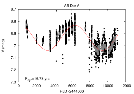
Figure 5: The $V_{\rm med}$ time-series for the AB Dor A. The grey squares are used to mark the $V_{\rm med}$ values computed in the 50-days segments.

The use of the activity indexes time-series allowed also the detection of secondary cycles with lengths of 400 d, 190 d and 90 d, respectively.

longtablelllllll List of the cycles detected in the present work
Target ID $P_{\rm cyc}$ Err FAP Meth. Act. Ind Mult.
(days) (days) %
continued.
Target ID $P_{\rm cyc}$ Err FAP Meth. Act. Ind Mult.
(days) (days) %
ASAS J001353-7441.3 1600 212 ¡ 0.01 PDM M I
ASAS J002409-6211.1 1025 52 0.07 PDM AM I
ASAS J002409-6211.1 390 - V M II
ASAS J002409-6211.1 190 - V A III
ASAS J002409-6211.1 100 - - V P IV
ASAS J003451-6155.0 ¿3000 - - V M I
ASAS J003451-6155.0 360 - - V M II
ASAS J003451-6155.0 290 - - V A III
ASAS J011315-6411.6 1801 161 ¡ 0.01 LS M I
ASAS J011315-6411.6 1428 172 ¡ 0.01 PDM A II
ASAS J011315-6411.6 290 - - V A III
ASAS J015749-2154.1 ¿3000 – – V M I
ASAS J020136-1610.0 615 35 0.08 PDM A I
ASAS J020136-1610.0 336 9 0.1 LS M II
ASAS J020718-5311.9 ¿3000 – – V M I
ASAS J020718-5311.9 1052 812 ¡ 0.01 PDM P II
ASAS J024126+0559.3 1249 362 0.04 PDM AM I
ASAS J024233-5739.6 190 - - V A II
ASAS J033049-4555.9 1081 80 ¡ 0.01 PDM A I
ASAS J033156-4359.2 ¿3000 – – V A I
ASAS J033156-4359.2 930 42 0.09 PDM M II
ASAS J045935+0147.0 1597 300 ¡ 0.01 PDM AM I
ASAS J050047-5715.4 1666 192 ¡ 0.01 PDM M I
ASAS J050047-5715.4 1142 134 ¡ 0.01 PDM A II
ASAS J050047-5715.4 380 - - V M III
ASAS J050651-7221.2 1081 80 ¡ 0.01 PDM AM I
ASAS J052845-6526.9 ¿3000 - - V M I
ASAS J052845-6526.9 400 - - V A II
ASAS J052845-6526.9 190 - - V MP III
ASAS J052845-6526.9 90 - - V A IV
ASAS J053705-3932.4 1052 50 0.01 PDM M I
ASAS J053705-3932.4 370 - - V A II
ASAS J053705-3932.4 290 - - V M III
ASAS J055329-8156.9 1290 56 0.04 PDM M I
ASAS J055329-8156.9 530 - - V A II
ASAS J055329-8156.9 400 - - V M III
ASAS J055329-8156.9 330 - - V AM IV
ASAS J055329-8156.9 135 - - V P V
ASAS J055751-3804.1 1379 102 0.03 PDM M I
ASAS J055751-3804.1 95 - - V P II
ASAS J060834-3402.9 1333 202 ¡ 0.01 PDM AM I
ASAS J061828-7202.7 ¿3000 – – V M I
ASAS J062607-4102.9 1538 138 0.07 PDM M I
ASAS J062806-4826.9 1250 117 0.02 PDM AM I
ASAS J063950-6128.7 429 13 0.09 LS A I
ASAS J064346-7158.6 ¿3000 - - V M I
ASAS J064346-7158.6 95 - - V P II
ASAS J070030-7941.8 1835 205 0.05 LS M I
ASAS J070030-7941.8 250 - - V AMP II
ASAS J070030-7941.8 150 - - V P III
ASAS J070153-4227.9 1835 173 ¡ 0.01 LS A I
ASAS J070153-4227.9 606 48 ¡ 0.01 PDM P II
ASAS J070153-4227.9 290 - - V A III
ASAS J070153-4227.9 230 - - V A IV
ASAS J072124-5720.6 1156 78 ¡ 0.01 LS AM I
ASAS J072124-5720.6 190 - - V A II
ASAS J072124-5720.6 160 - - V P III
ASAS J072822-4908.6 1600 157 0.06 PDM A I
ASAS J072851-3014.8 1904 275 ¡ 0.01 PDM A I
ASAS J072851-3014.8 1379 105 0.03 PDM M II
ASAS J073547-3212.2 1069 65 ¡ 0.01 LS M I
ASAS J082406-6334.1 ¿3000 – - V M I
ASAS J082406-6334.1 290 - - V M II
ASAS J082406-6334.1 240 - - V AM III
ASAS J082844-5205.7 1905 226 0.03 PDM A I
ASAS J083656-7856.8 ¿3000 – - V M I
ASAS J083656-7856.8 280 - - V M II
ASAS J083656-7856.8 235 - - V A III
ASAS J083656-7856.8 170 - - V AP IV
ASAS J083656-7856.8 130 - - V P V
ASAS J084006-5338.1 1905 194 0.08 PDM M I
ASAS J084200-6218.4 1333 123 ¡ 0.01 PDM M I
ASAS J084200-6218.4 90 - - V P II
ASAS J084229-7903.9 ¿3000 - - V M I
ASAS J084229-7903.9 420 - - V M II
ASAS J084229-7903.9 220 - - V A III
ASAS J084300-5354.1 ¿3000 - - V M I
ASAS J084300-5354.1 360 - - V M II
ASAS J084300-5354.1 200 - - V M III
ASAS J084432-7846.6 1481 96 ¡ 0.01 PDM M I
ASAS J084432-7846.6 220 - - V A II
ASAS J084432-7846.6 170 - - V A III
ASAS J084708-7859.6 400 - - V M I
ASAS J084708-7859.6 305 - - V AM II
ASAS J085156-5355.9 1587 143 ¡ 0.01 LS M I
ASAS J085156-5355.9 320 - - V A II
ASAS J085929-5446.8 590 27 0.1 LS A I
ASAS J085929-5446.8 438 10 ¡ 0.01 LS P II
ASAS J085929-5446.8 290 - - V M III
ASAS J085929-5446.8 150 - - V A IV
ASAS J092854-4101.3 1600 164 0.02 PDM M I
ASAS J094247-7239.8 1156 80 0.04 LS M I
ASAS J095558-6721.4 1333 114 ¡ 0.01 PDM M I
ASAS J095558-6721.4 365 - - V M II
ASAS J105351-7002.3 1599 426 ¡ 0.01 PDM M I
ASAS J105749-6914.0 1639 160 0.02 LS M I
ASAS J105749-6914.0 394 9 ¡ 0.01 V A II
ASAS J110914-3001.7 1489 110 ¡ 0.01 PDM AM I
ASAS J112117-3446.8 1250 138 ¡ 0.01 PDM AM I
ASAS J112117-3446.8 70 - - V A II
ASAS J112205-2446.7 1600 196 0.01 PDM AM I
ASAS J115942-7601.4 1250 112 ¡ 0.01 PDM A I
ASAS J115942-7601.4 697 32 0.08 LS M II
ASAS J115942-7601.4 75 - - V A III
ASAS J121531-3948.7 1666 164 ¡ 0.01 PDM A I
ASAS J121531-3948.7 1250 84 0.06 PDM M II
ASAS J121531-3948.7 55 - - V P III
ASAS J122034-7539.5 913 37 ¡ 0.01 LS A I
ASAS J122105-7116.9 2000 350 ¡ 0.01 PDM A I
ASAS J122105-7116.9 400 7 ¡ 0.01 LS M II
ASAS J123921-7502.7 1219 77 0.02 LS A I
ASAS J123921-7502.7 365 - - V M II
ASAS J125826-7028.8 1198 81 ¡ 0.01 LS M I
ASAS J125826-7028.8 833 36 0.07 PDM A II
ASAS J125826-7028.8 80 - - V A III
ASAS J134913-7549.8 1999 240 ¡ 0.01 PDM M I
ASAS J171726-6657.1 1904 205 0.08 PDM A I
ASAS J181952-2916.5 615 43 ¡ 0.01 PDM A I
ASAS J181952-2916.5 90 - - V P II
ASAS J184653-6210.6 1999 712 ¡ 0.01 PDM A I
ASAS J185306-5010.8 1136 87 0.07 LS AM I
ASAS J200724-5147.5 930 91 ¡ 0.01 PDM AM I
ASAS J204510-3120.4 1428 283 ¡ 0.01 PDM M I
ASAS J204510-3120.4 1176 171 0.01 PDM AM II
ASAS J205603-1710.9 1176 220 ¡ 0.01 PDM AM I
ASAS J205603-1710.9 394 11 0.03 LS M II
ASAS J212050-5302.0 1315 118 0.1 LS M I
ASAS J214430-6058.6 1600 166 0.04 PDM A I
ASAS J232749-8613.3 629 24 0.1 LS M I
ASAS J232749-8613.3 300 - - V M II
ASAS J232749-8613.3 265 - - V A III
ASAS J232749-8613.3 165 - - V A IV
ASAS J232749-8613.3 85 - - V AP V
ASAS J233231-1215.9 1695 259 0.1 LS M I
ASAS J234154-3558.7 1739 268 0.1 PDM A I

5 Discussion

5.1 Relationships between the cycle length, the rotation period and the Rossby number

Since stellar activity cycles were first detected, a relationship has been searched between the cycle period $P_{\rm cyc}$ and the stellar rotation period $P_{\rm rot}$. Böhm-Vitense (2007) analyzed a sample of stars obtained by selecting the best quality spectrophotometric data collected at Mt. Wilson. She identified three different stellar sequences that have an almost constant ratio $\frac{P_{\rm cyc}}{P_{\rm rot}}$. The Aa and the Ab sequences (where A stands for active) consist of young and active stars. The ratio $\frac{P_{\rm cyc}}{P_{\rm rot}}$ is between 400 and 500 for the Aa stars and it is about 300 for the Ab stars. The I sequence (where I stands for inactive) comprises old and less active stars for which the ratio $\frac{P_{\rm cyc}}{P_{\rm rot}}$ is about 90. Böhm-Vitense (2007) speculates that the three sequences are due to different kind of dynamos excited by different phenomena. According to her interpretation, the dynamo should be generated by SDR in A sequence stars and by a vertical shear in I sequence stars.

In Fig. 6 we plot the cycle lengths vs. the stellar rotation periods as in Böhm-Vitense (2007). The filled circles mark the primary cycles and the empty the secondary ones. We also over-plotted the three sequences identified by Böhm-Vitense (2007) and a fourth line corresponding to the $P_{\rm cyc}/P_{\rm rot}\simeq 5$ ratio of the solar Rieger cycle. The figure shows that the primary cycles do not follow any particular trend and that their lengths seem to be uncorrelated with the rotation periods. The secondary cycles are also uniformly distributed between the Ab and the I sequences and do not follow any particular pattern. Some of the secondary cycles lie beneath the I sequence and their $P_{\rm cyc}/P_{\rm rot}$ ratio is very close to that of the solar Rieger-cycle.

Other authors (see e.g. Baliunas et al. 1996; Vida et al. 2014; Oláh et al. 2016) searched for a correlation between $\frac{P_{\rm cyc}}{P_{\rm rot}}$ and the parameter $\frac{1}{P_{\rm rot}}$ that, according to Baliunas et al. (1996), should be proportional to the dynamo number D. In these works a linear fit is performed of investigating the relationship between the logarithms of the two quantities. The slope $m$ extracted from the linear fit is the exponent of the power law $P_{\rm cyc}/P_{\rm rot}=(1/P_{\rm rot})^{m}$. If $m$ is close to 1 then no correlation exists between $P_{\rm cyc}$ and $P_{\rm rot}$. Baliunas et al. (1996) found m=0.74 that is in agreement with the value m=0.76 recently found by Oláh et al. (2016).

In Fig. 7 we plotted $\rm log\frac{P_{\rm cyc}}{P_{\rm rot}}$ vs. $\rm log\frac{1}{P_{\rm rot}}$ for our targets. We performed a linear fit between the two quantities and we found $m=1.02\pm 0.06$ that indicates no correlation between $P_{\rm cyc}$ and $P_{\rm rot}$. Our results are sligthly higher than those found by Baliunas et al. (1996) and Oláh et al. (2016) but are in close agreement with those found by Savanov (2012) and Lehtinen et al. (2016).

The lack of correlation between $P_{\rm cyc}$ and $P_{\rm rot}$ seen in Fig. 6 and in Fig. 7 suggests that the dynamo mechanism occurring in our young targets stars is different from that acting in the older Mt. Wilson stars selected by Böhm-Vitense (2007) .

The lack of correlation between $P_{\rm cyc}$ and $P_{\rm rot}$ seen in our targets could be related to their low Rossby number values. In fact, most of our targets are fast rotating stars ($P_{\rm rot}$ ¡ 10 d) with Ro values falling in the range (0.004-0.17) and $Ro_{\rm Br}$ values in the range (0.002-0.06). These ranges are very different from those covered by the Mt. Wilson stars. Saar & Brandenburg (1999) extended the sample of the Mt. Wilson stars with an ensemble of young and fast rotating stars and showed that these stars formed a third branch in the ($\rm log\frac{P_{\rm rot}}{P_{\rm cyc}}$,$\rm logRo_{\rm Br}^{-1}$) plane. This branch was called the Super Active branch and was clearly distinct from the Active and Inactive ones and was attributed to a different dynamo mechanism. Recently, Lehtinen et al. (2016) exploited long-term photometry to measure the cycle length $P_{\rm cyc}$ of 21 young active stars and found that the Active and the Super-Active branch are connected by a Transitional branch. In Fig. 8 we plotted the $\rm log\frac{P_{\rm rot}}{P_{\rm cyc}}$ values vs. the $\rm logRo_{Br}^{-1}$ values inferred for our stars. In the plot we reported also the data coming from Saar & Brandenburg (1999) and from Lehtinen et al. (2016). The primary cycles of our stars are in good agreement with the Transitional Sequence as defined by Lehtinen et al. (2016). Note that also Lehtinen et al. (2016) did not find any correlation between $P_{\rm cyc}$ and $P_{\rm rot}$ in their targets. Hence, we can conclude that in stars belonging to the Transitional Branch, the cycle length $P_{\rm cyc}$ and the rotation period $P_{\rm rot}$ are uncorrelated.

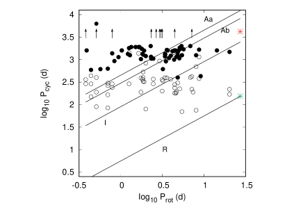
Figure 6: The $P_{\rm cyc}$ length vs. the stellar rotation period $P_{\rm rot}$. The filled circles mark the primary cycles and the empty circles the secondary ones. The arrows mark the stars for which the visual inspection of time-series revealed $P_{\rm cyc}\geq 3000d$. The continuous line, the dashed line and the dotted line represent the Aa, the Ab and the I sequences identified by Böhm-Vitense (2007), respectively. The dash-dotted line represents the locus where the $\frac{P_{\rm cyc}}{P_{\rm rot}}$ ratio is equal to the ratio between the typical length of the Rieger cycle and the solar rotation period. Red asterisk: solar Schwabe cycle. Green asterisk: solar Rieger cycle

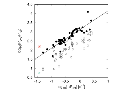
Figure 7: The $\frac{P_{\rm cyc}}{P_{\rm rot}}$ ratio vs. the inverse of the stellar rotation period. The filled circles mark the primary cycles and the empty mark the secondary ones. The slope $m=1.02\pm 0.06$ of the best-fitting straight line indicates a lack of correlation between $P_{\rm cyc}$ and $P_{\rm rot}$. Black asterisk: solar Schwabe cycle. Green asterisk: solar Rieger cycle

5.2 Relationship between ${P_{\rm cyc}}$ and global stellar parameters

We investigated how the cycle lengths $P_{\rm cyc}$ are related to the global stellar parameters of our targets. We evaluated the degree of the correlation between $P_{\rm cyc}$ and a given parameter by computing the Spearman rank-order correlation coefficient ($r_{S}$) (Press et al. 1992). This coefficient is a non-parametric measure of the monotonicity of the relationship between two datasets.

A value of $r_{S}$ close to 0 implies that the two datasets are poorly correlated, whereas the closer $r_{S}$ is to $\pm 1$ the stronger the monotonic relationship between the two variables.

The statistical significance of a given value $r_{S}=r_{0}$ can be evaluated by computing the two sided p-value i.e. the probability $(P(|r_{S}|\geq|r_{0}|)$ under the null hypothesys that two invesigated datasets are non-monotonically correlated (Press et al. 1992)

In Table 2 we reported the Spearman correlation coefficients between the length $P_{\rm cyc}$ of the primary cycles and the different stellar parameters. The corresponding p-values are alo reported. The values of $|r_{S}|$ are very close to 0 in all the cases indicating a poor correlation between $P_{\rm cyc}$ and the different variables.

5.3 Relationship between ¡IQR¿ and global stellar parameters

As remarked in Sec. 2, the IQR index is proportional to the amplitude of the rotational modulation signature and is related to the non-axisymmetric part of the spot distribution. The amplitude of rotational modulation is a widely used activity index and can be regarded as a robust proxy of the surface magnetic activity. García et al. (2013) demonstrated that the variance of the Total Solar Irradiance, computed on a 60-d sliding window, closely mimics the variations of the 10.7 cm radio flux that in turn is a good indicator of the solar magnetic activity (see Bruevich et al. 2014, for details). We computed the Spearman coefficient between ¡IQR¿ and different stellar parameters in order to investigate how the mean level of the stellar surface magnetic activity is linked to the stellar properties. In Table 3 we reported the values of $r_{\rm S}$ for the different parameters. In this case, $r_{\rm S}$ values are significantly higher then those computed for $P_{\rm cyc}$. A good correlation ($|r_{\rm S}|\simeq 0.5$ is seen between ¡IQR¿ and $T_{\rm eff}$, $\tau_{\rm C}$, $\tau_{\rm diff}$, $R_{\rm C}$ and $D_{\rm{\rm N}}$. The sign of correlation is positive for $\tau_{\rm C}$, $\tau_{\rm diff}$ and $D_{\rm N}$ and negative for $T_{\rm eff}$ and $R_{\rm C}$.

In Fig. 9 we reported ¡IQR¿ vs. the different stellar parameters for which a significant correlation is seen ($r_{\rm S}\simeq 0.5$ ). Despite the scatter in the data, the different plots clearly show that ¡IQR¿ tends to increase with $\tau_{\rm diff}$, $\tau_{\rm C}$ and $T_{\rm eff}$ and it has a negative correlation with $T_{\rm eff}$ and $R_{\rm C}$ .

A weaker but still significant correlation is also seen between ¡IQR¿ and the photometric shear $\Delta\Omega_{\rm phot}$. In Fig. 10 we plotted ¡IQR¿ vs. $\Delta\Omega_{\rm phot}$. The different stars are color-coded according to their effective temperature $T_{\rm eff}$. The plot shows that:

• $\Delta\Omega_{\rm phot}$ tends to increase with temperature (as demonstrated in Paper I)

• the sign of the correlation between ¡IQR¿ and $\Delta\Omega_{\rm phot}$ and ¡IQR¿ is negative ($r_{S}=-0.43$). This means that the lower $\Delta\Omega_{\rm phot}$ the higher ¡IQR¿.

These results are in very good agreement with the theoretical models developed by Kitchatinov & Olemskoy (2011). In fact, these models predict that even a small surface differential rotation is very efficient for dynamos in M-type stars, it is less efficient in K- and G- type and even a strong differential rotation is inefficient in F type stars.

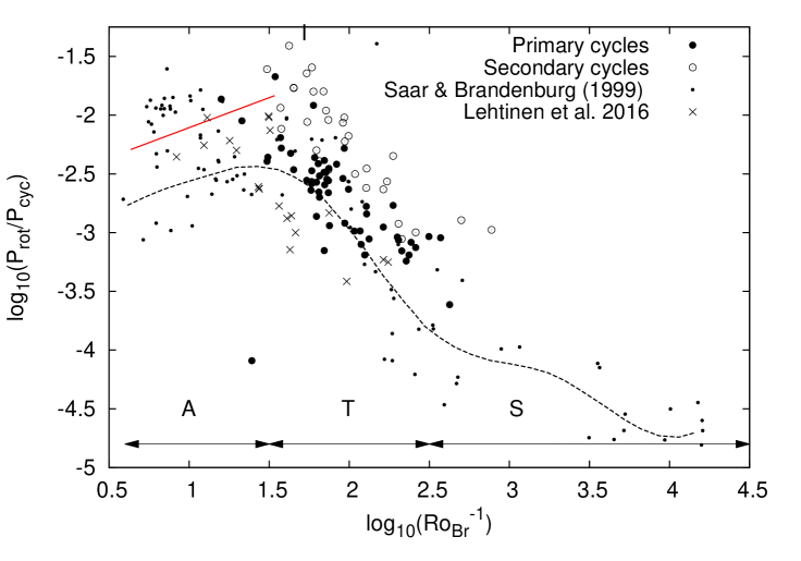
Figure 8: The $\frac{P_{\rm cyc}}{P_{\rm rot}}$ ratio vs. the $Ro_{\rm Br}$ number. The filled bullets mark the primary cycles whereas the empty bullets the secondary ones. The black points and the black crosses mark the results by Saar & Brandenburg (1999) and Lehtinen et al. (2016), respectively. The red continuous line depicts the Inactive Sequence. The black dotted line depicts the curve inferred by Lehtinen et al. (2016) and connects the Active, the Transitional and the Super-Active sequence. The $Ro_{\rm Br}$ ranges corresponding to the three sequences are marked with the black arrows and labelled with A, T, and S, respectively.

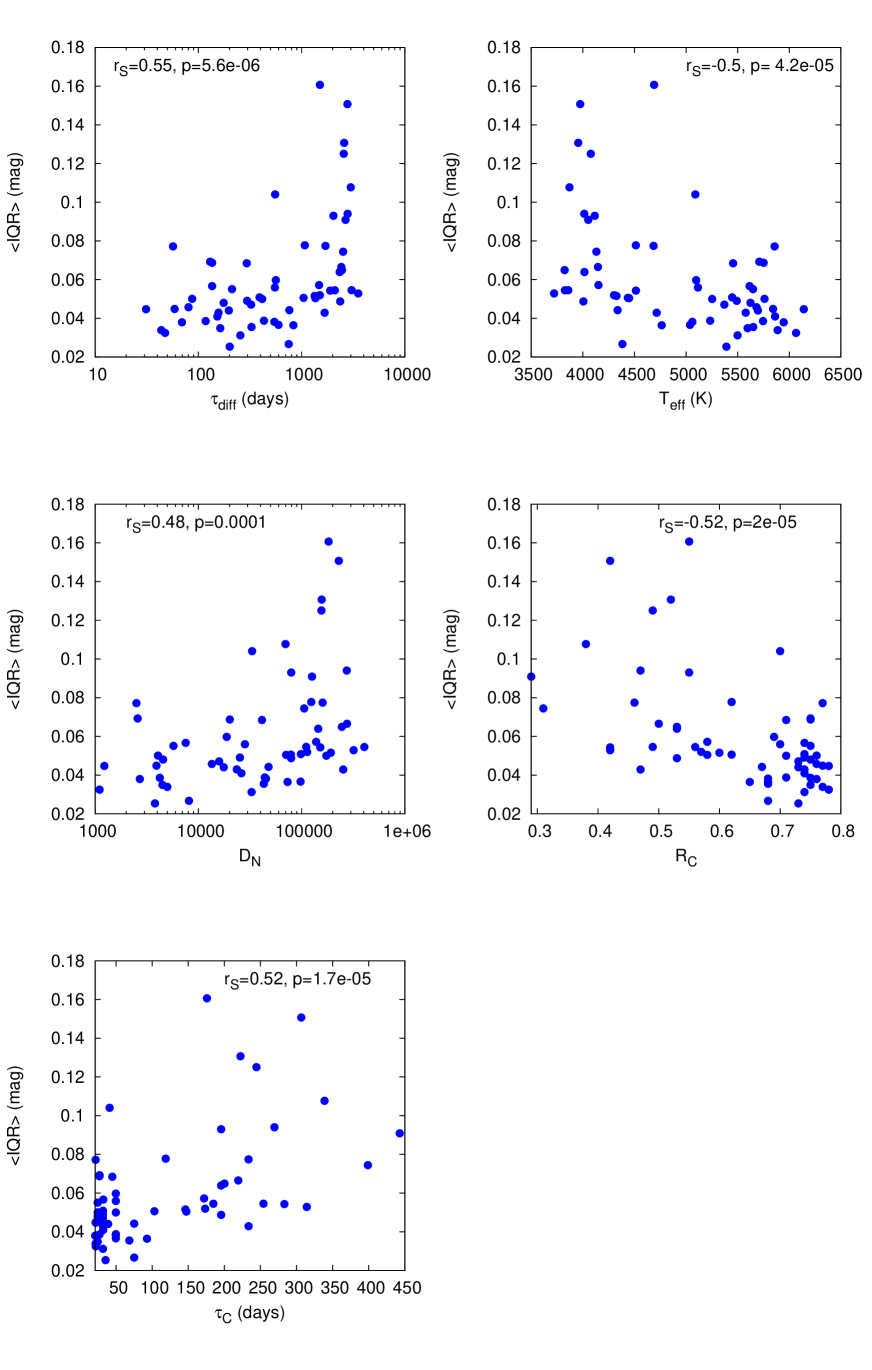
Figure 9: In the different panels we reported ¡IQR¿ vs. the parameters $\tau_{\rm diff}$, $T_{\rm eff}$, $D_{\rm N}$, $R_{\rm C}$ and $\tau_{\rm C}$, respectively. In each panel we also reported the Spearman coefficient $r_{\rm S}$ and the corresponding two-sided p-value.

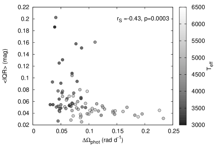
Figure 10: ¡IQR¿ vs. $\Delta\Omega_{\rm phot}$. The points are color coded according the stellar effective temperature $T_{\rm eff}$.

Table 2: Spearman correlation coefficient between $P_{\rm cyc}$ and different stellar parameters. The parameters are ordered by decreasing $|r_{S}|$.

Parameter	$r_{S}$	p
$P_{\rm rot}$	0.16	0.25
$\Delta\Omega_{\rm phot}$	-0.10	0.48
$D_{\rm N}$	-0.10	0.47
$\tau_{\rm C}$	0.04	0.79
$R_{\rm C}$	-0.04	0.76
Ro	0.03	0.84
$T_{\rm eff}$	-0.03	0.86
age	0.02	0.86
$\tau_{\rm diff}$	0.01	0.95

Table 3: Spearman correlation coefficient $r_{S}$ between ¡IQR¿ and different stellar parameters. The parameters are ordered by decreasing $|r_{S}|$.

Parameter	$r_{S}^{\prime}$	p
$\tau_{\rm diff}$	0.55	5.6e-06
$\tau_{\rm C}$	0.52	1.7e-05
$R_{\rm C}$	-0.52	2e-05
$T_{\rm eff}$	-0.50	4.2e-05
$D_{\rm N}$	0.48	0.0001
$\Delta\Omega_{\rm phot}$	-0.43	0.0003
age	-0.39	0.001
Ro	-0.35	0.0061
$P_{\rm rot}$	0.29	0.018
$P_{\rm cyc}$	0.08	0.56

5.4 Evolution of $P_{\rm cyc}$ and ¡IQR¿ with the stellar age

Oláh et al. (2016) investigated how the $\frac{P{\rm cyc}}{P_{\rm rot}}$ ratio depends on the stellar age. They found that $\frac{P_{\rm cyc}}{P_{\rm rot}}$ exhibits a large scatter in the younger and more active stars of their sample whereas the older stars have about the same value. The age at which $\frac{P_{\rm cyc}}{P_{\rm rot}}$ becomes constant is, according to their work, at about 2.2 Gyr, i.e. the age of the Vaughan-Preston gap (Vaughan & Preston 1980). The sample of stars analyzed by Oláh et al. (2016) covers the age range 200-6200 Myr. Our work permits us to extend the age range studied by Oláh et al. (2016) and to investigate the transition age between the PMS and the MS phase. Our analysis is slightly different from that performed by Oláh et al. (2016). We decided to investigate the relationship between $P_{\rm cyc}$ and the stellar age instead of the relationship between $\frac{P_{\rm cyc}}{P_{\rm rot}}$ and the stellar age. In fact, the trend of the between $\frac{P_{\rm cyc}}{P_{\rm rot}}$ ratio, in the age range covered by our targets, could be dominated by the complex $P_{\rm rot}$ evolution seen in the PMS stars (see e.g. Lanzafame & Spada 2015, and references therein). In the top panel of Fig. 11, we reported the length of the primary cycles $P_{\rm cyc}$ vs. the stellar age. The blue filled symbols mark the cycles identified in the present work and the red empty symbols mark those found by Oláh et al. (2016). The picture shows that $P_{\rm cyc}$ is about constant in the age range $4-300\leavevmode\nobreak\ \rm Myr$. After 300 Myr, the cycle lengths are more scattered and seem to increase with the stellar age. After 2.2 Gyr, that is the age corresponding to the Vaughan-Preston gap, the scatter in $P_{\rm cyc}$ decreases as described by Oláh et al. (2016). Note that, although our data cover an interval of about 3000 d which could prevent the detection of longer cycles, we observed long-term trends suggesting cycles longer than 3000 d just in 11 of the 90 investigated targets. For this reason, we are confident that our data are not seriously affected by a selection bias and that the age range investigated here is really, on average, characterized by cycles shorter than those observed in the older Mt. Wilson stars. In the bottom panel of Fig. 11 we plotted ¡IQR¿ vs. the stellar age. The picture shows that ¡IQR¿ tends to decrease with the stellar age as also indicated by the Spearman coefficient $r_{\rm S}=0.39$. This result is in agreement with all the works that studied the evolution of the level of magnetic activity vs. age (see e.g. Žerjal et al. 2017; Oláh et al. 2016, and references therein)

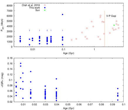
Figure 11: Top panel. $P_{\rm cyc}$ vs. the stellar age. The blue filled circles refer to the primary cycles detected in the present work and the red empty circles to the data reported by Oláh et al. (2016). The blue arrows mark the stars for which the visual inspection of time-series revealed $P_{\rm cyc}\geq 3000\leavevmode\nobreak\ d$. Bottom panel. The activity index ¡IQR¿ vs. the stellar age.

5.5 Butterfly diagrams

In the Sun, the latitudes at which ARs occur change vs. time according to the so-called “butterfly-diagram”. At the beginning of a solar cycle, ARs emerge in belts located at intermediate latitudes ($\pm 35\deg$). As the cycle progresses, the ARs formation regions migrate toward the equator. At the beginning of the next cycle, the ARs form again at intermediate latitudes. The solar SDR combined with the ARs migration determines a decrease in the rotation period detectable along the 11-yr cycle because the ARs located at intermediate latitudes rotate slower than those located at the equator. As remarked in Paper I and in Sec. 2.2, the Activity Index $P_{\rm rot}$ of a given star can therefore be regarded as a tracer of the ARs migration in latitude. This Activity Index cannot give information about the exact latitudes at which ARs occur but can give insight about the nature of stellar magnetic field. In fact, in a star with a solar-like dynamo, we expect that the trend of $P_{\rm rot}$ with time mimics that of the solar butterfly diagram i.e. that, during a given cycle, $P_{\rm rot}$ decreases in time and that it rises rapidly to higher values at the beginning of the next cycle. Messina & Guinan (2003), for instance, analyzed the trend of $P_{\rm rot}$ in six young solar analogues. They noticed that three of these stars follow a solar behaviour whereas the other three show an anti-solar behaviour with $P_{\rm rot}$ increasing during the cycle. The $P_{\rm rot}$ time-series of our target stars have in general less points than the $V_{\rm med}$ and IQR time-series. Indeed, as remarked in Paper I, $P_{\rm rot}$ is detectable in a given time interval only if ARs maintain a stable configuration. In Fig. 12 and 13 we reported the $P_{\rm rot}$ time-series for the stars ASAS J070030-7941.8 and ASAS J055329-8156.9 that are the targets with the highest number of $P_{\rm rot}$ determinations. The $V_{\rm med}$ time-series and the IQR time-series of the two stars are also reported for comparison. The stars have two primary cycles with length $P_{\rm cyc}\leavevmode\nobreak\ =1834\leavevmode\nobreak\ d$ and $P_{\rm cyc}\leavevmode\nobreak\ =1290\leavevmode\nobreak\ d$, respectively. The two sinusoids best-fitting the data and corresponding to the primary cycles are over-plotted on the $V_{\rm med}$ time-series. The visual inspection of the pictures shows that in both stars:

• The $P_{\rm rot}$ index oscillates with a cycle shorter than the primary cycle; hence the ARs latitude migration occurs in a time-scale shorter than the length of the primary cycle;

• in some intervals, the trend of $P_{\rm rot}$ vs time mimics the trends of $V_{\rm med}$ and IQR and the maxima and minima of $P_{\rm rot}$ correspond to local maxima and minima of the $V_{\rm med}$ and $IQR$ time-series; in other intervals the maxima and minima of $P_{\rm rot}$ are uncorrelated with those of the $V_{\rm med}$ and IQR time-series. This implies that in some time intervals the changes in AR latitudes are correlated with the variations in the ARs areas and in the mean level of magnetic activity whereas in some other intervals there is no correlation;

• the $P_{\rm rot}$ variations with time are very different from those occurring in the Sun. Rise patterns are followed by decreasing patterns. This implies that ARs first migrate from regions with shorter rotation periods to regions with higher rotation periods and then migrate in the opposite sense. In the Sun the migration occurs in only one sense i.e. from the intermediate latitudes to the equator.

Similar trends are observed in all the targets analyzed here.

The patterns seen in the $P_{\rm rot}$ time-series of our targets can be regarded as a further evidence that the dynamo acting in these stars is very different from that acting in the Sun.

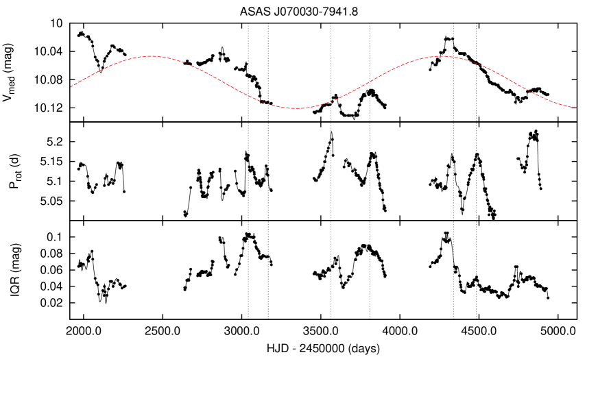
Figure 12: Top panel: the $V_{\rm med}$ time-series for the star ASAS J070030-7941.8. Mid panel; the $P_{\rm rot}$ time-series. Bottom panel: the IQR time-series. A primary cycle with length $P_{\rm cyc}=1834\leavevmode\nobreak\ d$ was detected in the $V_{\rm med}$ time-series and the sinusoid best-fitting the data was over-plotted on it (red dashed line). The $P_{\rm rot}$ and the IQR time-series exhibit cycles (dark continuous lines) shorter than the primary one. The black dotted lines mark the times at which maxima occur in the $P_{\rm rot}$ time-series.

6 Conclusions

In the present work we searched for activity cycles in stars belonging to young loose stellar associations. We analyzed the long-term time-series of three different activity indexes and we were able to detect activity cycles in 67 stars and to measure their length $P_{\rm cyc}$. We investigated how $P_{\rm cyc}$ is correlated with global stellar parameters by computing the Spearman coefficient $r_{\rm S}$ between $P_{\rm cyc}$ and the different parameters. We investigated how activity cycles evolve with the stellar age. In particular, our work extends the age range covered by the Mt Wilson stars whose properties have been recently reanalyzed by Oláh et al. (2016). Our analysis led to the following results:

1. most of the analyzed stars show multiple and complex cycles according to the results found by Oláh et al. (2016) for young and active stars;

2. some of the detected secondary cycles have a $\frac{P_{\rm cyc}}{P_{\rm rot}}$ ratio similar to that of the solar Rieger-cycles ($\frac{P_{\rm cyc}}{P_{\rm rot}}\simeq\leavevmode\nobreak\ 5$);

3. the location of our targets in the $\rm log\frac{P_{\rm cyc}}{P_{\rm rot}}-\rm logRo_{\rm Br}^{-1}$ plane is in good agreement with the Transitional branch as defined by Lehtinen et al. (2016);

4. the cycle length $P_{\rm cyc}$ is uncorrelated with the stellar rotation period $P_{\rm rot}$ in our targets; this result confirms that found by Lehtinen et al. (2016) for stars belonging to the Transitional Branch;

5. $P_{\rm cyc}$ is essentially uncorrelated with global stellar parameters in the age range we investigated;

6. the activity index ¡IQR¿, that can be regarded as a proxy of the magnetic surface activity level, is positively correlated with $\tau_{\rm C}$, $\tau_{\rm diff}$, $D_{\rm N}$ and negatively correlated with $T_{\rm eff}$ and$R_{\rm C}$;

7. in agreement with the Kitchatinov & Olemskoy (2011) model, even a small differential rotation is efficient for dynamos in M-type stars, but it becomes less efficient or completely inefficient at increasing $T_{\rm eff}$;

8. the analysis of the butterfly diagrams of our target stars shows that:

   • the ARs migration in latitude occurs over a time-scale shorter than the primary cycle;

   • the latitudes at which ARs emerge seem to oscillate from a maximum to a minimum latitude and vice-versa. This is very different from the solar behaviour where the spots migrate only from intermediate latitudes to the equator;

9. we merged our data with those analyzed by Oláh et al. (2016) and we studied the trend of $P_{\rm cyc}$ vs. the stellar age in the range (0.004-9 Gyr); we found that $P_{\rm cyc}$ is about constant and does not show significant correlation with the stellar age in the range ($4-300\rm Myr$); after 300 Myr $P_{\rm cyc}$ values are quite scattered and tend to increase with the stellar age; after 2.2 Gyr, $P_{\rm cyc}$ values tend to be less scattered and seem to converge to the solar value as described by Oláh et al. (2016);

10. the activity index ¡IQR¿ decreases with the stellar age in the age range 4-95 Myr;

11. merging the ASAS time-series of the star AB Dor A with the photometric data from previous works and we detected a cycle with length $P_{\rm cyc}=16.78\pm 2\rm yr$ and shorter secondary cycles with lengths of 400 d, 190 d, and 90 d.

Appendix A Effect of the sliding-window algorithm on a periodic signal.

The segmentation procedure used to derive activity indexes is equivalent to a low-pass filter. This preserves the signals with a frequency lower than a certain cutoff frequency and attenuates signals with frequencies higher than the cutoff frequency. In our case, the use of a sliding-window with length T=100 d attenuates signals with periods shorter than 100-d but, in some cases, does not completely suppress them. We performed different tests by simulating sinusoidal signals with different amplitudes and periods and by processing them with our segmentation algorithm. In the top panel of Fig. 14 we plotted a simulated time-series obtained by combining two sinusoidal signals with periods $\rm P_{1}=300\rm d$, $\rm P_{2}=45\rm d$ and amplitudes $\rm A_{1}=0.4$, $\rm A_{2}=0.6$, respectively. A white gaussian noise with variance $\sigma=0.1$ was added to the simulated data. In the bottom panel, we plotted the filtered signal obtained after processing the simulated time-series with our segmentation algorithm. The filter has attenuated but not suppressed the 45-d signal. In Fig. 15 we reported a similar test obtained by combining two period signals $\rm P_{1}=300\rm d$, $\rm P_{2}=45\rm d$ and amplitudes $\rm A_{1}=0.4$, $\rm A_{2}=0.1$. In this second case the signal with $\rm P=45\rm d$ is completely suppressed.

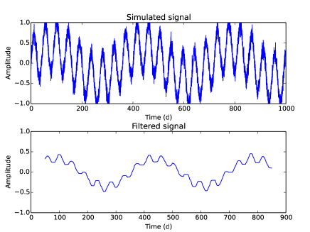
Figure 14: Top panel. A simulated time-series obtained by combining two sinusoidal signals with periods $\rm P_{1}=300\rm d$, $\rm P_{2}=45\rm d$ and amplitudes $\rm A_{1}=0.4$, $\rm A_{2}=0.6$, respectively. Bottom panel. Filtered time-series. The segmentation algorithm attenuates but does not suppress the signal with P = 45 d.

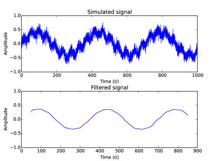
Figure 15: Top panel. A simulated time-series obtained by combining two period signals with periods $\rm P_{1}=300\rm d$, $\rm P_{2}=45\rm d$ and amplitudes $\rm A_{1}=0.4$, $\rm A_{2}=0.1$, respectively. Bottom panel. Filtered time-series. The 45-d is completely suppressed in this case.