Time series experiments and causal estimands:
exact randomization tests and trading

Abstract

We define causal estimands for experiments on single time series, extending the potential outcome framework to dealing with temporal data.  Our approach allows the estimation of a broad class of these estimands and exact randomization based $p$-values for testing causal effects, without imposing stringent assumptions.  We further derive a general central limit theorem that can be used to conduct conservative tests and build confidence intervals for causal effects.  Finally, we provide three methods for generalizing our approach to multiple units that are receiving the same class of treatment, over time.  We test our methodology on simulated “potential autoregressions,”which have a causal interpretation.  Our methodology is partially inspired by data from a large number of experiments carried out by a financial company who compared the impact of two different ways of trading equity futures contracts.  We use our methodology to make causal statements about their trading methods.

Keywords: Causality, potential outcomes, trading costs, non-parametric.

1 Introduction

In longitudinal experiments with time-varying exposure causal estimands are traditionally defined as averages over a population.  Population averaging usually requires that the number of units in the experiment exceed the duration of the study.  However, there are applications where the length of the experiment is greater than the number of units.  The most extreme case is when there is only one unit that is being experimented on over time.  We refer to this as a “time series experiment.”  For time series experiments, the usual population estimands fail to capture the personalized nature of the problem and are virtually impossible to estimate without imposing strong, often unrealistic, assumptions.

In this paper, we generalize the standard one-period experimental treatments on multiple units setup to a multiple-period experimental treatment path carried out on a single unit.  Our time series experiments have at their heart potential outcome paths, allowing us to define unit level causal estimands.  We define a broad class of causal effects and show how to estimate several key examples under a relatively weak non-anticipating treatments assignment assumption.  For these causal effects, we derive two non-parametric inferential strategies based on the randomization alone.  One of these strategies delivers an exact randomization test of no causality in time series.  We then generalize our results to the setting with multiple units.

Our methods are partially inspired by our analysis of a database of experiments carried out by AHL Partners LLP (London, UK), a large quantitative hedge fund, who have been executing orders through both human traders and computer algorithms.  To quantify the relative performance of these two methods they have been running experiments, randomly allocating jobs to the human and the computer.  We will use our causal methods to make inference on the causal effect of these treatments on the relative costs of trading.  The data covers a year of experiments on 10 futures markets on equity indexes.

Our approach embraces the potential outcomes phrasing of experiments and causal inference, which has its origins in Neyman (1923), Kempthorne (1955), Cox (1958), Rubin (1974) and Robins (1986).  In Section 6 we will be precise about how our work relates to other studies of using temporal data to learn about causal effects.  In particular, we will discuss the work of, for example, Robins, et al, Murphy et al and Angrist, Kuersteiner et al as well as the many papers which have been published on impulse response functions, Granger causality, highly structured time series models and “natural” experiments.

This paper’s structure is as follows.  In Section 2, we define the potential outcome paths, the outcome path and the non-anticipating treatment path.  In Section 3, we define what we mean by causal effects and estimands.  In Section 4, we discuss experiments and using the results to estimate causal effects. In Section 5, we propose how to conduct inference on the causal effects using just the randomization in the treatment.  These methods are exact for any time series being treated so long as the treatment regime is non-anticipating.   In Section 6, we compare our causal effects and inference approaches with those familiar in the literature. In Section 7, we extend our time series results on a single unit to the case of multiple units each recorded through time.  In Section 8, we conduct some simulation experiments to see the effectiveness of our procedures focusing on what we call a potential autoregression.  In Section 9, we give our empirical illustration, measuring the causal effect of trading.  In Section 10, we give our concluding remarks.  The Appendix gathers some of the more technical proofs for the theorems and lemmas discussed in the main body of the text. The Web Appendix contains a practical description of how to conduct a randomization test, some more general theorems and extra figures.

2 The treatment path and potential outcome paths

At each time step, $t=1,\dots,T$, we will expose a single unit to either treatment, $W_{t}=1$, or control, $W_{t}=0$, and subsequently measure an outcome.  We focus on binary treatments; however, our results generalize to multiple treatments.  The random “treatment path” is

$$W_{1:t}=(W_{1},\dots,W_{t}).$$

We denote a realization of $W_{1:t}$ by $w_{1:t}$.

Figure 1: The left figure shows all the potential outcome paths for $T=3$. The right figure shows the observed outcome path $Y_{1:3}(w_{1:3})$ for $w_{1:3}=(1,1,0)$, indicated by the thick blue line. The gray arrows indicate the missing data.

In classical causal inference the treatment path is of length $1$, and each unit only has $2^{1}$ potential outcomes (the outcome that would be observed if the unit receives control and the outcome that would be observed if the unit receives treatment).  In a time series experiment, we follow a unit over time and administer $T$ different treatments.  At each time point $t$ the treatment path is of length $t$ and therefore there must be $2+2^{2}+...+2^{t}=2(2^{t}-1)$ potential outcomes up to time $t$ representing the $2^{t}$ different treatment paths that could be traversed.

Example 1

Suppose $T=3$. When $t=1$ there are $2^{1}=2$ potential outcomes $Y_{1}(0),Y_{1}(1)$, as the unit can either receive treatment $0$ or $1$. At time $t=2$, there are $2^{2}=4$ potential outcomes $Y_{2}(0,0),Y_{2}(0,1),Y_{2}(1,0),Y_{2}(1,1)$, as the unit can receive $\{0,0\}$, $\{0,1\}$, $\{1,0\}$ or $\{1,1\}$.  When $t=3$ there are $2^{3}=8$ potential outcomes, $Y_{3}(0,0,0)$, $Y_{3}(0,1,0)$, $Y_{3}(0,0,1)$, $Y_{3}(0,1,1)$, $Y_{3}(1,0,0)$, $Y_{3}(1,0,1)$, $Y_{3}(1,1,0)$, $Y_{3}(1,1,1)$, corresponding to all the possible values the treatment path could have taken.  The left hand side of Figure 1 depicts this.

The set of $2^{t}$ potential outcomes at time $t$, denoted by $Y_{t}(\bullet)$, are defined by

$$Y_{t}(\bullet)=\{Y_{t}(w_{1:t}):w_{1:t}\in\{0,1\}^{t}\},$$

so the potential outcomes at time $t$ only functionally depend upon current and past treatments.  This stops current potential outcomes depending upon future treatments.

The collection of all potential paths up to time $t$ is written as

$$Y_{1:t}(\bullet)=\left\{Y_{1}(\bullet),Y_{2}(\bullet),...,Y_{t}(\bullet)\right\},$$

containing $2(2^{t}-1)$ random variables. The potential path for the treatment path $w_{1:t}$ is

$$Y_{1:t}(w_{1:t})=\left\{Y_{1}(w_{1}),Y_{2}(w_{1:2}),...,Y_{t}(w_{1:t})\right\}.$$

Formulating treatments and potential outcomes as paths was introduced into longitudinal analysis by Robins (1986).  For binary time series it was used by Robins et al. (1999) in their Section 7, for state space models by Bondersen et al. (2015) and generally by Blackwell and Glynn (2016).

We do not make any assumptions on the dimension of $Y_{t}(w_{1:t})$.  In particular, nothing changes if the outcome contains both primary and secondary outcomes of interest.  Therefore without any loss of generality, we can assume that any covariates that are measured are unaffected by the experiment; otherwise, they would be considered as secondary outcomes.

Example 2

(continuing Example 1). The number of potential outcomes up to time $3$ is $14$. There are $2^{3}=8$ potential paths, e.g. $Y_{1:3}(1,1,1)=\left\{Y_{1}(1),Y_{2}(1,1),Y_{3}(1,1,1)\right\}$. In the experiment we observe one of these potential paths, the other seven will be missing.

Our framework is model free, but it helps intuition to consider an example.

Example 3

A first-order (vector) “potential autoregression” $Y_{1:T}(\bullet)$ holds when, for every permissible treatment path $w_{1:T}$, the potential outcomes follow the dynamic

$$Y_{t}(w_{1:t})=\mu(w_{1:t})+\phi\left(w_{1:t}\right)Y_{t-1}(w_{1:t-1})+\sigma(w_{1:t})\varepsilon_{t},\quad t=1,2,...,T,$$

where $\mu(\bullet)$, $\phi\left(\bullet\right)$ and $\sigma(\bullet)$ are non-stochastic. The treatment-invariant $\varepsilon_{1},...,\varepsilon_{T}$ couple the potential paths. When $\phi\left(w_{1:t}\right)=\phi$, $\mu(w_{1:t})=\mu+\sigma\mu(w_{t})$ and $\sigma(w_{1:t})=\sigma$ we label this an “impulse potential autoregression”.  Then $\mu(w_{1:t})+\sigma(w_{1:t})\varepsilon_{t}=\mu+\sigma\left\{\varepsilon_{t}+\mu(w_{t})\right\}$. A first order “potential moving average” $Y_{1:T}(\bullet)$ holds when

$$Y_{t}(w_{1:t})=\mu(w_{1:t})+\sigma(w_{1:t})\varepsilon_{t}+\theta(w_{1:t-1})\sigma(w_{1:t-1})\varepsilon_{t-1},\quad t=1,2,...,T,$$

where $\mu(\bullet)$, $\theta(\bullet)$ and $\sigma(\bullet)$ are non-stochastic. When $\theta(w_{1:t-1})=\theta$, $\mu(w_{1:t})=\mu+\sigma\mu^{\ast}(w_{t})+\sigma\mu^{\ast}(w_{t-1})$ and $\sigma(w_{1:t})=\sigma$, then we label this an “impulse moving average” $Y_{t}(w_{1:t})=\mu+\sigma\left\{\varepsilon_{t}+\mu^{\ast}(w_{t})\right\}+\theta\sigma\left\{\varepsilon_{t-1}+\mu^{\ast}(w_{t-1})\right\}$.  The right hand side of this only depends upon $w_{t-1:t}$, a special case of the m-dependent potential process discussed in Web Appendix B.2.   The autoregressive and moving average impulse models have a treatment which acts as an “impulse” for the innovation in the model à la Sims (1980).

The challenge of causal inference on time series is that we only observe one treatment path, $w_{1:T}^{\text{obs}}=(w_{1}^{\text{obs}},\dots,w_{T}^{\text{obs}})$, since we can only administer one treatment at each time step. After administering the treatment path the outcomes are $y_{1:T}^{\text{obs}}=(y_{1}^{\text{obs}},\dots,y_{T}^{\text{obs}})$.

To link the treatment and the outcome paths, we assume that there is only one version of the treatment, the treatment assigned is the treatment the unit is offered and receives. Then the observed path is

$$y_{1:t}^{\text{obs}}=y_{1:t}(w_{1:T}^{\text{obs}})=\sum_{w\in\{0,1\}^{t}}1_{w_{1:t}^{\text{obs}}=w}y_{1:t}(w),\ t=1,\dots,T,$$ (1)

while the potential path at time $t$ is, for the $w_{1:t}^{\text{obs}}$ treatment path,

$$Y_{1:t}^{\text{obs}}=Y_{1:t}(w_{1:t}^{\text{obs}})=\sum_{w\in\{0,1\}^{t}}1_{w_{1:t}^{\text{obs}}=w}Y_{1:t}(w),\ t=1,\dots,T.$$

Example 4

(continuing Example 1). The right hand side of Figure 1 visualizes this setup when $T=3$, with $w_{1:3}^{\text{obs}}=(1,1,0)$.  Then we will see the path $Y_{1:t}(w_{1:3}^{\text{obs}})$ (3 random variables: $Y_{1}(1)$, $Y_{2}(1,1)$ and $Y_{3}(1,1,0)$) while the others are missing.

To design time series experiments and extract causal effects we view our treatments as causing contemporaneous or subsequent movements in the outcome variables. Therefore we must, a priori, rule out the opposite, that the treatments are themselves influenced by future values of potential outcomes (e.g. apply Axiom A of Granger (1980)). We encapsulate this “non-anticipation” by the following Assumption.

Assumption 1

For each $t$ and for all $w_{1:t-1},Y_{1:T}(\bullet)$,

$$\Pr(W_{t}=w_{t}|W_{1:t-1}=w_{1:t-1},Y_{1:T}(\bullet))=\Pr(W_{t}=w_{t}|W_{1:t-1}=w_{1:t-1},Y_{1:t-1}(\bullet)).$$

The time series nomenclature for this assumption is that $Y_{t:T}(\bullet)$ does not Granger cause $W_{t}$ (e.g. Kursteiner (2010), Sims (1972), Chamberlain (1982), Lechner (2011)).  Non-anticipating treatments are thus “latent ignorable” (Frangakis and Rubin (1999)) and are the same as the “latent sequential ignorability” longitudinal assumption of Ricciardi et al. (2016) when $T=2$.

A stronger assumption is that the only potential outcomes which matter are those which have followed the treatment path.  We formalize this below.

Assumption 2 (Non-anticipating treatment)

For each $t$ and for all $w_{1:t-1},Y_{1:T}(\bullet)$,

$$\Pr(W_{t}=w_{t}|W_{1:t-1}=w_{1:t-1},Y_{1:T}(\bullet))=\Pr(W_{t}=w_{t}|W_{1:t-1}=w_{1:t-1},Y_{1:t-1}(w_{1:t-1})).$$

The class of treatments which only depend upon past observables is at the heart of the “sequential randomization” assumption of Robins (e.g. Robins (1994), Robins et al. (1999), Abbring and van den Berg (2003) and Lok (2008)) in his longitudinal studies. This is attractive as the person assigning treatment will often not have access to the lagged unobserved potential outcomes.  A slight generalization is to condition on a filtration (or information set), that at least contains $w_{1:t-1},Y_{1:t-1}(w_{1:t-1})$.  This allows us to naturally include any observed covariates in the conditional distribution of the treatment assignment.

3 Causal effects

Time series causal effects are defined as a comparison between the potential outcomes at a fixed point in time.  The primary object of interest is the temporal average of these causal effects.  We will not invoke super population arguments (averaging over units) or any properties of the potential path processes (e.g. averaging over time by assuming stationarity or by averaging with respect to a model).  The only source of randomness in our formulation is the randomization of the treatment.

3.1 General causal effects

Any comparison of potential outcomes, at a fixed point in time, has a causal interpretation, e.g. $Y_{1}(1)-Y_{1}(0)$ and $Y_{2}(1,0)-Y_{2}(0,1)$.  After $T$ time steps, a single unit has $2(2^{T}-1)$ potential outcomes; we can, therefore, define a large number causal estimands.

Definition 1

(General Causal Effects) For paths $w_{1:t}$ and $w_{1:t}^{\prime}$, the $t$-th causal effect is

$$\tau_{t}(w_{1:t},w_{1:t}^{\prime})=Y_{t}(w_{1:t})-Y_{t}(w_{1:t}^{\prime}).$$

The temporal average treatment effect of the paths $w_{1:T}$ and $w_{1:T}^{\prime}$ is

$$\bar{\tau}(w_{1:T},w_{1:T}^{\prime})=\frac{1}{T}\sum_{t=1}^{T}\tau_{t}(w_{1:t},w_{1:t}^{\prime}).$$

Think of the $t$-th causal effect in a similar way as in the classical setting where the causal estimands are defined as comparisons between the unit level potential outcomes. We are mainly interested in the temporal average treatment effect.

Example 5

The causal effect that has received the most attention in the literature is $\tau_{t,\text{Total}}=Y_{t}(1,\dots,1)-Y_{t}(0,\dots,0)$. This asks how a unit performs at time $t$ if under constant treatment compared with constant control.

The general causal effect directly compares two different paths.  A special case of this, focuses on measuring the causal effect on the outcome at time $t$ of treatment compared to control at time $t-p$, when $p\geq 0$.  The main way of measuring this effect is

$$Y_{t}(\underset{(t-p-1)\times 1}{w^{{\dagger}}},1,\underset{p\times 1}{w})-Y_{t}(\underset{(t-p-1)\times 1}{w^{{\dagger}}},0,\underset{p\times 1}{w}),$$ (2)

for a particular choice of $w^{{\dagger}}\in\left\{0,1\right\}^{t-p-1}$ and $w\in\left\{0,1\right\}^{p}$. To make the notation clearer, we will sometimes use the under-set script to specify the length of a vector or a matrix.  Effect (2) can be generalized to an average over the paths

$$\tau_{t,p}^{{\dagger}}(\{1\},\{0\})=\sum_{\begin{subarray}{c}w^{{\dagger}}\in\left\{0,1\right\}^{t-p-1}\\ w\in\left\{0,1\right\}^{p}\end{subarray}}a_{w^{{\dagger}},w}\left\{Y_{t}(\underset{(t-p-1)\times 1}{w^{{\dagger}}},1,\underset{p\times 1}{w})-Y_{t}(\underset{(t-p-1)\times 1}{w^{{\dagger}}},0,\underset{p\times 1}{w})\right\},$$ (3)

with non-stochastic weights $\sum_{w^{{\dagger}},w}a_{w^{{\dagger}},w}=1$ and $a_{w^{{\dagger}},w}\geq 0$, e.g. setting $a_{w^{{\dagger}},w}\propto 1$ leads to uniform weights.  The averaging removes the dependence on a particular path and incorporates all of the $2^{t}$ potential outcomes.

The weights $a$ can down-weight certain paths which are less probable and exclude ones which are not possible.  For example, in a randomized experiment where after a unit receives the treatment they are considered to be in the treatment group until the conclusion of the study, at time step $t$ there are only $1+t$ potential outcomes.  The causal effect is then defined by setting to zero the weights for the outcomes paths that can not be observed.

3.2 $p\geq 0$ lag causal effect of treatment on outcome

Under our set up we observe one outcome path, and therefore without strong assumptions we can not estimate (3).  However, by defining the weights as a function of parts of the observed treatment we can define a class of causal estimands that can be estimated from one experimental unit.  The price we pay is that the estimand changes as a function of the observed past treatment path.

Setting $w^{{\dagger}}=w_{1:t-p-1}^{\text{obs}}$, $a_{w^{{\dagger}},w}=1_{w^{{\dagger}}=w_{1:t-p-1}^{\text{obs}}}a_{w}$, where $\sum_{w\in\left\{0,1\right\}^{p}}a_{w}=1\$and $a_{w}\geq 0$, leads to the following special case of (3).

Definition 2 ($p\geq 0$ lag causal effect of treatment on outcome)

Let $a_{w}$ be non-stochastic weights, then let the $p\geq 0$ lag causal effect of treatment on outcome be

$$\tau_{t,p}(\{1\},\{0\})=\sum_{w\in\left\{0,1\right\}^{p}}a_{w}\left\{Y_{t}(w_{1:t-p-1}^{\text{obs}},1,\underset{p\times 1}{w})-Y_{t}(w_{1:t-p-1}^{\text{obs}},0,\underset{p\times 1}{w})\right\},$$

where $\sum_{w}a_{w}=1$ and $a_{w}\geq 0$. The temporal average $p$ lag treatment effect is

$$\overline{\tau}_{p}(\{1\},\{0\})=\frac{1}{T-p}\sum_{t=p+1}^{T}\tau_{t,p}(\{1\},\{0\})\text{.}$$

When $p=0$ the (weight free) “contemporaneous causal effect” is

$$\tau_{t,0}(\{1\},\{0\})=Y_{t}(w_{1:t-1}^{\text{obs}},1)-Y_{t}(w_{1:t-1}^{\text{obs}},0).$$

This measures the instant effect of administering treatment at time $t$.

In order to keep the notation simpler, most of our theoretical results will be stated for the case when the weights are uniform.

Example 6

Let $p=1$ and $a_{w}=1/2$, then $\tau_{t,1}(\{1\},\{0\})=\frac{1}{2}[\{Y_{t}(w_{1:t-2}^{\text{obs}},1,0)-Y_{t}(w_{1:t-2}^{\text{obs}},0,0)\}+\{Y_{t}(w_{1:t-2}^{\text{obs}},1,1)-Y_{t}(w_{1:t-2}^{\text{obs}},0,1)\}]$. This is, for the observed path up to time $t-2$, the average difference in the potential outcomes between assigning the unit to treatment as opposed to control at time $t-1$, averaged over a uniformly randomized treatment assignment at time $t$.

3.3 Causal effects and treatment path

Defining causal effects conditional on the observed treatments may seem like a departure from the classical causal inference setting where the causal estimands are only a function of the potential outcomes.  There are three reasons why this is a reasonable approach to take.

Firstly, by making the estimands dependent on the observed treatment path we define a wide class of causal estimands that can be estimated without imposing further assumptions.  Secondly, this is similar to focusing on the average effect on the treated which is defined as a conditional estimand and is widely accepted as a valid causal estimand (see Imbens and Rubin (2015)).  Thirdly, although the average $p$ lag treatment effect depends on the observed path, it satisfies a central limit theorem (see Theorem 3); therefore, inference drawn conditional on one path is close to the inference we would have drawn if we had observed a different treatment path.

To reduce the impact of the observed treatment path on the definition of the causal estimand we propose using a “stepping approach.”  For fixed $p\geq 0$ and $q\geq 0$ the $q$ step lag $p$ causal effect is,

$$\tau_{t,p}^{(q)}(\{1\},\{0\})=\sum_{\begin{subarray}{c}w\in\left\{0,1\right\}^{p}\\ w^{{\dagger}}\in\left\{0,1\right\}^{q}\end{subarray}}a_{w^{{\dagger}},w}\left\{Y_{t}(w_{1:t-p-q-1}^{\text{obs}},\underset{q\times 1}{w^{{\dagger}}},1,\underset{p\times 1}{w})-Y_{t}(w_{1:t-p-q-1}^{\text{obs}},\underset{q\times 1}{w^{{\dagger}}},0,\underset{p\times 1}{w})\right\},$$

which averages over possible treatment paths $w^{{\dagger}}\in\left\{0,1\right\}^{q}$, at time $t-p-q$ to $t-p-1$.  Again $a_{w^{{\dagger}},w}$ are non-negative weights which sum to one.  As $q$ increases the dependence on the observed treatment path in the definition of the $q$ step $p$ lag causal effect decreases.  At the extreme, when $q=t-p-1$ we obtain (3) and when $q=0$, $\tau_{t,p}^{(0)}(\{1\},\{0\})=\tau_{t,p}(\{1\},\{0\})$. For values of $t\in[p+1,\dots,p+q+1]$ the $q$ step $p$ lag causal effect is $\tau_{t,p}^{(q)}=\tau_{t,p}^{(t-p+1)}$. In practice, as $q$ increases the variance of the estimator we propose in the subsequent section will also increase.

The temporal average $q$ step $p$ lag causal effect is defined as

$$\bar{\tau}_{p}^{(q)}=\frac{1}{T-p}\sum_{t=p+1}^{T}\tau_{t,p}^{(q)}(\{1\},\{0\}).$$ (4)

Example 7

Let $q=1$ and $p=0$, then for each $t$, let $a_{w^{{\dagger}},w}=1/2$, then

$$\tau_{t,0}^{(1)}(\{1\},\{0\})=\frac{1}{2}\left[\left\{Y_{t}(w_{1:t-2}^{\text{obs}},1,1)-Y_{t}(w_{1:t-2}^{\text{obs}},1,0)\right\}+\left\{Y_{t}(w_{1:t-2}^{\text{obs}},0,1)-Y_{t}(w_{1:t-2}^{\text{obs}},0,0)\right\}\right].$$

This is, for the observed path up to time $t-2$, the average difference in the potential outcomes between assigning the unit to treatment as opposed to control at time $t$, averaged over a uniformly randomized treatment assignment at time $t-1$.

Comparing examples 6 and 7, we see that in general $\tau_{t,0}^{(1)}(\{1\},\{0\})\neq\tau_{t,1}(\{1\},\{0\})$.

4 Experiments and estimation

There are multiple ways of estimating $\bar{\tau}_{p}$ and $\bar{\tau}_{p}^{(q)}$.  Here we use a Horvitz-Thompson type estimators.  We show these estimators are unbiased, over the randomization distribution; compute their variances, which depends on the potential outcomes; and derive unbiased estimators of an upper bound to these variances.

4.1 Probabilistic treatment

Assume that at each time point we randomly administer a treatment $W_{t}=1$ or control $W_{t}=0$ with some probability

$$p_{t}(w_{t})=\Pr(W_{t}=w_{t}|\mathcal{F}_{T,t-1}),\quad w_{t}=0,1,$$

which we will label the “adapted propensity score.” We use the array notation $\mathcal{F}_{T,t}$ for the filtration (or information set) to remind us we always condition on $Y_{1:T}(\bullet)$ . $\mathcal{F}_{T,t}$ contains at least $w_{1:t}$ and so implicitly $Y_{1:t}(w_{1:t})$ and obeys the nesting property $\mathcal{F}_{T,t}\subseteq\mathcal{F}_{T,t+1}$ for all $t\leq T$ and $T\geq 1$. Under Assumption 2, the adapted propensity score simplifies to

$$p_{t}(w_{t})=\Pr(W_{t}=w_{t}|W_{1:t-1}=w_{1:t-1},Y_{1:t-1}(w_{1:t-1})).$$

Generalizing this notation helps.  For the $p\geq 0$ lag, the “adapted path propensity score” is

$$p_{t}(\underset{\left(p+1\right)\times 1}{w_{t-p:t}})=\Pr(W_{t-p:t}=w_{t-p:t}|\mathcal{F}_{T,t-p-1}),\quad\text{for }w_{t-p:t}\in\{0,1\}^{p+1}.$$

To study the properties of our proposed estimators, we will compute their moments with respect to $W_{1:T}|Y_{1:T}(\bullet)$, the randomization of the treatment, holding fixed all the potential outcomes.  Such randomization driven conditional means, variances and covariances will be noted by $\mathrm{E}^{R}$, $\mathrm{Var}^{R}$ and $\mathrm{Cov}^{R}$ respectively.  To ensure that inference can be performed using the randomization distribution we assume that treatment assignments are probabilistic.

Assumption 3

(Probabilistic Treatment Assignment). For every $t\geq 1$ and $\mathcal{F}_{T,t-1}$,

$$0<\Pr(W_{t}=1|\mathcal{F}_{T,t-1})<1.$$ (5)

This assumption implies that $p_{t}(w_{t-p:t})\in(0,1)$ for all $t\geq 1$, $\mathcal{F}_{T,t-p-1}$ and $w_{t-p:t}$.

4.2 The $p$ lag causal effect and estimation

Using the observed data, we can estimate $\bar{\tau}_{p}$ without imposing any further assumptions. Recall that the $p$ lag causal effect with uniform weights is,

$$\tau_{t,p}(\{1\},\{0\})=\sum_{w\in\{0,1\}^{p}}a_{w}\left\{Y_{t}(w_{1:t-p-1}^{\text{obs}},1,w)-Y_{t}(w_{1:t-p-1}^{\text{obs}},0,w)\right\}.$$

A feasible estimator of this causal effect is

$$\hat{\tau}_{t,p} = \sum_{w\in\{0,1\}^{p}}a_{w}\left\{\frac{1_{w_{t-p:t}^{\text{obs}}=(1,w)}}{p_{t}(1,w)}Y_{t}(w_{1:t-p-1}^{\text{obs}},1,w)-\frac{1_{w_{t-p:t}^{\text{obs}}=(0,w)}}{p_{t}(0,w)}Y_{t}(w_{1:t-p-1}^{\text{obs}},0,w)\right\}$$

$$= a_{w_{t-p+1:t}^{\text{obs}}}\frac{Y_{t}(w_{1:t}^{\text{obs}})(-1)^{1-w_{t-p}^{\text{obs}}}}{p_{t}(w_{t-p:t}^{\text{obs}})}.$$

The lead case of this is uniform weights $a_{w}=1/2^{p}$. The following theorem shows that this estimator is unbiased and derives its variance, over the randomization.

Theorem 1 (Properties of $p$ lag estimators)

Define $u_{t-p,p}=\hat{\tau}_{t,p}-\tau_{t,p}(\{1\},\{0\})$ as the estimation error.  Then $\mathrm{E}^{R}(u_{t,p}|\mathcal{F}_{T,t-1})=0$, and $\mathrm{Var}^{R}(u_{t,p}|\mathcal{F}_{T,t-1})$ equals

$$\sum_{w\in\{0,1\}^{p}}a_{w}^{2}\left(\frac{Y_{t+p}(w_{1:t-1}^{\text{obs}},1,w)^{2}}{p_{t+p}(1,w)}+\frac{Y_{t+p}(w_{1:t-1}^{\text{obs}},0,w)^{2}}{p_{t+p}(0,w)}\right)$$

$$-\underset{w^{\prime}\in\{0,1\}^{p}}{\sum_{w\in\{0,1\}^{p}}}a_{w}a_{w^{\prime}}\left\{Y_{t+p}(w_{1:t-1}^{\text{obs}},1,w^{\prime})-Y_{t+p}(w_{1:t-1}^{\text{obs}},0,w^{\prime})\right\}\left\{Y_{t+p}(w_{1:t-1}^{\text{obs}},1,w)-Y_{t+p}(w_{1:t-1}^{\text{obs}},0,w)\right\}.$$

Conditioning on $Y_{1:T}(\bullet)$, then $\mathrm{E}^{R}(\left|u_{t,p}\right|)<\infty$, $\mathrm{E}^{R}(u_{t,p})=0$, $\mathrm{Cov}^{R}(u_{t,p},u_{s,p})=0$, $s\neq t$.

Proof. The proof is given in Appendix A.1.

The Theorem shows that the $\hat{\tau}_{t,p}$ are unbiased estimators of the $p$ lag causal effect. Moreover, the randomization ensures that $\left\{u_{t,p}\right\}$ is a martingale difference array with respect to $\left\{\mathcal{F}_{T,t-1}\right\}$, and hence $\hat{\tau}_{t,p}$ is conditionally (on $Y_{1:T}(\bullet)$) unbiased and the errors are conditionally uncorrelated through time.

From now on, in the rest of the paper for simplicity of exposition, we will always use uniform weights $a_{w}\propto 1$.

Example 8

Assume $Y_{t}$ is scalar and $p=0$, then

$$\hat{\tau}_{t,0}=\frac{1_{W_{t}=1}Y_{t}(w_{1:t-1}^{\text{obs}},1)}{p_{t}(1)}-\frac{1_{W_{t}=0}Y_{t}(w_{1:t-1}^{\text{obs}},0)}{p_{t}(0)}=\frac{Y_{t}(w_{1:t}^{\text{obs}})(-1)^{1-w_{t}^{\text{obs}}}}{p_{t}(w_{t}^{\text{obs}})},$$ (6)

while

$$\mathrm{Var}^{R}(u_{t,0}|\mathcal{F}_{T,t-1})=\frac{\left\{Y_{t}(w_{1:t-1}^{\text{obs}},1)p_{t}(0)+Y_{t}(w_{1:t-1}^{\text{obs}},0)p_{t}(1)\right\}^{2}}{p_{t}(1)p_{t}(0)}.$$

In the Bernoulli randomized experiment, where $p_{t}(1)=p_{t}(0)=\frac{1}{2}$, for all $t$, then, $\mathrm{Var}^{R}(u_{t,0}|\mathcal{F}_{T,t-1})=\left\{Y_{t}(w_{1:t-1}^{\text{obs}},1)+Y_{t}(w_{1:t-1}^{\text{obs}},0)\right\}^{2}$, conditioning on past treatments and potential outcomes, while

$$\mathrm{Var}^{R}(u_{t,0})=\mathrm{E}^{R}\left[\left\{Y_{t}(W_{1:t-1},1)+Y_{t}(W_{1:t-1},0)\right\}^{2}|Y_{1:t}(\bullet)\right]=\frac{1}{2^{t-1}}\sum_{w}\left\{Y_{t}(w,1)+Y_{t}(w,0)\right\}^{2},$$

averaging over all possible treatment paths up to time $t-1$ with the potential outcomes fixed.

The variance of $\hat{\tau}_{t,p}$ is a function of the potential outcomes as well as the treatment assignment probabilities.  Since we never observe all of the potential outcomes we can not estimate the variance without imposing further assumption.  Instead, we derive an upper bound; the following Lemma contains the details and provides an unbiased estimator for the upper bound.  This upper bound is different to the usual Neyman-style upper bound for the variance; so far we have been unable to establish a connection between the two.  The upper bound is only attained if the potential outcomes are all equal and the variance is 0.

Lemma 1

Under non-anticipating treatments Assumption 2 and probabilistic assignment Assumption 3, the variance of $u_{t,p}$, and in turn $\hat{\tau}_{t,p}$, is bounded above by

$$\mathrm{Var}^{R}(u_{t,p}|\mathcal{F}_{T,t-1})\leq\sum_{w\in\{0,1\}^{p+1}}\frac{Y_{t+p}^{2}(w_{1:t-1}^{\text{obs}},w)\left[1+2p_{t+p}(w)(2^{p-1}-1)\right]}{p_{t+p}(w)}=\sigma_{t+p,p}^{2}.$$

Moreover, this upper bound can be estimated by,

$$\widehat{\sigma}_{t+p,p}^{2}=\sum_{w\in\{0,1\}^{p}}\frac{1_{W_{t:t+p}=w}Y_{t+p}(w_{1:t-1}^{\text{obs}},w)^{2}\left[1+2p_{t+p}(w)(2^{p-1}-1)\right]}{p_{t+p}^{2}(w)}$$ (7)

and is conditionally unbiased, i.e. $\mathrm{E}^{R}(\widehat{\sigma}_{t+p,p}^{2}|\mathcal{F}_{T,t-1})=\sigma_{t+p,p}^{2}$.

Proof. The first part is proved in Appendix A.2, the unbiasedness is straightforward.

Example 9

When $p=0$, then

$$\mathrm{Var}^{R}(u_{t,0}|\mathcal{F}_{T,t-1})\leq\frac{Y_{t}(w_{1:t-1},1)^{2}}{p_{t}(1)}+\frac{Y_{t}(w_{1:t-1},0)^{2}}{p_{t}(0)}=\sigma_{t,0}^{2}.$$

which can be estimated by,

$$\frac{1_{W_{t}=1}}{p_{t}(1)^{2}}Y_{t}(w_{1:t-1},1)^{2}+\frac{1_{W_{t}=0}}{p_{t}(0)^{2}}Y_{t}(w_{1:t-1},0)^{2}=\left(\hat{\tau}_{t,0}\right)^{2}.$$ (8)

The average $p$ lag causal effect is $\overline{\tau}_{p}=\frac{1}{T-p}\sum_{t=p+1}^{T}\tau_{t,p}(\{1\},\{0\})$, which we estimate by $\hat{\bar{\tau}}_{p}=\frac{1}{T-p}\sum_{t=p+1}^{T}\hat{\tau}_{t,p}$.  The causal estimand depends on the observed treatment path and in general two different treatment paths will lead to distinct estimates of $\bar{\tau}_{p}$ (which itself is a function of the observed treatment path).  The variance of $\hat{\bar{\tau}}_{p}$ is a combination of the variances of $\hat{\tau}_{t,p}$, and its properties are given in the following key Theorem.

Theorem 2 (Properties of average $p$ lag estimator)

Let $\widehat{\gamma}_{p}=\frac{1}{(T-p)^{2}}\sum_{t=p+1}^{T}\sigma_{t,p}^{2}$. Under Assumptions 2 and 3 then $\mathrm{E}^{R}\left(\hat{\tau}_{p}\right)=\bar{\tau}_{p}$ and $\mathrm{E}^{R}\left(\widehat{\gamma}_{p}\right)\geq\mathrm{Var}^{R}\left(\hat{\tau}_{p}\right)$, conditional on $Y_{1:T}(\bullet)$.

Proof. The unbiasedness of $\hat{\tau}_{p}$ follows from Theorem 1. The unbiasedness of $\widehat{\gamma}_{p}$ follows from the randomization inducing the martingale difference property of $\left\{u_{t,p}\right\}$ given $Y_{1:T}(\bullet)$. The last result follows trivially.

4.3 Stepped version and estimation

The extension to allow $q\geq 0$ stepping is straight forward to state. Recall that,

$$\tau_{t,p}^{(q)}(\{1\},\{0\})=\frac{1}{2^{p+q}}\sum_{\begin{subarray}{c}w\in\left\{0,1\right\}^{p}\\ w^{{\dagger}}\in\left\{0,1\right\}^{q}\end{subarray}}\left\{Y_{t}(w_{1:t-q-p-1}^{\text{obs}},w^{{\dagger}},1,w)-Y_{t}(w_{1:t-q-p-1}^{\text{obs}},w^{{\dagger}},0,w)\right\}.$$

The Horvitz-Thompson $q$ step $p$ lag causal estimator for $t\geq p+q+1$ is

$$\hat{\tau}_{t,p}^{(q)} = \frac{1}{2^{p+q}}\sum_{\begin{subarray}{c}w\in\left\{0,1\right\}^{p}\\ w^{{\dagger}}\in\left\{0,1\right\}^{q}\end{subarray}}\left\{\frac{1_{w_{t-q-p:t}^{\text{obs}}=(w^{{\dagger}},1,w)}}{p_{t}(w^{{\dagger}},1,w)}Y_{t}(w_{1:t-q-p-1}^{\text{obs}},w^{{\dagger}},1,w)-\frac{1_{w_{t-q-p:t}^{\text{obs}}=(w^{{\dagger}},0,w)}}{p_{t}(w^{{\dagger}},0,w)}Y_{t}(w_{1:t-q-p-1}^{\text{obs}},w^{{\dagger}},0,w)\right\}$$

$$= \frac{1}{2^{p+q}}\frac{Y_{t}(w_{1:t}^{\text{obs}})(-1)^{1-w_{t-p}^{\text{obs}}}}{p_{t}(w_{t-q-p:t}^{\text{obs}})}.$$

Notice that the value of $q$ has no impact on the numerator of $\hat{\tau}_{t,p}^{(q)}$, is just impacts the weight of each datapoint.  For values of $t\in[p+1,p+q]$ we define $\hat{\tau}_{t,p}^{(q)}=\hat{\tau}_{t,p}^{(t-p-1)}$.

The properties of $\hat{\tau}_{t,p}^{(q)}$ exactly mimic $\hat{\tau}_{t,p}$ with no new ideas being needed to handle them.  In particular the estimation errors are again martingale differences.  The details are given in the web Appendix.

4.4 Proxy outcomes and gains in precision

By using proxy outcomes, we can reduce the variance of the $p$ causal effect estimator. To illustrate this, recall $\tau_{t,0}(\{1\},\{0\})=Y_{t}(w_{1:t-1}^{\text{obs}},1)-Y_{t}(w_{1:t-1}^{\text{obs}},0)$. For any $\widetilde{\mu}_{t|t-1}$

$$\tau_{t,0}(\{1\},\{0\})=\left\{Y_{t}(w_{1:t-1}^{\text{obs}},1)-\widetilde{\mu}_{t|t-1}\right\}-\left\{Y_{t}(w_{1:t-1}^{\text{obs}},0)-\widetilde{\mu}_{t|t-1}\right\}.$$

When $\widetilde{\mu}_{t|t-1}$ is only a function of $\mathcal{F}_{T,t-1}$ we call $\widetilde{\mu}_{t|t-1}$ a “time series proxy outcome,”e.g. $\widetilde{\mu}_{t|t-1}=Y_{t-1}(w_{1:t-1}^{\text{obs}})$.  A good proxy outcome aims to reduce $\{Y_{t}(w_{1:t-1}^{\text{obs}},\bullet)-\widetilde{\mu}_{t|t-1}\}^{2}$.

The corresponding causal estimator of this decomposition is

$$\widetilde{\tau}_{t,0} = \frac{1_{W_{t}=1}\left\{Y_{t}(w_{1:t-1}^{\text{obs}},1)-\widetilde{\mu}_{t|t-1}\right\}}{p_{t}(1)}-\frac{1_{W_{t}=0}\left\{Y_{t}(w_{1:t-1}^{\text{obs}},0)-\widetilde{\mu}_{t|t-1}\right\}}{p_{t}(0)}$$

$$= \frac{\left\{Y_{t}(w_{1:t-1}^{\text{obs}},1)-\widetilde{\mu}_{t|t-1}\right\}(-1)^{1-w_{t}^{\text{obs}}}}{p_{t}(w_{t}^{\text{obs}})}.$$

Again $\widetilde{u}_{t,0}=\widetilde{\tau}_{t,0}-\tau_{t,0}(\{1\},\{0\})$, is a martingale difference, with a conditional variance of

$$\mathrm{Var}^{R}(\widetilde{u}_{t,0}|\mathcal{F}_{T,t-1})=\frac{\left[\left\{Y_{t}(w_{1:t-1}^{\text{obs}},1)-\widetilde{\mu}_{t|t-1}\right\}p_{t}(0)+\left\{Y_{t}(w_{1:t-1}^{\text{obs}},0)-\widetilde{\mu}_{t|t-1}\right\}p_{t}(1)\right]^{2}}{p_{t}(1)p_{t}(0)}.$$

If $\widetilde{\mu}_{t|t-1}$ is a good predictor of future potential outcomes then $\widetilde{\tau}_{t,0}$ can be much more efficient than $\widehat{\tau}_{t,0}$, e.g. when the potential outcomes are non-stationary. The use of proxies appear in observational studies (e.g. Raz (1990), Rosenbaum (2002) and Hennessy et al. (2015)) and “doubly robust” estimators (e.g. Robins et al. (1994) and Bang and Robins (2005)) literatures.

This approach extends to $p$ lag causal effects, but it is important that the proxy outcome is a function of $\mathcal{F}_{T,t-p-1}$, e.g. $\widetilde{\mu}_{t|t-p-1}=Y_{t-p-1}(w_{1:t-p-1}^{\text{obs}})$, so it is separate from the treatments that the estimand averages over.  A similar extension to stepped causal effects follows.

5 Experiments and randomization inference

To draw inference from the estimands discussed in the previous section, we propose two non-parametric methods that rely on the random assignment of the treatment path.  We first focus on the sharp null of no treatment effect and explain how to perform hypothesis tests.  Then, using the martingale sequence property for the estimation error, we detail a central limit theorem that allows us to perform hypothesis tests and build confidence intervals.  Throughout the section, we focus our attention on the contemporaneous causal effect.  However, our exposition trivially generalizes to the $p\geq 0$ and $q\geq 0$ case.

5.1 Null of no temporal causal effects

To assess whether the treatment has a statistically significant effect, we consider the sharp null (in the non-time series see Fisher (1925, 1935)) of no temporal causal effects:

$$H_{0}:Y_{t}(w_{1:t})=Y_{t}(w_{1:t}^{\prime})\quad\text{for all }w_{1:t},w_{1:t}^{\prime},\quad t=1,2,...,T.$$ (9)

This will be tested against a portmanteau alternative. Invoking the sharp null hypothesis implies that $Y_{t}(w_{1:t}^{\text{obs}})=Y_{t}(w_{1:t}^{\prime})$ for all $w_{1:t}^{\prime}$. Further, (9) means “the null of no temporal causality at lag $p\geq 0$ of the treatment on the outcome” holds: $H_{0,p}:\tau_{t,p}=0$, for all $t=1,2,...,T$. In turn this forces $\bar{\tau}_{p}=0$.

In the $p=0$ case, the $\widehat{\tau}_{t,0}$ estimation error can be written as

$$u_{t,0}=\left(\frac{1_{W_{t}=1}}{p_{t}(1)}-\frac{1_{W_{t}=0}}{p_{t}(0)}\right)Y_{t}(w_{1:t}^{\text{obs}}),$$

and under the sharp null (9)

$$\mathrm{E}^{R}(u_{t,0}|\mathcal{F}_{T,t-1})=0\quad\text{and\quad}\mathrm{Var}^{R}(u_{t,0}|\mathcal{F}_{T,t-1})=\frac{Y_{t}(w_{1:t}^{\text{obs}})^{2}}{p_{t}(1)p_{t}(0)}.$$

The $p$ lagged error variance $\mathrm{Var}^{R}(u_{t-p,p}|\mathcal{F}_{T,t-p-1})$ equals

$$Y_{t}(w_{1:t}^{\text{obs}})^{2}\frac{1}{2^{2p}}\sum_{w\in\{0,1\}^{p}}\left(\frac{1}{p_{t}(1,w)}+\frac{1}{p_{t}(0,w)}\right).$$ (10)

Example 10

For a Bernoulli experiment with $p_{t}(0)=p_{t}(1)=1/2$, then $u_{t,0}=2(1_{W_{t}=1}-1_{W_{t}=0})Y_{t}(w_{1:t}^{\text{obs}})$ and $\mathrm{Var}^{R}(u_{t}|\mathcal{F}_{T,t-1})=4Y_{t}(w_{1:t}^{\text{obs}})^{2}$. In the $p$ lagged case $p_{t+p}(1,w)=1/2^{p+1}$, so $\mathrm{Var}^{R}(u_{t-p,p}|\mathcal{F}_{T,t-p-1})=4Y_{t}(w_{1:t}^{\text{obs}})^{2}$ which is uniform in $p$.

We can conduct exact tests by using the conditional distribution of the treatment path $W_{1:T}|Y_{1:T}(\bullet)$ to simulate new treatment paths.  Under the sharp null, we know $Y_{1:T}(\bullet)$ and can therefore compute the exact distribution of any causal estimand for any treatment path. In Appendix B.3, we provide a simple algorithm for conducting hypothesis tests using the $\widehat{\bar{\tau}}_{0}$ estimator to illustrate this.

5.2 Null of no average temporal causal effects

The sharp null of no temporal causal effect can be relaxed to “the null of no average temporal causality at lag $p\geq 0$ of the treatment on the outcome.”  This is written as

$$H_{0}:\bar{\tau}_{p}=0,\$$ (11)

(for non-time series this type of hypothesis is often called the Neyman null). Here we test this null using a central limit theorem (CLT).

With Assumptions 2 and 3 the estimation error collapses to zero at rate $\sqrt{T}$. Using martingale array CLT of Theorem 3.2 in Hall and Heyde (1980), the scaled error will be asymptotically Gaussian so long as $p$ is finite, obeys a regularity assumption and $T\rightarrow\infty$.  Here we detail the CLT for the $\bar{\tau}_{0}$ case, the extension to $p\geq 0$ and $q\geq 0$ involves no new ideas and are given in the appendix.

Theorem 3

Under Assumptions 2 and 3, $\mathrm{Var}^{R}(u_{t,0})$ is bounded, and so

$$\mathrm{Var}^{R}\left(\sqrt{T}\frac{1}{T}\sum_{t=1}^{T}u_{t,0}\right)=\frac{1}{T}\sum_{t=1}^{T}\mathrm{Var}^{R}(u_{t,0}).$$

Consequently, as $T\rightarrow\infty$, $\sqrt{T}\left(\hat{\bar{\tau}}-\bar{\tau}\right)=O_{p}(1)$. Conditioning on $Y_{1:T}(\bullet)$ and assuming that $\widehat{\eta}_{T}^{2}=\frac{1}{T}\sum_{t=1}^{T}\mathrm{Var}^{R}(u_{t,0}|\mathcal{F}_{T,t-1})\overset{p}{\rightarrow}\eta^{2}$, then

$$\sqrt{T}\frac{1}{T}\sum_{t=1}^{T}u_{t,0}\overset{d}{\rightarrow}N(0,\eta^{2}).$$ (12)

Proof. Follows from array martingale difference property of $u_{t,0}$, the nested filtration $\mathcal{F}_{T,t}$ and the boundedness of $Y(\bullet)$ which means the Lindeberg condition holds.

Under $H_{0}$ (12) can be rewritten as,

$$Z=\frac{\sqrt{T}\frac{1}{T}\sum_{t=1}^{T}\hat{\bar{\tau}}_{t,0}}{\sqrt{\widehat{\eta}_{T}^{2}}}.$$

The variance term in the denominator depends on the unobserved potential outcomes, which can be bounded from above using the result from Theorem 2. Therefore, we can define

$$\widetilde{Z}=\frac{\sqrt{T}\frac{1}{T}\sum_{t=1}^{T}\hat{\bar{\tau}}_{t,1}}{\sqrt{\frac{1}{T}\sum_{t=1}^{T}\hat{\sigma}_{t}^{2}}}=Z\widetilde{\gamma}_{T},\quad\widetilde{\gamma}_{T}=\frac{\sqrt{\widehat{\eta}_{T}^{2}}}{\sqrt{\frac{1}{T}\sum_{t=1}^{T}\hat{\sigma}_{t}^{2}}},$$ (13)

where $\hat{\sigma}_{t}^{2}$ is defined in (8).  Then under the null $Z\overset{d}{\rightarrow}N(0,1)$, while $\widetilde{\gamma}_{T}$ will be below 1.  Hence $\widetilde{Z}$ can then be used to conservatively test the no average temporal causal effects null hypothesis (11).  In practice we have noticed that this test has high power.

6 Connection to other work

Here we discuss how our formulation of time series causal inference is connected to other works in the literature. Particular focus will be paid to papers which are closer to our ideas.

6.1 Robins, Murphy et al

Since Robins (1986), scholars have been working on longitudinal studies where the treatment can vary over time (e.g. Robins (1999a); Robins et al. (1999, 2000)). These papers primarily focus on estimating the total causal effect, defined in Example 5, at one point in time, usually at the end of the study. Their causal estimands are expectations over a super population, and therefore randomization is used to ensure conditional independence between the treatment assignment and potential outcomes, rather than as an inferential tool for hypothesis testing and building confidence intervals (Fisher, 1935).  As mentioned above, the Robins sequential randomization assumption is very close to our non-anticipating treatments assumption.  Section 7 of Robins et al. (1999) is particularly interesting to us as it discusses the case where there is a single unit being treated over quite a long period of time.

Blackwell and Glynn (2016) and Boruvka et al. (2017) moved away from the total causal effect by defining more general super population estimands. See also the very flexible Robins (1999b) and Luo et al. (2012).  The causal effects they consider are a special case of our $p$ lag causal effect. Blackwell and Glynn (2016) defined the “blip” effect as a special case of the $p>0$ lag causal effect, and their “contemporaneous” effect as a special case of our contemporaneous causal effect when the weights equal the reciprocal adapted propensity.  Boruvka et al. (2017) defined the “lagged effect” as our $p$ lag causal effect with the weights equal to the reciprocal adapted propensity.

Inference in Robins work rely on combining marginal structural models (MSM) with inverse probability weighting or an application of the g-formula (Robins, 1986) which leverages the entire observed joint distribution to estimate causal effects (Robins et al., 1999). When viewed from a finite population perspective, using MSM imposes assumptions on the underlying potential outcomes. For example, equation 12 of Robins et al. (2000) asserts that the marginal outcome at time $T$ is a function of the number of times a unit was assigned to treatment, $\sum_{t=1}^{T}W_{t}$, and this implies that the number of potential outcomes at time $T$ is only $T+1$ rather than $2(2^{T}-1)$. Making the MSM more complicated does increase the number of potential outcomes, but limits the ability to easily estimate it.

6.2 Sims impulse response function

Sims (1980) measures “causal effects” using an impulse response function (IRF) (see also the related Ramey (2016), Plagborg-Moller (2016), Stock and Watson (2017)), a device which has been very influential in macroeconomics.  In our structure the IRF measures:

$$IRF_{t,s}=\mathrm{E}\left\{Y_{t+s}(w_{1:t+s})|W_{1:t+s}=w_{1:t+s},Y_{1:t-1}\right\}-\mathrm{E}\left\{Y_{t+s}(w_{1:t+s}^{\prime})|W_{1:t+s}=w_{1:t+s}^{\prime},Y_{1:t-1}\right\},$$

where $w_{1:t-1}=w_{1:t-1}^{\prime}=0$, $w_{t+1:t+s}=w_{t+1:t+s}^{\prime}=0$, $w_{t}=1$, $w_{t}^{\prime}=0$ and the expectation is with respect to a model for $Y_{t+s}(u)|\left(W_{1:t+s}=u,Y_{1:t-1}\right)$ for each path $u$. Sims (1980) views treatments as impulses added to the innovations of a time series model — see Example 3. He studies how these impulses spread over the economy.  Many of the predictive models used to implement these IRFs have been linear and stationary, although some recent work has seen non-linearity introduced through regime switching, or stochastic volatility.

The Sims IRF connects with our $p$ lag causal effects.  It differs as the IRFs are defined as conditional expectations where the expectation is with respect to a model.  Implicitly the lagged causal effect weights are determined by the time series model (e.g. Koop et al. (1996), Gallant et al. (1993)).  Thus it is, in turn, related to Blackwell and Glynn (2016) and so has some links to Robins (1986).

6.2.1 Angrist, Kuersteiner, et al

Angrist and Kuersteiner (2011) and Angrist et al. (2017) apply the potential outcomes framework to testing the lagged causal effect of monetary shocks using time series observational data.  Let $d\in\left\{0,1\right\}$ denote two possible treatments at time $t$ and, in this exposition, suppress regressors.

Starting at time $t$, Angrist and Kuersteiner (2011) generate two possible treatment paths through the dynamic $W_{t+k|t}(d)=D_{t,t+k}\{Y_{1:t}^{\text{obs}}$, $W_{1:t-1}^{\text{obs}}$, $W_{t}=d$, $Y_{t+1:t+k-1|t}(d)$, $W_{t+1:t+k-1|t}(d)$, $\varepsilon_{t+k|t}\}$, where $k=1,2,3,...$ and $D_{t+k|t}$ is some (given information at time $t$) non-stochastic function.  Crucially, $\varepsilon_{t+k|t}$ does not vary with $d$. Angrist and Kuersteiner play out two “potential outcomes” paths through the dynamic, for $k=0,1,2,3,...$, $Y_{t+k|t}(d)=G_{t+k|t}\{Y_{1:t-1}^{\text{obs}}$, $W_{1:t-1}^{\text{obs}}$, $W_{t}=d$, $Y_{t:t+k-1|t}(d)$, $W_{t+1:t+k-1|t}(d)$, $\eta_{t+k|t}\}$ is some (given information at time $t$) non-stochastic function (at no point do we need to know $G_{t+k|t}$).  Throughout $\varepsilon_{t+k|t}$ and $\eta_{t+k|t}$ are mutually and temporally independent. For Angrist and Kuersteiner the causal effect at time $t$ is $Y_{t+k|t}(1)-Y_{t+k|t}(0)$.

It looks like a $p$ lag $q$ step causal effect, but it is different.  They keep $\varepsilon_{t+1:t+k|t}$ invariant across the two treatment paths but this does not guarantee (as we do) that the actual treatments $W_{t+1:t+k|t}$ are the same across $Y_{t+k|t}(1)$ and $Y_{t+k|t}(0)$ for $k=1,2,...$. Hence in principle the spirit of their approach and ours are related, but the causal effects are different. Instead, their causal effects are a deepening of the idea of an IRF.  Angrist and Kuersteiner explicitly make this strong link to IRFs in their paper.  Angrist et al. (2017) use the same potential outcomes formulation from Angrist and Kuersteiner (2011) to estimate the average lagged treatment effect using an inverse propensity score weighting similar in spirit to the work of Robins et al. (1999).

6.3 Other core approaches

6.3.1 Granger causality

A less strong connection can be made to Granger (1969) causality, in the Chamberlain (1982) sense.  Granger causality is used in Assumption 1, but there is no direct connection between our causal effects and Granger causality.  Comparisons between potential outcome and predictive approaches to causality are made in Lechner (2011).

6.3.2 Highly structured models

A more remote connection is the literature on inferring causality via highly structured models, where some equilibrium mechanism is imposed a priori.  Examples include stochastic general equilibrium models (e.g. Herbst and Schorfheide (2015)), behavioral game theory models (e.g. Toulis and Parkes (2016)) and reinforcement learning (e.g. Gershman (2017)). Harvey and Durbin (1986), Harvey (1996) and Bondersen et al. (2015) use state space models to study interventions.  Other work on interventions includes Box and Tiao (1975).

6.3.3 Natural experiments

In macroeconomics there is a literature on identifying causal effects of treatments through “natural” experiments.  This was pioneered by Romer and Romer (1989), other examples include Cochrane and Piazzesi (2002) and Bernanke and Kuttner (2005).  The econometrics is discussed by Stock and Watson (2017).  In our structure their basic causal focus is on $\Theta_{t,s}=\mathrm{E}\left\{Y_{t+s}(w_{1:t+s})|W_{1:t+s}=w_{1:t+s}\right\}-\mathrm{E}\left\{Y_{t+s}(w_{1:t+s}^{\prime})|W_{1:t+s}=w_{1:t+s}^{\prime}\right\}$, where $w_{1:t-1}=w_{1:t-1}^{\prime}=0$, $w_{t+1:t+s}=w_{t+1:t+s}^{\prime}=0$, $w_{t}=1$, $w_{t}^{\prime}=0$ and the expectation (which is assumed to exist) is with respect to $Y_{t+s}(u)|\left(W_{1:t+s}=u\right)$ for each path $u$. Then the authors usually assume conditional expectations are linear and temporally invariant in treatments, so $\mathrm{E}\left\{Y_{t+s}(w)|W_{1:t+s}=w_{1:t+s}\right\}=\alpha_{s}+\beta_{s}w_{t}$, which means that $\Theta_{t,s}=\beta_{s}W_{t}$. They then estimate $\beta_{s}$ by regressing $Y_{t+s}^{\text{obs}}$ on $W_{t}^{\text{obs}}$ and then view $\beta_{s}$ as “causal”.  Stock and Watson (2017) discuss many extensions to this basic framework.

7 Multiple units

7.1 Basic structure

Our focus has been on experimenting on one unit over time. We now propose three methods for generalizing our experimental and inference approaches to multiple units who are receiving the same class of treatment over time.  The literature on longitudinal studies is very large, and important work related to our own includes, for example, Robins (1986), Robins et al. (1999), Abbring and van den Berg (2003), Lok (2008), Lechner (2009), Boruvka et al. (2017) and Ricciardi et al. (2016).  Our approach differs as it is distinctly model free.

Let time vary over the interval $1\leq t\leq T$, while the different units are indexed as $i=1,2,...,n$. Let $N_{t,i}$ count the number of observations for the $i$-th unit up to time $t$.  This notation allows units to start and stop their experiments at different times. For the $i$-th unit, the time of $j$-th treatment and value of treatment are written as $t_{j,i}\in[1,T]$, $W_{t_{j,i},i}\in\left\{0,1\right\}$, $j=1,2,...,N_{T,i}$. Throughout we will think of the times $\left\{t_{j,i}\right\}$ as non-stochastic (or that we can make inference conditional on them) and will write the collection of all times in our sample as $\mathcal{T}_{T,n}$.  We collect treatment path up to time $t$ as $W_{1:t,i}=(W_{t_{1,i},i},...,W_{t_{N_{t,i}},i})$, $W_{1:t}=\left\{W_{1:t,1},...,W_{1:t,n}\right\}$. Below we use the stochastic process notation, for an arbitrary series $\left\{X_{s},s\in[1,T]\right\}$, that $X_{t-}=\lim_{\varepsilon\downarrow 0}X_{t-\varepsilon}$.  Now we state two types of assumptions.

Assumption 4 (Temporal stable unit treatment value assumption)

For all $j=1$, …,$N_{T_{n}}$, and $i=1$, …,$n$, $Y_{j,i}(\bullet)=\left\{Y_{j,i}(w_{1:j}):w_{1:j}\in\left\{0,1\right\}^{j}\right\}$.

This setup sits on the shoulders of Cox (1958) and Rubin (1980).  It says that the $j,i$-th potential outcome only functionally depends upon the $i$-th individual’s treatment path.

We collect terms as $Y_{1:t,i}(\bullet)$=$\{Y_{1,i}(\bullet),...,Y_{N_{t},i}(\bullet)\}$, $Y_{1:t}(\bullet)=\left\{Y_{1:t,1}(\bullet),...,Y_{1:t,n}(\bullet)\right\}$.

Assumption 5

For all $t\in\mathcal{T}_{T,n}$ and $w_{1:t}$, $\Pr(W_{1:t}=w_{1:t}|W_{1:t-}=w_{1:t-},Y_{1:T}(\bullet))=\Pr(W_{1:t}=w_{1:t}|W_{1:t-}=w_{1:t-},Y_{1:t-}(w_{1:t-}))$.

We assume this probability is bounded away from 0 and 1.  This non-anticipating structure allows the treatment or outcome of one series to potentially change the chance another series is treated in the future.  There is no need to assume that $Y_{1:t,i}(\bullet)$ and $Y_{1:t,k}(\bullet)$ are independent for $i\neq k$. Instead this structure allows the use of randomization based inference, conditioning on all the potential outcomes, but this time in the context of multiple units.

7.2 Aggregating

In time series experiments $N_{T,i}$ is often larger than $n$.  Here we combine information across units to gain more accurate estimates of the effect of treatment, without adding assumptions.

For unit $i$, let $\bar{\tau}_{p,i}$ be the average $p$ lagged effect of treatment. Then the weighted population averaged $p$ lagged effect of treatment is given by, $\overline{\tau}_{p}=\sum_{i=1}^{n}c_{p,i}\bar{\tau}_{p,i}$, $c_{p,i}>0$, $\sum_{i=1}^{n}c_{p,i}=1$, where $\left\{c_{p,i}\right\}$ are non-stochastic.  We will focus on the equally weighted case $\overline{\tau}_{p}=\frac{1}{n}\sum_{i=1}^{n}\bar{\tau}_{p,i}$.  This can be interpreted as the average effect of the intervention across time and units.  The $q>0$ stepped version is defined in the analogous way.

7.2.1 Randomization

An almost identical procedure to the one described in Section B.3, for conduct a randomization-based hypothesis test for the sharp null of no unit level treatment effect, can be applied to the multiple unit scenario.  The difference is that at each step of the procedure we sample a new treatment path for each of the units and can compute a pooled statistic, e.g.

$$\hat{\bar{\tau}}_{p}=\frac{1}{\gamma_{p}^{2}}\sum_{i=1}^{n}\frac{\hat{\bar{\tau}}_{p,i}}{\gamma_{p,i}^{2}/(T_{i}-p)},$$ (14)

where $\gamma_{p,i}^{2}$ is the known variance, given in (10), and $\gamma_{p}^{2}=\sum_{i=1}^{n}(T_{i}-p)/\gamma_{p,i}^{2}$. Again $\hat{\bar{\tau}}_{p}$ is a conditionally unbiased estimator of $\overline{\tau}_{p}$, whatever the dependence across units.

7.2.2 Conservative test

The no average temporal causal effects null hypothesis (11) style conservative test, described in Section 5.2, also generalizes to the multiple unit setting. The null hypothesis now assumes that each unit level average $p$ lagged effect of treatment is equal to zero.  Under this hypothesis the exact variance is not assumed known, instead we replace all of the variance terms in (14) by their estimates, as given in Lemma 1.  The pooled estimator is then

$$\hat{\bar{\tau}}_{p}=\frac{1}{\hat{\gamma}_{p}^{2}}\sum_{i=1}^{n}\frac{\hat{\bar{\tau}}_{p,i}}{\hat{\gamma}_{p,i}^{2}/(T_{i}-p)},$$ (15)

where $\hat{\gamma}_{p,i}^{2}$ is an estimate of the variance, given in Theorem 1, and $\hat{\gamma}_{p}^{2}=\sum_{i=1}^{n}(T_{i}-p)/\hat{\gamma}_{p,i}^{2}$. A simple reference distribution of this estimator can be calculated if treatment paths are independent over units.  This is formalized below.

Assumption 6

For all $t\in\mathcal{T}_{T,n}$, then, for all $w_{0:t}$,

$$\Pr\left(W_{0:t,i}=w_{0:t,i}|W_{0:t-}=w_{0:t-},Y_{0:T}(\bullet)\right)=\Pr\left(W_{0:t,i}=w_{0:t,i}|W_{0:t-,i}=w_{0:t-,i},Y_{0:t-,i}(w_{0:t-,i})\right).$$

Then (15) can be compared to $N\left(0,\hat{\gamma}_{p}^{-2}\right)$.

7.2.3 Fisher’s method

The unit level hypothesis tests described in Section B.3 and 5.2 yield $n$ independent $p$-values under Assumption 6.  We can combine them using Fisher’s method for combining independent $p$-values testing the same null hypothesis.  Under the null, let $X^{2}=-2\sum_{i=1}^{n}\log(p_{i})\sim\chi_{2n}^{2}$, where $p_{i}$ is the $i$-th $p$-value obtained from the $i$-th unit.  The reference distribution of this statistic, under the null, is asymptotically $\chi_{2n}^{2}$.  When the variance of each of the estimates is different, then this will not be the most powerful test.  Alternatives exist, such as the one proposed in Jordan and Krishnamoorthy (1995).

8 Simulation study

Our aim for this small simulation study is threefold.  First, we want to show that the CLT provides a reasonable guide for relatively low sample sizes.  Second, we want to show that our conservative test procedure has approximately the correct type I error rates.  Third, we want to show that our proposed tests have good power.

8.1 Study design

The general causal effect for a potential autoregression given in Example 3 is

$$\tau_{t}(w_{1:t},w_{1:t}^{\prime})=Y_{t}(w_{1:t})-Y_{t}(w_{1:t}^{\prime})=\left(\mu_{w_{1:t}}-\mu_{w_{1:t}^{\prime}}\right)+\phi\tau_{t-1}(w_{1:t-1},w_{1:t-1}^{\prime})+\left(\sigma_{w_{1:t}}-\sigma_{w_{1:t}^{\prime}}\right)\varepsilon_{t}.$$

When $\mu_{w_{1:t}}=\mu_{w_{t}}$ and $\sigma_{w_{1:t}}=\sigma_{w_{t}}$, then the lagged causal effect, given in Definition 2, is $\tau_{t,p}(\{1\},\{0\})=\phi^{p}\left\{\left(\mu_{1}-\mu_{0}\right)+\left(\sigma_{1}-\sigma_{0}\right)\varepsilon_{t-p}\right\}$, for $p=0,1,2,...$, for any choice of weights.

Example 11

Consider a univariate impulse potential autoregression with $T=100$, $\mu_{1}=0.5$, $\mu_{0}=0$, $\phi=0.5$, $\sigma=1$, $\varepsilon_{t}\overset{iid}{\sim}N(0,1)$.  Figure 2 (left), shows $Y_{t}^{\text{obs}}$ together with a symbol for $W_{t}^{\text{obs}}$ which is either 0 (control) or 1 (treatment).  The orange dotted line shows $\overline{\tau}_{0}$, which is around $0.8$.

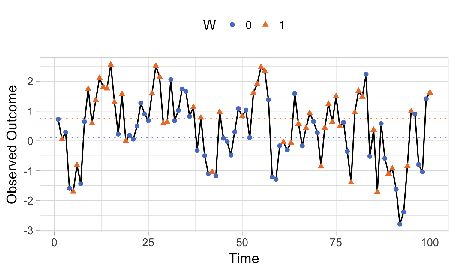
Observed outcomes: $Y_{t}^{\text{obs}}$

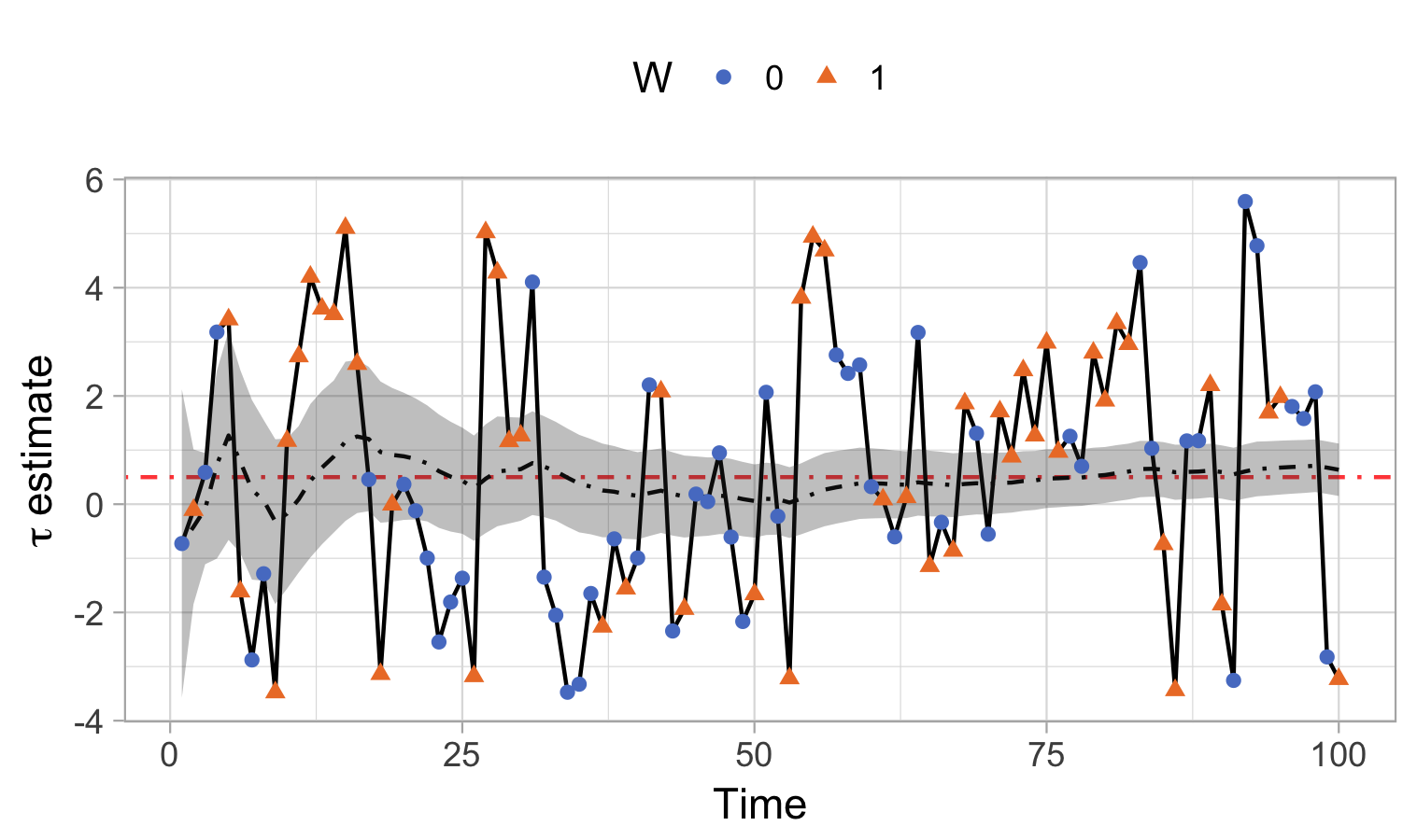
Estimates $\hat{\tau}_{t,0}$ and $\hat{\overline{\tau}}_{t}$ and estimand ${\overline{\tau}}$

Figure 2: Left: $Y_{1:T}^{\text{obs}}$ from a potential autoregression with $\mu_{1}=0.5$, $\mu_{0}=0$, $\phi=0.5$, $\sigma_{1}=\sigma_{0}=1$, the color indicate the received treatment and the dotted lines are the observed average. Right: the estimate of $\hat{\tau}_{t,0}$ at each point, the black dotted line is the running average of the estimates, the gray polygon is the corresponding 95% confidence interval and the red dotted line is the true value of $\bar{\tau}_{0}$.

Figure 2 (right), shows $\widehat{\tau}_{t,0}$ plotted against time.  Also plotted is the sequential average of these differences and a 95% confidence interval.  The plotted orange line, which again indicates $\overline{\tau}_{0}$, is close to $\widehat{\overline{\tau}}_{0}$.

8.2 Simulation results

We study the sampling performance of our testing procedures using a potential autoregression with $\mu_{w_{1:t}}=\mu_{w_{t}}$, $\sigma_{w_{1:t}}=\sigma_{w_{t}}$, $\phi=0.5$, $\sigma_{1}=\sigma_{0}=1$ and

$$\text{Null}\text{: }\mu_{1}=\mu_{0}=0,\quad\text{Alternative}\text{: }\mu_{1}=0.2,\quad\mu_{0}=0.$$ (16)

We look at where $\varepsilon_{t}\overset{iid}{\sim}N(0,1)$ and $\varepsilon_{t}\overset{iid}{\sim}$ Cauchy.  The latter produces heavy tailed data.

8.2.1 Fixing the potential outcomes

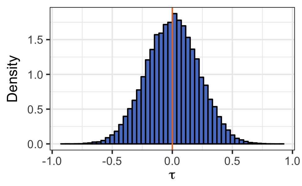
$\widehat{\bar{\tau}}_{1}$

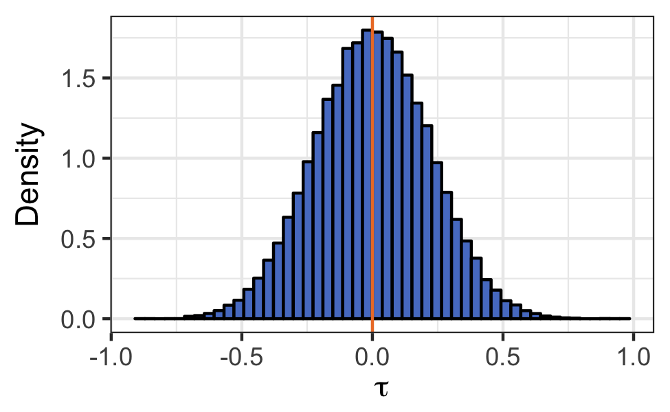
$\widehat{\bar{\tau}}_{2}$

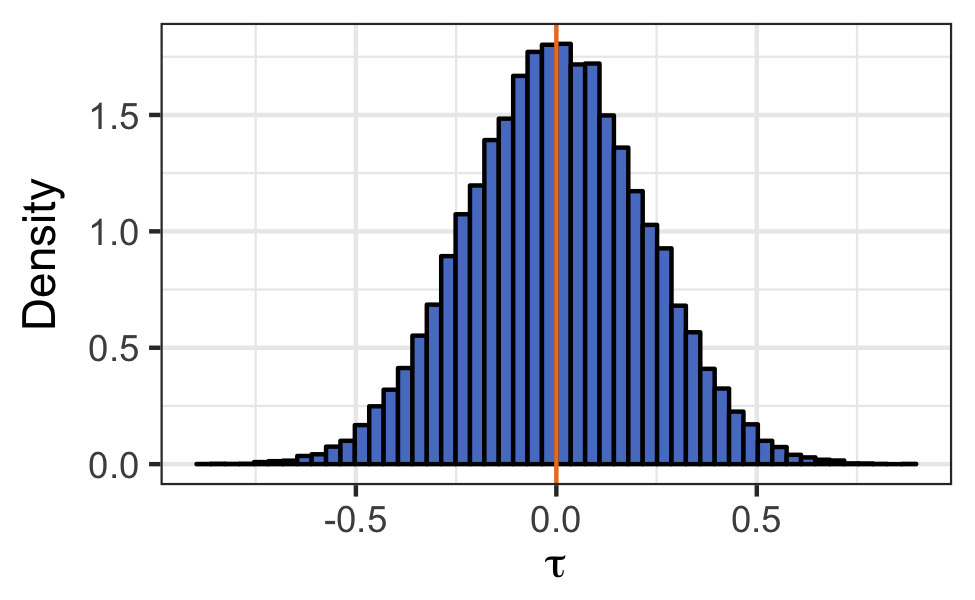
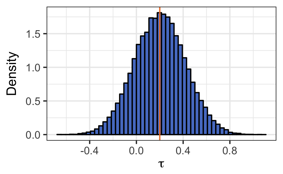
$\mu_{1}=0.2$, $\mu_{0}=0.0$

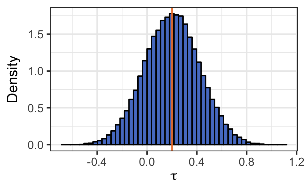
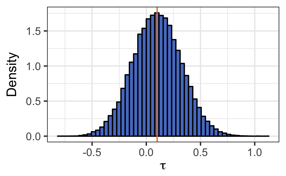
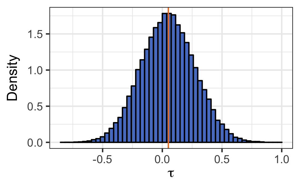
Figure 9: Histograms of different estimates obtain from 50,000 treatment paths for the same $Y_{1:T}$ with $T=100$ & $\phi=0.5$ where the treatment effect is either $\mu_{1}=0$ (top) or $\mu_{1}=0.2$ and the stocks are Gaussian. The 1st column is from the $\widehat{\bar{\tau}}_{0}$ estimator, the 2nd column is the $\widehat{\bar{\tau}}_{0}^{(1)}$ estimator, the 3rd column is the $\widehat{\bar{\tau}}_{1}$ estimator & the 4th column is the $\widehat{\bar{\tau}}_{2}$ estimator. All of the estimators have similar variance, & are centered at the true data generating value.

To illustrate the central limit approximation we first generate the potential outcomes and then, fixing $Y_{1:T}(\bullet)$, simulate over different $W_{1:T}$. Figure 3 shows our results for the randomization distribution of $\widehat{\overline{\tau}}_{0}$ given in (6). When $\varepsilon_{t}\overset{iid}{\sim}N(0,1)$ the estimates obtained from different treatment paths quickly converge to a normal distribution. When $\varepsilon_{t}\overset{iid}{\sim}$ Cauchy a longer experimental time is require to reach approximate normality. This is due to the heavy tails of the noise. Figure 9, in the web appendix, shows examples of $\widehat{\overline{\tau}}_{1}$, $\widehat{\overline{\tau}}_{0}^{(1)}$ and $\widehat{\overline{\tau}}_{1}^{(1)}$ also appear roughly Gaussian for $T=100$, for different values of $\mu_{t}$.

$\widehat{\bar{\tau}}_{0}$

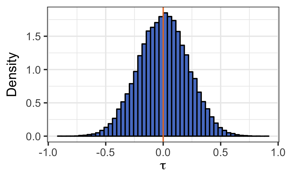
$\widehat{\bar{\tau}}_{0}$

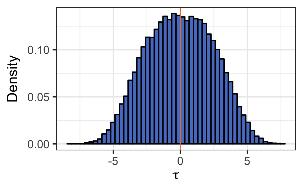
$\widehat{\bar{\tau}}_{0}$

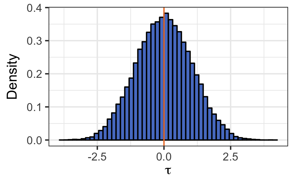
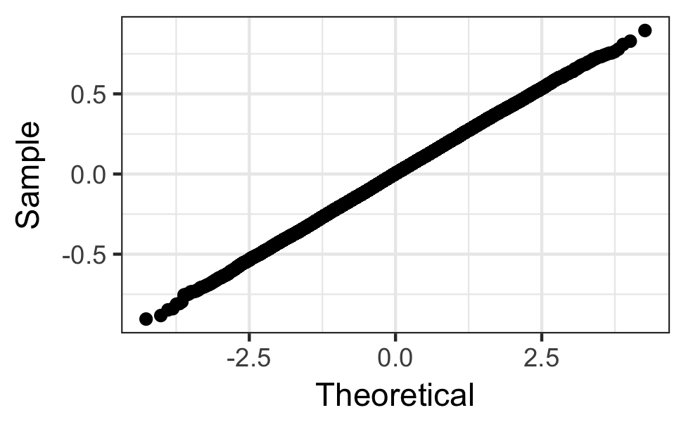
$N(0,1),T=100$

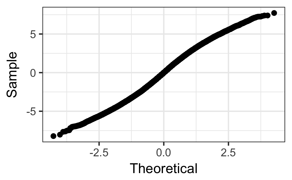
Cauchy, $T=1,000$

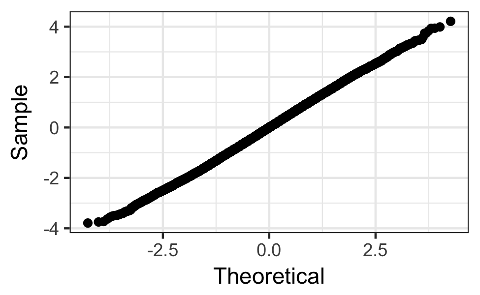
Cauchy, $T=10,000$

Figure 3: Sampling behavor of estimators.  Top: histograms of $\widehat{\bar{\tau}}_{0}$ over $W_{1:T}|Y_{1:T}(\bullet)$ based on conditioning on a single draw from $Y_{1:T}(\bullet)$, i.e. fixing the potential outcomes. Bottom: Q–Q normal plot. For heavy tailed distributions a larger sample is need to achieve asymptotic normality. The vertical orange line represents the true value of the estimand.

8.2.2 Replicating over potential outcomes

We also need to evaluate the frequentist properties over the sampling distribution – explicitly averaging over the potential outcomes using the potential autoregression. To this end, we generated 50,000 independent copies of $Y_{1:T}$, under the null assumption of no treatment effect, and computed the randomization based $p$-value distribution for $\widehat{\overline{\tau}}_{0}$.  For each replication the tests are exact, and the $p$-values follows a discrete uniform distribution.  Of more interest is that we also applied the conservative test which relies on the approximate normality of $\widehat{\overline{\tau}}_{0}$.

The left hand side of Figure 4 shows the $p$-value distributions for $T=100$ in the conservative test cases.  We omit the results for the exact unstandardized test.  The $p$-values obtained from the conservative tests and the randomization test show similar patterns, but the conservative test has slight lower $\alpha$ level due to the overestimation of the variance. Figure 4 also shows the relative power of the two methods as the treatment effect increases for $\widehat{\overline{\tau}}_{0}$, holding all other factors fixed.  Notice how the conservative test is only slightly less powerful than the randomization based test. The second figure shows the relative power of the two methods as a function of the $\phi$ parameter for the 1 lag case.

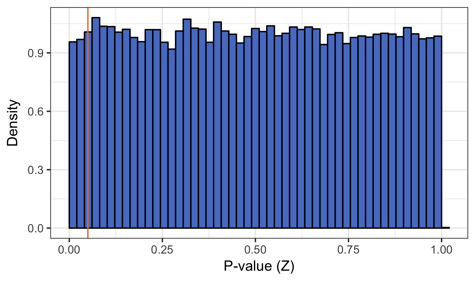
Conservative test: $\widehat{\bar{\tau}}_{0}$

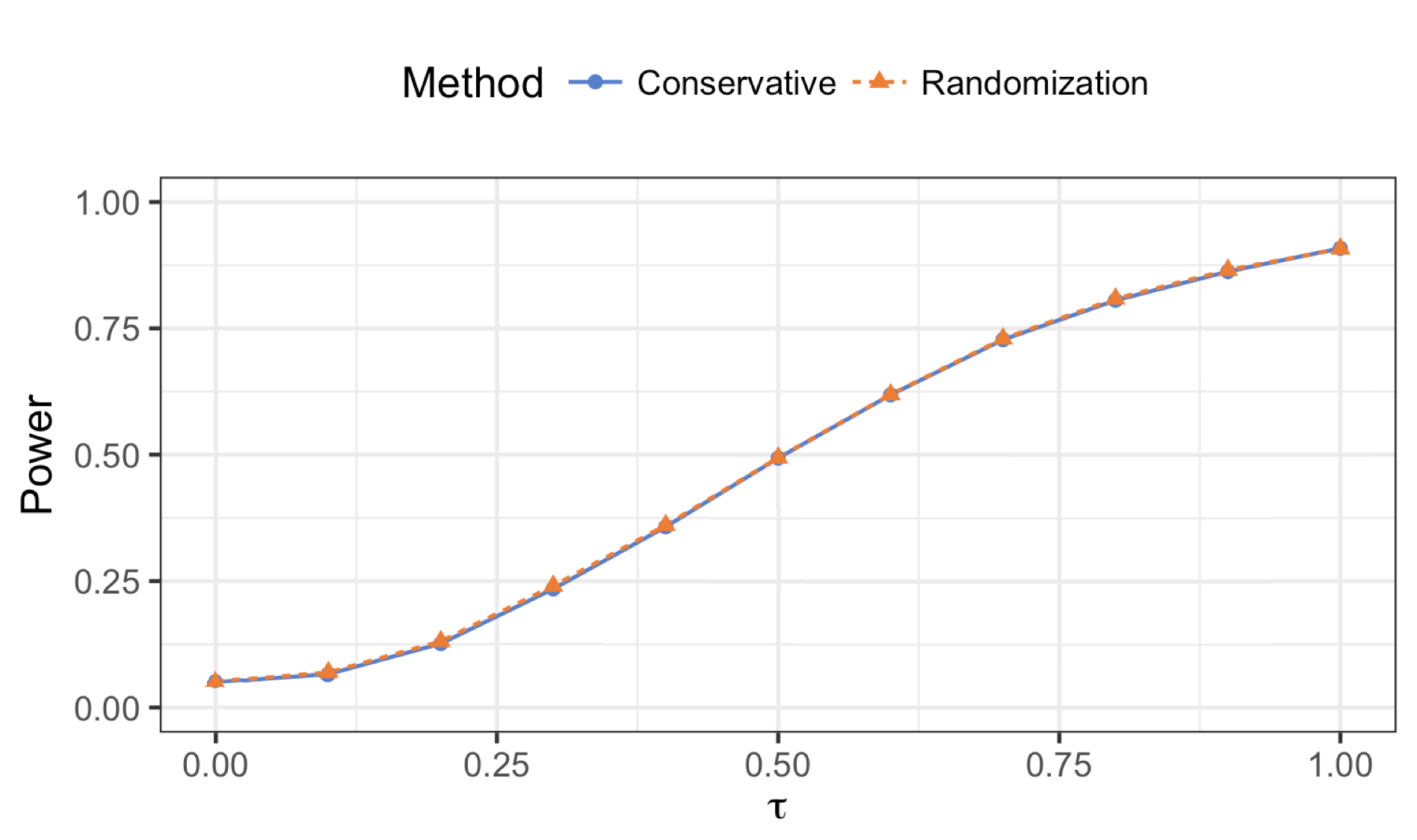
For $\widehat{\bar{\tau}}_{0}$ as $\bar{\tau}_{0}$ varies

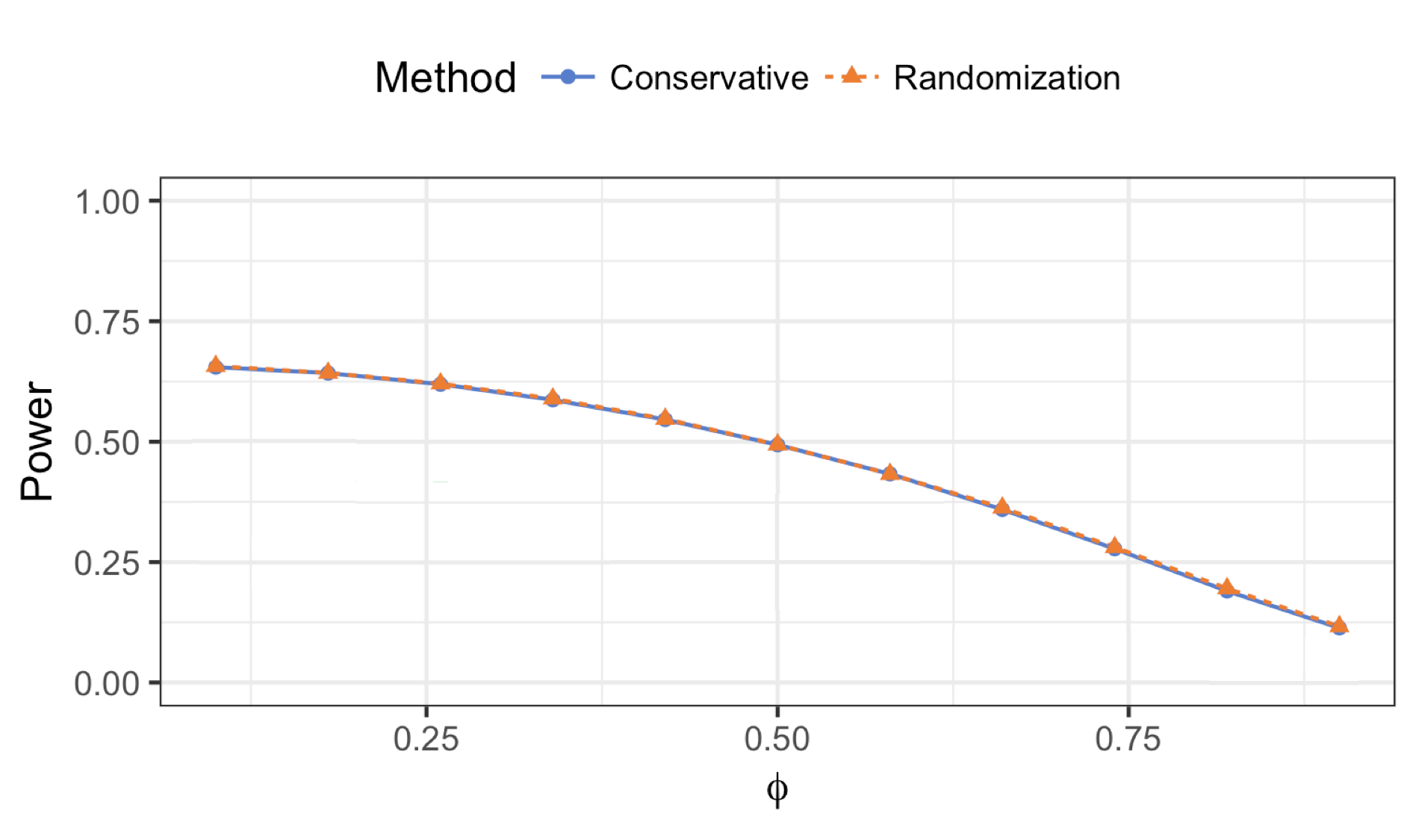
For $\widehat{\bar{\tau}}_{1}$ as $\phi$ varies

Figure 4: Left: distributions of $p$-values over $50,000$ simulations for $T=100$ when there is no treatment effect, using the conservative test using the normal approximation. The orange line represents the $0.05$ cut off. Middle and right: The relative power for the tests as $\tau$ increases for fixed $\phi=0.5$ (middle) and as the $\phi$ parameter increases for fixed $\tau=0.5$ (right). The conservative test performs only slightly worse that the exact randomization test. The noise distribution is $N(0,1)$.

8.3 Pooled estimation: averaging over multiple units

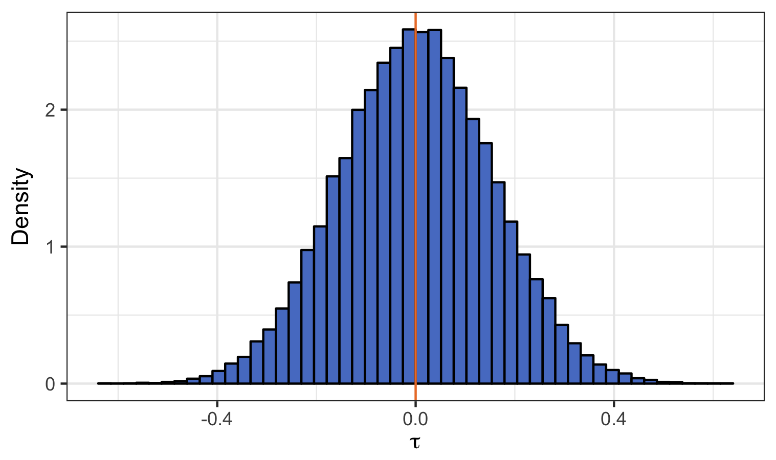
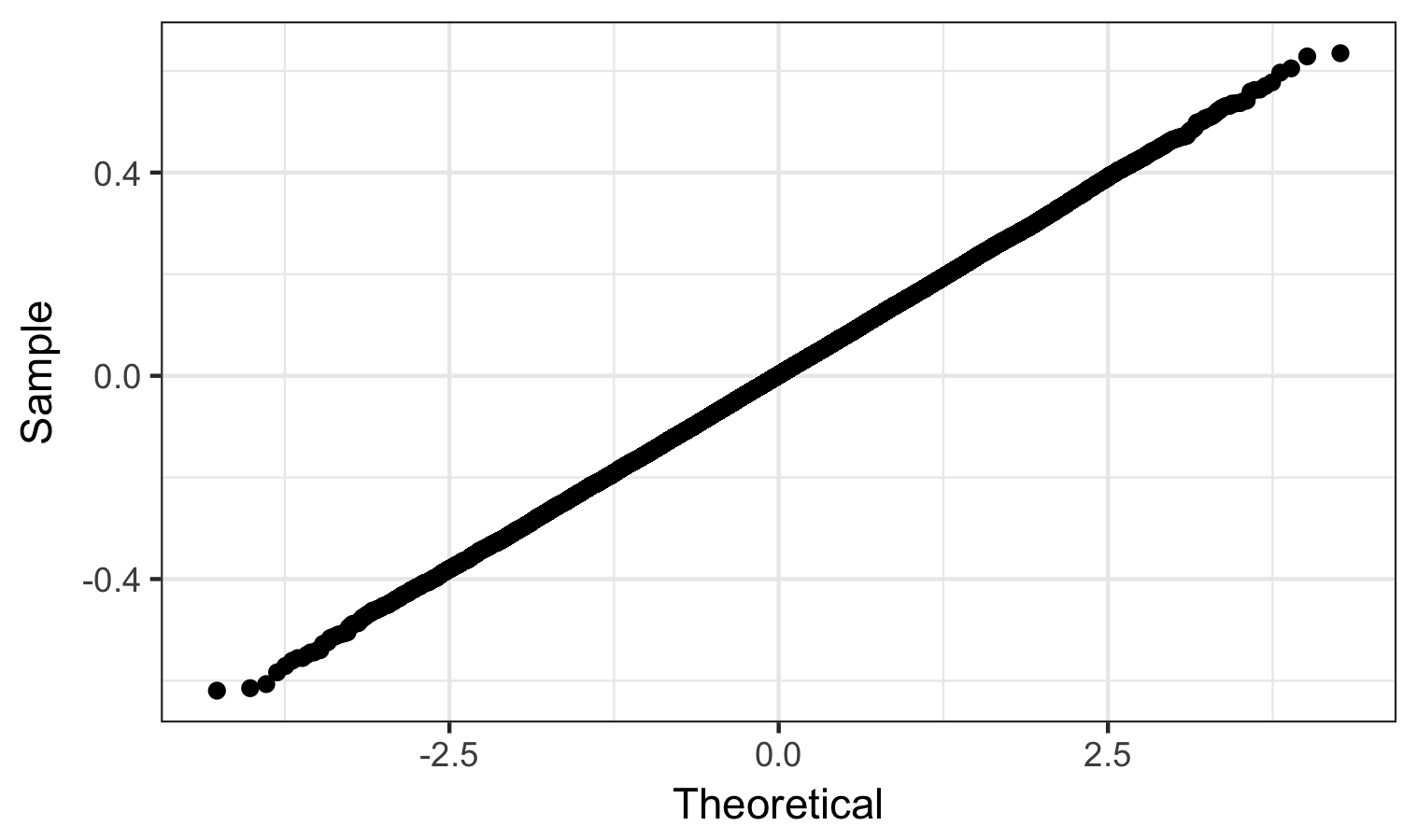
Figure 10: The distribution of the pooled estimator of $\bar{\tau}$ over 50,000 simulations, for $n=2$ experiments and $T=100$. Notice how the variance is smaller than the unpooled version in Figure 9.

To investigated the behavior of the pooled estimator, we generated two independent experiments for $T_{1}=T_{2}=100$ and combined them, as described in (14). Figure 10, in the web appendix, shows how the distribution of the pooled estimator is well approximated using the CLT.  The variance of the pooled estimator is lower than that obtained from each of the individual experiments.

9 Empirical example from finance

9.1 Trading futures contracts

Here we analyze experiments carried out by AHL Partners, a quantitative trading group that mainly trades in financial futures. Within each futures market their desired positions are decided solely by algorithms and currently available financial data. Once their target position changes, they need to carry out “an order” within a prescribe time period e.g. buy $20 million of gold futures over the next trading day. These orders are often large, and they make such orders frequently, so trading well is vital to their performance as a group.

The firm has two ways of executing an order, either using a human trader or an algorithm. Both methods typically avoid executing the whole order in one go as this could deliver a poor execution price. Instead, they break up the order into smaller pieces and make a sequence of trades to “fill” the order. As they trade the price will often move against them, i.e. rise if they are executing a series of buys, or fall if they are carrying out a series of sells.  However, these rises and falls are somewhat masked by the general volatility in the market as filling the order takes time.

This group allocates the subset of orders which have order size between a fixed lower and upper bound (these bounds are time invariant in the experiments covered by our data, but differ over the markets.  For confidentiality reasons we are unable to reveal these bounds), to humans traders and algorithmic traders randomly, to experimentally work out which is more effective at trading their orders. The treatments were always i.i.d. Bernoulli, ignoring past data.  Hence this setup obeys our non-anticipating treatments assumption.

					Median per Order
	Prob of Treatment		Numbers of orders		Number of trades		Execution time
	$<$July 12	$>=$ July 12					(in minutes)
Market			A	B	A	B	A	B
1	0.50	0.25	147	105	62	132	29.7	6.6
2	0.50	0.50	85	64	123	118	34.6	13.3
3	0.50	0.25	281	95	109	108	44.1	14.3
4	0.50	0.50	36	42	102	71	21.9	8.0
5	0.25	0.25	81	22	118	103	40.9	10.9
6	0.50	0.50	39	41	19	5	34.6	4.4
7	0.50	0.50	118	129	82	71	28.9	5.0
8	0.50	0.50	71	72	38	28	24.2	7.7
9	0.50	0.50	178	239	26	15	19.6	0.6
10	0.50	0.25	272	154	62	27	44.7	4.4

Table 1: Summary information for the ten different markets in 2016, with method A being control ($W_{t}=0$) and B being treatment ($W_{t}=1$). The number of orders is the number of experiments conducted in 2016 in each market. In three markets the probability of treatment was changed on midnight 12 July 2016.  

AHL Partners provided us with 10 sets of data from 2016; all are from trading index equity futures markets, where the underlying indices are from the US, Europe, and Asia. We will regard each of these 10 markets as separate units.

Table 1 provides the number of trades in each market during 2016, the median number of trades per order and the median number of minutes it takes to execute the order.  In both cases the numbers are broken down into the two trading methods.  To protect their confidential information they did not tell us which of methods “A” and “B” correspond to a human trader or algorithmic trader nor the identity of the individual markets.  Throughout we label method “A” as Control ($W_{t}=0$) and method “B” as Treatment ($W_{t}=1$).

Table 1 shows that method “A” typically trades more often when filling an order, but this varies over the market. “A” generally fills the order roughly three times slower than method “B”.  The group changed on midnight 12th July 2016 the probability of allocating to the treatment, method “B”, in three of the markets.  This is detailed in the Table.

9.2 Definition of financial slippage

The quality of each order’s execution is measured by “slippage,” which is a simple function of the trade prices and volumes at which the order was executed.  Slippage will be the “outcome” $Y_{t}^{\text{obs}}$ from these financial experiments.  The traders would like $Y_{t}^{\text{obs}}$ to be as low as possible (minimizing trading costs).  It will be measured using a signed volume weighted average price (VWAP) minus the mid-price scaled by mid-price (e.g. Berkowitz et al. (1988) and Calvori et al. (2013)).  The details are in the Web Appendix B.5.

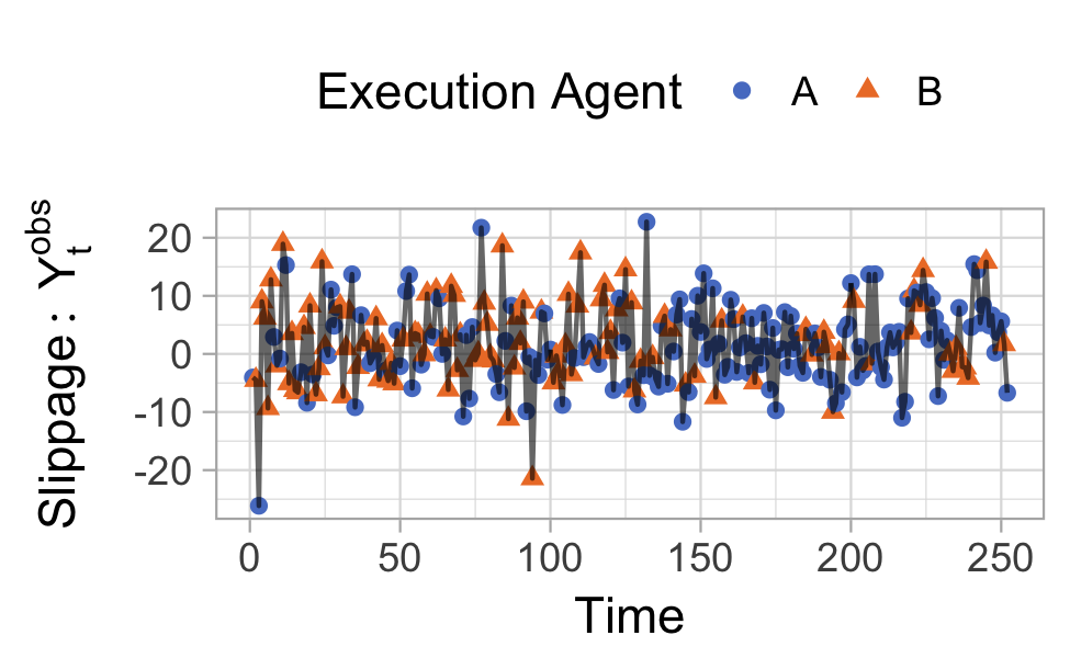
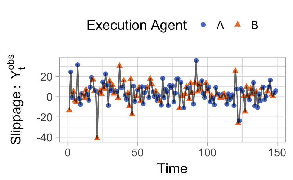
Figure 5: Left: The total slippage $Y_{t}^{\text{obs}}$ per order for Market 1. Orange indicates method “A” and blue “B”. Right: The total slippage $Y_{t}^{\text{obs}}$ per order for Market 2.

From these experiments we will use the time series of slippages $Y_{t}^{\text{obs}}$ as our primary outcome of interest, and the treatment $w_{t}^{obs}$ which will be 0 (the control) if method “A” is used to trade and a 1 (the treatment) if method “B” is used. The right plot of Figure 5 shows an example of the primary outcome for Markets 1 and 2, the remaining eight are given in the web appendix.

Taking a step back, modelling the dynamics of asset price returns is challenging as returns are very thick tailed and exhibit long-range volatility clustering (e.g. Taylor (2005)).  Our approach, which just uses the randomization of the experiment, does not need to make a stand on modelling the dynamics of returns and hence is entirely objective.

9.3 Inference on $\widehat{\bar{\tau}}_{p}$

Table 2 shows the average slippage of A and B as well as the estimated $\widehat{\bar{\tau}}_{0}$, $\widehat{\bar{\tau}}_{1}$ and $\widehat{\bar{\tau}}_{2}$ and the corresponding $p$-values.

Market	Average Slippage		$\widehat{\overline{\tau}}_{0}$	p.val	$\widehat{\overline{\tau}}_{1}$	p.val	$\widehat{\overline{\tau}}_{2}$	p.val
	A	B
1	1.48	2.29	0.52	0.628	-0.78	0.382	-0.04	0.963
2	4.11	3.35	-1.80	0.315	0.53	0.771	-1.86	0.300
3	-0.05	1.07	0.54	0.634	-0.26	0.813	0.30	0.762
4	3.38	3.23	0.36	0.900	2.10	0.450	3.11	0.283
5	0.57	0.63	-0.42	0.743	-0.76	0.369	-0.04	0.448
6	-1.48	3.72	5.26	0.008	-1.33	0.507	0.54	0.791
7	1.99	1.64	-0.19	0.881	-2.50	0.043	-3.34	0.009
8	-0.08	-0.07	0.01	0.996	-0.79	0.732	-3.71	0.112
9	-2.19	0.64	2.60	0.000	0.19	0.803	-0.44	0.567
10	0.80	2.10	0.57	0.603	0.58	0.514	0.24	0.770
Overall	0.55	1.60	1.11	0.010	-0.33	0.396	-0.49	0.161

Table 2: Randomization based inference results for $\widehat{\bar{\tau}}_{0}$ and $\widehat{\bar{\tau}}_{1}$, “B” is considered treatment and “A” is considered control. The $p$-values (p.val) were obtained using the randomization method. The overall statistics are the pooled statistics.

To calibrate $\widehat{\bar{\tau}}_{0}$ it may be helpful to recall that the current annual expenses for holding the Vanguard 500 Index Fund Admiral Shares (VFIAX) is five basis points.  From Table 2 the firm is suffering an average slippage rate in equity futures of very roughly 0 to 2 basis points.  Thus if the firm trades in and out of the market with, say, $10M once during the year it would be likely to pay less in transaction charges than it would in expenses for holding $10M in the Vanguard fund for the year.  However, if it trades more often its trading costs could exceed the Vanguard level of costs.  Of course, there may be compensating advantages of more frequent trading, but we do not study that topic here.    From the results for $\widehat{\bar{\tau}}_{0}$, we can see that in markets 6 and 9 “A” performed significantly better than “B”. There are no markets where there is evidence of out performance by method “B”.  The lagged versions, $\widehat{\bar{\tau}}_{1}$ and $\widehat{\bar{\tau}}_{2}$, suggest little lagged casual dependence, with only 1 out of 20 statistics being statistically significant, that at lagged 2 for market 7.

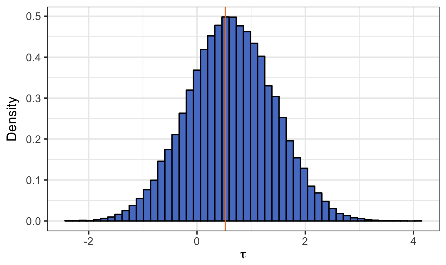
Market 1

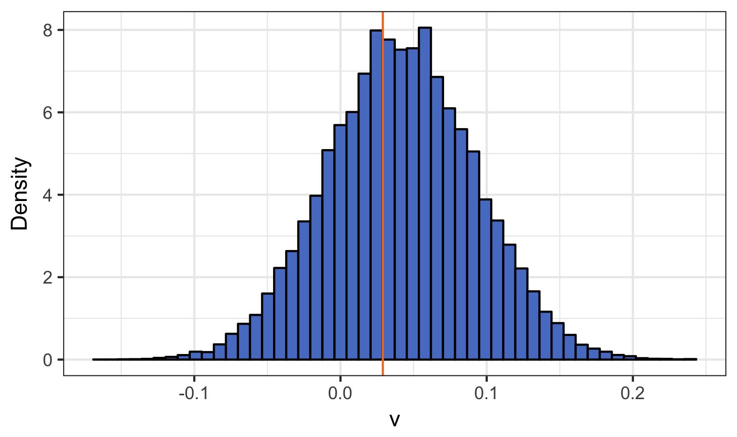
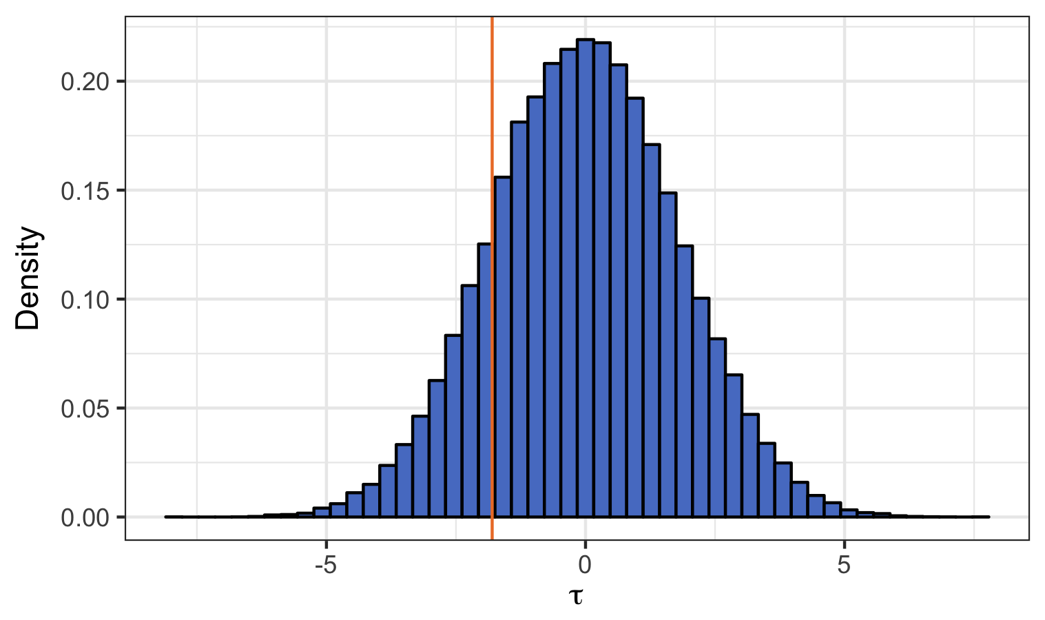
Market 2

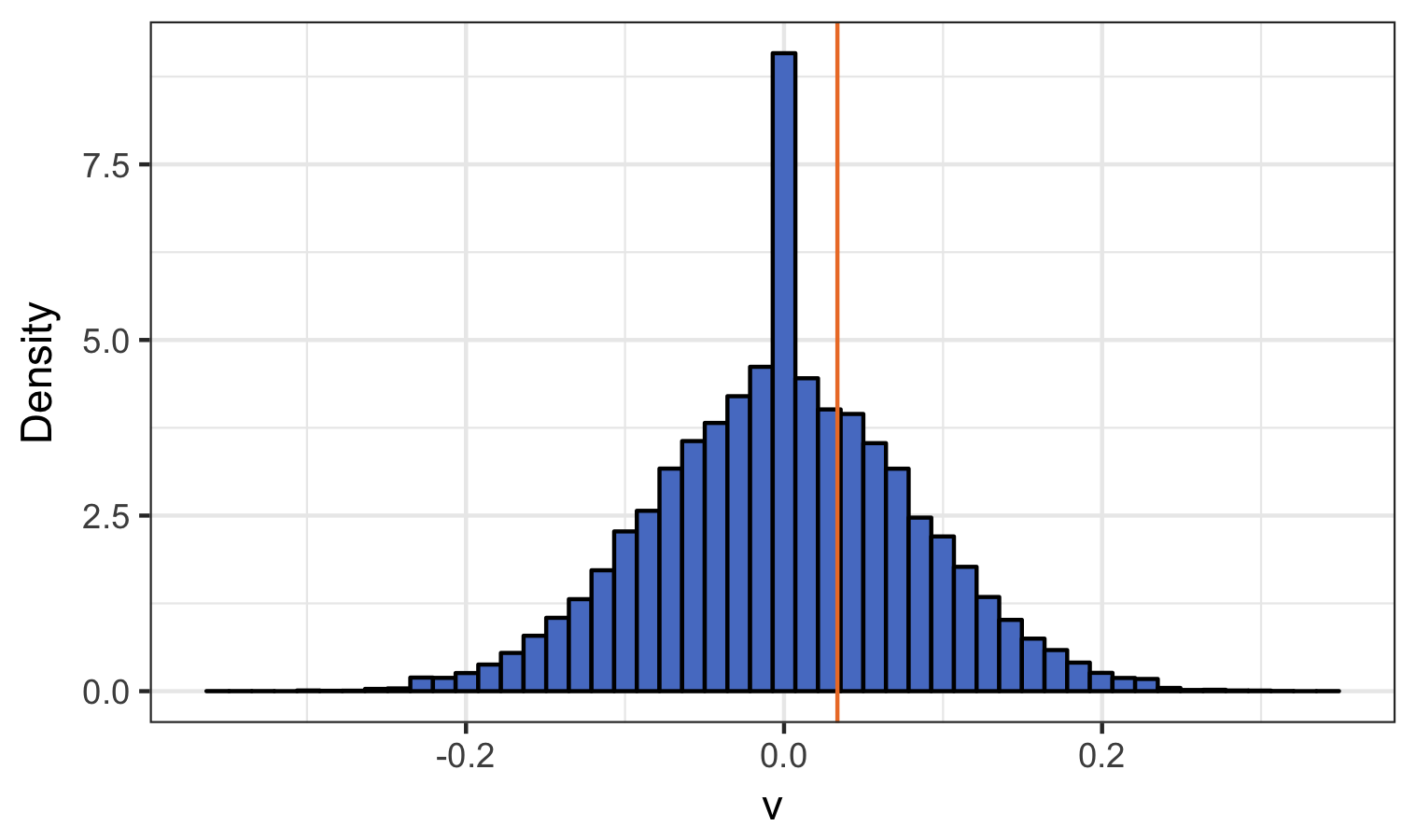
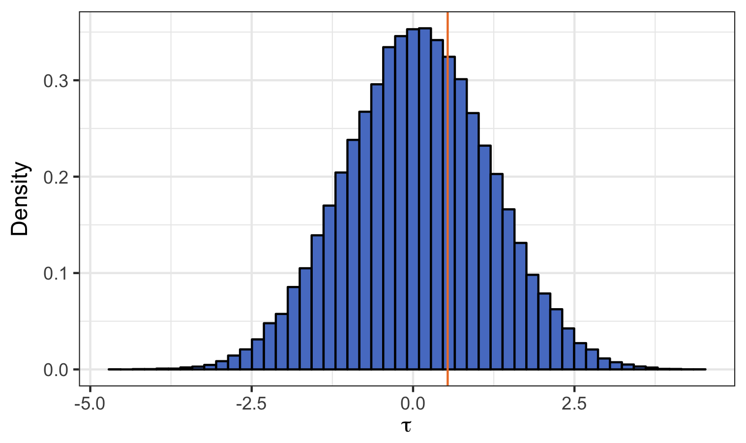
Market 3

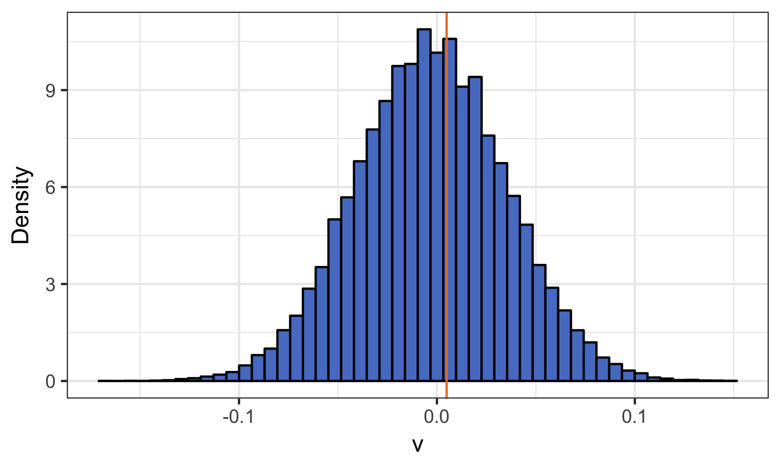
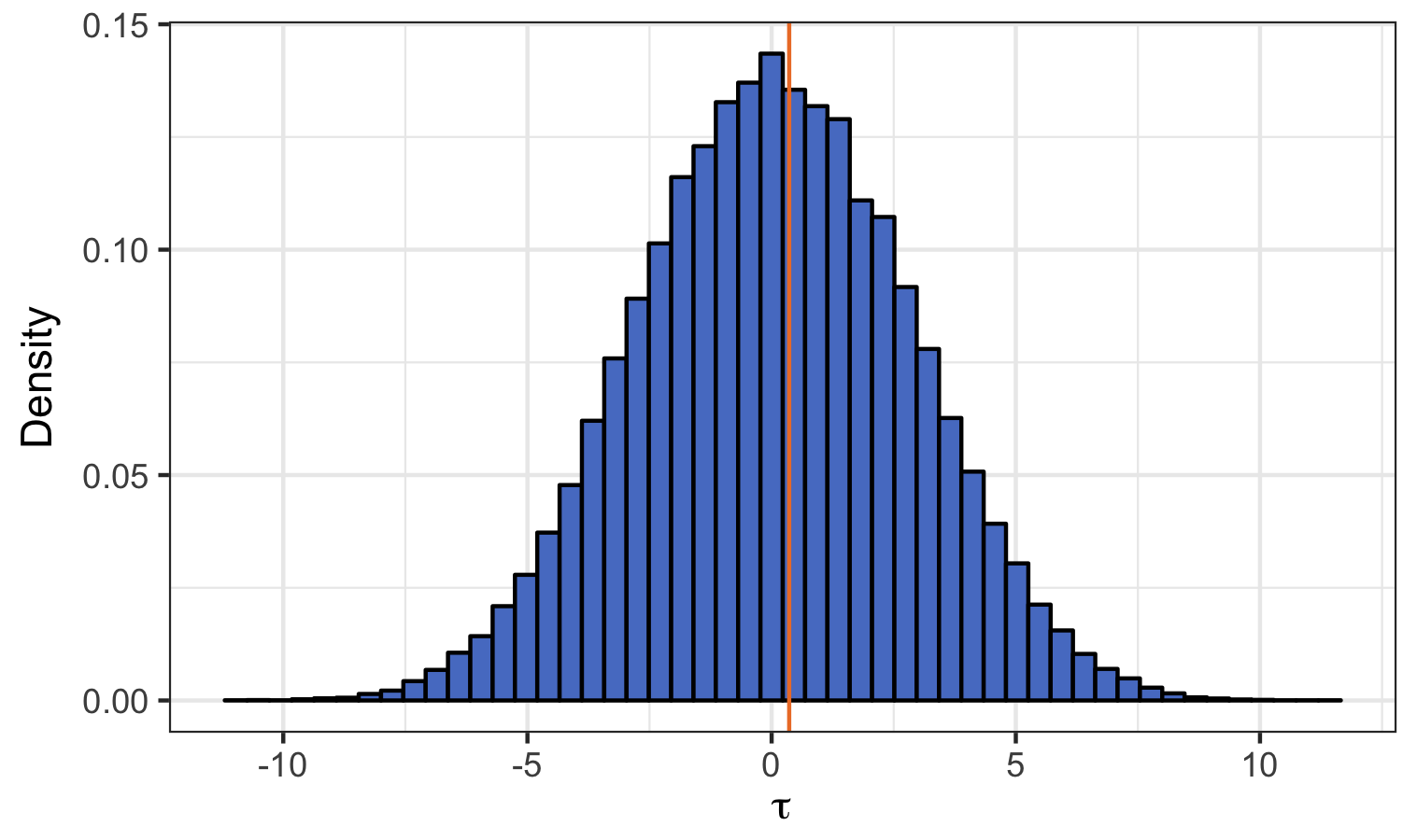
Market 4

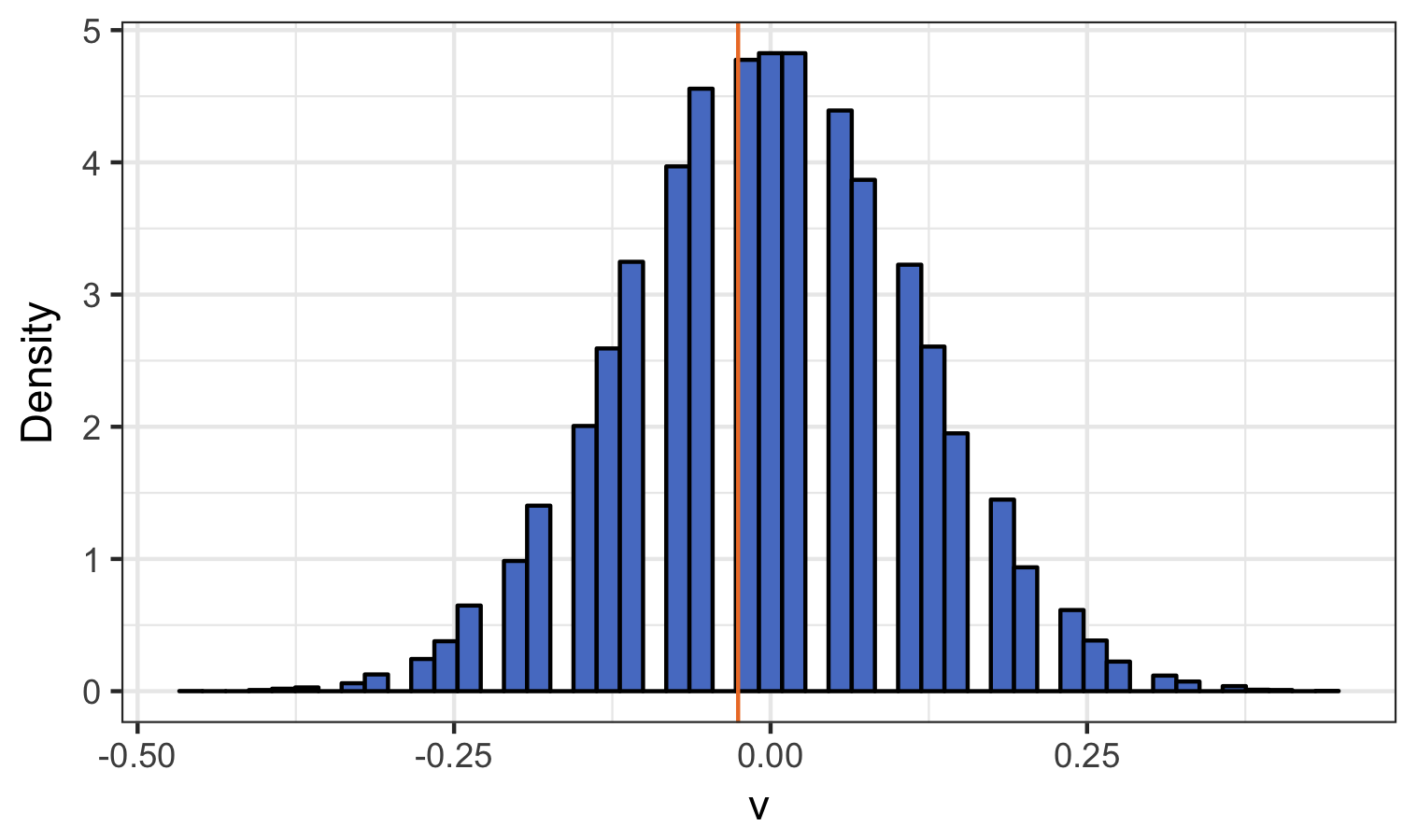
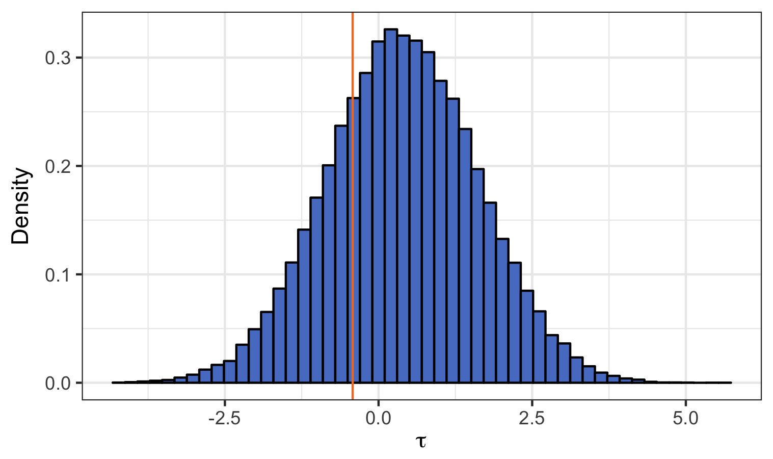
Market 5

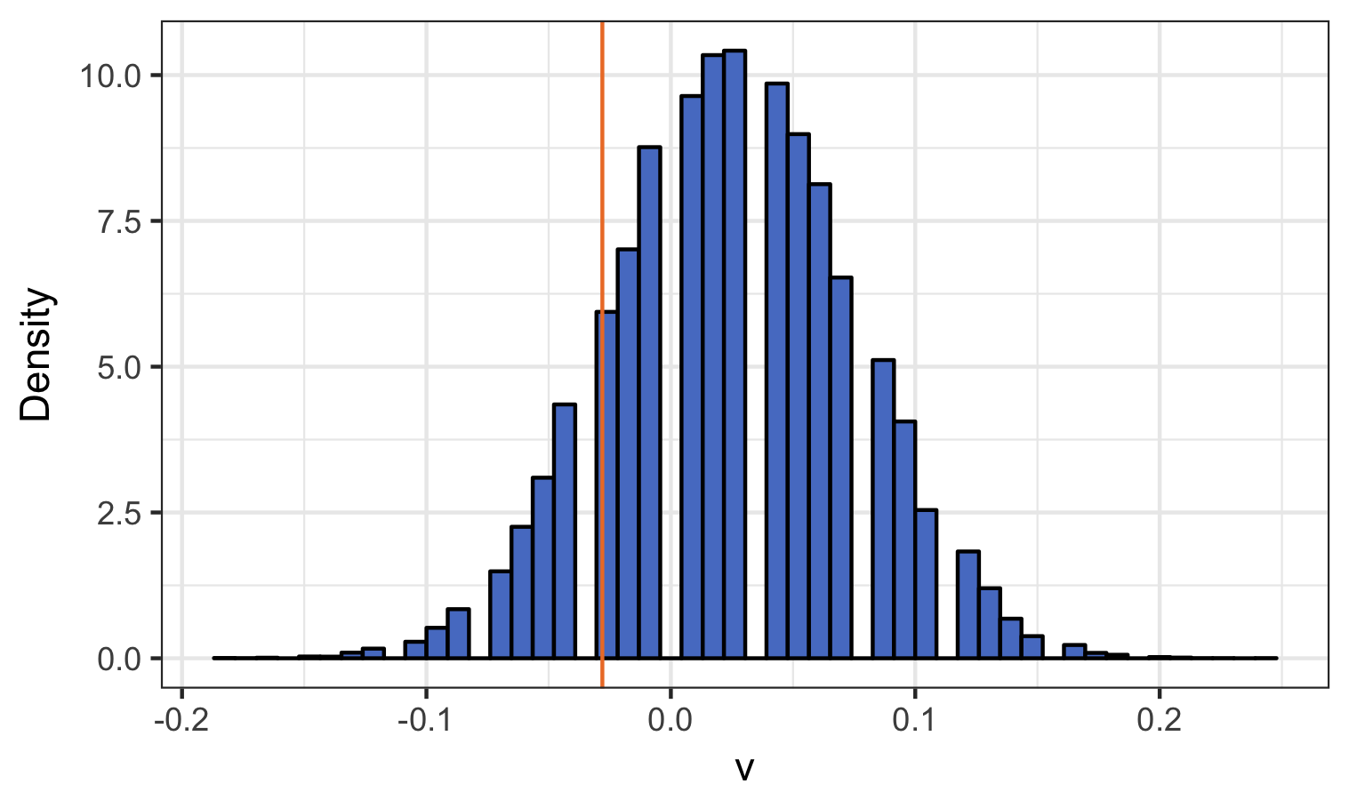
Market 7

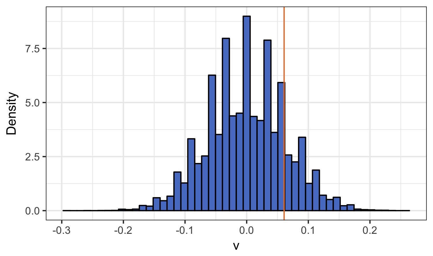
Market 8

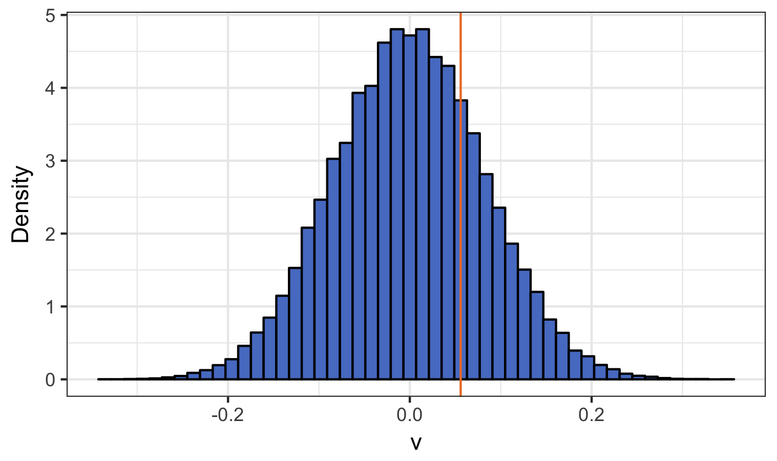
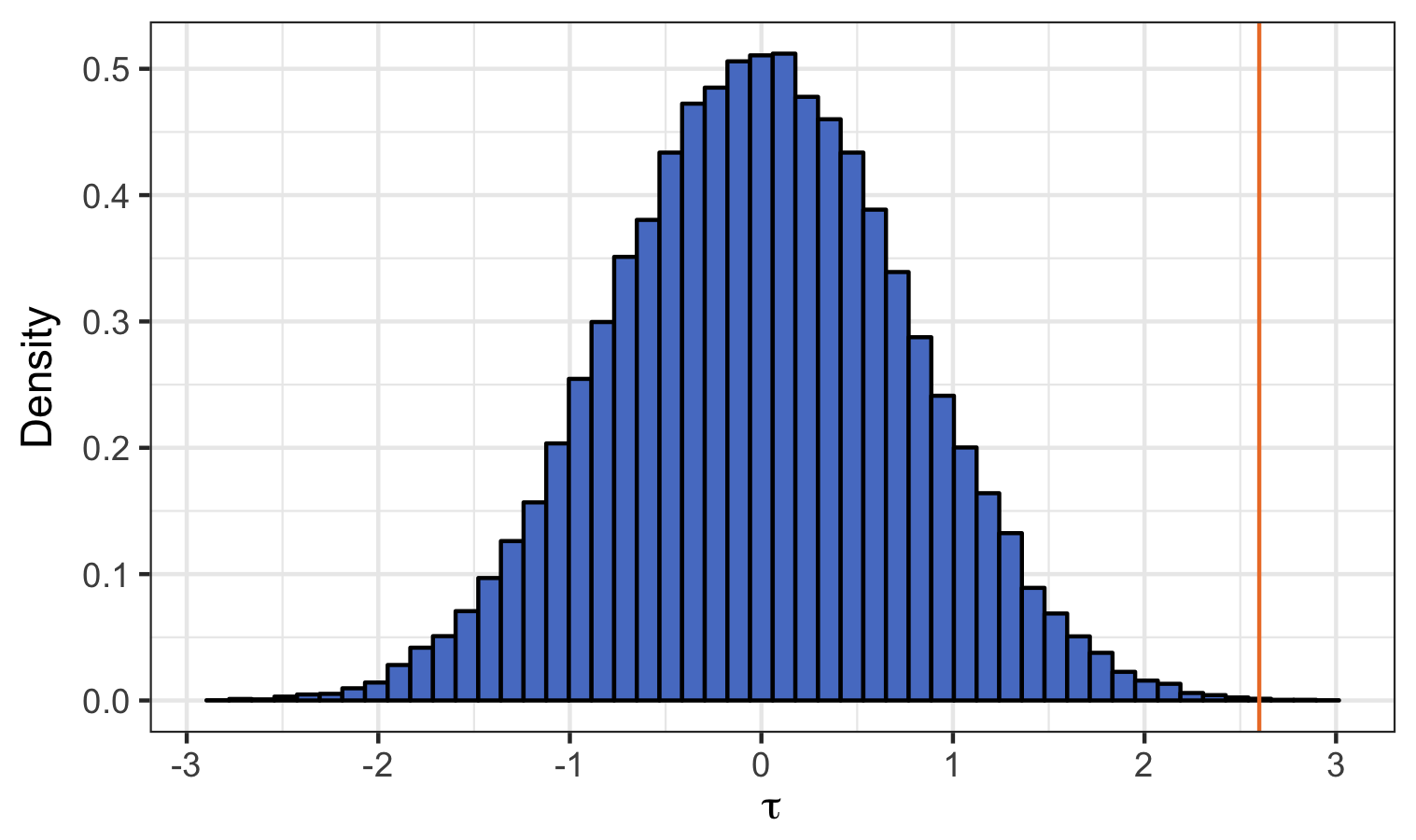
Market 9

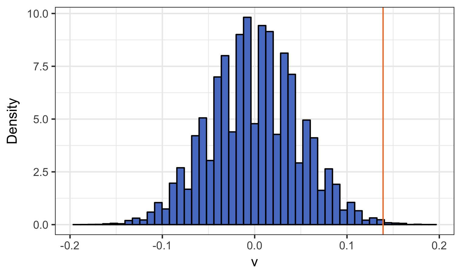
Figure 12: Randomization Distribution for Market 2 through 9, left using the $\widehat{\bar{\tau}}_{0}$, right using the $\widehat{\bar{v}}_{0}$. The orange line indicated the observed value of the statistic.

Figure 6 shows the randomization distribution of the statistic $\widehat{\bar{\tau}}_{0}$ for markets 6 and 10. The value of the observed statistic is shown by the vertical orange line.  The unstandardized statistic’s randomization distribution looks symmetric and smooth around 0.  Figure 12, in the web appendix, shows the results for the other markets.

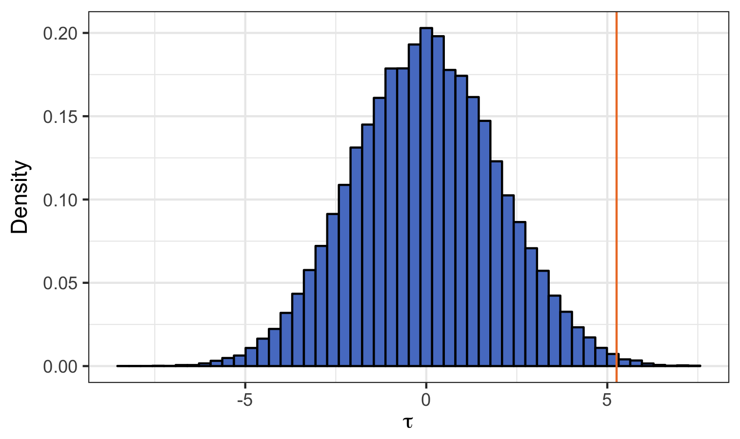
Market 6: $\widehat{\bar{\tau}}_{0}$

Market 10: $\widehat{\bar{\tau}}_{0}$

Figure 6: Randomization distribution for $\widehat{\bar{\tau}}_{0}$ Market 7 and 10. The vertical orange line indicated the observed value of the statistic $\widehat{\bar{\tau}}_{0}$.

9.4 Pooled estimation and lagged estimation

In Section 7, we explained how to jointly analyze the results for multiple units.  The treatments are i.i.d. Bernoulli, so continue to be independent of potential outcomes.

The most powerful procedure we proposed is the randomization based test.  When we applied it to all 10 markets we obtain a highly significant result, indicating that the slippage for method “A” is likely to be lower than that for method “B”.

The randomization distribution under the no temporal causal effects null (9) is shown in Figure 7, plotting the pooled $\widehat{\overline{\tau}}_{0}$ and $\widehat{\overline{\tau}}_{1}$ and step cases $\widehat{\overline{\tau}}_{0}^{(1)}$ and $\widehat{\overline{\tau}}_{1}^{(1)}$.  As usual the observed value is shown by the orange vertical line.  The observed value is in the extreme right hand tail of the distribution.  The contemporaneous results are strongly in favor of method A out performing method B in a causal sense across the 10 markets, with a $p$-value close to zero.  There seems to be almost no lagged effect.  For financial data this is not surprising as there is a modest amount of serial correlation in financial returns through time.  These results do not change for higher order stepped and lagged step causal effects.  More results along these lines are shown in Table 3.

	No temporal causal effects?				No average temporal causal effects?
$p$	$\widehat{\bar{\tau}}_{p}$	p.val	$\widehat{\bar{\tau}}_{p}^{(1)}$	p.val	$\widehat{\bar{\tau}}_{p}$	p.val	$\widehat{\bar{\tau}}_{p}^{(1)}$	p.val
0	1.108	0.010	1.101	0.005	0.941	0	0.936	0
1	-0.337	0.396	-0.272	0.455	-0.327	0.087	-0.264	0.189
2	-0.494	0.161	-0.414	0.212	-0.412	0.041	-0.368	0.053
3	-0.029	0.933	-0.018	0.953	-0.061	0.750	-0.032	0.853
4	-0.046	0.882	-0.068	0.801	-0.123	0.478	-0.093	0.539

Table 3: Results from pooled hypothesis tests for the 10 Markets for the $p\geq 0$ lagged causal effects. The no temporal causal effects refers to the Fisher style sharp null test.  The no average temporal causal effects refers to the Neyman style null implemented using the CLT.

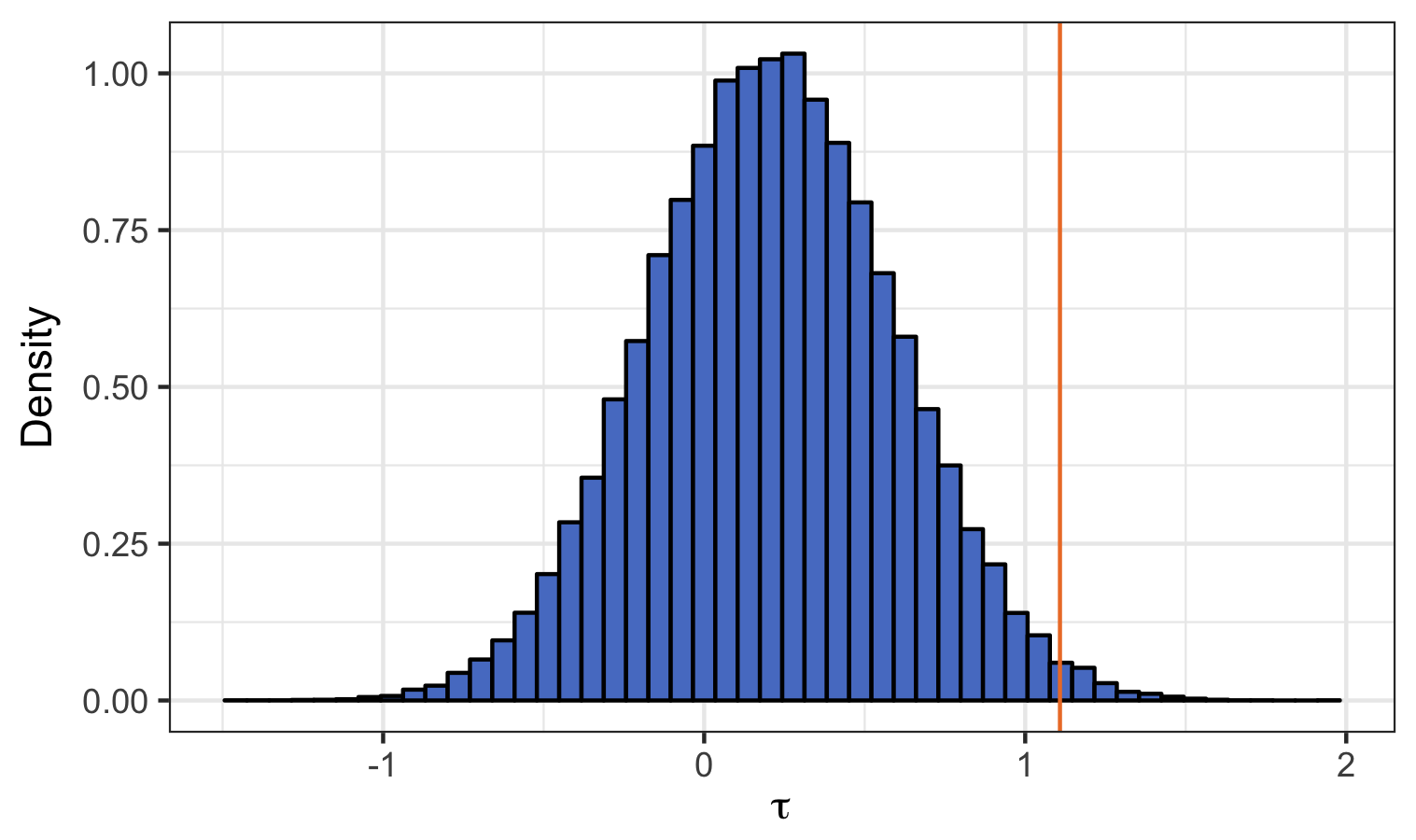
Pooled $\overline{\tau}_{0}$

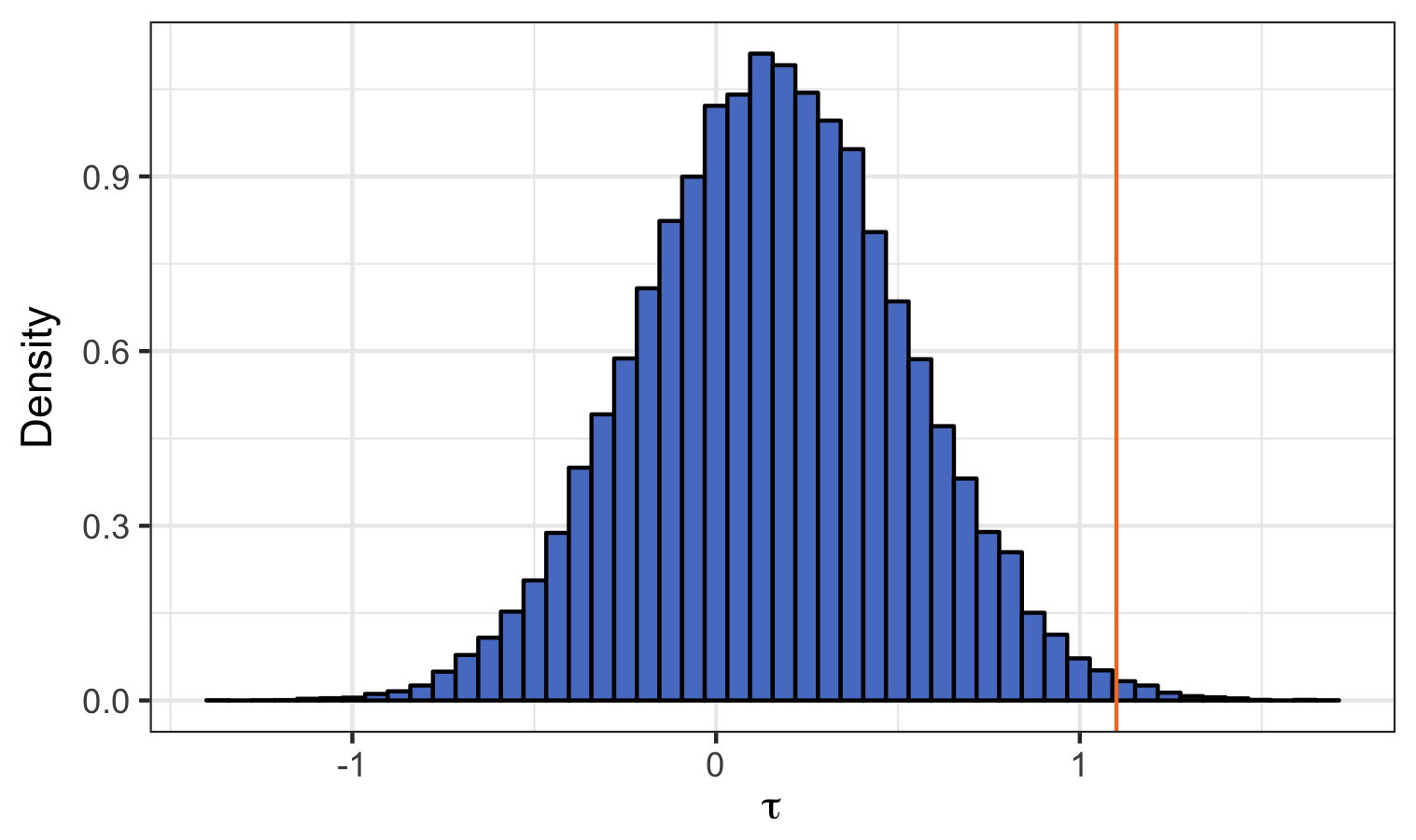
Pooled $\overline{\tau}_{0}^{(1)}$

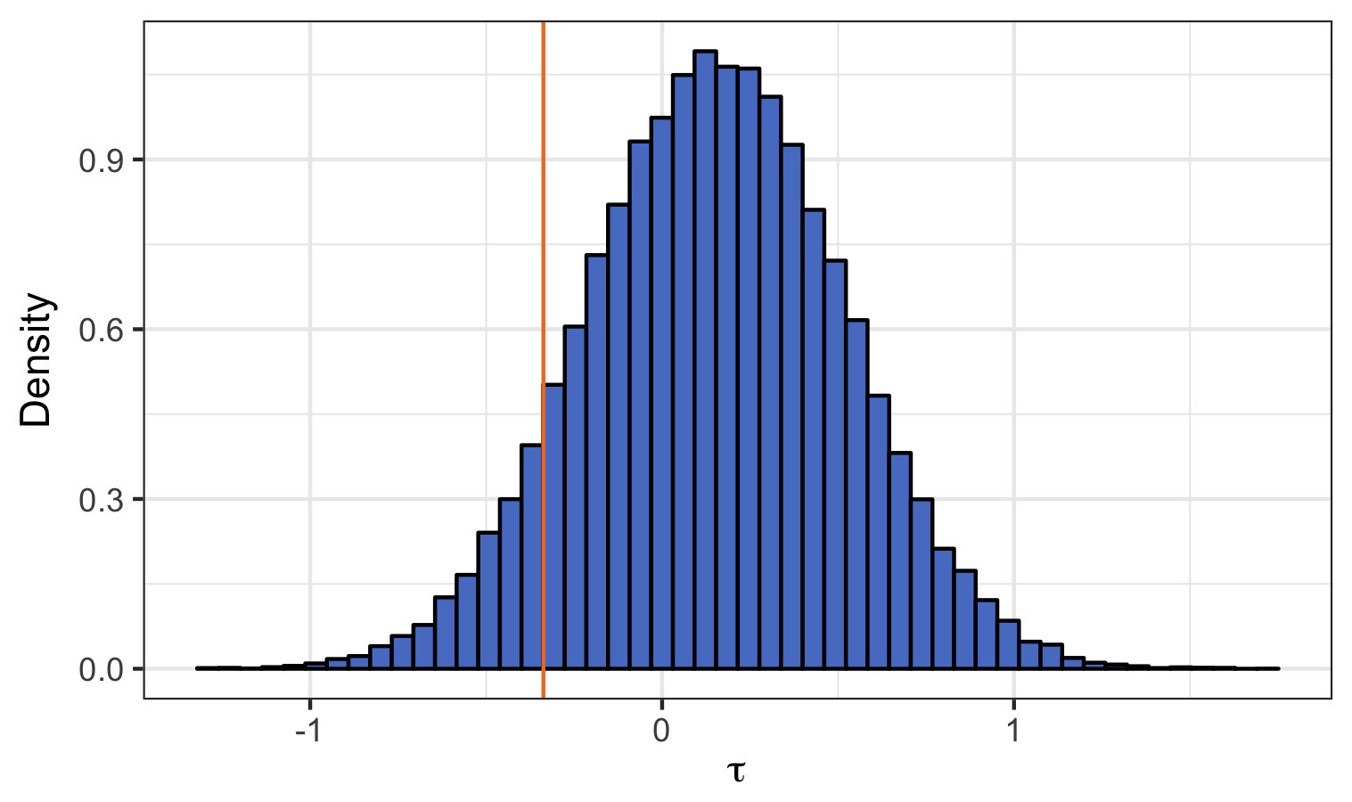
Pooled $\overline{\tau}_{1}$

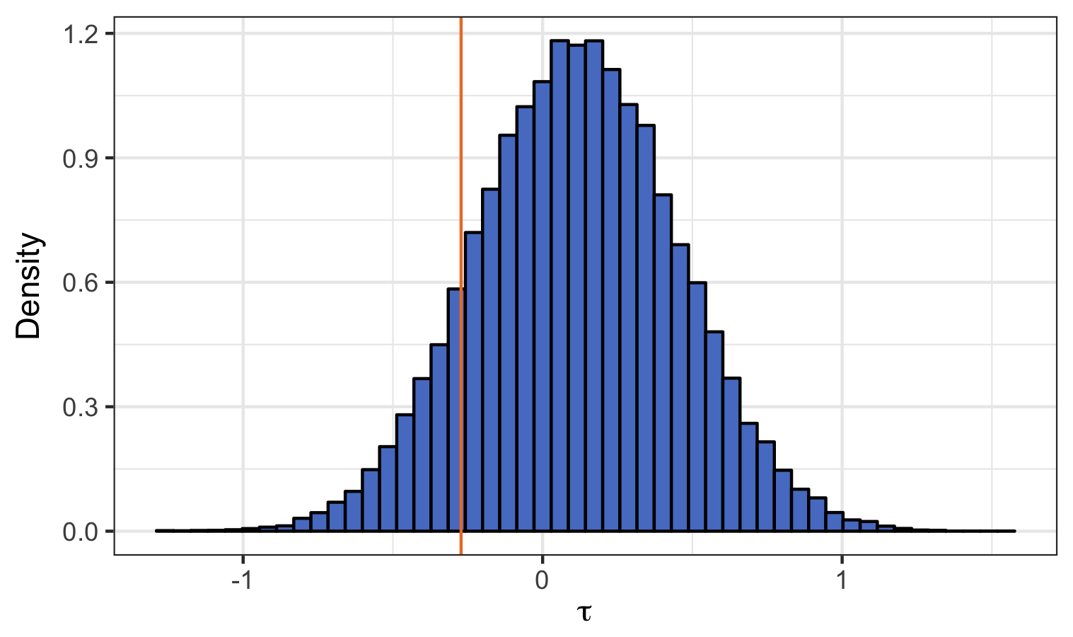
Pooled $\overline{\tau}_{1}^{(1)}$

Figure 7: Randomization distribution for the pooled statistics, using the $\overline{\tau}_{0}$ and $\overline{\tau}_{1}$ measures.  Both are also shown with 1 step. The vertical orange line indicated the observed value of the statistic. Notice that there is strong evidence indicated that there is a contemporaneous effect whereas there is little evidence indicated that there is a lagged effect.

10 Conclusion

In this paper, we use a potential outcome and treatment path framework to define causal estimands for experiments carried out on a single unit over time.  We define a broad class of estimands and proposed how to estimate them without any assumptions on the underlying potential outcomes.  Instead, we require that the treatments be non-anticipating and probabilistic.  We further propose two inferential strategies that utilize the probabilistic assignment of the treatment path.  Finally, we provide three strategies for generalizing our framework to multiple units.

Our first inferential procedure tests the sharp null of no temporal causal effect using the underlying randomization distribution.  These randomization based tests are exact and can be conducted using any of our proposed causal estimands.  Our second inferential procedure weakens the no temporal causal effect null hypothesis to the no average temporal causal effects null hypothesis.  Inference in this setting is conducted using a CLT and estimating an upper bound of the variance.

We apply our new methods on a large database of experiments carried out by a quantitative hedge fund, who decide to execute orders either using human traders or computers.  We show that one of these trading methods has a lower slippage rate than the alternative.

Appendix A Appendix

A.1 Proof of Theorem 1

For fixed $t$, we will further condense the adapted propensity score and use the notation $p_{1,w}=p_{t+p}(1,w)$, $p_{0,w}=p_{t+p}(0,w)$. For simplicity of exposition we use uniform weights, the extension to the non-uniform case is straightforward.  Then

$$\tau_{t+p,p}({1},{0}) = \frac{1}{2^{p}}\sum_{w\in\{0,1\}^{p}}Y_{t+p}(w_{1:t-1}^{\text{obs}},1,w)-Y_{t+p}(w_{1:t-1}^{\text{obs}},0,w)$$ (17)

$$\hat{\tau}_{t+p,p} = \frac{1}{2^{p}}\sum_{w\in\{0,1\}^{p}}\left\{\frac{1_{W_{t:t+p}=\left(1,w\right)}}{p_{1,w}}Y_{t+p}(w_{1:t-1}^{\text{obs}},1,w)-\frac{1_{W_{t:t+p}=\left(0,w\right)}}{p_{0,w}}Y_{t+p}(w_{1:t-1}^{\text{obs}},0,w)\right\}.$$

Hence $u_{t,p}=\hat{\tau}_{t+p,p}-\tau_{t+p,p}({1},{0})$ equals

$$\frac{1}{2^{p}}\sum_{w\in\{0,1\}^{p}}\left[\left\{\frac{1_{W_{t:t+p}=\left(1,w\right)}}{p_{1,w}}-1\right\}Y_{t+p}(w_{1:t-1}^{\text{obs}},1,w)-\left\{\frac{1_{W_{t:t+p}=\left(0,w\right)}}{p_{0,w}}-1\right\}Y_{t+p}(w_{1:t-1}^{\text{obs}},0,w)\right]$$

Now $\mathrm{E}(u_{t,p}|\mathcal{F}_{T,t-1})=0$, and $\mathrm{E}(\left|u_{t,p}\right|)<\infty$. Hence these errors are a martingale difference sequence and so uncorrelated through time.  The remaining issue is the variance.  Let,

$$R=\sum_{w\in\{0,1\}^{p}}\left\{c_{1,w}\left(1_{W=\left(1,w\right)}-p_{1,w}\right)-c_{0,w}\left(1_{W=\left(0,w\right)}-p_{0,w}\right)\right\},$$

where $c_{1,w}=Y_{t+p}(w_{1:t-1}^{\text{obs}},1,w)/p_{1,w}$, $c_{0,w}=Y_{t+p}(w_{1:t-1}^{\text{obs}},0,w)/p_{0,w}\$are known at $t-1$. Now

$$\mathrm{E}\left\{\left(1_{W=\left(1,w\right)}-p_{1,w}\right)\left(1_{W=\left(0,w^{\prime}\right)}-p_{0,w^{\prime}}\right)|\mathcal{F}_{T,t-1}\right\} = \mathrm{E}\left(1_{W=\left(1,w\right)}1_{W=\left(0,w^{\prime}\right)}|\mathcal{F}_{T,t-1}\right)-p_{1,w}p_{0,w^{\prime}}$$

$$= -p_{1,w}p_{0,w^{\prime}},$$

$$\mathrm{E}\left\{\left(1_{W=\left(j,w\right)}-p_{j,w}\right)\left(1_{W=\left(j,w^{\prime}\right)}-p_{j,w^{\prime}}\right)|\mathcal{F}_{T,t-1}\right\} = 1_{w=w^{\prime}}p_{j,w}-p_{j,w}p_{j,w^{\prime}}\quad\text{for }j=0,1.$$

So $\mathrm{Var}^{R}(R|\mathcal{F}_{T,t-1})$ equals

$$\sum_{w,w^{\prime}\in\{0,1\}^{p}}c_{1,w}c_{1,w^{\prime}}\left(1_{w=w^{\prime}}p_{1,w}-p_{1,w}p_{1,w^{\prime}}\right)+c_{0,w}c_{0,w^{\prime}}\left(1_{w=w^{\prime}}p_{0,w}-p_{0,w}p_{0,w^{\prime}}\right)$$

$$+\left(c_{1,w}c_{0,w^{\prime}}p_{1,w}p_{0,w^{\prime}}+c_{1,w^{\prime}}c_{w,0}p_{1,w^{\prime}}p_{0,w}\right)$$

$$= \sum_{w\in\{0,1\}^{p}}c_{1,w}^{2}p_{1,w}+c_{0,w}^{2}p_{0,w}+\sum_{w,w^{\prime}\in\{0,1\}^{p}}c_{1,w}c_{0,w^{\prime}}p_{1,w}p_{0,w^{\prime}}+c_{1,w^{\prime}}c_{0,w}p_{1,w^{\prime}}p_{0,w}$$

$$-c_{1,w}c_{1,w^{\prime}}p_{1,w}p_{1,w^{\prime}}-c_{0,w}c_{0,w^{\prime}}p_{0,w}p_{0,w^{\prime}}$$

$$= \sum_{w\in\{0,1\}^{p}}\left(\frac{Y_{t+p}(w_{1:t-1}^{\text{obs}},1,w)^{2}}{p_{1,w}}+\frac{Y_{t+p}(w_{1:t-1}^{\text{obs}},0,w)^{2}}{p_{0,w}}\right)$$

$$+\sum_{w,w^{\prime}\in\{0,1\}^{p}}Y_{t+p}(w_{1:t-1}^{\text{obs}},1,w)Y_{t+p}(w_{1:t-1}^{\text{obs}},0,w^{\prime})-Y_{t+p}(w_{1:t-1}^{\text{obs}},0,w)Y_{t+p}(w_{1:t-1}^{\text{obs}},0,w^{\prime})$$

$$+Y_{t+p}(w_{1:t-1}^{\text{obs}},1,w^{\prime})Y_{t+p}(w_{1:t-1}^{\text{obs}},0,w)-Y_{t+p}(w_{1:t-1}^{\text{obs}},1,w^{\prime})Y_{t+p}(w_{1:t-1}^{\text{obs}},1,w)$$

$$= \sum_{w\in\{0,1\}^{p}}\left(\frac{Y_{t+p}(w_{1:t-1}^{\text{obs}},1,w)^{2}}{p_{1,w}}+\frac{Y_{t+p}(w_{1:t-1}^{\text{obs}},0,w)^{2}}{p_{0,w}}\right)$$

$$-\sum_{w,w^{\prime}\in\{0,1\}^{p}}\left\{Y_{t+p}(w_{1:t-1}^{\text{obs}},1,w^{\prime})-Y_{t+p}(w_{1:t-1}^{\text{obs}},0,w^{\prime})\right\}\left\{Y_{t+p}(w_{1:t-1}^{\text{obs}},1,w)-Y_{t+p}(w_{1:t-1}^{\text{obs}},0,w)\right\}.$$

A.2 Proof of Lemma 1

Note that for any $w$ and $w^{\prime}$ we have the following bound, $\left\{Y_{t}(w)+Y_{t}(w^{\prime})\right\}^{2}=Y_{t}(w)^{2}+Y_{t}(w^{\prime})^{2}+2Y_{t}(w)Y_{t}(w^{\prime})$ is non-negative, so $Y_{t}(w)^{2}+Y_{t}(w^{\prime})^{2}\geq 2Y_{t}(w)Y_{t}(w^{\prime})$. By proof of Theorem 1 we can write $\mathrm{Var}^{R}(u_{t,p}|\mathcal{F}_{T,t-1})$, ignoring the scaling, in the following way,

$$\sum_{w\in\{0,1\}^{p}}\left(\frac{Y_{t+p}(w_{1:t-1}^{\text{obs}},1,w)^{2}}{p_{1,w}}+\frac{Y_{t+p}(w_{1:t-1}^{\text{obs}},0,w)^{2}}{p_{0,w}}\right)+\sum_{w,w^{\prime}\in\{0,1\}^{p}}\left\{Y_{t+p}(w_{1:t-1}^{\text{obs}},1,w)Y_{t+p}(w_{1:t-1}^{\text{obs}},0,w^{\prime})\right.$$

$$+Y_{t+p}(w_{1:t-1}^{\text{obs}},1,w^{\prime})Y_{t+p}(w_{1:t-1}^{\text{obs}},0,w)-Y_{t+p}(w_{1:t-1}^{\text{obs}},1,w^{\prime})Y_{t+p}(w_{1:t-1}^{\text{obs}},1,w)$$

$$-Y_{t+p}(w_{1:t-1}^{\text{obs}},0,w)Y_{t+p}(w_{1:t-1}^{\text{obs}},0,w^{\prime})$$

$$\leq\sum_{w\in\{0,1\}^{p}}\left(\frac{Y_{t+p}(w_{1:t-1}^{\text{obs}},1,w)^{2}}{p_{1,w}}+\frac{Y_{t+p}(w_{1:t-1}^{\text{obs}},0,w)^{2}}{p_{0,w}}\right)-2\sum_{w\in\{0,1\}^{p}}\left\{Y_{t+p}(w_{1:t-1}^{\text{obs}},1,w)^{2}+Y_{t+p}(w_{1:t-1}^{\text{obs}},0,w)^{2}\right\}$$

$$+\frac{1}{2}\sum_{w,w^{\prime}\in\{0,1\}^{p}}\left\{Y_{t+p}(w_{1:t-1}^{\text{obs}},1,w)^{2}+Y_{t+p}(w_{1:t-1}^{\text{obs}},1,w^{\prime})^{2}+Y_{t+p}(w_{1:t-1}^{\text{obs}},0,w^{\prime})^{2}\right.$$

$$+\left.Y_{t+p}(w_{1:t-1}^{\text{obs}},0,w)^{2}+Y_{t+p}(w_{1:t-1}^{\text{obs}},0,w^{\prime})^{2}+Y_{t+p}(w_{1:t-1}^{\text{obs}},1,w)^{2}+Y_{t+p}(w_{1:t-1}^{\text{obs}},1,w^{\prime})^{2}+Y_{t+p}(w_{1:t-1}^{\text{obs}},0,w)^{2}\right\}$$

$$=\sum_{w\in\{0,1\}^{p}}\left[\frac{Y_{t+p}(w_{1:t-1}^{\text{obs}},1,w)^{2}}{p_{1,w}}+\frac{Y_{t+p}(w_{1:t-1}^{\text{obs}},0,w)^{2}}{p_{0,w}}+2(2^{p}-1)\left\{Y_{t+p}(w_{1:t-1}^{\text{obs}},1,w)^{2}+Y_{t+p}(w_{1:t-1}^{\text{obs}},0,w)^{2}\right\}\right]$$

$$=\sum_{w\in\{0,1\}^{p}}\left(\frac{Y_{t+p}(w_{1:t-1}^{\text{obs}},1,w)^{2}\left[1+2p_{1,w}(2^{p}-1)\right]}{p_{1,w}}+\frac{Y_{t+p}(w_{1:t-1}^{\text{obs}},0,w)^{2}\left[1+2p_{0,w}(2^{p}-1)\right]}{p_{0,w}}\right).$$

Appendix B Web appendix

B.1 Properties of the stepped estimator

Theorem 4 (Properties of $q$ step $p$ lag estimators)

Define $u_{t-p-q,p}=\hat{\tau}_{t,p}^{(q)}-\tau_{t,p}^{(q)}(\{1\},\{0\})$ as the estimation error.  Then $\mathrm{E}^{R}(u_{t,p}^{(q)}|\mathcal{F}_{T,t-1})=0$, and $\mathrm{Var}^{R}(u_{t,p}^{(q)}|\mathcal{F}_{T,t-1})$ equals

$$\frac{1}{2^{2p}}\sum_{\begin{subarray}{c}w^{{\dagger}}\in\left\{0,1\right\}^{p}\\ w\in\left\{0,1\right\}^{p}\end{subarray}}\left(\frac{Y_{t+p+q}(w_{1:t-1}^{\text{obs}},w^{{\dagger}},1,w)^{2}}{p_{t+p+q}(w^{{\dagger}},1,w)}+\frac{Y_{t+p+q}(w_{1:t-1}^{\text{obs}},w^{{\dagger}},0,w)^{2}}{p_{t+p+q}(w^{{\dagger}},0,w)}\right)$$

$$- \frac{1}{2^{2p}}\sum_{\begin{subarray}{c}w^{{\dagger}},w^{\prime{\dagger}}\in\left\{0,1\right\}^{p}\\ w,w^{\prime}\in\left\{0,1\right\}^{p}\end{subarray}}\left\{Y_{t+p+q}(w_{1:t-1}^{\text{obs}},w^{\prime{\dagger}},1,w^{\prime})-Y_{t+p+q}(w_{1:t-1}^{\text{obs}},w^{\prime{\dagger}},0,w^{\prime})\right\}$$

$$\qquad\qquad\times\left\{Y_{t+p+q}(w_{1:t-1}^{\text{obs}},w^{{\dagger}},1,w)-Y_{t+p+q}(w_{1:t-1}^{\text{obs}},w^{{\dagger}},0,w)\right\}.$$

Averaging over the randomization (always conditioning on $Y_{1:T}(\bullet)$), then $\mathrm{E}^{R}(\left|u_{t,p}^{(q)}\right|)<\infty$ and

$$\mathrm{E}^{R}(u_{t,p}^{(q)})=0,\quad\mathrm{Cov}^{R}(u_{t,p}^{(q)},u_{s,p}^{(q)})=0,\quad s\neq t.$$

The proof is identical to the proof of the Theorem 1, with a minor change of the subscripts and the replacement of $(j,w)$ with $(w^{\dagger},j,w)$.

The variance can again be bounded.

Lemma 2

Under non-anticipating treatments Assumption 2 and probabilistic assignment Assumption 3, the variance of $u_{t,p}^{(q)}$, and in turn $\hat{\tau}^{(q)}_{t,p}$, is bounded above by

$$\mathrm{Var}^{R}(u_{t,p}^{(q)}|\mathcal{F}_{T,t-1})\leq\frac{1}{2^{2(p+q)}}\sum_{w\in\{0,1\}^{p+q+1}}\frac{Y_{t+p+q}^{2}(w_{1:t-1}^{\text{obs}},w)\left[1+2p_{t+p+q}(w)(2^{p-1}-1)\right]}{p_{t+p+q}(w)}=(\sigma^{(q)}_{t+p,p})^{2}.$$

Moreover, this upper bound can be estimated by,

$$\widehat{\sigma^{(q)}}_{t+p,p}^{2}=\frac{1}{2^{2(p+w)}}\sum_{w\in\{0,1\}^{p+q+1}}\frac{1_{W_{t:t+p+q}=w}Y_{t+p+q}(w_{1:t-1}^{\text{obs}},w)^{2}\left[1+2p_{t+p+q}(w)(2^{p+q-1}-1)\right]}{p_{t+p+q}^{2}(w)}$$ (18)

and is conditionally unbiased, i.e. $\mathrm{E}^{R}(\widehat{\sigma^{(q)}}_{t+p,p}^{2}|\mathcal{F}_{T,t-1})=(\sigma^{(q)}_{t+p,p})^{2}$.

The proof follows directly from the proof of Lemma 1

B.2 $m$-period causal impact

In some applications outcomes at time $t$ only depend upon treatments which go back $m\geq 0$ time periods.  This is formalized in the following assumption.

Assumption 7

($m$-period causal impact). If, for all $u_{1:t-m-1},u_{1:t-m-1}^{\prime}$ and $w_{t-m:t}$,

$$Y_{t}(u_{1:t-m-1},w_{t-m:t})=Y_{t}(u_{1:t-m-1}^{\prime},w_{t-m:t})$$

then the treatment path $W_{1:t}$ is said to have $m$-period causal impact on $Y_{t}$.

The $m=0$ case assumes the treatment only influences the current value of the outcome, where as the $m=1$ case appeared in Example 3 in the potential moving average.

Under Assumption 7, the causal effects is, for all $u_{1:t-m-1}$,

$$\tau_{t}(w_{t-m:t},w_{t-m:t}^{\prime}) = Y_{t}(u_{1:t-m-1},w_{t-m:t})-Y_{t}(u_{1:t-m-1},w_{t-m:t}^{\prime})$$

$$= Y_{t}(w_{1:t-m-1}^{\text{obs}},w_{t-m:t})-Y_{t}(w_{1:t-m-1}^{\text{obs}},w_{t-m:t}^{\prime}),$$

while the temporal average $m$-period causal effect is $\frac{1}{T}\sum_{t=1}^{T}\tau_{t}(w_{t-m:t},w_{t-m:t}^{\prime})$.

In the case of a comparison of time-invariant treatments $w$ to $w^{\prime}$ (which are each $\left(m+1\right)$-dimensional) $\tau_{t}(w,w^{\prime})=Y_{t}(w_{1:t-m-1}^{\text{obs}},w)-Y_{t}(w_{1:t-m-1}^{\text{obs}},w^{\prime})$, then the average treatment effect simplifies to $\frac{1}{T}\sum_{t=1}^{T}\tau_{t}(w,w^{\prime})$. This returns us to the causal effects we discussed above: $\widehat{\overline{\tau}}_{0}$ and $\widehat{\overline{\tau}}_{0}^{(k)}$ for $k=1,2,...$. Now $\tau_{t}(w,w^{\prime})$ can be unbiasedly estimated by

$$\widehat{\tau}_{t}(w,w^{\prime})=\left(\frac{1_{w_{t-m:t}^{\text{obs}}=w}}{p_{t}(w)}-\frac{1_{w_{t-m:t}^{\text{obs}}=w^{\prime}}}{p_{t}(w^{\prime})}\right)Y_{t}(w_{1:t}^{\text{obs}}),\quad\text{where\quad}p_{t}(w)=\Pr(W_{t-m:t}=w|\mathcal{F}_{T,t-m-1}).$$

B.3 Randomization test

We can do exact hypothesis testing using a randomization (or permutation) test for $\widehat{\overline{\tau}}_{p}^{(q)}$.  The implementation and analysis of this is standard (e.g. section 5.8 of Imbens and Rubin (2015)).

First, fix $M>0$ and simulate $M$ estimates of the $\hat{\bar{\tau}}_{0}$ estimator using the algorithm:

1. Set $m=1$.

2. Sample a new treatment assignment path $w_{1:T}^{[m]}$ and record the adapted propensity score path $p_{t}^{[m]}=\Pr(W_{t}=w_{t}^{[m]}|W_{1:t-1}=w_{1:t-1}^{[m]},Y_{1:t-1}^{\text{obs}})$, $t=1,2,...,T$.

3. Compute

   $$\hat{\tau}_{t,0}^{[m]}=\left\{\frac{1_{w_{t}^{[m]}=1}}{p_{t}^{[m]}(1)}-\frac{1_{w_{t}^{[m]}=0}}{p_{t}^{[m]}(0)}\right\}Y_{t}(w_{1:t}^{\text{obs}}),\quad t=1,2,...,T.$$

4. Store $\hat{\bar{\tau}}_{0}^{[m]}=T^{-1}\sum_{t=1}^{T}\hat{\tau}_{t,0}^{[m]}$.

5. If $m<M$, set $m=m+1$ and go to 2.

Second, compute $\widehat{p}=M^{-1}\sum_{m=1}^{M}1_{\left|\hat{\bar{\tau}}_{0}^{[m]}\right|>\left|\hat{\bar{\tau}}_{0}\right|}\$, which compares the simulations $\left\{\hat{\bar{\tau}}_{0}^{[m]}\right\}$ to the estimated $\hat{\bar{\tau}}_{0}$.

This average $\widehat{p}$ simulate estimates the $p$-value of $\hat{\bar{\tau}}_{0}$ under the null.  As M gets large this procedure becomes exact.

B.4 Standardized measures of lagged causality

Recall the

$$\hat{\tau}_{t,0}=\frac{1_{W_{t}=1}Y_{t}(w_{1:t-1}^{\text{obs}},1)}{p_{t}(1)}-\frac{1_{W_{t}=0}Y_{t}(w_{1:t-1}^{\text{obs}},0)}{p_{t}(0)}$$

so the estimation error can be written as

$$u_{t,0}=\left(\frac{1_{W_{t}=1}}{p_{t}(1)}-\frac{1_{W_{t}=0}}{p_{t}(0)}\right)Y_{t}(w_{1:t}^{\text{obs}}),$$

and under the sharp null (9)

$$\mathrm{E}^{R}(u_{t,0}|\mathcal{F}_{T,t-1})=0\quad\text{and\quad}\mathrm{Var}^{R}(u_{t,0}|\mathcal{F}_{T,t-1})=\frac{Y_{t}(w_{1:t}^{\text{obs}})^{2}}{p_{t}(1)p_{t}(0)}.$$

Since the variance is known we can define the $\widehat{\tau}_{t,0}$ standardized estimator as,

$$v_{t,0}=\frac{\widehat{\tau}_{t,0}}{\sqrt{\mathrm{Var}^{R}(u_{t,0}|\mathcal{F}_{T,t-1})}}=\left(\sqrt{\frac{p_{t}(0)}{p_{t}(1)}}1_{W_{t}=1}-\sqrt{\frac{p_{t}(1)}{p_{t}(0)}}1_{W_{t}=0}\right)sign\left\{Y_{t}(w_{1:t}^{\text{obs}})\right\}.$$

Under the sharp null, $\mathrm{E}^{R}(v_{t,0}|\mathcal{F}_{T,t-1})=0$ and $\mathrm{Var}^{R}(v_{t,0}|\mathcal{F}_{T,t-1})=1$, and $v_{t}$ is bounded (as $p_{t}(1)\in(0,1)$ by Assumption 3) and is always a martingale difference sequence. In particular, universally, as $T\rightarrow\infty$ so $\sqrt{T}\frac{1}{T}\sum_{t=1}^{T}v_{t,0}\underset{H_{0}}{\overset{d}{\rightarrow}}N(0,1)$.

In the Tables below we will write $\widehat{\overline{v}}_{p}=\frac{1}{T-p}\sum_{t=p+1}^{T}v_{t,p}$, where $v_{t,p}=\widehat{\tau}_{t,p}/\sqrt{\mathrm{Var}^{R}(u_{t,p}|\mathcal{F}_{T,t-p-1})}$.

B.4.1 Simulation evidence

We now return to the simulation experiments discussed in Section 8.2.2. The results are given in Figure 8.

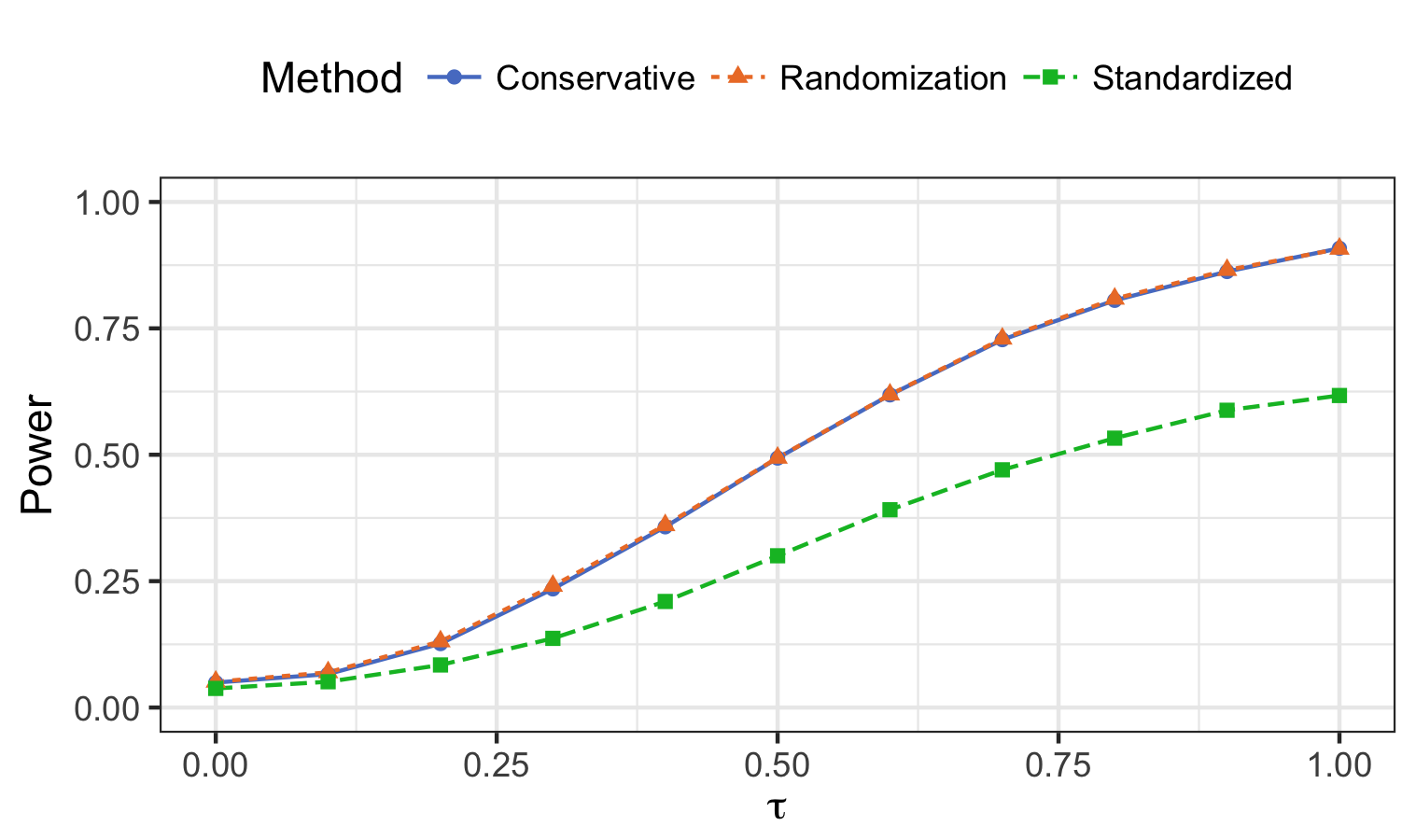
For $\widehat{\bar{\tau}}_{0}$ and $\widehat{\bar{v}}_{0}$ as $\bar{\tau}_{0}$ varies

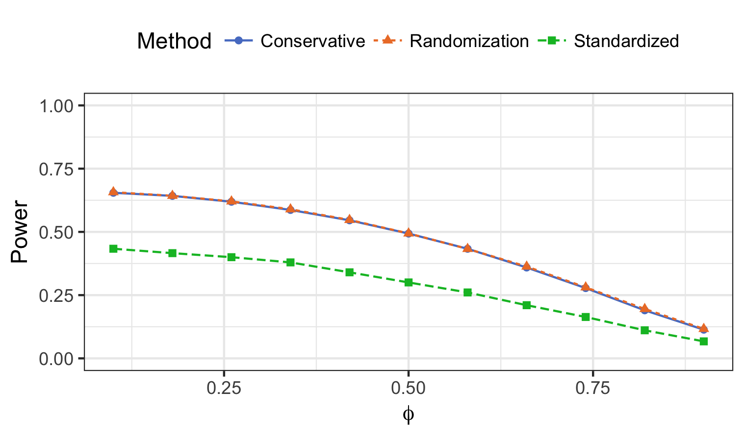
For $\widehat{\bar{\tau}}_{1}$ and $\widehat{\bar{v}}_{1}$ as $\phi$ varies

Figure 8: The two plots shows the relative power for the three tests as the treatment effect increases for fixed $\phi=0.5$ (left) and as the $\phi$ parameter increases for fixed $\tau=0.5$ (right). The conservative test performs only slightly worse that the exact randomization test. The noise distribution is Gaussian with variance 1.

It shows that the standardized test has worse power than the exact and the conservative tests discussed above.

B.4.2 Empirical results 

We have repeated our empirical analysis using the standardized statistics.

Market	Average Slippage		$\hat{\bar{\tau}}_{0}$	p.val	$\hat{\bar{v}}_{0}$	p.val
	A	B
1	1.48	2.29	0.52	0.628	0.03	0.678
2	4.11	3.35	-1.80	0.315	0.03	0.741
3	-0.05	1.07	0.54	0.634	0.01	0.893
4	3.38	3.23	0.36	0.900	-0.03	0.912
5	0.57	0.63	-0.42	0.743	-0.03	0.671
6	-1.48	3.72	5.26	0.008	0.25	0.034
7	1.99	1.64	-0.19	0.881	0.06	0.374
8	-0.08	-0.07	0.01	0.996	0.06	0.557
9	-2.19	0.64	2.60	0.000	0.14	0.005
10	0.80	2.10	0.57	0.603	0.06	0.143
Overall	0.55	1.60	1.11	0.010	0.060	0.003

Table 4: Randomization based inference results, “B” is considered treatment and “A” is considered control. The overall $p$-values (p.val) were obtained using the randomization method.

The basic results are given in Table 4.  The pooled results are given in Table 5.  Overall, the standardized statistics are broadly in line with the unstandardized ones.

	Unstandardized		Standardized
$p$	$\widehat{\bar{\tau}}_{p}$	p.val	$\widehat{\bar{v}}_{p}$	p.val
0	1.108	0.010	0.060	0.003
1	-0.337	0.396	0.001	0.953
2	-0.494	0.161	-0.044	0.018
3	-0.029	0.933	-0.025	0.167
4	-0.046	0.882	-0.020	0.278

Table 5: The results from the pooled hypothesis test for the 10 Markets for $\widehat{\overline{\tau}}_{p}$ and $\widehat{\overline{v}}_{p}$.

B.5 Definition of financial slippage

We write the time the $t$-th randomization is carried out as $\zeta_{0,t}$ and at precisely that time the mid-price of the asset (the average of the best advertised bid (buying price) and offer (selling price)) is recorded as $P_{\zeta_{0,t}}^{mid}$.  The trading performance will be compared to this mid-price.  Let $b_{t}=1$ if this is a sell order and $b_{t}=-1$ if this is a buy order.

Suppose the trades are made at times $\zeta_{j,t}$ where $j=1,2,...,J_{t}$ and the fraction of the fill of $t$-th order achieved on the $\zeta_{j,t}$-th trade is $v_{j,t}>0$.  All trades are filled so $\sum_{j=1}^{J_{t}}v_{j,t}=1$. Then the “slippage” rate, in terms of basis points (one basis point is 0.01%), will be $Y_{t}^{\text{obs}}=b_{t}r_{t}$ where writing $P_{\zeta_{j,t}}$ as the price of the trade made by the company (not the mid-price) at time $\zeta_{j,t}$,

$$r_{t} = 10000\frac{1}{P_{\zeta_{0,t}}^{mid}}\left(\sum_{j=1}^{J_{t}}v_{j,t}P_{\zeta_{j,t}}-P_{\zeta_{0,t}}^{mid}\right)=10000\sum_{j=1}^{J_{t}}v_{j,t}\frac{P_{\zeta_{j,t}}-P_{\zeta_{0,t}}^{mid}}{P_{\zeta_{0,t}}^{mid}}$$

$$= \sum_{j=1}^{J_{t}}v_{\zeta_{j,t}}r_{\zeta_{j,t}},\quad r_{\zeta_{j,t}}=10000\frac{P_{\zeta{{}_{j,t}}}-P_{\zeta_{0,t}}^{mid}}{P_{\zeta_{0,t}}^{mid}}.$$

Thus $r_{t}$ is a volume weighted average price (VWAP) minus the mid-price scaled by mid-price (e.g. Berkowitz et al. (1988) and Calvori et al. (2013)).

B.6 Simulation study extra figures

$\widehat{\bar{\tau}}_{0}$ $\mu_{1}=0.0$, $\mu_{0}=0.0$

$\widehat{\bar{\tau}}_{0}^{(1)}$

B.7 Extra figures from the empirical example

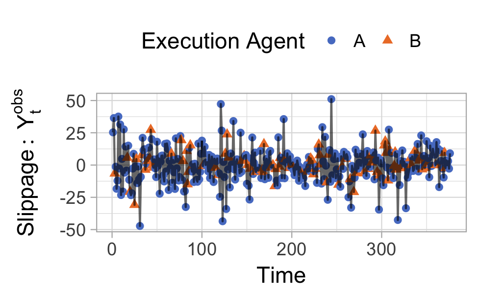
Market 3

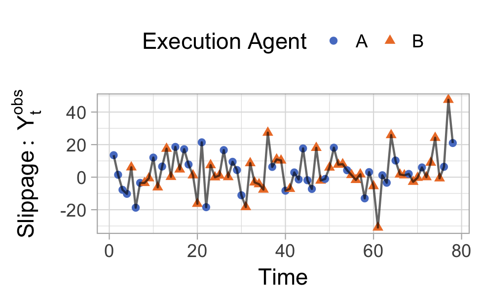
Market 4

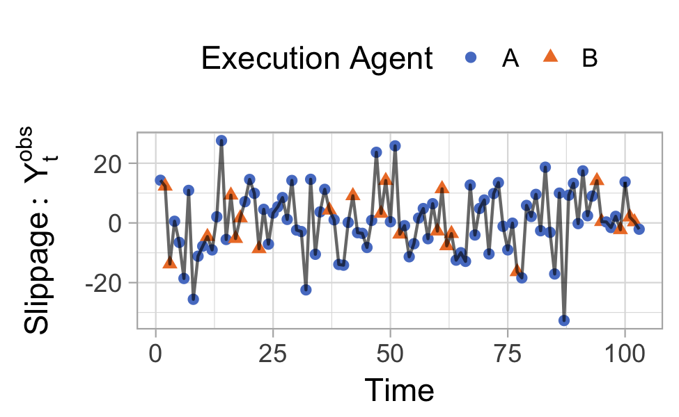
Market 5

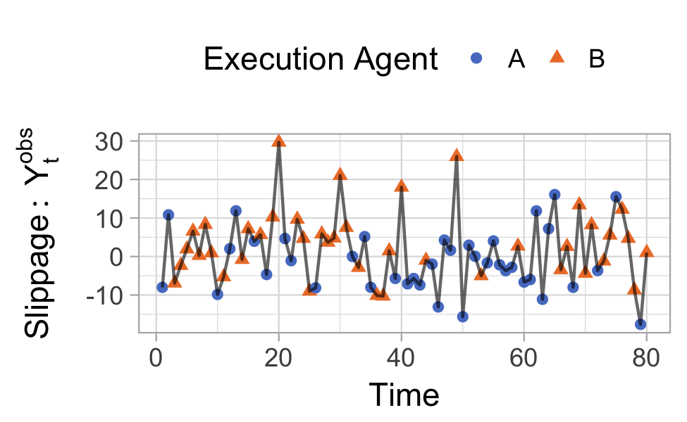
Market 6

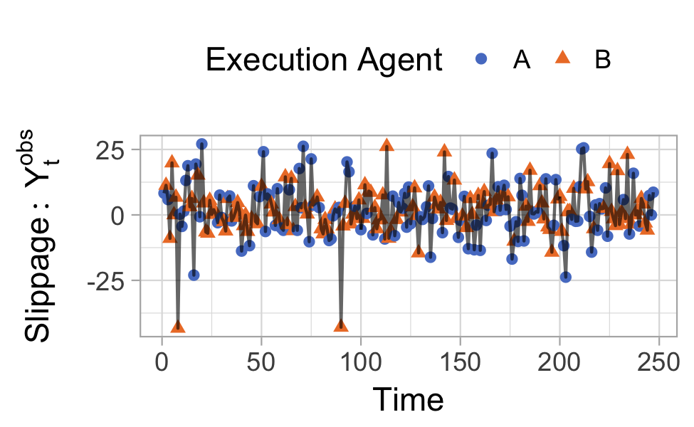
Market 7

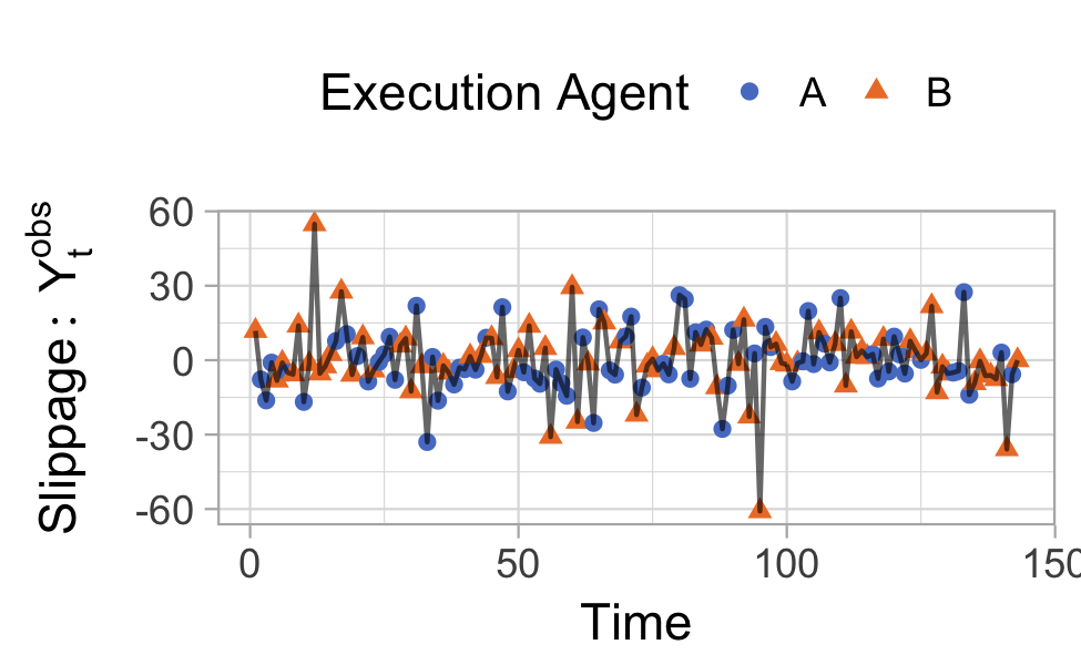
Market 8

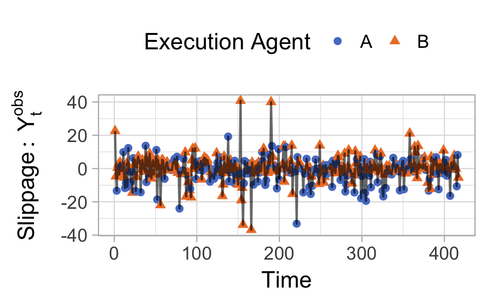
Market 9

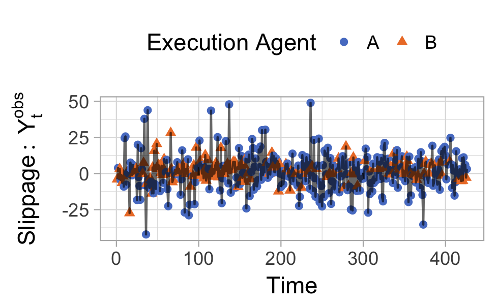
Market 10

Figure 11: Slippage $Y_{t}^{\text{obs}}$ as a function of time for eight markets, red indicates agent A and blue indicated agent B.

References

- Abbring and van den Berg (2003) Abbring, J. H. and G. van den Berg (2003). The nonparametric identification of treatment effects in duration models. Econometrica 71, 1491–1517.
- Angrist et al. (2017) Angrist, J. D., Ò. Jordà, and G. M. Kuersteiner (2017). Semiparametric estimates of monetary policy effects: string theory revisited. Journal of Business & Economic Statistics.