Halo intrinsic alignment: dependence on mass, formation time and environment

Abstract

In this paper we use high-resolution cosmological simulations to study halo intrinsic alignment and its dependence on mass, formation time and large-scale environment. In agreement with previous studies using N-body simulations, it is found that massive halos have stronger alignment. For the first time, we find that for given halo mass, older halos have stronger alignment and halos in cluster regions also have stronger alignment than those in filament. To model these dependencies we extend the linear alignment model with inclusion of halo bias and find that the halo alignment with its mass and formation time dependence can be explained by halo bias. However, the model can not account for the environment dependence, as it is found that halo bias is lower in clusters and higher in filaments. Our results suggest that halo bias and environment are independent factors in determining halo alignment. We also study the halo alignment correlation function and find that halos are strongly clustered along their major axes and less clustered along the minor axes. The correlated halo alignment can extend to scale as large as $100h^{-1}$Mpc where its feature is mainly driven by the baryon acoustic oscillation effect.

1. Introduction

Observational data from large sky surveys have clearly shown that galaxies are aligned with each other and also with the matter distribution on large-scale structure. On galactic scales, the satellite galaxies are aligned with the major axis of the central galaxy (e.g., Sales & Lambas (2004), Brainerd (2005), Yang et al. (2005)). On scales larger than a few $\,h^{-1}\text{Mpc}$, the spin of spiral galaxies are also correlated (e.g., Pen et al. (2000); Lee (2011)), so is for the shape of galaxies (Brown et al. (2002), Hirata et al. (2004), Heymans et al. (2004), Okumura et al. (2009), Faltenbacher et al. (2009), Joachimi et al. (2011), Joachimi et al. (2013), Singh et al. (2015)). The galaxy shape alignment can be extended to very large scale around 70-100$\,h^{-1}\text{Mpc}$ (Smargon et al. (2012), Li et al. (2013)). Galaxies are also found to align with the cosmic web (e.g., Lee & Erdogdu (2007), Zhang et al. (2013)), though with dependence on galaxy mass and morphology (Tempel & Libeskind (2013)). For a recent review on the various kinds of galaxy alignment, we refer the readers to the papers by Joachimi et al. (2015) and KANG et al. (2017) (but in chinese language).

Among the above various galaxy alignments, the shape correlation between galaxies on large scales is of great importance as it is a major contamination to weak lensing surveys and precision cosmology requires a good understanding of galaxy alignment (e.g., Kirk et al. (2012)). N-body simulations have been extensively used to study the intrinsic alignment (IA) of dark matter halos since the beginning of this century (e.g., Croft & Metzler (2000); Heavens et al. (2000); Jing (2002)). These studies found that halo IA is strong in massive halos and a useful fitting formula is given in Jing (2002). To explain the observed galaxy IA at low-redshifts, a mis-alignment between galaxy shape and halo has to be included (e.g., Kang et al. (2007); Faltenbacher et al. (2009); Okumura et al. (2009); Li et al. (2013); Joachimi et al. (2013)). However, it is not clear how the mis-alignment between halo and galaxy shape should depend on galaxy properties. In recent years, cosmological hydro-dynamical simulations are also used to directly measure galaxy IA and its dependence on galaxy mass, luminosity and redshift (e.g., Dubois et al. (2014); Tenneti et al. (2015); Velliscig et al. (2015); Chisari et al. (2016); Hilbert et al. (2017)). These studies have found in common that galaxy IA depends on luminosity and morphology. However, due to the difference of the adopted cosmology and the uncertainty of implemented star formation physics, the predicted galaxy IA are still different in detail from the hydro-dynamical simulations. For a review on the progress of measuring galaxy/halo IA using simulations, please refer to the paper by Kiessling et al. (2015).

For a better understanding of the physical origin of halo/galaxy IA, we need a theoretical model which can recover the halo/galaxy IA as seen in simulations. The linear alignment model (Hirata & Seljak (2004)) is developed based on the tidal theory (e.g., Catelan et al. (2001)) with major assumption that halo/galaxy shape is determined by the local tidal field. Subsequently, the linear model is improved on non-linear scales (Blazek et al. (2011)) and a more comprehensive halo model is also developed (Schneider & Bridle (2010)). However, in these analytical models the halo bias is neglected, and galaxy bias is presented only in the second order of power spectrum for galaxy IA. Thus, it is still not clear if the analytical model can account for the simulated galaxy IA in detail, such as the dependence on galaxy formation time and environment. As a further step to model the galaxy IA in detail, in this paper we use N-body simulation to study halo IA, especially we present the first measurement of halo IA with dependence on halo formation time and cosmic environment. We also investigate if the linear model with inclusion of halo bias can explain the halo IA with dependence on formation time and cosmic environment.

Our paper is organized as follows. In Sec.2 we introduce our simulation data, the method to clarify the large scale structure and the modified analytical model to describe the halo IA. In Sec.3 we present the simulation results on halo IA with dependence on halo mass, formation time and large-scale environment, and we also show how our slightly modified linear tidal model can fit the mass and formation time dependence of halo IA. In Sec.4 we present the results on the halo alignment correlation functions and investigate the origin behind the oscillation of halo IA on very large scales. In Sec.5 we summarize our results and briefly discuss their implications.

2. Methodology

In this section, we introduce the simulation data, calculation of halo IA and definition of the large-scale environment of the halo. We will also show the slightly modified linear tidal model to describe the halo IA in 3D coordinate measured from our simulations.

We use two cosmological N-body simulations in this paper. One is the Pangu simulation, carried out by the Computational Cosmology Consortium of China (Li et al. (2012), hereafter this simulation is abbreviated as C4), which simulated the evolution of the universe in a cubic box with each side of 1000$\,h^{-1}\text{Mpc}$. The other simulation is a part of the ELUCID project (Wang et al. (2014, 2016), Li et al. (2016)) with box-size 500$\,h^{-1}\text{Mpc}$ (Hereafter L500). Both simulations are run by the GADGET-2 code (Springel (2005)) with $3072^{3}$ particles and the cosmological parameters can be found in Table 1. Note that the cosmological parameters in the two simulations are very close and we do not expect significant difference on our results, and we will also show comparison between them.

Table 1Simulation Parameters

Name	$\Omega_{M}$	$\Omega_{\Lambda}$	$\Omega_{b}$	h	L ($h^{-1}$Mpc)	$m_{p}(\,h^{-1}\text{M}_{\odot})$
L500	0.28	0.72	0.045	0.7	500	$3.4\times 10^{8}$
C4	0.26	0.74	0.045	0.7	1000	$2.5\times 10^{9}$

Using the friends-of-friends (FOF) algorithm with a linking length $b=0.2$ of the mean particle separation, we identified dark matter halos in both simulations. For each halo, we project its dark matter particles along one axis of the simulation box and calculate the halo’s reduced 2D moment of inertia tensor $I_{ij}$ (Bailin & Steinmetz (2005)) as,

$$I_{ij}=\sum_{k}\frac{m_{\alpha}x_{k,i}x_{k,j}}{x^{2}_{k}},\ \text{ with}i,j\in\{1,2\},$$ (1)

where $x_{k}$ is the distance of the $k$th particle to the halo center which is set as the position of the most bound particle. The eigenvalues $\lambda_{1},\lambda_{2}~{}(\lambda_{1}>\lambda_{2})$ of the inertia tensor then define the axis ratio $q=\lambda_{2}/\lambda_{1}$. Then, following Heavens et al. (2000) and Jing (2002), we define the halo shape by the ellipticity vector,

$${\boldsymbol{\epsilon}}=\frac{1-q^{2}}{1+q^{2}}(\cos 2\alpha,\sin 2\alpha)^{T}=(\epsilon_{1},\epsilon_{2})^{T},$$ (2)

which in the complex form reads,

$$\epsilon=\epsilon_{1}+{\rm i}\epsilon_{2}=\frac{1-q^{2}}{1+q^{2}}\exp\left({\rm i}2\alpha\right).$$ (3)

where $\alpha$ is the position angle of the halo measured anti-clockwise from x-axis.

As pointed by earlier studies (Jing (2002); Bailin & Steinmetz (2005)), a lower limit of particle number ($\approx$ 300 particles) in the halo has to be used to get a converged shape measurement. To ensure a safer measurement, in this work we select halos with more than 500 particles. In addition, it is found that the halo shape is also dependent on the linking length to find halo in the FOF algorithm. Croft & Metzler (2000) had shown that this can lead to the discrepancy of halo IA at the low-mass end. We will later show comparison of our results with Jing (2002).

To define the local large-scale environment of a halo, we use the Hessian matrix of the density field at the position of the halo (e.g., Aragón-Calvo et al. (2007)). Adopting the Cloud-in-Cell (CIC) algorithm, the density field is smoothed via a length of $2\,h^{-1}\text{Mpc}$ and the Hessian matrix of the smoothed density field $\rho_{s}$ at halo position is described as,

$$H_{ij}=\frac{\partial\rho_{s}}{\partial x_{i}\partial x_{j}},$$ (4)

The eigenvalues of the Hessian matrix define the large-scale environment of the halo, and it can be classified into cluster, filament, sheet and void, depending on the sign of the eigenvalues. By ordering the eigenvalue as $\lambda_{1}>\lambda_{2}>\lambda_{3}$, the environment is linked as,

$$(-,-,-) \rightarrow$$ cluster

$$(+,-,-) \rightarrow$$ filament

$$(+,+,-) \rightarrow$$ sheet

$$(+,+,+) \rightarrow$$ void

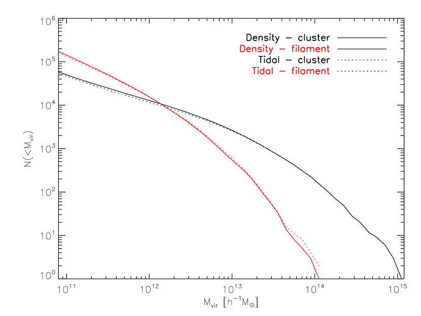
Figure 1.— The mass function of halos in clusters (black) and filaments (red) from L500 using Density-Hessian classification (solid) and Tidal-Tensor classification (dotted).

We note that this way of defining LSS environment is different from the tidal environment defined in Hahn et al. (2007) in which the Hessian of the potential (i.e., tidal field) is used and classification is done using an opposite signature of eigenvalues. In Fig. 1, we plot the halo mass function in cluster and filament environment from the two different classification schemes, and in Table 2, we list the ratio of each LSS environment under the two classification methods. It is seen from Fig. 1 that the halo mass functions agree well in the two environments. By checking the environment of each halo, we find that 77% of all halos keep their environment unchanged and 23% of them changed when changing the classification method. For this paper, we will adopt the density-Hessian classification scheme. We will still be using the density Hessian as “tidal field” in our context, but the reader should be aware of the mentioned difference when comparing with previous studies which adopts tidal tensor. We also direct the reader to Libeskind et al. (2017) for detailed comparison and discussions on different LSS classification schemes.

Table 2LSS Environment Ratios (%)

	Cluster	Filament	Sheet	Void
Density Hessian	20.0359	61.8152	17.7563	0.3926
Tidal Field	19.3583	58.0268	21.1922	1.4227
In Total	Same	Different
	76.9173	23.082

Basically the environment of the halo is related to its mass: usually massive halos live in cluster regions and low-mass halos live in sheets and voids. The halo shape is also closely related to the eigenvector of the environment, for a short summary of how halo shape is related to the environment and its physical origins, we refer the reader to the paper by Kang & Wang (2015) and Wang & Kang (2017) and references therein.

Now we describe how the halo IA is usually defined in the weak lensing theory. Following the conventional description (Heavens et al. (2000); Jing (2002)), for a pair of halos (halo 1 and halo 2), let $w_{1}=x_{1}+{\rm i}y_{1}$ and $w_{2}=x_{2}+{\rm i}y_{2}$ be projected positions of two halos in the complex plane, and call the direction defined by $\varphi=\arg(w_{2}-w_{1})$ (anti-clockwise from the positive real axis) as the separation direction . Then, for this pair of halos we can define the tangential shear $\gamma_{t}$ and the cross shear $\gamma_{x}$

$$\gamma_{t}=-\operatorname{Re}\left(\epsilon\exp(-2{\rm i}\varphi)\right),~{}~{}\gamma_{\times}=-\operatorname{Im}\left(\epsilon\exp(-2{\rm i}\varphi)\right),$$ (5)

where $\epsilon$ is the complex shear of a given halo defined in Eq. 3. The halo IA is usually defined as $c_{11}(r)=\langle\gamma_{t}(0)\gamma_{t}(r)\rangle$, sometimes also labeled as $\eta_{1}(r)$, and $\langle\gamma_{\times}(0)\gamma_{\times}(r)\rangle$ is labeled as $c_{22}(r)$.

By assuming that galaxy shapes are determined by their local tidal shear, the linear alignment model (Hirata & Seljak (2004)) suggests that galaxy ellipticity is:

$$\gamma^{I}_{(t,\times)}=-\frac{C_{1}}{4\pi G}(\nabla_{x}^{2}-\nabla_{y}^{2},2\nabla_{x}\nabla_{y})S[\Psi_{P}],$$ (6)

Where $C_{1}$ is a free parameter which can be determined by fitting the observed galaxy IA. Up to now, most studies have determined the value of $C_{1}$ by fitting the IA correlation of low-z massive galaxies (luminous red galaxies) as a whole. So it is not clear how the normalization will vary as a function as galaxy luminosity. Also as the fitting is for galaxy IA, it is not clear if the tidal model (Eq. 6) can describe the IA of dark matter halo and its mass dependence.

To investigate the impact of galaxy IA on probing cosmology, it is important to measure the IA signal in the shear correlation function, which is defined as,

$$\xi_{\pm}(\theta)=\langle\gamma_{t}\gamma_{t}\rangle(\theta)\pm\langle\gamma_{\times}\gamma_{\times}\rangle(\theta)$$ (7)

where $\theta$ is the angular separation on the sky. Blazek et al. (2011) (Eq. 3.5 therein) showed that under the linear alignment model, the projected tangential and cross components of the shear correlation function to the linear order is,

$$\langle\gamma\gamma\rangle^{LA}_{(tt,\times\times)}(r_{p}) =\frac{1}{{2\pi^{2}}}\left(\frac{C_{1}\rho_{m,0}}{D(z)}\right)^{2}\int d\kappa dk_{z}\frac{\kappa^{5}}{k^{4}k_{z}}P_{\delta}(k,z)$$

$$\times\sin(k_{z}\Pi_{\rm max})\left[J_{0}(\kappa r_{p})\pm J_{4}(\kappa r_{p})\right].$$ (8)

However, for $c_{11}$ in Jing (2002), the correlation of projected shapes are calculated at each 3D distance between halo pairs. We explicitly calculate our model prediction for $c_{11}$ by first performing the integral $\xi_{\pm}(r)=\int_{0}^{\pi}\xi_{\pm}(r_{p}=r\sin\phi,\Pi=r\cos\phi)~{}{\rm d}\phi$. Then, after analytically integrate over azimuthal angles, we obtain the final formula

$$\xi_{-}(r)=\left(\frac{C_{1}\rho_{m,0}}{D(z)}\right)^{2}\frac{1}{4\pi}\int_{0}^{\infty}{\rm d}k~{}\frac{\mathcal{P}_{\delta}(k)}{k}~{}\sqrt{\frac{2\pi}{kr}}~{}\frac{3\pi}{8}~{}J_{\frac{9}{2}}(kr),$$ (9)

and,

$$\xi_{+}(r) =\left(\frac{C_{1}\rho_{m,0}}{D(z)}\right)^{2}\frac{1}{4\pi}\int_{0}^{\infty}{\rm d}k~{}\frac{\mathcal{P}_{\delta}(k)}{k}~{}\sqrt{\frac{2\pi^{3}}{kr}}$$

$$\times\left(\frac{9}{280}J_{\frac{9}{2}}(kr)+\frac{4}{21}J_{\frac{5}{2}}(kr)+\frac{56}{105}J_{\frac{1}{2}}(kr)\right),$$ (10)

where $J_{n+\frac{1}{2}}$ is the Bessel function of half-integer order. Hence, by relation $c_{11}(r)=\langle\epsilon^{h}_{+}\epsilon^{h}_{+}\rangle(r)=\frac{1}{2}(\xi_{+}(r)+\xi_{-}(r))$, we now have the prediction of $c_{11}(r)$ from the linear alignment theory.

Since we are calculating the shear correlation functions at halo positions, we will be using $\mathcal{P}_{\delta,h}$ instead of $\mathcal{P}_{\delta}$ in the above equations. For halos at fixed mass, the power spectrum at halo position is $\mathcal{P}_{\delta,h}(M)=b_{h}^{2}(M)~{}\mathcal{P}_{\delta}$, where $b_{h}$ is the halo bias. The fact that we will be calculating ellipticity correlation of halos within different mass ranges suggests that we should extend to, $\mathcal{P}_{\delta,h}(M_{h}\geq M)$, which by conditioning on halos with mass $M_{h}\geq M$ and to linear order:

$$\mathcal{P}_{\delta,h}(M_{h}\geq M)=b_{h}^{2}(M_{h}\geq M)\mathcal{P}_{\delta},$$ (11)

Therefore, we get the mass-dependent $c_{11}$ for halos

$$c_{11}(r,\geq M)=\left(\frac{\int_{M}^{\infty}b_{h}(M^{\prime})\Phi(M^{\prime}){\rm d}M^{\prime}}{\int_{M}^{\infty}\Phi(M^{\prime}){\rm d}M^{\prime}}\right)^{2}\langle\epsilon^{h}_{+}\epsilon^{h}_{+}\rangle(r),$$ (12)

where $\Phi(M)$ is the halo mass function which can be obtained for given cosmology.

3. Dependencies of Halo Intrinsic Alignments

3.1. Mass dependence of halo IA

In Sec.2 we have outlined the theoretical model for halo IA and in this section, we compare the simulation results to model predictions to see if the linear model can fit the mass dependence of halo IA.

First we note that, as pointed by Jing (2002), when calculating $c_{11}$ from Eq. 5, not only the direction of the halo shape is correlated, the ellipticity of the halo is also taken into account (the term $(1-q^{2})/(1+q^{2})$), so is for the theoretical description by Eq. 6. So basically that is the ellipticity weighted $c_{11}$. In fact we can also only consider the orientation correlation by assuming that $q=0$ (unweighted by ellipticity) in the simulations. In Fig.2 we show the measured weighted and unweighted $c_{11}$ for halos larger than given mass in the left and right panel. The circles are from L500 simulation and diamonds are from C4. For clarity, the result for different halo mass bin has been shifted by different factors. It is found that the results from the two simulations agree quite well for both weighted and unweighted correlations. For the following we will only show results from the L500 simulation unless otherwise stated.

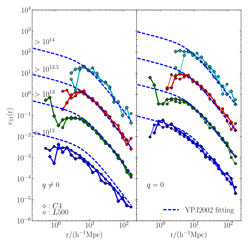
Figure 2.— The ellipticity correlation function $c_{11}$ of halos from L500 (circles connected with solid lines) and C4 (diamonds connected with solid lines) simulations at $z=0$. The results for different halo mass bins ($\log(M/(h^{-1}M_{\odot}))>12,13,13.5,14$ (from bottom to top) have been multiplied by 1, 10, 100 and 1000 respectively for clarity. The fitting formula from Jing (2002) is shown as blue dashed lines in both panels. Left: the ellipticity weighted correlation. Right: no ellipticity included, only halo orientation is correlated.

Jing (2002) measured the weighted $c_{11}$ from their simulation, and found it can be well fitted by a simple formula with mass dependence as,

$$c^{\text{YPJ}}_{11}(\geq M_{\text{h}};r)=\frac{3.6\times 10^{-2}\left(\frac{M_{\text{h}}}{10^{10}\,h^{-1}\text{M}_{\odot}}\right)^{0.5}}{r^{0.4}\left(7.5^{1.7}+r^{1.7}\right)},$$ (13)

We plot their fitting as dashed lines in Fig. 2. It is worth noting that their fitting formula was intended for FoF halos with a linking length with $b=0.1$. As pointed in Jing (2002) the mass of FOF halo using $b=0.1$ is about half of the FOF halo mass with $b=0.2$. Therefore, the dashed lines here are plotted using the fitting formula but with half of the halo mass in our simulation (with $b=0.2$). It is found that the fitting formula can also well fit our results except at the low mass end where our $c_{11}$ is lower than that of $c_{11}^{\text{YPJ}}$. It indicates that $c_{11}$ in our simulation has a slightly stronger mass dependence. As shown by Croft & Metzler (2000), such a slight difference is expected as the measured halo shape is slightly different with different link length, especially for low-mass halos. In addition, given the additional difference in cosmological parameter, simulation box and resolution, we believe such a slight difference is acceptable. The right panel shows that without considering the halo ellipticity, our $c_{11}$ agrees with the fitting formula much better. We also note that for the unweighted $c_{11}$ the fitting formula is multiplied by a factor of $\sim 6$ to produce good match with the data, similar to the finding of Okumura et al. (2009). The fact that the fitting formula at $q=0$ works well also confirms that the difference seen in the left panel for low mass halos mainly comes from randomness of halo ellipticities at low mass.

Figure 3.— The ellipticity correlation function $c_{11}$ of halos at two redshifts. Left: correlation at $z=0$. Similar to Fig. 2, but the dashed lines are the theoretical model predictions. Right panel: the correlation at $z=1$.

In Fig. 3 we compare our simulation results to the theoretical model. The left panel is the same as that of Fig. 2, but now the dashed lines are the model predictions (Eq. 12). For the theoretical model we adopted the halo bias from Pujol & Gaztañaga (2014) and the halo mass function $\Phi(M)$ is taken from our simulation. For the power spectrum we used the nonlinear power spectrum from halofit Peacock & Smith (2000) adhering to the L500 cosmological parameters. In addition, to better match the real power spectrum in simulation we added Cloud-In-Cell window function Cui et al. (2008) with a 2$\,h^{-1}\text{Mpc}$ smoothing kernel in the computation. We tune the free model parameters for weighted and unweighted $c_{11}$ respectively to better match the simulation results for the highest mass bin (upper line). It is seen that the simulation results can be well matched by the theoretical predictions, indicating that it is mainly the halo bias accounting for the mass dependence of halo IA, $c_{11}$. Again we find that the mass dependence in the simulation is slightly stronger than the linear tidal model. The right panel shows a better agreement on the unweighted $c_{11}$ with the model. The better agreement on the unweighted $c_{11}$ indicates that the correlation between direction of the halo (major axis) is better described than the ellipticity by the linear tidal model.

In the right panel of Fig. 3 we plot the $c_{11}$ at $z=1$ as an additional test of the linear tidal model. Amazingly, the agreement at higher redshift is also good and even better than the $z=0$ results. This is also expected as it is known that the tidal field at earlier time can be better described by the linear theory. Following equation (B.5) in Joachimi et al. (2011), we also note that the ratio between the free parameter in our unweighted model $\frac{C_{1}(z=1)\rho_{m,0}}{D(z=1)}/\frac{C_{1}(z=0)\rho_{m,0}}{D(z=0)}\approx 1.40$ is slightly lower than the ratio from the linear growth factor ${D(z=0)}/{D(z=1)}\approx 1.61$. This indicates that the redshift evolution can be roughly captured by the power spectrum at different redshift, yet there is still other factors which is absorbed in the normalization factor $C_{1}$ which should slightly depend on redshift.

3.2. Formation time and environment dependence

It is well known that halo properties, such as concentration and bias, are closely related to halo formation time (e.g., Navarro et al. (1997); Gao et al. (2004)). In this section we investigate whether the halo IA is also dependent on halo formation time. Here, we use the most common definition of formation time, $z_{f}$, at which the mass assembled in the main progenitor of a halo is half of its present (z=0) mass, i.e., $M_{h}(z=z_{f})=\frac{1}{2}M_{h}(z=0)$. As there is a strong correlation between halo formation time and its mass (e.g., Navarro et al. (1997)), we select halos in a few narrow mass bins and divide the 20% oldest and youngest halos into the old and young samples. In addition, as we will soon see that halo IA is also dependent on their environment, we refine the old and young halo samples to make sure they have the same distributions of cosmic environment as identified in Sec. 2.

In Fig. 4, we plot the unweighted $c_{11}$ signal for old and young halos in a few mass bins. It is seen that in low-mass bins ($\lg M<12.5$), old halos have stronger alignment than young halos and at intermediate scales $\sim 10Mpc/h$, the IA of old halos is around 2 times of the young halos. For massive halos (lower right panel) the difference between the two samples is small. This trend can be quantitatively explained by our tidal alignment model (Eq. 12) with inclusion of halo bias. These difference of halo IA in old and young halos are in good agreement with the dependence of halo bias on formation time as found by Gao et al. (2004).

Previously, to explain the mass dependence of halo IA, Smith & Watts (2005) argued that massive halos are stronger aligned as they are formed later, so they have less time to virialize and still keep the memory of the tidal field that they collapsed within. Our results above show that halo IA is dependent on both halo mass and the formation time, and it can be understood using our linear model in terms of halo bias with its dependence on mass and formation time separately.

Figure 4.— Unweighted halo ellipticity correlation function $c_{11}$ ($q=0$) at $z=0$ for old and young halos in a few mass bins. The difference between their correlation is decreasing with halo mass, consistent with the age dependence of halo bias as function as halo mass.

Many studies have shown that halo spins are correlated with the large-scale environment (e.g., Hahn et al. (2007), Kang & Wang (2015) and references therein). There is also a strong possibility that halos IA will also depend on the large-scale environment. In this part we compare the halo IA in different environments, mainly in cluster and filament. We select question halos with mass $>10^{12}\,h^{-1}\text{M}_{\odot}$, and label those in cluster and filament environment as pure $Q_{\text{clu}}$ and pure $Q_{\text{fil}}$ sample respectively. As halo mass is strongly correlated with its environment (e.g.,Hahn et al. (2007)) that halos in cluster environment are usually larger, therefore, direct comparison of $c_{11}$ between these two samples will suffer from significant mass-dependence effect as seen in previous section. So we construct two control samples, $Q_{\text{clu}}^{\text{control}}$ and $Q_{\text{fil}}^{\text{control}}$ respectively, ensuring they have the same halo mass distribution as the pure cluster/filament samples, but regardless of their environment.

After eliminating the halo mass dependence, to see if there is additional difference in the formation time between the question and control samples, we plot their formation time distributions in Fig. 5. By comparing the solid and dashed lines, it is seen that under the same mass distribution the formation time is identical between the question and control sample. Previous work (e.g., Hahn et al. (2007)) have found for low-mass halo ($<10^{12}\,h^{-1}\text{M}_{\odot}$), the formation time has dependence on the environment, in which cluster halos form earlier than those in filaments and voids, but for massive halos there is no environmental dependence. As we are looking at halos larger than $10^{12}\,h^{-1}\text{M}_{\odot}$, our results agree well with their results. The formation time of halos in cluster environment is slightly lower than the halo in filaments, this is because the average halo mass in cluster is larger, so the formation time is lower.

Figure 5.— Formation time distribution for question (solid) and control (dashed) samples of halos in cluster and filament environment.

In Fig.6, we plot $c_{11}$ for the pure cluster/filament samples in solid lines and the control samples in dashed lines. The errorbars are taken from 10 realizations of the control samples. We find that under the same mass distribution, $c_{11}$ from halos in cluster environment (red solid line) is much stronger than the control sample which has a mixture of different environments (red dashed line). On the other hand, the $c_{11}$ for halos in filament (blue solid) is much weaker than that in the control samples (blue dashed). The difference between solid lines includes both mass and environment dependence. The fact that $c_{11}$ for $Q_{\text{clu}}^{\text{control}}$ is higher than that of $Q_{\text{fil}}^{\text{control}}$ is mainly due to the mass dependence.

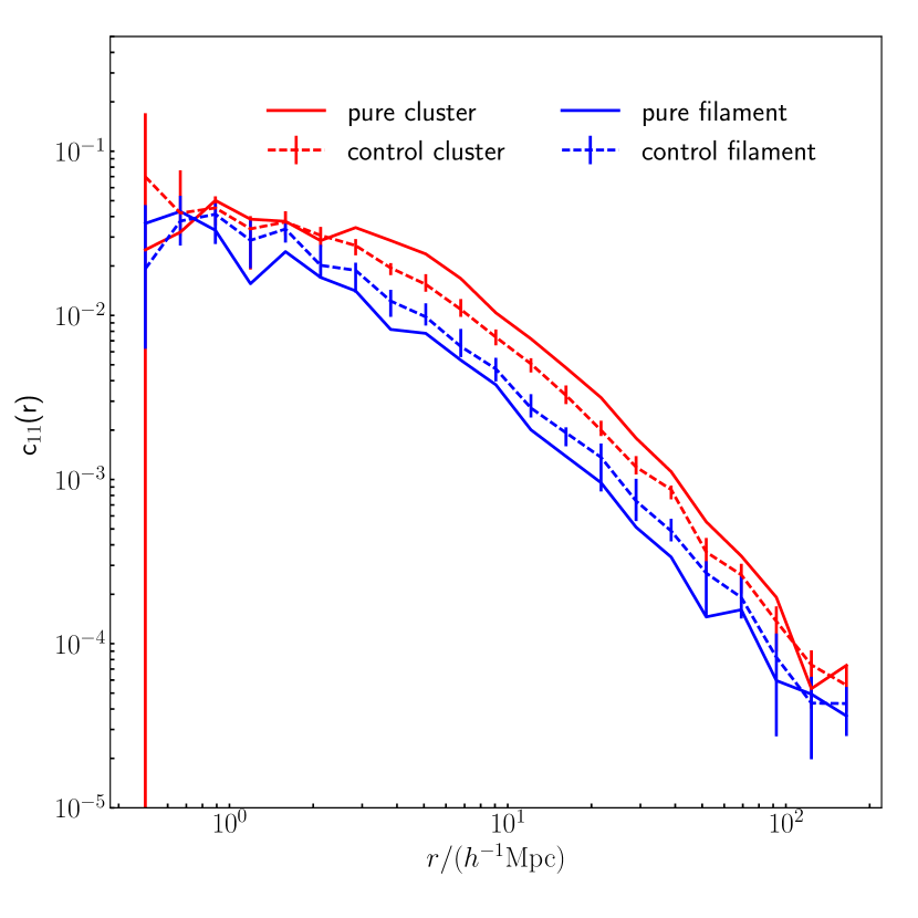
Figure 6.— Ellipticity correlations (unweighted) at $z=0$ for halos in cluster and filament environment. The results for question samples are shown in solid lines and control samples in dashed lines. The control samples have the same halo mass distribution as the corresponding question samples. The error bars are from 10 realizations of the control samples.

Figure 7.— The cross-correlations in different cosmic environment. The black dashed and dotted lines are the halo-mass cross-correlation for halos in cluster and filament, and red/blue lines are for the corresponding control samples. The black solid line is the auto-cross correlation of the background mass distribution. Clear cosmic environment dependence on large-scale is seen that cluster halos have lower clustering (bias) than the background mass distribution, and filament halos have higher bias.

In order to understand the origin of environment dependence of halo IA and to see if it can be explained by halo bias as introduced in our theoretical model in Sec. 2, here we investigate the halo bias in different environment. We calculate the cross-correlation function $\xi_{hm}$ between the halos and the dark matter particles. For references we also calculate the auto-correlation function $\xi_{mm}$ of the background particles.

In Fig. 7, we show the cross-correlations of halos in different environment with the background particles. Firstly we note that, below the scale $\sim 2\,h^{-1}\text{Mpc}$, the halo-matter cross-correlation function mainly describes the clustering of dark matter particles inside halos. Therefore, this part of the correlation function mainly depends on the average halo mass in the studied sample. Since the question and control samples have the same mass distribution, the clusterings on small scales are very similar between them.

On scales beyond $2\,h^{-1}\text{Mpc}$, the cross-correlation function then reflects the level of clustering between particles in different halos. It is found that halos in cluster environment (black dashed line) is less clustered than halos in filament environment (black dotted line). The control samples have similar clustering as the corresponding question samples on small scales, but on large scales they are similar to the background dark matter particles, and the control cluster sample (red dashed line) has slightly higher correlations than the control filament sample (blue dashed line) due to their higher average halo mass.

Figure 8.— The probability density function of the halo-tidal alignment in cluster (red) and filament (blue) environment in mass bins $M_{\text{halo}}>10^{12},10^{13},10^{13.5}h^{-1}M_{\odot}$ respectively.

The higher clustering on large scales for halos in filament than halos in cluster is unexpected. We note that it is not due to the formation time difference between the two sample, as Fig. 5 shows that their formation time distributions are very similar. Interestingly, in a recent paper by Borzyszkowski et al. (2016) from the ZOMG project, the author found that stalled (filament) halos has a larger halo bias $b_{h}>1$ than the accreting (cluster) halos with $b_{h}<1$. The environment dependence is also recently confirmed by Yang et al. (2017) who study the halo bias in much more detail using the ELUCID simulations, and they also find that cluster halos are less clustered on larger scale. More recently, Paranjape et al. (2017) has found some very interesting results. Although they used a different method to define the large-scale environment (the anisotropy factor $\alpha_{R}$), they found that halo bias evolves smoothly with $\alpha_{R}$, and in particular, halos in ‘isotropic’ (node) environment have a negative bias while those in ‘anisotropic’ (filament) environment have a positive bias (see their Fig.12). This is qualitatively in agreement with our results in Fig. 7. In general, our results agree with the recent findings.

The fact that halo bias is higher in filament and lower in cluster is opposite to the trend of environment dependence seen in Fig. 6, and therefore we cannot use the halo bias term in our theoretical model to explain the environment dependence in halo IA. These two opposite trends for large-scale environment dependence also suggests that additional factors other than halo bias must be taken into account to understand this difference. In particular, these factors need to produce a significant difference in halo IA between cluster and filament to overcome any halo bias effect and result in the final $c_{11}$ that we see in Fig. 6.

One of such potential factors is the level of alignment between halo orientation and the large-scale environment. The basic assumption in the linear alignment model (Hirata & Seljak 2004) is that halo shape is perfectly aligned with the tidal field. As reported in Zhang et al. (2015), and Kang & Wang (2015), although the halo shape is strongly correlated with the local tidal field, there is still a mis-alignment with dependence on halo mass and environment. Here we calculate the alignment between the major axis ($v_{1}$) of the halo shape and the direction of the tidal field, i.e., $e_{3}$ from the Hessian matrix, which is the direction of the slowest collapse direction (for detail, see Kang & Wang 2015). We calculate their alignment as,

$${\bf e}_{3}\cdot{\bf v}_{1}=\cos\theta$$ (14)

where larger $|\cos\theta|$ means that the halo major axis is better aligned with the tidal field.

In Fig. 8, we plot the probability distribution of $|\cos\theta|$ for halos in three mass bins $M_{\text{halo}}>10^{12},10^{13},10^{13.5}h^{-1}M_{\odot}$ and in both filament and cluster environment. It is found that halos in clusters have a stronger alignment with local tidal field in all mass ranges. This result, given that large scale tidal field correlation underlies the large scale IA (Catelan & Porciani (2001)) , provides a plausible reason of why the halo IA being stronger in clusters and weaker in filaments. We believe this effect should be taken into account to fully explain the environment dependence of halo’s intrinsic alignment. In this paper we do not study this effect in details.

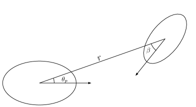
Figure 9.— Left: Illustration of the pointing angle $\theta_{p}$ and $\beta$; Right: Exaggerated illustration of the alignment correlation function.

4. The Alignment Correlation Function

Figure 10.— The halo alignment correlation functions. Upper panel: halo ACFs along different alignment angles. Red lines are for halos in cluster environment and blue for filament environment. Dashed lines are for correlations along the major axes of the halos ($0^{\circ}<\theta_{p}<30^{\circ}$) and dotted lines are for correlations along the minor axes of the halos ($60^{\circ}<\theta_{p}<90^{\circ}$). Black lines are for halos with no limit on the alignment angle. Lower panel: the ratio between halo ACF along different angles to the halo correlations with no limit on the alignment angle.

In Sec.3, we have shown the dependence of halo IA and comparison between simulation results with theoretical model predictions. There the halo IA is defined in a way similar to the one often used in weak lensing analyses. In fact the halo alignment has been measured in another way, called alignment correlation function (ACF), in which the halo clustering is a function of the direction along one halo axis (e.g., Faltenbacher et al. (2009)). Although the ACF and halo IA can be connected (especially GI term Blazek et al. (2011)), the ACF provides more direct insight on how halos/galaxies are correlated along their major or minor axes. An illustration of the ACF statistic is shown in Fig. 9 where $\theta_{p}$ is the angle between the major axis of a halo and the separation vector to another halo.

Given a sample of halos in question (sample Q) which is a subset of the reference sample G, the ACF $\xi(\theta_{p},r)$ is defined as (Faltenbacher et al. (2009)),

$$\xi(\theta_{p},r)=\frac{N_{R}}{N_{G}}\frac{QG(\theta_{p},r)}{QR(\theta_{p},r)}-1,$$ (15)

where R is a random sample.

The halo and galaxy ACFs have been measured in a few studies (Faltenbacher et al. (2009), Smargon et al. (2012), Li et al. (2013), Chisari et al. (2016), Chisari et al. (2015)). Li et al. (2013) showed the direct measurement of the ACF using CMASS galaxy catalogue, and in the meantime calculated the ACF for dark matter halos using cosmological simulation. They found evidence that galaxies and halos are more clustered than the average within a spanned region $\theta_{p}=(0^{\circ},30^{\circ})$ around the major axis and less clustered within $\theta_{p}=(60^{\circ},90^{\circ})$ at almost all scales. Furthermore, they found the correlation can be seen up to very large scales at around $70\,h^{-1}\text{Mpc}$. The results of Li et al. (2013) motivate us to study halo ACFs with their dependence on environment and investigate the origin of the correlation on very large scales.

Here we present an investigation on the environment dependence of halo ACF. In order to look for signals on very large scales, we use the full halo sample in the C4 simulation with box-size of $1h^{-1}{\rm Gpc}$ at $z=0.6$ (to match the Li et al. (2013) data from observations) as the reference sample G ($N_{G}=12,640,839$), and we use the set of halos with mass $M_{h}\geq 10^{12}\,h^{-1}\text{M}_{\odot}$ as sample Q. The random sample R is generated with $N_{R}/N_{G}=10$. We divide halos in sample Q into two samples, $Q_{clu}$ and $Q_{fil}$, based on their environment identified as cluster and filament. In the upper panel of Fig.10 we plot the ACFs for these samples.

Fig. 10 shows a few interesting features. First, it is found that without limitation on the alignment angle $\theta_{p}$, the halo ACF in cluster (red solid line) is lower than halos in filament (blue solid line). This is consistent with the results in Fig. 7 although there it plots the cross correlation between halo and dark matter and here we show the halo-halo cross-correlation. The halo ACF also displays a peak at around $110\,h^{-1}\text{Mpc}$, which is exactly the signal from the baryon acoustic oscillations (BAO). Secondly, it is found that in agreement with Li et al. (2013) the halo ACF with $0^{\circ}<\theta_{p}<30^{\circ}$ (dashed lines) is higher in both filament and cluster environment than the average, indicating that halo clustering is enhanced along their major axes. Accordingly, the clustering is decreased with $60^{\circ}<\theta_{p}<90^{\circ}$. An illustration of this effect is seen in the right panel of Fig. 9.

In the lower panel of Fig. 10 we show the ratio between halo ACFs along different alignment angles with the average ACFs in the cluster and filament environment, respectively. The dashed lines are for halos clustering along the major axes ($0^{\circ}<\theta<30^{\circ}$) and the dotted lines are for results along the minor axes of the halos ($60^{\circ}<\theta_{p}<90^{\circ}$). It is seen that although the halo ACF is lower in cluster, but the correlation along the major axis is significantly enhanced in cluster than in filament. It is also interestingly found that the clustering along the minor axes will become negative at some scales with dependence on halo environment. For example, for halos in cluster the ACF is negative at $r>35\,h^{-1}\text{Mpc}$ and reaches the lowest dip at around $90\,h^{-1}\text{Mpc}$ after which it increases to the peak at around $110\,h^{-1}\text{Mpc}$. For halos in filament, the clustering along minor axes becomes negative at around $70\,h^{-1}\text{Mpc}$ and reach a dip at around $90\,h^{-1}\text{Mpc}$. These results indicate that halo in clustering environment has a strong dependence on the alignment angle.

In addition to the halo ACF, we also calculate the alignment signal $\cos(2\theta_{p})$ over correlated pairs, which is defined in Faltenbacher et al. (2009) as

$$\langle\cos(2\theta_{p})\rangle_{\text{cor}}(r)=\frac{\int_{0}^{\pi/2}\cos(2\theta_{p})\xi(\theta_{p},r){\rm d}\theta_{p}}{\int_{0}^{\pi/2}\xi(\theta_{p},r){\rm d}\theta_{p}},$$ (16)

and is estimated by

$$\langle\cos(2\theta_{p})\rangle_{\text{cor}}(r)=\frac{QG_{\theta_{p}}(r)}{QG(r)-(N_{G}/N_{R})\times QR(r)},$$ (17)

Figure 11.— The correlated and average halo alignment angles. Left: The correlated alignment angle, $\cos(2\theta_{p})_{\rm cor}$, for correlated halo pairs in filament (blue), cluster (red) and all environment (black). The data points are from measurement in Li et al. (2013) using CMASS galaxies. Right panel: the average alignment angle,$\cos(2\theta_{p})$, for all halo pairs in different environment.

In the left panel of Fig. 11, we show the calculated $\langle\cos(2\theta_{p})\rangle_{\rm cor}$ for above samples together with CMASS measurement from Li et al. (2013). It is seen that for all halo sample (black line), the ACF is larger than observed galaxy ACF (data points). This is not surprised, as Li et al. (2013) have obtained similar results and they also showed that a mis-alignment between galaxy orientation and halo orientation has to be included so as to dilute the halo ACF to agree with the data. As here we are focusing on the environmental dependence, we do not show such a test.

What is interesting in the left panel of Fig. 11 is that the ACF is stronger in cluster environment than the filament environment and both have oscillations with a peak around $90\,h^{-1}\text{Mpc}$. This environment dependence seems to be inconsistent with the above results that halo ACF is stronger in filament environment. In order to understand the physical origin of the oscillation of the $\langle\cos(2\theta_{p})\rangle_{\rm cor}$ on large scales and the environment dependence in more detail, we take a further look at the $\cos(2\theta_{p})_{\rm cor}$ statistic and find that the estimator in Eq. 16 can be decomposed into two parts. By recognizing the two-point cross-correlation function as $\xi=\frac{N_{R}}{N_{G}}\frac{QG}{QR}-1$, the estimator of $\langle\cos(2\theta_{p})\rangle_{\rm cor}$ statistic is equivalent to

$$\langle\cos(2\theta_{p})\rangle_{\text{cor}} =\frac{QG_{\theta_{p}}}{QG}\frac{\xi+1}{\xi}$$

$$=\langle\cos(2\theta_{p})\rangle_{\text{avg}}(1+\frac{1}{\xi})$$ (18)

where $\langle\cos(2\theta_{p})\rangle_{\text{avg}}$ is the mean value of $\cos(2\theta_{p})$ over all halo pairs instead.

The above equation shows that the correlated halo alignment $\cos(2\theta_{p})_{\rm cor}$ is determined by two components, one is the halo correlation and the other is the average halo alignment angle in all pairs. In region where the halo correlation $\xi$ is very small ($\xi<<1$), the correlated alignment signal $\cos(2\theta_{p})_{\rm cor}$ is the average alignment $\cos(2\theta_{p})$ divided by the halo correlation. We have shown the one component, the clustering for halos $\xi(r)$, in filament and cluster in Fig. 10 and here we plot the other component, average halo alignment angle, for halos in different environment in the right panel of Fig. 11.

The right panel shows that the average alignment angles of halos are very similar between filament and cluster environment, and it decreases with halo separation. As the clustering of halo in cluster environment is much lower than that of filament (red and blue solid lines in Fig. 10) and $cos(2\theta_{p})_{\rm cor}$ is proportional to $1/\xi(r)$, so it leads to a higher correlated halo alignment angle in clusters. The oscillation in the clustering at $90\,h^{-1}\text{Mpc}<r<120\,h^{-1}\text{Mpc}$ due to the BAO effect also explains the peak and dip of halo correlation alignment seen in the left panel of Fig. 11. It is also interesting to note that the correlated halo alignment $\cos(2\theta_{p})_{\rm cor}$ in cluster is higher than $1$ at $r\sim 90\,h^{-1}\text{Mpc}$. This seems to be impossible from the definition in Eq. 16 where it implies that the statistic should range between -1 and 1. However, it is true only when the halo ACF ($\xi(\theta_{p},r)$) in Eq. 16 is always positive. We have seen from Fig. 10 that the halo ACF is negative for $60^{\circ}<\theta_{p}<90^{\circ}$ at some distances, so the product of two negative components, $\xi(\theta_{p},r)$ and $\cos(2\theta_{p})$, leads to a positive value and results in a final $\cos(2\theta_{p})_{\rm cor}$ being larger than 1 at some distances.

Finally, we note the seeming inconsistency between the environmental dependence of $c_{11}$ (higher in cluster) and the ACF (higher in filament). The ACF is the clustering along the halo major axis, so ACF is mainly dominated by halo clustering. In Fig. 7 we have shown that halo clustering is higher in filament, so the ACF is also higher in filament than in cluster. On the other hand, $c_{11}$ (unweighted by halo ellipticity) measures the average of the product of “$\cos 2\theta_{p}$” between halo pairs, and it can be written as,

$$c_{11} =<\cos 2\theta\cos 2\beta>$$ (19)

$$=\int_{0}^{\pi/2}\int_{0}^{\pi/2}\cos 2\theta_{p}\cos 2\beta\frac{QQ(\theta_{p},\beta,r)}{QQ(r)}{\rm d}\theta_{p}{\rm d}\beta$$ (20)

$$=\int_{0}^{\pi/2}\int_{0}^{\pi/2}\cos 2\theta_{p}\cos 2\beta\frac{1+\xi(\theta_{p},\beta,r)}{\xi(r)}{\rm d}\theta_{p}{\rm d}\beta,$$ (21)

where the definition of $\theta_{p}$, $\beta$ can be found from the halo configuration on the left of Fig. 9. It is seen that $c_{11}$ arises from two terms. The term $(1+\xi(\theta_{p},\beta,r))/(1+\xi(r))$ is the enhancement of clustering along halo major axis. We have shown in Fig. 8 and lower panel of Fig. 10 that in cluster environment, halo major axis is better aligned with the tidal field and the clustering is significantly enhanced along the halo major axis than those in filament. We also found that the term $cos2\theta\cos 2\beta$ is higher for halo pairs in clusters than those in filament. Therefore, the environment dependence of $c_{11}$ and ACF enhancement are consistent with each other, as both can be explained by the alignment between halo major axis and tidal field.

5. Summary and Conclusion

Intrinsic alignment of galaxies is a result of complicated physics of galaxy formation and the tidal interaction of dark matter halo with the large-scale structure. Galaxy intrinsic alignment has demonstrated its importance as a challenge to weak lensing in the era of precision cosmology. Understanding the dependence of galaxy intrinsic alignment on galaxy properties is a key step to model its effect on the cosmic shear and other useful statistics in the weak lensing survey. As a first step it is important to understand the halo intrinsic alignment with its dependence on mass, formation time and large-scale environment. In this paper we make use of two N-body simulations to investigate these dependences and the main results are summarized as followings:

1. Intrinsic alignment of dark matter halo has long been found to be higher for massive halos in N-body simulations (Jing (2002)). However, the halo alignment and its mass dependence are often neglected in the linear model for galaxy alignment and it is not clear whether the linear tidal model (e.g., Hirata & Seljak (2004)) can describe the halo intrinsic alignment and its mass dependence. By modifying the linear alignment to its 3D form and including the halo bias term, our slightly modified model is able to predict the mass dependence for halo intrinsic alignment in simulations. The redshift dependence can also be closely followed using the nonlinear power spectrum at different redshift.

2. We find that for given mass, older halos have stronger alignment than younger halos. The trend in halo formation time can be well captured by our modified linear alignment model and the difference in formation is consistent with that of halo bias found by Gao et al. (2004). Our results confirm that halo formation time is an independent factor in determining the intrinsic alignment.

3. We have measured the halo alignment correlation function from the C4 simulation. In agreement with previous results (e.g., Faltenbacher et al. (2009); Li et al. (2013)), we find that the halo clustering is significantly enhanced along the halo major axes and is less clustered along the minor axes.

4. For halos in different large-scale environments, the $c_{11}$ is found to be higher in cluster and lower in filament. A further look into the dark matter-halo cross-correlation function reveals an opposite trend that halo bias is stronger in filament than in cluster. Such a bias with dependence on environment is consistent with recent findings (e.g., Paranjape et al. (2017), Yang et al. (2017)). This opposite trend in halo bias can explains the environment dependence in ACF, but not the $c_{11}$. We find that the enhancement of ACF in cluster is much more stronger than in filament, which can explain the environmental dependence in $c_{11}$. The enhancement of ACF along the halo major axes is due to the alignment between halo shape and the tidal field and this effect is stronger in cluster. Our results suggest that, beside the halo bias, the linear tidal model for halo alignment should also include a factor to describe the correspondence between halo shape and the local tidal field, as well as its environmental dependence.

5. Furthermore, we have found that the alignment angle between correlated halo pairs has a peak at around $90\,h^{-1}\text{Mpc}$ and a dip at around $110\,h^{-1}\text{Mpc}$. We pointed out that such an oscillation is caused by the baryon acoustic oscillation.

Finally, we note that the study of halo IA still needs to be extended in future work to model galaxy IA in order to shed more light on weak lensing observations. In the language of halo model, this paper mainly focused on two-halo term and therefore does not include any recipe for the one-halo alignment for satellite galaxy. For a detailed discussion of the effect of satellite alignment on observed lensing signal, we refer readers to Wei et al. (2017, in prep). On the other hand, the formation time dependence on halo IA can be an important feature to look for in galaxy surveys. Observations have found the ACF signal using CMASS galaxies, and the environment dependence on ACF can be tested using galaxy catalogues with LSS classification, e.g., GAMA. In general, the above dependencies in alignment statistics can be extended to galaxy IA statistics, which would be useful for future development in galaxy IA both theoretically and observationally.

References

- Aragón-Calvo et al. (2007) Aragón-Calvo, M. A., Jones, B. J. T., van de Weygaert, R., & van der Hulst, J. M. 2007, A&A, 474, 315
- Bailin & Steinmetz (2005) Bailin, J., & Steinmetz, M. 2005, ApJ, 627, 647
- Blazek et al. (2011) Blazek, J., McQuinn, M., & Seljak, U. 2011, Journal of Cosmology and Astroparticle Physics, 5, 010
- Borzyszkowski et al. (2016) Borzyszkowski, M., Porciani, C., Romano-Diaz, E., & Garaldi, E. 2016, ArXiv e-prints, arXiv:1610.04231
- Brainerd (2005) Brainerd, T. G. 2005, ApJ, 628, L101
- Brown et al. (2002) Brown, M. L., Taylor, A. N., Hambly, N. C., & Dye, S. 2002, MNRAS, 333, 501
- Catelan et al. (2001) Catelan, P., Kamionkowski, M., & Blandford, R. D. 2001, MNRAS, 320, L7
- Catelan & Porciani (2001) Catelan, P., & Porciani, C. 2001, MNRAS, 323, 713
- Chisari et al. (2015) Chisari, N., Codis, S., Laigle, C., et al. 2015, MNRAS, 454, 2736
- Chisari et al. (2016) Chisari, N., Laigle, C., Codis, S., et al. 2016, MNRAS, 461, 2702
- Croft & Metzler (2000) Croft, R. A. C., & Metzler, C. A. 2000, ApJ, 545, 561
- Cui et al. (2008) Cui, W., Liu, L., Yang, X., et al. 2008, ApJ, 687, 738
- Dubois et al. (2014) Dubois, Y., Pichon, C., Welker, C., et al. 2014, MNRAS, 444, 1453
- Faltenbacher et al. (2009) Faltenbacher, A., Li, C., White, S. D. M., et al. 2009, Research in Astronomy and Astrophysics, 9, 41
- Gao et al. (2004) Gao, L., White, S. D. M., Jenkins, A., Stoehr, F., & Springel, V. 2004, MNRAS, 355, 819
- Hahn et al. (2007) Hahn, O., Porciani, C., Carollo, C. M., & Dekel, A. 2007, MNRAS, 375, 489
- Heavens et al. (2000) Heavens, A., Refregier, A., & Heymans, C. 2000, MNRAS, 319, 649
- Heymans et al. (2004) Heymans, C., Brown, M., Heavens, A., et al. 2004, MNRAS, 347, 895
- Hilbert et al. (2017) Hilbert, S., Xu, D., Schneider, P., et al. 2017, MNRAS, 468, 790
- Hirata & Seljak (2004) Hirata, C. M., & Seljak, U. 2004, Phys. Rev. D, 70, 063526
- Hirata et al. (2004) Hirata, C. M., Mandelbaum, R., Seljak, U., et al. 2004, MNRAS, 353, 529
- Jing (2002) Jing, Y. P. 2002, MNRAS, 335, L89
- Joachimi et al. (2011) Joachimi, B., Mandelbaum, R., Abdalla, F. B., & Bridle, S. L. 2011, A&A, 527, A26
- Joachimi et al. (2013) Joachimi, B., Semboloni, E., Bett, P. E., et al. 2013, MNRAS, 431, 477
- Joachimi et al. (2015) Joachimi, B., Cacciato, M., Kitching, T. D., et al. 2015, Space Sci. Rev., 193, 1
- Kang et al. (2007) Kang, X., van den Bosch, F. C., Yang, X., et al. 2007, MNRAS, 378, 1531
- Kang & Wang (2015) Kang, X., & Wang, P. 2015, ApJ, 813, 6
- KANG et al. (2017) KANG, X., WANG, P., LUO, Y., XIA, Q., & PAN, H. 2017, Scientia Sinica Physica, Mechanica & Astronomica, 47, 049803
- Kiessling et al. (2015) Kiessling, A., Cacciato, M., Joachimi, B., et al. 2015, Space Sci. Rev., 193, 67
- Kirk et al. (2012) Kirk, D., Rassat, A., Host, O., & Bridle, S. 2012, MNRAS, 424, 1647
- Lee (2011) Lee, J. 2011, ApJ, 732, 99
- Lee & Erdogdu (2007) Lee, J., & Erdogdu, P. 2007, ApJ, 671, 1248
- Li et al. (2013) Li, C., Jing, Y. P., Faltenbacher, A., & Wang, J. 2013, ApJ, 770, L12
- Li et al. (2012) Li, M., Pan, J., Gao, L., et al. 2012, ApJ, 761, 151
- Li et al. (2016) Li, S.-J., Zhang, Y.-C., Yang, X.-H., et al. 2016, Research in Astronomy and Astrophysics, 16, 130
- Libeskind et al. (2017) Libeskind, N. I., van de Weygaert, R., Cautun, M., et al. 2017, ArXiv e-prints, arXiv:1705.03021
- Navarro et al. (1997) Navarro, J. F., Frenk, C. S., & White, S. D. M. 1997, ApJ, 490, 493
- Okumura et al. (2009) Okumura, T., Jing, Y. P., & Li, C. 2009, ApJ, 694, 214
- Paranjape et al. (2017) Paranjape, A., Hahn, O., & Sheth, R. K. 2017, ArXiv e-prints, arXiv:1706.09906
- Peacock & Smith (2000) Peacock, J. A., & Smith, R. E. 2000, MNRAS, 318, 1144
- Pen et al. (2000) Pen, U.-L., Lee, J., & Seljak, U. 2000, ApJ, 543, L107
- Pujol & Gaztañaga (2014) Pujol, A., & Gaztañaga, E. 2014, MNRAS, 442, 1930
- Sales & Lambas (2004) Sales, L., & Lambas, D. G. 2004, MNRAS, 348, 1236
- Schneider & Bridle (2010) Schneider, M. D., & Bridle, S. 2010, MNRAS, 402, 2127
- Singh et al. (2015) Singh, S., Mandelbaum, R., & More, S. 2015, MNRAS, 450, 2195
- Smargon et al. (2012) Smargon, A., Mandelbaum, R., Bahcall, N., & Niederste-Ostholt, M. 2012, MNRAS, 423, 856
- Smith & Watts (2005) Smith, R. E., & Watts, P. I. R. 2005, MNRAS, 360, 203
- Springel (2005) Springel, V. 2005, MNRAS, 364, 1105
- Tempel & Libeskind (2013) Tempel, E., & Libeskind, N. I. 2013, ApJ, 775, L42
- Tenneti et al. (2015) Tenneti, A., Singh, S., Mandelbaum, R., et al. 2015, MNRAS, 448, 3522
- Velliscig et al. (2015) Velliscig, M., Cacciato, M., Schaye, J., et al. 2015, MNRAS, 454, 3328
- Vera-Ciro et al. (2011) Vera-Ciro, C. A., Sales, L. V., Helmi, A., et al. 2011, MNRAS, 416, 1377
- Wang et al. (2014) Wang, H., Mo, H. J., Yang, X., Jing, Y. P., & Lin, W. P. 2014, ApJ, 794, 94
- Wang et al. (2016) Wang, H., Mo, H. J., Yang, X., et al. 2016, ApJ, 831, 164
- Wang & Kang (2017) Wang, P., & Kang, X. 2017, MNRAS, 468, L123
- Yang et al. (2005) Yang, X., Mo, H. J., van den Bosch, F. C., et al. 2005, MNRAS, 362, 711
- Yang et al. (2017) Yang, X., Zhang, Y., Lu, T., et al. 2017, ArXiv e-prints, arXiv:1704.02451
- Zhang et al. (2015) Zhang, Y., Yang, X., Wang, H., et al. 2015, ApJ, 798, 17
- Zhang et al. (2013) —. 2013, ApJ, 779, 160