Competition between spin liquids and valence-bond order in the frustrated spin-$1/2$ Heisenberg model on the honeycomb lattice

Abstract

Using variational wave functions and Monte Carlo techniques, we study the antiferromagnetic Heisenberg model with first-neighbor $J_{1}$ and second-neighbor $J_{2}$ antiferromagnetic couplings on the honeycomb lattice. We perform a systematic comparison of magnetically ordered and nonmagnetic states (spin liquids and valence-bond solids) to obtain the ground-state phase diagram. Néel order is stabilized for small values of the frustrating second-neighbor coupling. Increasing the ratio $J_{2}/J_{1}$, we find strong evidence for a continuous transition to a nonmagnetic phase at $J_{2}/J_{1}\approx 0.23$. Close to the transition point, the Gutzwiller-projected uniform resonating valence bond state gives an excellent approximation to the exact ground-state energy. For $0.23\lesssim J_{2}/J_{1}\lesssim 0.36$, a gapless $Z_{2}$ spin liquid with Dirac nodes competes with a plaquette valence-bond solid. In contrast, the gapped spin liquid considered in previous works has significantly higher variational energy. Although the plaquette valence-bond order is expected to be present as soon as the Néel order melts, this ordered state becomes clearly favored only for $J_{2}/J_{1}\gtrsim 0.3$. Finally, for $0.36\lesssim J_{2}/J_{1}\leq 0.5$, a valence-bond solid with columnar order takes over as the ground state, being also lower in energy than the magnetic state with collinear order. We perform a detailed finite-size scaling and standard data collapse analysis, and we discuss the possibility of a deconfined quantum critical point separating the Néel antiferromagnet from the plaquette valence-bond solid.

I Introduction

Quantum spin models on two-dimensional frustrated lattices represent important playgrounds where a variety of phases can be attained, emerging from zero-point fluctuations. Important examples include gapped and gapless spin liquids or valence-bond states Mila2011 . Quantum fluctuations are strong when the value of the spin $S$ on each site is small (i.e., for $S=1/2$) and in low spatial dimensionalities (i.e., for small coordination number). Furthermore, they are further enhanced in the presence of competing superexchange couplings. In this situation, long-range magnetic order can melt even at zero temperature. Then, nonmagnetic ground states can either break some symmetries (e.g., lattice translations and/or rotations), leading to a valence-bond solid (VBS), or retain all the symmetries of the Hamiltonian. In the latter case, the ground state is known as a quantum spin liquid (or quantum paramagnet). The simplest example in which the combined effect of strong quantum fluctuations and spin frustration may give rise to a magnetically disordered ground state is the $J_{1}\text{-}J_{2}$ Heisenberg model on the square lattice, where both first- and second-neighbor couplings are present. Here, recent numerical calculations predicted a genuine spin-liquid behavior for $J_{2}/J_{1}\approx 1/2$. However, it is still unclear whether the spin gap is finite, implying a topological $Z_{2}$ state, or not, thus corresponding to a critical spin liquid Jiang2012 ; Hu2013 ; Wang2013 ; Gong2014 ; Poilblanc2017 . A nonmagnetic phase is expected to appear also in the $J_{1}\text{-}J_{2}$ model on the triangular lattice, in the vicinity of the classical transition point $J_{2}/J_{1}\approx 1/8$. Also in this case, the nature of the ground state is not fully understood, with some calculations supporting gapped excitations (and signatures of spontaneously broken lattice point group) and other ones sustaining a gapless spin liquid Mishmash2013 ; Kaneko2014 ; Zhu2015 ; Hu2015 ; Iqbal2016 . Finally, a widely studied example in which the ground state does not show magnetic ordering is the Heisenberg model on the kagome lattice. Again, the true nature of the ground state is not fully understood as large-scale numerical simulations give conflicting results on the presence of a spin gap Yan2011 ; Depenbrock2012 ; Iqbal2013 ; He2016 ; Liao2017 .

All these examples are characterized by an odd number of sites per unit cell and, therefore, according to the Lieb-Schultz-Mattis theorem and its generalizations Lieb1961 ; Affleck1988 ; Oshikawa2000 ; Misguich2002 ; Hastings2004 , a gapped spectrum implies a degenerate ground state, either because of some symmetry breaking (leading to a VBS) or due to topological degeneracy (characteristic of $Z_{2}$ spin liquids). The honeycomb lattice, with its two sites per unit cell, represents a variation in this respect, and it may therefore show different physical properties than the previously mentioned cases. The frustrated $J_{1}\text{-}J_{2}$ Heisenberg model on this lattice has been investigated by a variety of analytical and numerical methods, including semiclassical Rastelli1979 ; Fouet2001 ; Mulder2010 , slave particle Wang2010 ; Lu2011 , and variational approaches Clark2011 ; Mezzacapo2012 ; Ciolo2014 , coupled-cluster Bishop2013 and functional renormalization group methods Reuther2011 , series expansion Oitmaa2011 , and exact diagonalization Fouet2001 ; Mosadeq2011 ; Albuquerque2011 . Recently, density matrix renormalization group (DMRG) calculations Zhu2013 ; Gong2013 suggested that a plaquette VBS is obtained as soon as the antiferromagnetic order melts through the frustrating superexchange coupling, i.e., for $J_{2}\gtrsim 0.25J_{1}$. Furthermore, Ganesh et al. Ganesh2013a ; Ganesh2013b claimed the existence of a deconfined quantum critical point, separating the Néel from the plaquette VBS phase. These DMRG results contradict earlier variational calculations that found an intermediate phase of gapped quantum spin liquid between the Néel order and the plaquette VBS Clark2011 . This spin liquid was identified as the so-called sublattice pairing state (SPS) Lu2011 ; Gong2013 ; Flint2013 . The SPS was originally motivated by the idea that the half-filled Hubbard model on the honeycomb lattice could sustain a gapped spin liquid phase at intermediate values of electron-electron repulsion Meng2010 . However, this idea eventually turned out to be incorrect Sorella2012 .

In this paper, we revisit the ground-state phase diagram of the spin-$1/2$ $J_{1}\text{-}J_{2}$ Heisenberg model on the honeycomb lattice using variational wave functions that can describe both magnetically ordered and disordered phases. As far as the latter are concerned, we perform a systematic study of all possible spin liquid Ansätze that have been classified in Ref. Lu2011 , including also chiral states. Moreover, we construct VBS wave functions that are compatible with the previous DMRG simulations (including both plaquette and columnar orders). Our results show that the Néel order melts for $J_{2}/J_{1}\approx 0.23$, in very good agreement with DMRG Zhu2013 ; Gong2013 ; Ganesh2013b . Furthermore, we find that the best spin liquid wave function for $J_{2}/J_{1}\gtrsim 0.23$ is not the gapped SPS as claimed earlier Clark2011 ; Gong2013 but instead a symmetric $Z_{2}$ state with Dirac cones (which is dubbed as $d\pm id$), distinct from all previously discussed spin liquid phases. Nonetheless, for $J_{2}/J_{1}\gtrsim 0.3$ we find a substantial energy gain when translation symmetry is broken in the variational Ansatz, suggesting the presence of a plaquette VBS as soon as the Néel order melts through spin frustration. Our finite-size scaling analysis supports the conclusion of a continuous Néel to VBS transition, and may be consistent with the presence of a quantum critical point. For even stronger frustration (i.e., $J_{2}/J_{1}\gtrsim 0.36$), a VBS with columnar dimers becomes energetically favored. A sketch of the quantum phase diagram is shown in Fig. 1.

The paper is organized as follows: In Sec. II we give details of the model and the variational wave functions that have been employed. In Sec. III, we show the numerical results, and, finally, in Sec. IV, we draw our conclusions.

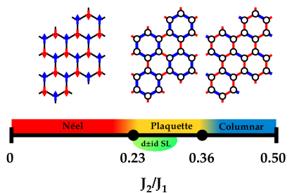
Figure 1: Phase diagram of the spin-$1/2$ $J_{1}\text{-}J_{2}$ Heisenberg model on the honeycomb lattice for $0\leq J_{2}/J_{1}\leq 0.5$ with schematic illustrations of the Néel magnetic order, plaquette, and columnar dimer orders. The full dots indicate quantum phase transitions between Néel and plaquette VBS ($J_{2}/J_{1}\approx 0.23$), and between plaquette and columnar VBS ($J_{2}/J_{1}\approx 0.36$). The region where the $d\pm id$ spin liquid has a competitive energy is marked by the green oval.

II Model and methods

The spin-$1/2$ $J_{1}\text{-}J_{2}$ Heisenberg model is defined by:

$${\cal H}=J_{1}\sum_{\langle i,j\rangle}\mathbf{S}_{i}\cdot\mathbf{S}_{j}+J_{2}\sum_{\langle\langle i,j\rangle\rangle}\mathbf{S}_{i}\cdot\mathbf{S}_{j},$$ (1)

where $\langle i,j\rangle$ and $\langle\langle i,j\rangle\rangle$ denote first- and second-neighbor bonds, respectively (see Fig. 2). The honeycomb lattice has two sites per unit cell and the underlying Bravais lattice has a triangular structure with primitive vectors $\mathbf{a}_{1}=(\sqrt{3},0)$ and $\mathbf{a}_{2}=(\sqrt{3}/2,3/2)$. The two sites in the unit cell are labelled by $A$ and $B$: the former one is placed in the origin of the cell, while the latter one is displaced by the unit vector $\bm{\delta}=(0,1)$ (see Fig. 2). Then, the coordinates of the site $i$ are given by $\mathbf{R}_{i}=\mathbf{R}_{i}^{0}+\eta_{i}\bm{\delta}$, where $\mathbf{R}_{i}^{0}=n_{i}\mathbf{a}_{1}+m_{i}\mathbf{a}_{2}$, $n_{i}$ and $m_{i}$ being integers and the two sites in the unit cell having the same $\mathbf{R}_{i}^{0}$, and $\eta_{i}=0$ or $1$. Note that our choice of primitive vectors is such that the first-neighbor distance is equal to $1$. For our numerical calculations, we take lattice clusters that are defined by $\mathbf{T}_{1}=2L\mathbf{a}_{2}-L\mathbf{a}_{1}$ and $\mathbf{T}_{2}=L\mathbf{a}_{2}+L\mathbf{a}_{1}$, thus consisting of $N_{s}=6L^{2}$ sites (i.e., $3L^{2}$ unit cells with two sites each). Periodic boundary conditions are imposed on the spin model of Eq. (1).

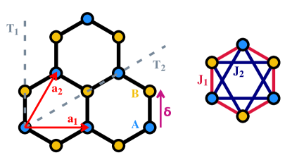
Figure 2: The honeycomb lattice is shown on the left: $\mathbf{a}_{1}$ and $\mathbf{a}_{2}$ are the primitive vectors of the Bravais lattice. $A$ and $B$ denote the two sublattices: $A$-type sites are placed at the origin of the unit cell while $B$-type sites are displaced by $(0,1)$. The dashed lines represent the directions of the vectors $\mathbf{T}_{1}$ and $\mathbf{T}_{2}$ that define the finite lattice clusters used in the calculations. A schematic illustration of the interactions in the $J_{1}\text{-}J_{2}$ Heisenberg model is shown on the right.

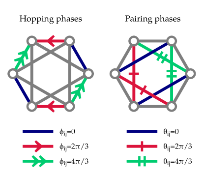
Figure 3: Schematic illustration of the $d\pm id$ spin liquid state. Here, $\phi_{ij}$ and $\theta_{ij}$ are the complex phases of first-neighbor hopping and second-neighbor pairing, respectively. The direction of the arrows ($i\rightarrow j$) indicates the convention of phases for the hopping terms.

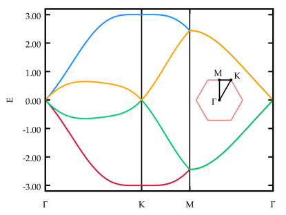
Figure 4: Mean-field spectrum of the gapless $d\pm id$ pairing state. The energy bands are shown along the path $\Gamma\to K\to M\to\Gamma$ in the Brillouin zone (inset). The value of the second-neighbor pairing is $\Delta=0.35t$, which is very close to the optimal value obtained for $J_{2}/J_{1}=0.35$. The bands show Dirac cones located at $\Gamma$ and $K$ points. Note that the two bands are twice degenerate along $M\to\Gamma$.

Our results are obtained using variational wave functions constructed from so-called Gutzwiller-projected fermionic states defined as

$$|\Psi\rangle=\mathcal{P}_{S_{z}^{\rm tot}}\mathcal{J}_{z}\mathcal{P}_{G}|\Phi_{0}\rangle.$$ (2)

Here, $|\Phi_{0}\rangle$ is the ground state of suitable quadratic Hamiltonians for auxiliary spinful fermions $\{c_{i,\uparrow}^{\phantom{\dagger}},c_{i,\downarrow}^{\phantom{\dagger}}\}$ described below. $\mathcal{P}_{G}=\prod_{i}(n_{i,\uparrow}-n_{i,\downarrow})^{2}$ is the Gutzwiller projector that enforces exactly one fermion per site ($n_{i,\sigma}=c_{i,\sigma}^{\dagger}c_{i,\sigma}^{\phantom{\dagger}}$), which is needed in order to obtain a faithful wave function for the Heisenberg model. $\mathcal{P}_{S_{z}^{\rm tot}}$ is the projector on the subspace in which the $z$-component of the total spin is zero. Finally, $\mathcal{J}_{z}$ is the spin-spin Jastrow factor:

$$\mathcal{J}_{z}=\exp\left(-\frac{1}{2}\sum_{i,j}v_{ij}S^{z}_{i}S^{z}_{j}\right),$$ (3)

where the pseudopotential $v_{ij}$ depends on the distance $|\mathbf{R}_{i}-\mathbf{R}_{j}|$ (for a translationally invariant system).

Let us now describe in detail the form of the quadratic Hamiltonians that are used to define $|\Phi_{0}\rangle$. We will mainly consider two options: one for magnetically ordered, the other for nonmagnetic phases. In the first case, we take:

$${\cal H}_{\rm mag}=\sum_{i,j,\sigma}t_{ij}c_{i,\sigma}^{\dagger}c_{j,\sigma}^{\phantom{\dagger}}+h.c.+\sum_{i}h_{i}\left(c_{i,\uparrow}^{\dagger}c_{i,\downarrow}^{\phantom{\dagger}}+c_{i,\downarrow}^{\dagger}c_{i,\uparrow}^{\phantom{\dagger}}\right),$$ (4)

where $t_{ij}$ denotes the hopping amplitude and $h_{i}$ a (fictitious) magnetic field along the $x$ direction, which is taken to have a periodic pattern:

$$h_{j}=h\exp\left[i(\mathbf{Q}\cdot\mathbf{R}_{j}^{0}+\phi_{j})\right],$$ (5)

where $\mathbf{Q}$ is the wave vector that fixes the periodicity, and $\phi_{j}$ is a sublattice-dependent phase shift. In this work, we consider the antiferromagnetic Néel phase with $\mathbf{Q}=(0,0)$ and $\phi_{j}=\eta_{j}\pi$ (i.e., $\phi_{j}=0$ for $j\in A$ and $\phi_{j}=\pi$ for $j\in B$), and a collinear phase with $\mathbf{Q}=(0,2\pi/3)$ and $\phi_{i}=0$. Within this kind of magnetically ordered states, it is very important to take into account the spin-spin Jastrow factor in order to introduce transverse spin fluctuations (i.e., spin waves) Manousakis1991 . We mention in passing that the case $t_{ij}=0$ reduces to a “bosonic” (pure Jastrow) state, which has been used by Di Ciolo et al. for this model Ciolo2014 . Interestingly, we find that a nonzero uniform first-neighbor hopping does provide an energy gain with respect to this “bosonic” case. This situation is similar to the triangular-lattice antiferromagnet, where a hopping term with Dirac spectrum was also found to result in a substantial energy gain Iqbal2016 .

In contrast, nonmagnetic phases, such as spin liquids and VBS, can be described by taking:

$${\cal H}_{\rm sl} = \sum_{i,j,\sigma}t_{ij}c_{i,\sigma}^{\dagger}c_{j,\sigma}^{\phantom{\dagger}}+\sum_{ij}\Delta_{ij}c_{i,\downarrow}^{\phantom{\dagger}}c_{j,\uparrow}^{\phantom{\dagger}}+h.c.$$ (6)

$$+ \sum_{i,\sigma}\mu_{i}c_{i,\sigma}^{\dagger}c_{i,\sigma}^{\phantom{\dagger}}+\sum_{i}\zeta_{i}c_{i,\downarrow}^{\phantom{\dagger}}c_{i,\uparrow}^{\phantom{\dagger}}+h.c.,$$

where, in addition to the hopping, one introduces singlet pairing terms, $\zeta_{i}$ and $\Delta_{ij}=\Delta_{ji}$, as well as a chemical potential $\mu_{i}$. Within this framework, a classification of distinct spin-liquid phases can be obtained through the so-called projective symmetry group (PSG) analysis Wen2002 ; Bieri2016 . From a variational perspective, the PSG provides a recipe for constructing symmetric spin-liquid wave functions through specific Ansätze for the Hamiltonian (6). The simplest Ansatz is given by a first neighbor hopping ($t_{ij}=t$) and no pairing terms ($\Delta_{ij}=\zeta_{i}=0$). This is the uniform resonating valence bond (uRVB) state, which is a $U(1)$ state with Dirac cones at the corners of the hexagonal Brillouin zone. By performing a PSG classification, Lu and Ran Lu2011 found $24$ symmetric $Z_{2}$ spin liquids that are continuously connected to this uRVB (i.e., that can be obtained from uRVB by adding further hopping and/or pairing terms). Among those states, the presence of the gapped SPS was emphasized. The SPS Ansatz is characterized by a uniform first-neighbor hopping $t$ and a complex second-neighbor pairing with opposite phases on $A$-$A$ and $B$-$B$ links, i.e., ${\Delta_{ij}^{AA}=\Delta e^{i\theta}}$ and ${\Delta_{ij}^{BB}=\Delta e^{-i\theta}}$. Such a state is always gapped if ${\Delta\neq 0}$ and ${\theta\neq\pi/2}$. In principle, the PSG classification also allows an on-site pairing with opposite phases on the two sublattices, i.e., ${\zeta_{i}^{A}=\zeta e^{i\phi}}$, ${\zeta_{i}^{B}=\zeta e^{-i\phi}}$. In agreement with previous studies Clark2011 ; Gong2013 , we find that the SPS Ansatz has a lower variational energy than the uRVB state for $J_{2}/J_{1}\gtrsim 0.25$. The actual value of $\theta$ can be set to zero since the variational energy does not change appreciably for $\theta\lesssim\pi/4$. However, here we find another gapless spin liquid (i.e., number $18$ in Table I of Ref. Lu2011 ) that has an even lower energy than the SPS wave function and represents the best $Z_{2}$ state among those classified within the fermionic PSG. We adopt a natural gauge in which this spin liquid Ansatz has first-neighbor hopping $t_{ij}=te^{i\phi_{ij}}$ and second-neighbor pairing $\Delta_{ij}=\Delta e^{i\theta_{ij}}$ with complex phases as given in Fig. 3, a convention that differs from the original PSG solution of Ref. Lu2011 . Since $\Delta_{ij}$ has a $d_{x^{2}-y^{2}}+id_{xy}$ phase winding on the triangular lattice of $A$ sites and $d_{x^{2}-y^{2}}-id_{xy}$ on the $B$ sublattice, we call this new state $d\pm id$. For $\Delta=0$, the $d\pm id$ state reduces to uRVB, while for $t=0$, it is two copies of the quadratic band touching state that has been discussed in Ref. Mishmash2013 for the triangular lattice. For finite $\Delta$, the fermionic mean-field energy bands show Dirac nodes at the center and at the corners of the Brillouin zone (see Fig. 4). Note that, despite the presence of complex hopping and pairing terms, both the SPS and the $d\pm id$ states do not break time-reversal symmetry (or any other lattice symmetry) once the wave function is Gutzwiller-projected to the physical spin Hilbert space (see Appendix A for its projective symmetries). Beyond fully symmetric phases, we also looked for potential chiral spin liquids as outlined in Ref. Bieri2016 . However, we do not find any indication for such ground states in the present model.

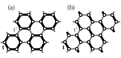
Figure 5: Patterns of the first-neighbor hoppings in the quadratic Hamiltonian (6) as found in the plaquette VBS (a) and in the columnar VBS (b).

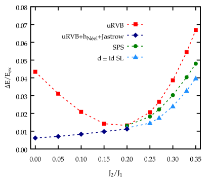
Figure 6: Accuracy of the variational energy for different wave functions on the $24$-site cluster. Here, $\Delta E$ is the difference between the variational ($E_{var}$) and the exact ground-state energy ($E_{ex}$).

Using the Hamiltonian of Eq. (6), we can also construct wave functions with VBS order. This can be achieved by allowing a translation and/or rotation symmetry breaking in the hopping $t_{ij}$ and/or in the pairing $\Delta_{ij}$ parameters. Here, we consider two possibilities which are motivated by recent DMRG results Zhu2013 ; Gong2013 ; Ganesh2013b . These are obtained by considering two different first-neighbor hoppings $t$ and $t^{\prime}$, forming “strong” and “weak” plaquettes or columnar dimers, see Fig. 5. In both cases, a remarkable improvement in variational energy is achieved by adding a (uniform) second-neighbor pairing with $d\pm id$ symmetry, as well as including the corresponding complex phases for the dimerized first-neighbor hoppings (Fig. 3). These are rare examples of clear VBS instabilities in frustrated two-dimensional Heisenberg models using Peierls-type mean-field parameters in Gutzwiller-projected wave functions (see, e.g., Ref. Iqbal2012 ).

Finally, we would like to emphasize that, in order to calculate observables (e.g., the variational energy, or any correlation function) in the state of Eq. (2), Monte Carlo sampling is needed, since an analytic treatment is not possible in two spatial dimensions. The optimal variational parameters (including the ones defining the quadratic Hamiltonian and the Jastrow pseudo potential), for each value of the ratio $J_{2}/J_{1}$, can be obtained using the stochastic reconfiguration technique Sorella2005 .

III Results

In the following, we show the numerical results obtained by the variational approach described in the previous section.

III.1 Accuracy of the wave functions

Let us first discuss the accuracy of the optimized variational energy for various states on a small lattice cluster with $24$ sites (i.e., $L=2$) for which exact diagonalization is available. In Fig. 6, we present the results for the uRVB state (with only first-neighbor hopping), the Néel state (also including the fictitious magnetic field $h_{i}$ and the spin-spin Jastrow factor), the SPS Ansatz (with second-neighbor pairing and $\theta=0$), and the $d\pm id$ state. First of all, starting from the unfrustrated limit with $J_{2}=0$, the accuracy of the uRVB state clearly improves until $J_{2}/J_{1}\approx 0.2$. Then the energy rapidly deteriorates when $J_{2}/J_{1}$ is further increased. For $J_{2}/J_{1}\lesssim 0.2$, the best variational state is given by including Néel order with $\mathbf{Q}=(0,0)$ and $\phi_{i}=\eta_{i}\pi$. In this regime, the strength of the magnetic field $h$ in Eq. (5) decreases as $J_{2}/J_{1}$ increases, and it goes to zero for $J_{2}/J_{1}\gtrsim 0.2$. When $h=0$, only a marginal energy gain with respect to the uRVB state is obtained, due to a (small) spin-spin Jastrow factor. For this reason, the results for the Néel state are not reported for $J_{2}/J_{1}>0.2$. In contrast, an energy gain is found in this regime by allowing a pairing term in Eq. (6). Here, both the SPS and the $d\pm id$ Ansätze give a lower variational energy than the simple uRVB. We emphasize that the $d\pm id$ wave function represents the best fermionic state among the $24$ $Z_{2}$ spin liquids listed in Ref. Lu2011 . On the small cluster considered, there is no significant energy gain by allowing VBS order on top of the $d\pm id$ state for $J_{2}/J_{1}\lesssim 0.35$.

Figure 7: Finite-size scaling of the squared magnetization $m^{2}$, Eq. (7), for different values of $J_{2}/J_{1}$. For $J_{2}=0$ the optimal value of the fictitious magnetic field is $h/t\approx 0.32$.

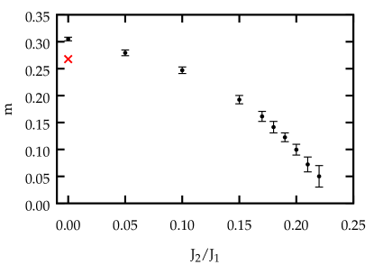
Figure 8: Thermodynamic limit of the magnetization $m$ as a function of $J_{2}/J_{1}$. The result from quantum Monte Carlo of Ref. Castro2006 for $J_{2}=0$ is shown for comparison (red cross). The classical value is $m=0.5$.

III.2 The Néel phase

In order to draw the ground-state phase diagram, we focus on the Néel phase and perform a finite-size scaling of the magnetization, which is obtained from the expectation value of the spin-spin correlation at the maximal distance

$$m^{2}=\lim_{|i-j|\to\infty}\langle\mathbf{S}_{i}\cdot\mathbf{S}_{j}\rangle,$$ (7)

in the variational state $|\Psi\rangle$. The results for $0\leq J_{2}/J_{1}\leq 0.22$ are reported in Fig. 7 for $L$ ranging from $6$ to $10$ (i.e., up to $600$ sites). The thermodynamic extrapolation of the magnetization $m$ is shown in Fig. 8. The expected $1/L$ corrections are correctly reproduced by the spin-spin Jastrow factor, which is able to introduce the relevant low-energy fluctuations on top of the classical order parameter that is generated by the magnetic field $h$ of Eq. (5). The thermodynamic value of the staggered magnetization vanishes for $J_{2}/J_{1}\approx 0.23$ (see also the discussion in Sec. IV), in good agreement with previous DMRG calculations Zhu2013 ; Gong2013 ; Ganesh2013b . We remark that the value $J_{2}/J_{1}\approx 0.23$ is larger than the one obtained in the classical limit (i.e., $J_{2}/J_{1}=1/6$), indicating that quantum fluctuations favor collinear magnetic order over generic coplanar spirals (which represent the classical ground state for $J_{2}/J_{1}>1/6$). Comparison with exact quantum Monte Carlo calculations, which are only possible in the unfrustrated case $J_{2}=0$ Castro2006 , further substantiates the accuracy of the Néel wave function on large systems, see Fig. 8. Even though a direct inspection of our numerical results cannot exclude a first-order transition at $J_{2}/J_{1}\approx 0.23$, a detailed finite-size scaling analysis based on data collapse suggests that the transition between the Néel and the nonmagnetic phase is continuous (see below).

III.3 The nonmagnetic phase

Increasing the ratio $J_{2}/J_{1}$, the Néel order melts and the natural expectation is that a nonmagnetic phase is stabilized by quantum fluctuations. Nonetheless, we cannot exclude that magnetic states with incommensurate spirals are favored instead, as it happens in the classical limit for $J_{2}/J_{1}>1/6$. In any numerical calculation that considers finite clusters, it is very difficult to assess states with large periodicity or with pitch vectors that are not allowed by the finite cluster geometry. Therefore, we will not consider the possibility of incommensurate spiral orders here, and we restrict ourselves to states with collinear order, i.e., the one with $\mathbf{Q}=(0,2\pi/3)$ and $\phi_{i}=0$. This restriction is justified by recent variational Monte Carlo results showing that collinear (or short-period spirals) may prevail over generic states with long periodicity Ciolo2014 . As far as the nonmagnetic states are concerned, we consider the ones that can be constructed with the help of the Hamiltonian (6). For these cases, we do not include the spin-spin Jastrow factor (3), since this term would break SU(2) spin rotation symmetry (in any case, the inclusion of a Jastrow factor only leads to minor energy gains).

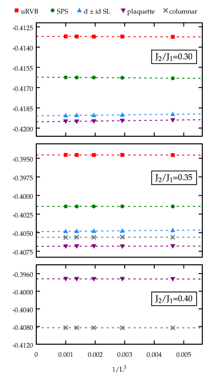
Figure 9: Finite-size scaling analysis of the variational energy of different wave functions for $J_{2}/J_{1}=0.3$, $0.35$, and $0.4$. Statistical errors are smaller than the symbol size. The uRVB, SPS, and $d\pm id$ states are reported only for $J_{2}/J_{1}=0.3$ and $0.35$; for $J_{2}/J_{1}=0.4$, their energies are much higher than the ones of plaquette and columnar dimer VBS states. The dashed lines are the fitting functions used for the extrapolation to the thermodynamic limit. For the $d\pm id$ state, the optimal values of the parameters are $\Delta/t\approx 0.31$ and $\Delta/t\approx 0.36$ for $J_{2}/J_{1}=0.3$ and $0.35$, respectively. For the plaquette state the parameters range from $\Delta/t\approx 0.31$ and $t^{\prime}/t\approx 0.90$ for $J_{2}/J_{1}=0.3$ to $\Delta/t\approx 0.38$ and $t^{\prime}/t\approx 0.62$ for $J_{2}/J_{1}=0.4$. Finally, for the columnar state we get $\Delta/t\approx 0.34$ ($\Delta/t\approx 0.37$) and $t^{\prime}/t\approx 0.45$ ($t^{\prime}/t\approx 0.20$) for $J_{2}/J_{1}=0.35$ ($J_{2}/J_{1}=0.4$).

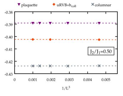
Figure 10: Finite-size scaling analysis of the variational energy of VBS and collinear magnetic states at $J_{2}/J_{1}=0.5$. The optimal values for the plaquette state are $\Delta/t\approx 0.40$ and $t^{\prime}/t\approx 0.20$. For the columnar state $t^{\prime}/t$ is essentially zero, while $\Delta/t\approx 0.37$. The fictitious magnetic field of the collinear state has optimal value $h/t\approx 0.98$.

In Fig. 9, we report the finite-size scaling of the energies for $J_{2}/J_{1}=0.3$, $0.35$, and $0.4$. Various variational wave functions are reported, since the uRVB is unstable when adding pairing terms or allowing a translation symmetry breaking in the quadratic Hamiltonian. First of all, the SPS Ansatz gives a size-consistent improvement with respect to the uRVB state in both cases. Our calculations are shown for $\theta=0$. In addition to the second-neighbor pairing, the symmetry-allowed nonzero on-site pairing leads to a gapless mean-field spectrum, spoiling the gapped nature of the SPS Ansatz. However, this variational freedom does not give an appreciable energy gain for the values of $J_{2}/J_{1}$ considered here. The best spin-liquid wave function, among the $24$ possibilities listed in Ref. Lu2011 , is the $d\pm id$ state discussed in Sec. II. But most strikingly, the lowest-energy state in this regime has plaquette VBS order, where the first-neighbor hoppings exhibit the pattern shown in Fig. 5(a). Here, the presence of a second-neighbor pairing with $d\pm id$ symmetry gives a significant improvement in the variational energy, but the stabilization of a plaquette state is already observed using first-neighbor hopping only. Its energy gain with respect to the uniform $d\pm id$ Ansatz clearly increases with increasing $J_{2}/J_{1}$, being approximately $5\times 10^{-4}J_{1}$ for $J_{2}/J_{1}=0.3$ and $2\times 10^{-3}J_{1}$ for $J_{2}/J_{1}=0.35$ (see Fig. 9).

Further increasing $J_{2}/J_{1}$, a different VBS with columnar order wins over the plaquette VBS, see Fig. 9. The corresponding pattern of first-neighbor hoppings is shown in Fig. 5(b). Again, a second-neighbor $d\pm id$ pairing gives a substantial energy gain, allowing us to obtain a stable optimization of the columnar order. The fact that both columnar and plaquette states can be stabilized, even when their respective energy is higher than the one of the competitor, strongly suggests that the transition between these two VBS phases is first order. Based on the calculation of variational energies on relatively large clusters, our estimation of the transition point is $J_{2}/J_{1}\approx 0.36$ (in remarkably good agreement with DMRG Zhu2013 ; Ganesh2013b ).

Finally, we briefly discuss the possible emergence of magnetic order close to $J_{2}/J_{1}=0.5$. Unfortunately, the pitch vector of the relevant magnetic state that is found at the classical and semiclassical levels varies continuously with $J_{2}/J_{1}$ Fouet2001 ; Mulder2010 . This fact makes it impossible to determine the best spiral state on finite clusters. However, for $J_{2}/J_{1}=0.5$, the classical state that is selected by quantum fluctuations is relatively simple, having collinear order. More specifically, it has spins that are antiferromagnetically aligned on two out of the three first-neighbor directions, and ferromagnetically aligned on the third direction. There are three inequivalent possibilities for this ordering (corresponding to the choice of the ferromagnetic bond) and, therefore, this state breaks rotation symmetry (similar to the $J_{1}\text{-}J_{2}$ model on the square lattice for $J_{2}/J_{1}>0.5$ Chandra1990 ). In the following, we compare the VBS and the collinear magnetic state for $J_{2}/J_{1}=0.45$ and $0.5$. We take the best VBS Ansatz, which is given by the columnar state (including the $d\pm id$ pairing), and a magnetically ordered wave function, which is constructed using Eq. (4) with $\mathbf{Q}=(0,2\pi/3)$ and $\phi_{i}=0$. The results of the finite-size scaling of the energies are shown in Fig. 10 for $J_{2}/J_{1}=0.5$ (similar results are obtained for $J_{2}/J_{1}=0.45$). In this regime, the VBS Ansatz overcomes the collinear state with a remarkable energy gain. Therefore, we can safely affirm that, for $0.36\lesssim J_{2}/J_{1}\leq 0.5$, the best variational wave function exhibits VBS order. These results are in agreement with previous studies Clark2011 ; Ganesh2013b , which detected signatures of rotation-symmetry breaking, and suggested the existence of a dimerized phase for large values of $J_{2}/J_{1}$.

III.4 Néel to VBS transition: finite-size scaling analysis

In this last section, we briefly discuss the possibility for the Néel to VBS transition to be an example of the so-called deconfined quantum criticality Senthil2004a ; Senthil2004b as suggested by Ganesh et al. Ganesh2013a ; Ganesh2013b . We compute both the magnetization [see Eq. (7)] and the VBS order parameter:

$$\psi=\frac{1}{N}\sum_{i\in A}\langle D_{i}\rangle e^{-i\frac{2\pi}{3}(n_{i}-m_{i})},$$ (8)

where

$$D_{i}=S^{z}_{i}S^{z}_{i+x}+S^{z}_{i}S^{z}_{i+y}e^{i\frac{2\pi}{3}}+S^{z}_{i}S^{z}_{i+z}e^{-i\frac{2\pi}{3}}.$$ (9)

Here, site $i$ has coordinates $\mathbf{R}_{i}=n_{i}\mathbf{a}_{1}+m_{i}\mathbf{a}_{2}$ (belonging to sublattice $A$), while sites $i+x$, $i+y$, and $i+z$ have coordinates $\mathbf{R}_{i}-\mathbf{a}_{2}+\bm{\delta}$, $\mathbf{R}_{i}+\mathbf{a}_{1}-\mathbf{a}_{2}+\bm{\delta}$, and $\mathbf{R}_{i}+\bm{\delta}$, respectively Pujari2015 . Note that, since the variational wave function explicitly breaks translation symmetry, the order parameter (and not its square) can be directly assessed in the numerical calculation. For continuous transitions, we have:

$$m^{2}L^{1+\eta_{m}} = F_{m}\left[\left(\frac{J_{2}-J_{cm}}{J_{cm}}\right)L^{1/\nu_{m}}\right],$$ (10)

$$|\psi|^{2}L^{1+\eta_{p}} = F_{p}\left[\left(\frac{J_{2}-J_{cp}}{J_{cp}}\right)L^{1/\nu_{p}}\right],$$ (11)

where $\nu_{m}$ ($\nu_{p}$) is the exponent for the magnetic (plaquette) correlation length, $\eta_{m}$ ($\eta_{p}$) is the exponent for this correlation function at criticality, and $J_{cm}$ and $J_{cp}$ are the values of $J_{2}$ at the transition points. Finally, $F_{m}$ and $F_{p}$ are suitable scaling functions. In the case of deconfined criticality, we must have $J_{cm}=J_{cp}$ and $\nu_{m}=\nu_{p}$, while the exponents are different, i.e., $\eta_{m}\neq\eta_{p}$. The results for the magnetization $m^{2}$ and for the plaquette order $|\psi|^{2}$ are reported in Fig. 11. Performing two separate fitting procedures based on a Bayesian statistical analysis Harada , we get $J_{cm}=0.234(1)$, $\nu_{m}=0.664(1)$, $\eta_{m}=0.837(1)$ for the magnetization, and $J_{cp}=0.224(1)$, $\nu_{p}=1.077(1)$, $\eta_{p}=0.799(1)$ for the plaquette order. These fitting procedures give a remarkably good collapse of the two curves. Note that the evaluations of the critical points are in very good agreement, and also the values of $\eta_{s}$ and $\eta_{p}$ may be compatible with the prediction of the theory Kaul2013 . However, the values of the exponents $\nu_{m}$ and $\nu_{p}$ are quite different, with an anomalously large value obtained for $|\psi|^{2}$. In fact, when attempting to fit both curves with the same $\nu$, a much worse result is obtained (not shown) and the data collapsing procedure fails in a large part of the magnetization curve.

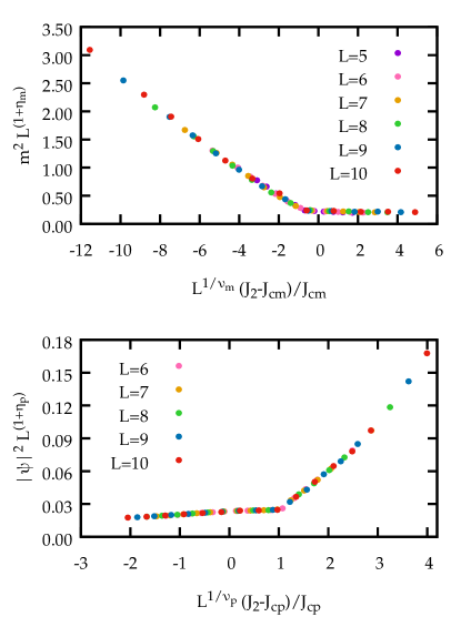
Figure 11: Finite-size scaling collapse of the data of the antiferromagnetic (above) and plaquette (below) order parameters.

When analyzing these scaling results, one must keep in mind that they are obtained within a variational approach, which may miss subtle details of the final phase diagram. Therefore, it can be very difficult to detect the existence of a deconfined quantum criticality. Nevertheless, it is striking that the two transitions look continuous with critical values $J_{c}$ that are extremely close to each other. The failure to obtain a good collapse with a single exponent $\nu$ could be due to the approximate nature of the variational wave function, which may not be particularly accurate in the VBS region (see Fig. 6).

IV Conclusions

In conclusion, we have employed variational wave functions and quantum Monte Carlo methods to study the frustrated $J_{1}\text{-}J_{2}$ Heisenberg model on the honeycomb lattice. We find that quantum fluctuations enlarge the region of stability of the collinear Néel phase with respect to the classical model, up to $J_{2}/J_{1}\approx 0.23$. Further increasing $J_{2}/J_{1}$, a plaquette VBS order is stabilized, even though a gapless $Z_{2}$ spin liquid (dubbed $d\pm id$) represents a state with highly competitive variational energy, especially in the proximity of the phase transition. We expect that this interesting new spin liquid can possibly be favored by farther-range couplings or by ring-exchange terms. At $J_{2}/J_{1}\approx 0.36$, another VBS state with columnar order becomes energetically favored. Our results are in excellent agreement with recent DMRG calculations Zhu2013 ; Gong2013 ; Ganesh2013b .

Regarding the nature of the Néel to VBS transition, we hope that the promising results obtained by our approach will give a new impetus to examine the topic of a deconfined quantum critical point in the frustrated Heisenberg model on the honeycomb lattice.

Appendix A PSG of the $d\pm id$ spin liquid

In this appendix, we shortly discuss the projective symmetry group Wen2002 ; Bieri2016 and some physical properties of the competitive $d\pm id$ state discussed in this paper. For this purpose, we introduce a different formulation of the Hamiltonian of Eq. (6), dropping the on-site terms which are not relevant for the present discussion:

$${\cal H}_{\rm sl}=\sum_{i,j}\psi^{\dagger}_{i}u_{ij}\psi_{j}=\sum_{i,j}(c_{i,\uparrow}^{\dagger},c_{i,\downarrow}^{\phantom{\dagger}})\begin{pmatrix}t_{ij}&\Delta^{*}_{ij}\\ \Delta_{ij}&-t_{ij}^{*}\\ \end{pmatrix}\begin{pmatrix}c_{j,\uparrow}\\ c_{j,\downarrow}^{\dagger}\\ \end{pmatrix}.$$ (12)

A spin liquid Ansatz $u_{ij}$ is invariant under the combined effect of a lattice symmetry transformation ($\mathcal{O}$) and the corresponding gauge transformation ($g_{\mathcal{O}}$), namely

$$u_{ij}=g_{\mathcal{O}}(i)u_{\mathcal{O}^{-1}(i)\mathcal{O}^{-1}(j)}g_{\mathcal{O}}^{\dagger}(j).$$ (13)

The $d\pm id$ spin-liquid state is classified as No. 18 in Table I of Ref. Lu2011 . In the gauge employed in that paper, the quadratic mean-field Hamiltonian has a large cell (i.e., 6 sites). Here, we use a more natural gauge where the unit cell of the honeycomb lattice is not enlarged. In our gauge, both first-neighbor hopping phases and second-neighbor pairing phases undergo a $l=2$ phase winding as shown in Fig. 3. As a tradeoff for the simplicity of the Ansatz, the projective representation of symmetries is slightly more involved in this gauge.

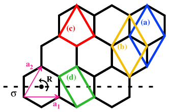
Figure 12: Symmetry generators of the point group of the honeycomb lattice ($\sigma$ and $R$). As an example, we show the loops for which we computed the $SU(2)$ flux: (a) parallelogram-shaped (sublattice A), (b) parallelogram-shaped (sublattice B), (c) diamond and (d) rectangular plaquettes.

More explicitly, in our gauge we have trivial representations of lattice translations along $\mathbf{a}_{1}$ and $\mathbf{a}_{2}$, namely $g_{1}=g_{2}=\mathbbm{1}_{2}$. The projective representation of the point group symmetries, i.e. the mirror reflection $\sigma$ and the $6$-fold rotation $R$ (see Fig. 12), is the following:

$$g_{\sigma}(s)=\mathbbm{1}_{2},$$ (14)

$$g_{R}(s)=(-)^{s}i\sigma_{1}e^{(1-2s)\frac{\pi}{3}i\sigma_{3}},$$ (15)

where $s=0,1$ is the sublattice index. Finally, for the time reversal $T$, we have

$$g_{T}(s)=(-)^{s}i\sigma_{3}.$$ (16)

For example, Eq. (16) implies that complex hopping terms between sites of different sublattices, and complex pairing terms between sites of the same sublattice are time-reversal invariant Bieri2016 . The gauge transformation that relates our gauge for the $d\pm id$ state with the one used in Ref. Lu2011 (No. 18 in Table I) is given by:

$$g(j)=(-i\sigma_{3})^{s}\exp\left[{i\frac{\pi}{12}\sigma_{3}}\right]\exp\left[{-i\frac{2\pi}{3}(n_{j}-m_{j})\sigma_{3}}\right].$$ (17)

In our gauge the Ansatz matrix reads

$$u_{ij}=\begin{cases}t\sigma_{3}\exp\left[i\phi_{ij}\sigma_{3}\right],\ (i,j)\mbox{ first-neighbor}\\ \Delta\sigma_{1}\exp\left[i\theta_{ij}\sigma_{3}\right],\ (i,j)\mbox{ second-neighbor},\end{cases}$$ (18)

where the phases $\phi_{ij}$ and $\theta_{ij}$ are the ones of Fig. 3.

To conclude, let us discuss the gauge-invariant fluxes of the $d\pm id$ state on the honeycomb lattice. For any lattice loop $\mathcal{C}$ with base site $j$, we can define the SU(2) flux

$$P_{j}=\prod_{\mathcal{C}}u_{kl}=u_{jj_{2}}u_{j_{2}j_{3}}\cdots u_{j_{p}j}.$$ (19)

where $p$ is the number of sites in the loop. The trace of the $2\times 2$ matrix $P_{j}$ is independent of the base site $j$ Bieri2016

$$\operatorname{Tr}P_{j}=\begin{cases}2\rho\cos(\theta),\ p\mbox{ even}\\ 2i\rho\sin(\theta),\ p\mbox{ odd},\end{cases}$$ (20)

and the angle $\theta$ is the gauge-invariant quantity that characterizes the SU(2) gauge flux.

For the $d\pm id$ Ansatz, pure first-neighbor loops have trivial fluxes ($\theta=0$), since the first-neighbor hopping is gauge equivalent to the uRVB state. The second-neighbor pairings, however, have nontrivial SU(2) flux with $\theta=\pm 2\pi/3$ through the parallelogram-shaped plaquettes of the triangular sublattices $A$ [Fig. 12, loop (a)] and $B$ [Fig. 12, loop (b)]. Odd-site loops do not contain nontrivial flux since the state is time-reversal invariant. As far as loops made from two first- and two second-neighbor links are concerned, we can either have a diamond $J_{1}J_{1}J_{2}J_{2}$ [Fig. 12, loop (c)] or a rectangular $J_{1}J_{2}J_{1}J_{2}$ [Fig. 12, loop (d)] plaquette. In the $d\pm id$ state, the trace of flux through the diamond plaquettes is trivial, while it gives $\theta=\pi$ through the rectangular plaquettes. These gauge-invariant fluxes are related to expectation values of certain multiple-spin operators Bieri2016 .

References

- (1) See for example, C. Lacroix, P. Mendels, and F. Mila, Introduction to Frustrated Magnetism: Materials, Experiments, Theory, Vol. 164 (Springer, New York, 2011).
- (2) H.-C. Jiang, H. Yao, and L. Balents, Phys. Rev. B86, 024424 (2012).
- (3) W.-J. Hu, F. Becca, A. Parola, and S. Sorella, Phys. Rev. B88, 060402 (2013).
- (4) L. Wang, D. Poilblanc, Z.-C. Gu, X.-G. Wen, and F. Verstraete, Phys. Rev. Lett. 111, 037202 (2013).
- (5) S.-S. Gong, W. Zhu, D. N. Sheng, O. I. Motrunich, and M. P. A. Fisher, Phys. Rev. Lett. 113, 027201 (2014).
- (6) D. Poilblanc and M. Mambrini, arXiv:1702.05950.
- (7) R. V. Mishmash, J. R. Garrison, S. Bieri, and C. Xu, Phys. Rev. Lett. 111, 157203 (2013).
- (8) R. Kaneko, S. Morita, and M. Imada, J. Phys. Soc. Japan 83, 093707 (2014).
- (9) Z. Zhu and S. R. White, Phys. Rev. B92, 041105 (2015).
- (10) W.-J. Hu, S.-S. Gong, W. Zhu, and D. N. Sheng, Phys. Rev. B92, 140403 (2015).
- (11) Y. Iqbal, W.-J. Hu, R. Thomale, D. Poilblanc, and F. Becca, Phys. Rev. B93, 144411 (2016).
- (12) S. Yan, D. A. Huse, and S. R. White, Science 332, 1173 (2011).
- (13) S. Depenbrock, I. P. McCulloch, and U. Schollwöck, Phys. Rev. Lett. 109, 067201 (2012).
- (14) Y. Iqbal, F. Becca, S. Sorella, and D. Poilblanc, Phys. Rev. B87, 060405 (2013).
- (15) Y.-C. He, M.P. Zaletel, M. Oshikawa, F. Pollmann, arXiv:1611.06238.
- (16) H.J. Liao, Z.Y. Xie, J. Chen, Z.Y. Liu, H. D. Xie, R. Z. Huang, B. Normand, and T. Xiang, Phys. Rev. Lett. 118, 137202 (2017).
- (17) E. H. Lieb, T. Schultz, and D. J. Mattis, Ann. Phys. (N.Y.) 16, 407 (1961).
- (18) I. Affleck, Phys. Rev. B37, 5186 (1988).
- (19) M. Oshikawa, Phys. Rev. Lett. 84, 1535 (2000).
- (20) G. Misguich, C. Lhuillier, M. Mambrini, and P. Sindzingre, Eur. Phys. J. B 26, 167 (2002).
- (21) M. B. Hastings, Phys. Rev. B69, 104431 (2004).
- (22) E. Rastelli, A. Tassi, and L. Reatto, Physica B 97, 1 (1979)
- (23) J.-B. Fouet, P. Sindzingre, and C. Lhuillier, Eur. Phys. J. B 20, 241 (2001).
- (24) A. Mulder, R. Ganesh, L. Capriotti, and A. Paramekanti, Phys. Rev. B81, 214419 (2010).
- (25) F. Wang, Phys. Rev. B82, 024419 (2010).
- (26) Y.M. Lu and Y. Ran, Phys. Rev. B84, 024420 (2011).
- (27) B. K. Clark, D. A. Abanin, and S. L. Sondhi, Phys. Rev. Lett. 107, 087204 (2011).
- (28) F. Mezzacapo and M. Boninsegni, Phys. Rev. B85, 060402 (2012).
- (29) A. Di Ciolo, J. Carrasquilla, F. Becca, M. Rigol, and V. Galitski, Phys. Rev. B89, 094413 (2014).
- (30) R. F. Bishop, P. H. Y. Li, and C. E. Campbell, J. Phys.: Condens. Matter 25, 306002 (2013).
- (31) J. Reuther, D. A. Abanin, and R. Thomale, Phys. Rev. B84, 014417 (2011).
- (32) J. Oitmaa and R. R. P. Singh, Phys. Rev. B84, 094424 (2011).
- (33) H. Mosadeq, F. Shabazi, and S. A. Jafary, J. Phys.: Condens. Matter 23, 226006 (2011).
- (34) A. F. Albuquerque, D. Schwandt, B. Hetenyi, S. Capponi, M. Mambrini, and A. M. Läuchli, Phys. Rev. B84, 024406 (2011).
- (35) Z. Zhu, D. A. Huse, and S. R. White, Phys. Rev. Lett. 110, 127205 (2013).
- (36) S.-S. Gong, D.N. Sheng, O. I. Motrunich, and M. P. A. Fisher, Phys. Rev. B88, 165138 (2013).
- (37) R. Ganesh, S. Nishimoto, and J. van den Brink, Phys. Rev. B87, 054413 (2013).
- (38) R. Ganesh, J. van den Brink, and S. Nishimoto, Phys. Rev. Lett. 110, 127203 (2013).
- (39) R. Flint and P. A. Lee, Phys. Rev. Lett. 111, 217201 (2013).
- (40) Z. Y. Meng, T. C. Lang, S. Wessel, F. F. Assaad, A. Muramatsu, Nature 464, 847 (2010).
- (41) S. Sorella, Y. Otsuka, and S. Yunoki, Sci. Rep. 2, 992 (2012).
- (42) E. Manousakis, Rev. Mod. Phys. 63, 1 (1991).
- (43) X.-G. Wen, Phys. Rev. B65, 165113 (2002).
- (44) S. Bieri, C. Lhuillier, and L. Messio, Phys. Rev. B93, 094437 (2016).
- (45) Y. Iqbal, F. Becca, and D. Poilblanc, New J. Phys. 14, 115031 (2012).
- (46) S. Sorella, Phys. Rev. B71, 241103 (2005).
- (47) E. V. Castro, N. M. R. Peres, K. S. D. Beach, and A. W. Sandvik, Phys. Rev. B73, 054422 (2006).
- (48) P. Chandra, P. Coleman, and A. I. Larkin, Phys. Rev. Lett. 64, 88 (1990).
- (49) T. Senthil, A. Vishwanath, L. Balents, S. Sachdev, and M. P. A. Fisher, Science 303, 1490 (2004).
- (50) T. Senthil, L. Balents, S. Sachdev, A. Vishwanath, and M. P. A. Fisher, Phys. Rev. B70, 144407 (2004).
- (51) S. Pujari, F. Alet, and K. Damle Phys. Rev. B91, 104411 (2015).
- (52) K. Harada, Phys. Rev. E84, 056704 (2011); Phys. Rev. E92, 012106 (2015).
- (53) R. K. Kaul, R. G. Melko, and A. W. Sandvik, Annu. Rev. Con. Mat. Phys. 4, 179 (2013).