A computer algebra system for R: Macaulay2 and the m2r package

Abstract

Algebraic methods have a long history in statistics. The most prominent manifestation of modern algebra in statistics can be seen in the field of algebraic statistics, which brings tools from commutative algebra and algebraic geometry to bear on statistical problems. Now over two decades old, algebraic statistics has applications in a wide range of theoretical and applied statistical domains. Nevertheless, algebraic statistical methods are still not mainstream, mostly due to a lack of easy off-the-shelf implementations. In this article we debut m2r, an R package that connects R to Macaulay2 through a persistent back-end socket connection running locally or on a cloud server. Topics range from basic use of m2r to applications and design philosophy.

1 Introduction

Algebra, a branch of mathematics concerned with abstraction, structure, and symmetry, has a long history of applications in statistics. For example, Pearson’s early work on method of moments estimation in mixture models ultimately involved systems of polynomial equations that he painstakingly and remarkably solved by hand (Pearson, 1894; Améndola et al., 2016). Fisher’s work in design was strongly algebraic and combinatorial, focusing on topics such as Latin squares (Fisher, 1934). Invariance and equivariance continue to form a major pillar of mathematical statistics through the lens of location-scale families (Pitman, 1939; Bondesson, 1983; Lehmann and Romano, 2005).

Apart from the obvious applications of linear algebra, the most visible manifestations of modern algebra in statistics are found in the young field of algebraic statistics. Algebraic statistics is defined broadly as the application of commutative algebra and algebraic geometry to statistical problems, generally understood to include applications of other mathematical fields that have substantial overlap with commutative algebra and algebraic geometry, such as combinatorics, polyhedral geometry, graph theory, and others (Drton et al., 2009; Sturmfels, 1996). Now a quarter century old, algebraic statistics has revealed that many statistical areas are profitably amenable to algebraic investigation, including discrete multivariate analysis, discrete and Gaussian graphical models, statistical disclosure limitation, phylogenetics, Bayesian statistics, and more. Nevertheless, while the field is well-established and actively growing, advances in algebraic statistical methods are still not mainstream among applied statisticians, largely due to the lack of off-the-shelf implementations of key algebraic algorithms in mainstream statistical software. In this article we debut m2r, a key piece to the puzzle of applied algebraic statistics in R.

1.1 Macaulay2 and the m2r R package

Macaulay2 is a state-of-the-art, open-source computer algebra system designed to perform computations in commutative algebra and algebraic geometry (Grayson and Stillman, 2006). More than twenty years old, the software has a large code base with many community members actively developing add-on packages. In addition, Macaulay2 links to other major open source software in the mathematics community, such as Normaliz (Bruns et al., 2015, 2016; Bruns and Kämpf, 2010), 4ti2 (4ti2 Team, 2015), and PHCpack (Verschelde, 1999; Gross et al., 2013), through a variety of interfaces. Natively, Macaulay2 is well-known for its efficiency with large algebraic computations, among other things.

One of the primary benefits of Macaulay2 is its efficiency with large algebraic computations. For instance, Gröbner basis computations comprise the core of many algorithms central to computational algebra. Some of these computations take many hours and produce output consisting of several thousand polynomials or polynomials with several thousand terms. Often, the Macaulay2 user will not be interested in the entire output, but only certain properties; Macaulay2 allows the user to specify relevant properties to return, such as the dimension of the solution set or the highest degree term that appears.

R is increasingly the programming lingua franca of the statistics community, but it has very limited native support for symbolic computing (R Core Team, 2014). rSymPy attempts to alleviate this problem by connecting R to Python’s SymPy library (Meurer et al., 2017; Grothendieck and Bellosta, 2012). mpoly provides a basic collection of R data structures and methods for multivariate polynomials and was designed to lay the foundation for a more robust computer algebra system in R (Kahle, 2013). Unfortunately, neither of these wholly meet the computational needs of those in the algebraic statistics community, because neither of them were designed for that purpose. Consequently, for years those using algebraic statistical methods have been forced to go outside of R to manually run key algebraic computations in software such as Macaulay2 and then pull the results back into R. This error prone and tedious process is simply one barrier to entry to using algebraic statistics in R. The problem is compounded by users needing to install Macaulay2, which is not cross-platform, and be familiar with the Macaulay2 language, which is syntactically and semantically very different from R.

In this article we present the m2r package, which is intended to help fill this void. m2r was created at the American Mathematical Society’s 2016 Mathematics Research Community gathering on algebraic statistics. It connects R to a persistent local or remote Macaulay2 session and leverages mpoly’s existing infrastructure to provide wrappers for commonly used algebraic algorithms in a way that naturally fits into the R ecosystem, alleviating the need to learn Macaulay2. It is our hope that m2r will provide a flexible framework for computations in the algebraic statistics community and beyond.

The outline of the article is as follows. In Section 2 we provide a basic overview of the relevant algebraic and geometric concepts used in the rest of the article; we also provide references to learn more. In Section 3 we present a basic demo of m2r to get up and running. Section 4 follows with two applications of interest to R users: using m2r to exactly solve systems of nonlinear algebraic equations and applying m2r to better understand conditional independence models on multiway contingency tables. Next, Sections 5 and 6 provide an overview of how m2r works internally, first by describing the design philosophy and then by demonstrating how m2r connects R to Macaulay2, which need not be installed locally on the user’s machine. We conclude with a brief discussion of future directions in Section 7.

2 Theory and applications

In this section we provide a basic introduction to the algebraic and geometric objects described in the remainder of this work. We aim for understandability over precision, and so in some cases bend the truth a bit. There are accessible texts for more precise definitions; we direct the reader to Gallian (2016) for the basics of modern algebra, and Cox et al. (1997) for the basics of commutative algebra and algebraic geometry.

Broadly speaking, the mathematical discipline of algebra deals with sets of objects with certain well-defined operations between their elements that result in other elements of the set (e.g. the sum of two numbers is a number). At a basic level, modern algebra has focused on three such objects, in order of increasing structure: groups, rings, and fields. A group is a set along with a single binary operation “$+$” in which every element has an inverse. For example, the integers ($\mathbb{Z}$) form a group; $0$ is the identity element ($x+0=x$ for any $x\in\mathbb{Z}$) and the inverse of any integer is its negative ($x+(-x)=0$). A ring is a group with a second operation “$\cdot$” under which elements need not have inverses. For example, $\mathbb{Z}$ is also a ring; the product of two integers is an integer, and the multiplicative identity is the number $1$ ($1\cdot x=x$ for any $x\in\mathbb{Z}$), but $2$ has no multiplicative inverse since $1/2$ is not an integer. A field is a ring with multiplicative inverses, i.e. a ring where division is defined. As such, the integers form a ring but not a field. On the other hand, the rational numbers $\mathbb{Q}$ do form a field, as do the real numbers $\mathbb{R}$ and the complex numbers $\mathbb{C}$. Throughout this paper, all group and ring operations will be commutative, or order invariant, e.g. $5\cdot 2=2\cdot 5$.

Among each class of objects, special subsets are distinguished. For example, a subgroup of a group is a subset of a group that is itself a group, e.g. the even integers. The field of commutative algebra focuses on commutative rings and distinguished subsets called ideals. An ideal is a subgroup of a ring that “absorbs” elements of the ring under multiplication. For example, the even integers $\mathcal{I}\subset\mathbb{Z}$ are an ideal of the ring of integers; $\mathcal{I}$ is a group under addition, and if you multiply an even number by any integer, the result is even and thus in $\mathcal{I}$. Note that ideals are not necessarily rings, as they usually do not contain the multiplicative identity $1$ (in fact, any ideal containing $1$ must contain every element of the ring). Special supersets are also distinguished. For example a field extension $\mathbb{F}^{\prime}$ of a field $\mathbb{F}$ is a superset of $\mathbb{F}$ that is a field under the same operations as $\mathbb{F}$, e.g. $\mathbb{C}$ and $\mathbb{R}$ of $\mathbb{Q}$.

As mathematical objects, the set of polynomials in one or several variables forms a commutative ring. Since the general multivariate setting is as accessible as the more familiar univariate setting, we go straight to multivariate polynomials. Let x denote an $n$-tuple $\textbf{x}=(x_{1},x_{2},\ldots,x_{n})$ of variables. A monomial is a product of the variables of the form

$$\textbf{x}^{\bm{\alpha}}\ \ =\ \ x_{1}^{\alpha_{1}}x_{2}^{\alpha_{2}}\cdots x_{n}^{\alpha_{n}},\quad\alpha_{i}\in\mathbb{N}_{0}=\left\{0,1,2,\ldots\right\}.$$ (1)

A polynomial $f$ is a finite linear combination of monomials whose coefficients are drawn from some ring $\mathbb{K}$ (often a field such as $\mathbb{Q}$, $\mathbb{R}$, or $\mathbb{C}$). The set of all polynomials with coefficients in $\mathbb{K}$ is denoted $\mathbb{K}[\textbf{x}]$. For example, $f(x,y)=3x-2y\in\mathbb{Z}[x,y]$. Obviously, adding, subtracting, and multiplying polynomials results in another polynomial after simplification.

One way to create an ideal in a polynomial ring is simply to generate one from a collection of polynomials. If $f_{1},\ldots,f_{m}$ is a collection of $m$ polynomials in $\mathbb{K}[\textbf{x}]$, the ideal generated by $f_{1},\ldots,f_{m}$ is the set

$$\langle f_{1},\ldots,f_{m}\rangle\ \ =\ \ \left\{r_{1}f_{1}+\cdots+r_{m}f_{m}:r_{k}\in\mathbb{K}[\textbf{x}]\ \mbox{for}\ k=1,\ldots,m\right\}\ \ \subseteq\ \ \mathbb{K}[\textbf{x}].$$ (2)

In particular, this set is the smallest ideal containing $f_{1},\ldots,f_{m}$. The generating polynomials $f_{1},\ldots,f_{m}$ are called a basis of the ideal. Obviously, ideals are infinitely large collections of polynomials. However, they typically aren’t all polynomials; in the ring $\mathbb{Z}[x,y]$, $\mathcal{I}=\langle x,y\rangle$ is an ideal, and $\mathbb{Z}[x,y]\setminus\mathcal{I}$ consists of all polynomials with nonzero constant term. A remarkable result known as the Hilbert basis theorem states that every ideal has a finite generating set, i.e. a finite basis. However, bases need not be unique. Gröbner bases are generating sets with some additional structure and are central objects in computational commutative algebra. In general, it can be difficult to answer questions such as whether or not two ideals are equal, or if a particular polynomial is contained in an ideal. If one has a Gröbner basis however, these questions can be answered relatively easily.

There are a number of algorithms known to convert a given collection of polynomials $f_{1},\ldots,f_{m}$ into a Gröbner basis $g_{1},\ldots,g_{m^{\prime}}$. The first historically and simplest is Buchberger’s algorithm, and all major computer algebra systems implement a variant of it, including Macaulay2 and Singular (Buchberger, 1970; Grayson and Stillman, 2006; Greuel et al., 2006). Optimizing Gröbner basis computations continues to be an active area of research in computational algebraic geometry, and the aforementioned software packages are regularly updated with newer and faster implementations.

Algebraic geometry is the field of mathematics interested in understanding the geometric structure of zero sets of polynomials, called varieties or algebraic sets. Concretely, the variety generated by $f_{1},\ldots,f_{m}$ is the set of vectors $\textbf{x}\in\mathbb{K}^{n}$ where all the polynomials evaluate to zero.

$$\mathcal{V}\left(f_{1},\ldots,f_{m}\right)\ \ =\ \ \left\{\textbf{x}\in\mathbb{K}^{n}:f_{1}(\textbf{x})=\cdots=f_{m}(\textbf{x})=0\right\}.$$ (3)

Sometimes a field extension of $\mathbb{K}$ is used instead of $\mathbb{K}$ so that, for example, we could consider the set of solutions in $\mathbb{R}^{n}$ of a polynomial with coefficients in $\mathbb{Z}$ (which are of course also in $\mathbb{R}$). Varieties are geometric objects. For example, the variety generated by the polynomial $x^{2}+y^{2}-1\in\mathbb{R}[x,y]$ is the unit circle; it consists of all pairs $(x,y)\in\mathbb{R}^{2}$ such that $x^{2}+y^{2}=1$.

A system of polynomial equations can be converted into a collection of polynomials by moving every term to one side, leaving the other side to be just zeros; this is a common technique in algebraic geometry. The variety of the resulting set of polynomials is the set of common solutions to the original list of equations. If no solutions exist, the system is said to be inconsistent; if there are a finite number of solutions, the variety is said to be zero dimensional; and if there are an infinite number of solutions, the variety is said to be positive dimensional.

Note that this construction is a nonlinear generalization of linear algebra. Linear algebra studies polynomials of degree one, where every term has at most one variable and its exponent is one. The varieties are linear varieties: the empty set, a single point, lines, planes, or hyperplanes. By contrast, in general varieties can be significantly more complicated. They can be curved, come to sharp points, be self intersecting, or even disconnected. Unions of varieties are varieties by multiplying their generating sets pairwise, and intersections of varieties are varieties by simply taking all the generators of both. Consequently, given a variety $V$ it make sense to talk about its minimal decomposition, the representation of $V$ as a union $V=\bigcup V_{i}$ of smaller irreducible varieties $V_{i}$ that can not be further decomposed (i.e. if $V_{i}=W_{1}\cup W_{2}$ for varieties $W_{1}$ and $W_{2}$, either $V_{i}=W_{1}$ or $V_{i}=W_{2}$). Such unions are always finite. The dimension of a variety is the maximum dimension of its irreducible components, which are in turn defined as the dimension of a tangent hyperplane at a generic point, e.g. the dimension of the circle is 1 since (tangent) lines are one dimensional.

There is a rich interplay between polynomial ideals and varieties that forms the core of algebraic geometry and allows us to align geometric structures and procedures with algebraic ones in a near one-to-one fashion. In this setting, Gröbner bases play a major role. If $\mathcal{I}$ is an ideal, the variety of $\mathcal{I}$, $\mathcal{V}\left(\mathcal{I}\right)$, is the zero set of all the polynomials in $\mathcal{I}$. If $\mathcal{I}$ is generated by the polynomials $f_{1},\ldots,f_{m}$, then $\mathcal{V}\left(\mathcal{I}\right)=\mathcal{V}\left(f_{1},\ldots,f_{m}\right)$; in particular, different bases of ideals generate identical varieties. In algebraic geometry, Gröbner bases are good choices for bases for myriad reasons. For example, if the variety $\mathcal{V}\left(\mathcal{I}\right)$ is zero dimensional, a (lexicographic) Gröbner basis is structured in such a way that the equations can be solved one at a time and back-substituted into the others, much in the same way that in a linear system with a unique solution, after Gaussian elimination solutions can be read off and back-substituted one by one. Many geometric properties of varieties, such as their dimension or an irreducible decomposition, can also be easily computed using Gröbner bases.

3 Basic usage

This section showcases the basic capabilities of m2r and some of the ways that Macaulay2 can be used.

3.1 Loading m2r

m2r is loaded like any other R package:

R> library(m2r)

Loading required package: mpoly

Loading required package: stringr

Warning: package ’stringr’ was built under R version 3.3.2

M2 found in /usr/local/macaulay2/bin

The first two lines of output indicate that m2r depends on mpoly and stringr. The packages mpoly and stringr manipulate and store multivariate polynomials and strings, respectively (Kahle, 2013; Wickham, 2017). The third line indicates that M2, the Macaulay2 executable, was found on the user’s machine at the given path, and that the version of Macaulay2 in that directory will be used for computations. When loaded on a Unix-like machine, m2r looks for M2 on the user’s machine by searching through ~/.bash_profile, or if nonexistent, ~/.bashrc and ~/.profile. m2r stores the first place M2is found in the option m2r$m2_path.

When m2r is loaded, Macaulay2 is searched for but not initialized. The actual initialization and subsequent connection to Macaulay2 by m2r takes place when R first calls a Macaulay2 function through m2r.

3.2 m2r basics

The basic interface to Macaulay2 is provided by the m2() function. m2() accepts a character string containing Macaulay2 code, sends it to Macaulay2 to be evaluated, and brings the output back into R. For example, like all computer algebra systems, Macaulay2 supports basic arithmetic:

R> m2("1 + 1")

Starting M2...

done.

[1] "2"

Unlike most m2r functions, m2() does not parse the Macaulay2 output into an R data structure. This can be seen in the result above being a character and not a numeric, but it is even more evident when evaluating a floating point number:

R> m2("1.2")

[1] ".12p53e1"

Parsing the output is a delicate task accomplished by the m2_parse() function:

R> m2˙parse(m2("1.2"))

[1] 1.2

We expand on how m2_parse() works as a general Macaulay2 parser in Section 5.

One of the great advantages to m2r’s implementation is that it provides a persistent connection to a Macaulay2 session running in the background. In early versions of algstat, Macaulay2 was accessible from R through intermediate script files; algstat saved user supplied Macaulay2 code to a temporary file, called Macaulay2 in script mode to evaluate it, saved the output to another temporary file, and parsed the output back into R (Kahle et al., 2014). One of the major limitations of this scheme is that every computation and every variable created on the Macaulay2 side is lost once the call is complete. Unlike algstat, m2r allows for this kind of persistent connection to a Macaulay2 session, which is easy to demonstrate:

R> m2("a = 1")

[1] "1"

R> m2("a")

[1] "1"

When not actively running code, the Macaulay2 session sits, listening for commands issued by R. The details of the connection are described in detail in Section 6.

While the Macaulay2 session is live, it helps to have R-side functions that access it in a natural way. Because of this, just as there are functions such as ls() and exists() in R, m2r provides analogues for the background Macaulay2 session:

R> m2˙ls()

[1] "a"

R> m2˙exists(c("a", "b"))

[1]  TRUE FALSE

R> m2˙getwd()

[1] "/Users/david_kahle"

m2_ls() also accepts the argument all.names = TRUE, which gives a larger listing of the variables defined in the Macaulay2 session, much like ls(all.names = TRUE). These additional variables fall into two categories: output variables returned by Macaulay2 and m2r variables used to manage the connection. In Macaulay2, the output of each executed line of code is stored as a variable bound to the symbol o followed by the line number executed. For example, the output of the first executed line is o1. These are accessible through m2r as, for example, m2o1; however, since m2r’s internal connection itself makes calls to Macaulay2, the numbering is somewhat unpredictable. This is why they don’t show up in m2_ls() by default. The internal variables that m2r uses to manage the persistent connection to Macaulay2 are called m2rint* and generally shouldn’t be accessed by the user; we provide more on this in Section 5.1.

3.3 Commutative algebra and algebraic geometry

Macaulay2 is designed for computations in commutative algebra and algebraic geometry. Consequently, algebraic structures such as polynomial rings and ideals are of primary interest. While the m2() function suffices at a basic level for these kinds of operations in R, m2r provides a number of wrapper functions and data structures that facilitate interacting with Macaulay2 in a way that is significantly more familiar to R users. In the remainder of this section we showcase these kinds of functions in action. We begin with rings and ideals, the basic algebraic structures in commutative algebra, and the computation of Gröbner bases.

Polynomial rings can be created with the ring() function:

R> (R <- ring("t", "x", "y", "z", coefring = "QQ"))

M2 Ring: QQ[t,x,y,z], grevlex order

As described in Section 2, polynomial rings are comprised of two basic components: a collection of variables, and a coefficient ring, often a field. In Macaulay2, several special key words exist that refer to commonly used coefficient rings: the integers $\mathbb{Z}$ (ZZ), the rational numbers $\mathbb{Q}$ (QQ), the real numbers $\mathbb{R}$ (RR), and the complex numbers $\mathbb{C}$ (CC). Polynomial rings and related algorithms often benefit from total orders on their monomials. These can be supplied through ring()’s order argument, which by default sets order = "grevlex", the graded reverse lexicographic order.

Ideals of rings can be specified with the ideal() function as follows:

R> (I <- ideal("t^4 - x", "t^3 - y", "t^2 - z"))

M2 Ideal of ring QQ[t,x,y,z] (grevlex) with generators :
< t^4  -  x,  t^3  -  y,  t^2  -  z >

They are defined relative to the last ring used that contains all the variables referenced. If no such ring exists, you get an error. A common mistake along these lines is to try to reference a variable that cannot be scoped to a previously defined ring:

R> m2("u + 1")

Error: Macaulay2 Error!

In a situation where several rings are have been used, the use_ring() function is helpful to specify which specific ring to use. For example, use_ring(R).

Gröbner bases of ideals are computed with gb():

R> gb(I)

z^2  -  x
z t  -  y
-1 z x  +  y^2
-1 x  +  t y
-1 z y  +  x t
-1 z  +  t^2

To provide a more natural feel, ideal() and gb() are overloaded to accept any of many types of input, including mpoly and mpolyList objects. For example, instead of gb() working on an ideal object, it can work directly on a collection of polynomials:

R> gb("t^4 - x", "t^3 - y", "t^2 - z")

z^2  -  x
z t  -  y
-1 z x  +  y^2
-1 x  +  t y
-1 z y  +  x t
-1 z  +  t^2

You may have noticed something strange in this last call: gb(I) only took one argument, whereas gb("t^4 - x","t^3 - y", "t^2 - z") took three, but they performed the same task. This is possible because of nonstandard evaluation in R (Wickham, 2014; Lumley, 2003). While nonstandard evaluation is very convenient, it does have drawbacks. In particular, it tends to be hard to use functions that use nonstandard evaluation inside other functions, so using gb(), for example, inside a function in a package that depends on m2r can be tricky. To alleviate this problem, each of ring(), ideal(), and gb() has a standard evaluation version that tends to be easier to program with and incorporate into packages . Following the dplyr/tidyverse naming convention (Wickham and Francois, 2016), these functions have the same name followed by an underscore: ring_(), ideal_(), and gb_(). To see the difference between standard and nonstandard evaluation, compare the previous gb() call, which depends on nonstandard evaluation, to this call to gb_(), which uses standard evaluation:

R> polys <- c("t^4 - x", "t^3 - y", "t^2 - z")
R> gb˙(polys, ring = R)

z^2  -  x
z t  -  y
-1 z x  +  y^2
-1 x  +  t y
-1 z y  +  x t
-1 z  +  t^2

Though the distinction is not as obvious, gb(I) and gb_(I) both work and result in the same computation. The latter, however, is more appropriate for use inside packages.

Radicals of ideals, which can be thought of as a method of eliminating root multiplicity, can be computed with radical(). We note that Macaulay2 has only implemented this feature for polynomial rings over the rationals $\mathbb{Q}$ (QQ) and finite fields $\mathbb{Z}/p$ (ZZ/p).

R> ring("x", coefring = "QQ")

M2 Ring: QQ[x], grevlex order

R> I <- ideal("x^2")
R> radical(I)

M2 Ideal of ring QQ[x] (grevlex) with generator :
< x >

Ideal saturation is a more complex process than the scope of this work entails, but it is worth mentioning as it has a variety of applications. Loosely speaking, the saturation of an ideal $\mathcal{I}$ by another ideal $\mathcal{J}$, denoted $\mathcal{I}:\mathcal{J}^{\infty}$, is an ideal containing $\mathcal{I}$ and any additional polynomials obtained by “dividing out” elements of $\mathcal{J}$. Enlarging an ideal reduces the size of its corresponding variety; more polynomials means more conditions a point $\textbf{x}\in\mathbb{K}^{n}$ in the variety must satisfy. On the variety side, saturation is intended to remove components of the variety that are known to be nonzero. In m2r, saturation can be computed with saturate(). Notice in what follows saturation of the ideal $\langle(x-1)x(x+1)\rangle$, with variety $-1$, $0$, and $1$, by the ideal $\langle x\rangle$ removes the solution $x=0$:

R> I <- ideal("(x-1) x (x+1)")
R> J <- ideal("x")
R> saturate(I, J)

M2 Ideal of ring QQ[x] (grevlex) with generator :
< x^2  -  1 >

The closely related concept of an ideal quotient $\mathcal{I}:\mathcal{J}$ can be computed with quotient().

The primary decomposition of an ideal is the algebraic analogue of the minimal decomposition of a variety into irreducible components. Primary decompositions can be computed with primary_decomposition(). The result is a list of ideals (class m2_ideal_list). For example, the ideal $\langle xz,yz\rangle$ corresponds to the variety that is the union of the $xy$-plane and the $z$ axis. That notion can be recaptured with primary decomposition:

R> use˙ring(R)
R> I <- ideal("x z", "y z")
R> (ideal_list <- primary˙decomposition(I))

M2 List of ideals of QQ[t,x,y,z] (grevlex) :
< z >
< x,  y >

The dimensions of the ideals, which correspond to the dimensions of their analogous varieties, can be computed with dimension():

R> dimension(ideal_list)

M2 List
[[1]]
[1] 3

[[2]]
[1] 2

Several other functions exist that aid in whatever one may want to do with ideals. For example, sums, products, and equality testing are all defined as S3 methods of those base functions:

R> I <- ideal("x", "y")
R> J <- ideal("z")
R> I + J

M2 Ideal of ring QQ[t,x,y,z] (grevlex) with generators :
< x,  y,  z >

R> I * J

M2 Ideal of ring QQ[t,x,y,z] (grevlex) with generators :
< x z,  z y >

R> I == J

[1] FALSE

These can be combined with previous functions to great effect. For instance, it is simple to script a function to check whether an ideal is radical:

R> is.radical <- function (I) I == radical(I)
R> is.radical(I)

[1] TRUE

In recent years magrittr’s pipe operator %>% has become a mainstream tool in the R community, easing the thought process of programming and clarifying code (Bache and Wickham, 2014). The pipe operator semantically equates the expression x %>% f(y) with the more basic R expression f(x,y) and the simpler expression x %>% f with f(x). This tool is also very beneficial in conjunction with m2r. For example, the following code performs the previous decomposition analysis: it creates an ideal, decomposes it, and determines the dimension of each component, all in one simple line of code readable from left to right:

R> library(magrittr)
R> ideal("x z", "y z") %>%  primary_decomposition %>% dimension

M2 List
[[1]]
[1] 3

[[2]]
[1] 2

3.4 Other examples of Macaulay2 functionality

In addition to implementations of the basic Macaulay2 objects and algorithms of commutative algebra described above, m2r includes implementations of other algorithms that one might expect in a computer algebra system. For example, the prime decomposition of an integer can be computed with m2r’s factor_n():

R> (x <- 2^5 * 3^4 * 5^3 * 7^2 * 11^1)

[1] 174636000

R> (factors <- factor˙n(x))

$prime
[1]  2  3  5  7 11

$power
[1] 5 4 3 2 1

R> str(factors)

List of 2
 $ prime: int [1:5] 2 3 5 7 11
 $ power: int [1:5] 5 4 3 2 1

R> gmp::factorize(x)

Big Integer (’bigz’) object of length 15:
 [1] 2  2  2  2  2  3  3  3  3  5  5  5  7  7  11

factor_n() is essentially analogous to gmp’s factorize(), but it is significantly slower due to having to be passed to Macaulay2, computed, passed back, and parsed. On the other hand, conceptually m2r is factorizing the integer as an element of a ring, and can do so more generally over other rings, too. Consequently, polynomials can be factored. The result is an mpolyList object of irreducible polynomials (the analogue to primes) and a vector of integers, as a list:

R> ring("x", "y", coefring = "QQ")

M2 Ring: QQ[x,y], grevlex order

R> factor˙poly("x^4 - y^4")

$factor
x  -  y
x  +  y
x^2  +  y^2

$power
[1] 1 1 1

One can imagine using this kind of connection, along with R’s random number generators, to experimentally obtain Monte Carlo answers to a number of mathematical questions. This kind of computation has applications in random algebraic geometry and commutative algebra.

A bit more interesting to statisticians may be the implementation of an algorithm to compute the Smith normal form of a matrix. The Smith normal form of a matrix ${\bf{M}}$ here refers to the decomposition of an integer matrix ${\bf{D}}={\bf{P}}{\bf{M}}{\bf{Q}}$, where ${\bf{D}}$, ${\bf{P}}$, and ${\bf{Q}}$ are integer matrices and ${\bf{D}}$ is diagonal. Both ${\bf{P}}$ and ${\bf{Q}}$ are unimodular matrices (their determinants are $\pm 1$), so they are invertible. This is similar to a singular value decomposition for integer matrices.

R> M <- matrix(c(
+    2,  4,   4,
+   -6,  6,  12,
+   10, -4, -16
+ ), nrow = 3, byrow = TRUE)
R> 
R> mats <- snf(M)
R> P <- mats$P; D <- mats$D; Q <- mats$Q
R> 
R> P %*% M %*% Q                # = D

     [,1] [,2] [,3]
[1,]   12    0    0
[2,]    0    6    0
[3,]    0    0    2

R> solve(P) %*% D %*% solve(Q)  # = M

     [,1] [,2] [,3]
[1,]    2    4    4
[2,]   -6    6   12
[3,]   10   -4  -16

R> det(P)

[1] 1

R> det(Q)

[1] -1

4 Applications

To say linear algebra is used in many applications is a vast understatement – it is the basic mathematics that drives virtually every real-world application. It provides solutions to problems that arise both naturally as linear problems as well as linear approximations to nonlinear problems, e.g. Taylor approximations. Moreover, numerical linear algebra is a very mature technology. Nonlinear algebra also has many applications, some of which are found in naturally appearing nonlinear algebraic problems and others as better-than-linear approximations to non-algebraic nonlinear problems. However, symbolic and numerical computational solutions are far less developed for nonlinear algebra than for linear algebra.

In this section we illustrate how m2r can be used to address two nonlinear algebraic problems prototypical of statistical problems amenable to algebraic investigation. Both examples exclusively use symbolic techniques from commutative algebra/algebraic geometry. We do not include any examples from the field of numerical algebraic geometry because, while those methods are both exceedingly powerful and accessible with m2r via its connections to software such as PHCpack and Bertini, they (1) work in fundamentally different ways than the methods described in Section 2 and (2) are not native to Macaulay2. The following examples are intentionally simple to demonstrate the usefulness of m2r in addressing nonlinear algebraic problems while not getting bogged down by a more complex setting.

4.1 Solving nonlinear systems of algebraic equations

In this example we show how Gröbner bases can be used to solve zero-dimensional systems of polynomial equations. Consider the system

$$x+y+z = 0$$ (4)

$$x^{2}+y^{2}+z^{2} = 9$$ (5)

$$x^{2}+y^{2} = z^{2}$$ (6)

Over $\mathbb{R}$, geometrically the variety $\mathcal{V}\left(x+y+z,x^{2}+y^{2}+z^{2}-9,x^{2}+y^{2}-z^{2}\right)$, the solution set of $(x,y,z)$ triples that satisfy (4)–(6), corresponds to the intersection of the solution sets of triples that satisfy each of them individually, i.e. their individual varieties. These are displayed in Figure 1.

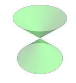
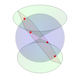
Figure 1: The varieties, over $\mathbb{R}$, corresponding to (4), (5), and (6) (respectively), and their intersection. Solution sets of nonlinear algebraic systems consisting of a finite number of points can be computed using Gröbner bases by recursively finding the roots of univariate polynomials.

m2r can be used to find all the solutions to this system exactly using Gröbner bases:

R> ring("x" ,"y", "z", coefring = "QQ")

M2 Ring: QQ[x,y,z], grevlex order

R> I <- ideal("x + y + z", "x^2 + y^2 + z^2 - 9", "x^2 + y^2 - z^2")
R> (grobner_basis <- gb(I))

x  +  y  +  z
2 z^2  -  9
y^2  +  y z

Notice that this system has one polynomial that only involves $z$, one that only involves $z$ and $y$, and one that involves $z$, $y$, and $x$. This is an example of the kind of nonlinear generalization of Gaussian elimination referred to in Section 2.

Once Macaulay2 computes a Gröbner basis, it is fairly straightforward to script a basic solver for nonlinear algebraic systems that recursively solves the univariate problems and plugs the solutions into the other equations to obtain other univariate problems. In general, when a problem can be reduced to determining the roots of a univariate polynomial, it is considered solved (Sturmfels, 2002). An implementation of a univariate polynomial root finder, the Jenkins-Traub method, is already available in base::polyroot(), which mpoly thinly wraps with solve_unipoly():

R> # create simple helpers
R> extract_unipoly <- function(mpolyList) Filter(is.unipoly, mpolyList)[[1]]
R> which_unipoly <- function(mpolyList) sapply(mpolyList, is.unipoly) %>% which
R> 
R> # create solver
R> solve_gb <- function(gb) {

+   # extract and solve univariate polynomial
+   poly <- extract˙unipoly(gb)
+   elim_var <- vars(poly)
+   solns <- solve˙unipoly(poly, real_only = TRUE)

+   # if univariate polynomial, return
+   if(length(gb) == 1) return(structure(t(t(solns)), .Dimnames = list(NULL, elim_var)))

+   # remove unipoly from gb; plug solns into remaining system to make new one
+   gb <- structure(gb[-which˙unipoly(gb)[1], drop = FALSE], class = "mpolyList")
+   new_systems <- lapply(solns, function(soln) plug(gb, elim_var, soln))

+   # solve reduced system
+   low_solns_list <- lapply(new_systems, solve_gb)
+   lower_var_names <- colnames(low_solns_list[[1]])

+   # aggregate solutions and return
+   Map(cbind, solns, low_solns_list) %>% do.call("rbind", .) %>%
+     structure(.Dimnames = list(NULL, c(elim_var, lower_var_names)))

+ }

The solver can then be applied to the system grobner_basis returned by gb() to compute the solutions to (4)–(6), the points of intersection of their corresponding varieties. We note that the solver above looks at the variety over $\mathbb{R}$, which is a field extension of $\mathbb{Q}$, the coefficient ring of the polynomial ring used.

R> (solns <- solve˙gb(grobner_basis)) %>%
+   structure(.Dimnames = list(paste("Soln", 1:4, ":"), c("z","y","x")))

                z        y        x
Soln 1 :  2.12132  0.00000 -2.12132
Soln 2 :  2.12132 -2.12132  0.00000
Soln 3 : -2.12132  0.00000  2.12132
Soln 4 : -2.12132  2.12132  0.00000

In closed form, the four solutions for $(x,y,z)$ are $\pm\frac{3}{\sqrt{2}}(1,0,-1)$ and $\pm\frac{3}{\sqrt{2}}(0,1,-1)$. Note that $\frac{3}{\sqrt{2}}\approx 2.12132$. These solutions can be easily checked by evaluating the original list of polynomials (4), (5), and (6). Moreover, the solutions printed above are accurate to 14 digits:

R> f <- as.function(grobner_basis, varorder = c("z","y","x"), vector = TRUE)
R> apply(solns, 1, f) %>% apply(2, round, digits = 14) %>%
+   structure(.Dimnames = list(paste("Eqn", 5:7, ":"), paste("Soln", 1:4)))

        Soln 1 Soln 2 Soln 3 Soln 4
Eqn 5 :      0      0      0      0
Eqn 6 :      0      0      0      0
Eqn 7 :      0      0      0      0

We note that a simple numerical strategy that uses general-purpose optimization routines to solve the system by minimizing the sum of the squares of the system not only finds only one solution but is also only correct to 3 digits:

R> r <- function(v) {
+   x <- v[1]; y <- v[2]; z <- v[3]
+   (x + y + z)^2 + (x^2 + y^2 + z^2 - 9)^2 + (x^2 + y^2 - z^2)^2
+ }
R> optim(c(x = 0, y = 0, z = 0), r)$par

            x             y             z
-2.1212603679  0.0002124893  2.1212744693

This problem is typically dramatically worse in real-world scenarios with more polynomials of higher degrees.

Though simple, in principle this application can be generalized to any system of nonlinear algebraic equations. With appropriate saturation, it can be generalized even further to systems of rational equations, i.e. systems involving ratios of multivariate polynomials. Saturation is key here because the basic strategy of clearing denominators, i.e. multiplying equations through by the least common multiple of the denominators to convert them into polynomial equations, typically introduces solutions where the original system was previously undefined. For example, the system $(\frac{y}{x}=1,y=x^{2})$ can be cleared to $(y=x,y=x^{2})$, which suggests the solutions $(0,0)$ and $(1,1)$; but $(0,0)$ cannot be a solution since the original system’s first equation ($\frac{y}{x}=1$) is not satisfied at $(0,0)$. Saturation removes this kind of problem.

New solvers are always of value to the R ecosystem, especially paradigmatically new solvers such as this Gröbner basis solution. One can imagine applications in disparate areas of statistics: computing estimators via estimating equations (including method of moments, maximum likelihood, and others), solving polynomial and rational optimization problems using Lagrange multipliers, and more. That being said, the Gröbner bases method has very definite limitations: the best algorithms are known to have worst-case behavior that is doubly-exponential in the number of variables, and solving systems of polynomial equations is in general known to be an NP-hard problem.

4.2 Independence and nonlinear algebra

One of the focal application domains of algebraic tools in statistics is the analysis of multiway contingency tables (Drton et al., 2009; Aoki et al., 2012). This is for several reasons. First, discrete probability distributions, often represented with probability mass functions in statistics, can be represented as algebraic objects: non-negative vectors that sum to one. The “sum to one” condition is a polynomial constraint on the vector of probabilities. Second, the definition of independence is an algebraic condition, as we will see below. Third, commutative algebra, particularly combinatorial commutative algebra, has many connections to integer lattices and polyhedral geometry, which is discussed a little more at the very end of this example.

A simple example of the algebraic structure of independence is provided by a two-way contingency table with variables $X$ and $Y$ and joint distribution $P\left[X=x,Y=y\right]=:p_{xy}$. If $X$ and $Y$ are both binary so that the sample space of both is $\mathcal{S}_{X}=\mathcal{S}_{Y}=\left\{0,1\right\}$, the situation is a $2\times 2$ table, and the probabilities are typically denoted $p_{00}$, $p_{01}$, $p_{10}$, and $p_{11}$. Collectively, these can be written in order as the column vector $\textbf{p}\in\mathbb{R}^{4}$ that must satisfy the condition

$$\textbf{1}_{4}^{\prime}\textbf{p}\ \ =\ \ p_{00}+p_{01}+p_{10}+p_{11}\ \ =\ \ 1.$$ (7)

If $X$ and $Y$ are independent, the joint distribution factors as a product of the marginals

$$p_{xy}\ \ =\ \ P\left[X=x,Y=y\right]\ \ =\ \ \Big{(}\sum_{y^{\prime}}P\left[X=x,Y=y^{\prime}\right]\Big{)}\Big{(}\sum_{x^{\prime}}P\left[X=x^{\prime},Y=y\right]\Big{)}\ \ =:\ \ p_{x+}p_{+y}.$$ (8)

Explicitly, independence demands four polynomial constraints of the probabilities:

$$p_{00} = (p_{00}+p_{01})(p_{00}+p_{10})$$ (9)

$$p_{01} = (p_{00}+p_{01})(p_{01}+p_{11})$$ (10)

$$p_{10} = (p_{10}+p_{11})(p_{00}+p_{10})$$ (11)

$$p_{11} = (p_{10}+p_{11})(p_{01}+p_{11}).$$ (12)

These conditions, along with the sum condition, are routinely summarized by statisticians in various ways: the log odds-ratio is zero ($\log\frac{p_{00}/p_{01}}{p_{10}/p_{11}}=0$), the odds-ratio is one ($\frac{p_{00}/p_{01}}{p_{10}/p_{11}}=1$), or the cross-product difference is zero ($p_{00}p_{11}-p_{01}p_{10}=0$) (Agresti, 2002). This last condition can be used to derive the other two. The distillation of (9)–(12) to the more simple cross-product condition $p_{00}p_{11}-p_{01}p_{10}=0$ can be systematically obtained through the process of computing a Gröbner basis. This can be done with gb():

R> ring("p00", "p01", "p10", "p11", coefring = "QQ")

M2 Ring: QQ[p00,p01,p10,p11], grevlex order

R> indep_ideal <- ideal(
+   "p00 - (p00 + p01) (p00 + p10)",    # p00 = (p00 + p01) (p00 + p10)
+   "p01 - (p00 + p01) (p01 + p11)",    # p01 = (p00 + p01) (p01 + p11)
+   "p10 - (p10 + p11) (p00 + p10)",    # p10 = (p10 + p11) (p00 + p10)
+   "p11 - (p10 + p11) (p01 + p11)",    # p11 = (p10 + p11) (p01 + p11)
+   "p00 + p01 + p10 + p11 - 1"         # simplex condition
+ )
R> gb(indep_ideal)

p00  +  p01  +  p10  +  p11  -  1
p01 p10  +  p01 p11  +  p10 p11  +  p11^2  -  p11

Note that the last equation is the one of interest:

$$p_{01}p_{10}+p_{01}p_{11}+p_{10}p_{11}+p_{11}^{2}-p_{11}\ \ =\ \ p_{01}p_{10}+(p_{01}+p_{10}+p_{11}-1)p_{11}\ \ =\ \ p_{01}p_{10}-p_{00}p_{11}.$$ (13)

In addition to the specification of the model, Macaulay2 can use algebraic techniques to determine the dimension of the variety corresponding to the ideal:

R> dimension(indep_ideal)

[1] 2

It is well-known that the asymptotic distribution of many test statistics (e.g. Pearson’s $\chi^{2}$, the likelihood-ratio $G^{2}$, etc.) depends on the difference between the dimension of the saturated model, which is the dimension of the simplex, and the dimension of the model. In this case, that distribution is $\chi^{2}_{\nu}$, where $\nu$ is the difference. The dimension of the saturated model is $4-1=3$, where one degree of freedom is lost to the simplex condition. (This can also be checked with dimension(ideal("p00 + p01 + p10 + p11 - 1")).) Thus, the asymptotic distribution of those test statistics is $\chi^{2}_{3-2}=\chi^{2}_{1}$, which is consistent with the presentation in introductory courses.

While this example is restricted to independence in the $2\times 2$ case, it generalizes fully to not only $r\times c$ tables but also to the multiway case and conditional independence models, a large class that subsumes graphical models and hierarchical loglinear models. Partial independence models, where conditional independence statements do not hold for every level, are also included in this description, as are conditional independence models with structural zeros. In short, working directly with the enumerated polynomial conditions implied by independence and conditional independence statements expands the horizons of discrete multivariate analysis. This also has ramifications for computing estimators (see Kahle (2011) for details).

One of the most well-developed areas of the young field of algebraic statistics is that of Markov bases. Imprecisely, a Markov basis is a collection of contingency tables called moves that, when added to a given contingency table, result in another contingency table with the same marginals. Marginals can be meant in the ordinary sense of row and column sums for two-way tables, or in a more generalized sense for more complex models on multiway tables. Given a Markov basis, in principle one can easily construct a Markov chain Monte Carlo (MCMC) algorithm to sample from any distribution on the set of tables with the same marginals as the given table, a set called the fiber of the table. This in turn can be used to generalize Fisher’s exact test, which is used to test for independence in $2\times 2$ tables, to any discrete exponential family model on any multiway table, an enormous generalization. A foundational result in algebraic statistics called the Fundamental Theorem of Markov Bases implies that Markov bases can be computed as Gröbner bases of a special ideal (Diaconis and Sturmfels, 1998). While latter’s connection to 4ti2 allows for these kinds of computations, m2r’s gb() gives the user much more flexibility in these kinds of computations, albeit at significantly reduced performance (Kahle et al., 2016; 4ti2 Team, 2015).

5 Internals and design philosophy

The m2r package was designed with three basic principles in mind: (1) make Macaulay2 as R-user friendly as possible, (2) be as flexible with Macaulay2 syntax and data structures possible, and (3) minimize computational overhead. We advance these goals with a functional approach by including new data structures, a robust Macaulay2 parser, lazy parsing, and reference functions. In this section we describe these in just enough detail to explain how they work at a basic level. For more information, we direct the reader to the GitHub page at https://github.com/coneill-math/m2r.

5.1 m2r data structures

One of the challenges of working with a computer algebra system in R is that R has no infrastructure to handle algebraic objects. mpoly alleviates this, but only for polynomials. There is still a world of other algebraic objects, such as those described in Section 2, that are represented in computer algebra systems but do not have any natural analogue in the R ecosystem.

In Section 5.2 we describe how m2r converts Macaulay2 data into R objects; however, before that discussion it helps to have an understanding of what kinds of objects m2r parses Macaulay2 code into. Most objects parsed from Macaulay2 back into R are S3 objects whose last class type is "m2" and whose other class types describe the object in decreasing order of specificity. For example:

R> str(R)

Classes ’m2_polynomialring’, ’m2’  atomic [1:1] NA
  ..- attr(*, "m2_name")= chr "m2rintring00000001"
  ..- attr(*, "m2_meta")=List of 3
  .. ..$ vars    :List of 4
  .. .. ..$ : chr "t"
  .. .. ..$ : chr "x"
  .. .. ..$ : chr "y"
  .. .. ..$ : chr "z"
  .. ..$ coefring: chr "QQ"
  .. ..$ order   : chr "grevlex"

Created in Section 3.2, R represents the polynomial ring $\mathbb{Q}[t,x,y,z]$. As algebraic objects, rings have no natural analogue in R, so m2r needs to provide a data structure to represent them. R is an S3 object of class c("m2_polynomialring", "m2"). The value of the object is NA, a logical(1) vector; this prevents R users from naively operating on the ring itself. m2r typically represents algebraic objects by parsing them into R as NA with two attributes, a name (m2_name) and a list of metadata (m2_meta). Both have accessor functions:

R> m2˙name(R)

[1] "m2rintring00000001"

R> m2˙meta(R) %>% str

List of 3
 $ vars    :List of 4
  ..$ : chr "t"
  ..$ : chr "x"
  ..$ : chr "y"
  ..$ : chr "z"
 $ coefring: chr "QQ"
 $ order   : chr "grevlex"

The m2_name attribute is the Macaulay2 variable binding for the object; it’s the name of the object on the Macaulay2 side. The m2_meta attribute contains other information about the object for easy R referencing.

Almost every object returned by m2r functions behaves this way with one major exception: when the object has a natural analogue in R. For example, both R and Macaulay2 have integers and integer matrices, so it makes sense that when a Macaulay2 integer matrix is parsed back into R, R users can manipulate it just like an ordinary R integer matrix. And that is in fact what m2r parses the object into, but m2r makes sure that the object retains the knowledge that it is a Macaulay2 object. For example, the integer matrix P created in the Smith normal form example in Section 3.4 is such an object:

R> P

     [,1] [,2] [,3]
[1,]    1    0    1
[2,]    0    1    0
[3,]    0    0    1
M2 Matrix over ZZ[]

R> str(P)

 int [1:3, 1:3] 1 0 0 0 1 0 1 0 1
 - attr(*, "class")= chr [1:3] "m2_matrix" "m2" "matrix"
 - attr(*, "m2_name")= chr ""
 - attr(*, "m2_meta")=List of 1
  ..$ ring:Classes ’m2_polynomialring’, ’m2’  atomic [1:1] NA
  .. .. ..- attr(*, "m2_name")= chr "ZZ"
  .. .. ..- attr(*, "m2_meta")=List of 3
  .. .. .. ..$ vars    : NULL
  .. .. .. ..$ coefring: chr "ZZ"
  .. .. .. ..$ order   : chr "grevlex"

This is what allowed us to compute its determinant directly in Section 3.4 with det(P).

5.2 The Macaulay2 parser

Each call to Macaulay2 via the m2() function produces a string representing a Macaulay2 object. This string, returned from the toExternalString function in Macaulay2, consists of valid Macaulay2 syntax used to recreate the object it represents, analogous to R’s dput(). Though this string is useful for subsequent Macaulay2 calls because Macaulay2 understands it, it typically needs to be parsed in order to be useful to the R user. This task is tedious to do by hand and requires an understanding of Macaulay2 syntax.

m2_parse() is m2r’s general-purpose parsing function. It takes as input a string of Macaulay2 output (such as one returned from toExternalString) and returns a corresponding object in R. For example, given a string produced from passing a Macaulay2 matrix to Macaulay2’s toExternalString, m2_parse() returns a native R matrix as part of the larger c("m2_matrix", "m2") data structure.

The parser is one of the primary features of m2r. It was designed to be as extensible as possible, so that new features could be added easily and quickly. For example, in order to add support for the Macaulay2 type ideal, which is returned from Macaulay2 as a string of the form

ideal map((R)^1,(R)^{{-3},{-3},{-3}},{{a*b*c-d*e*f, a*c*e-b*d*f}}),

the user simply implements m2_parse_function.m2_ideal(), a single method for the m2_parse_function() S3 generic that the parser calls when it encounters an ideal object. This particular function is built in:

R> m2_parse_function.m2_ideal <- function(x) {
+   m2˙structure(
+     m2_name = "",
+     m2_class = "m2_ideal",
+     m2_meta = list(rmap = x[[1]])
+   )
+ }

m2_structure() accepts five arguments: x, the value of the returned object that is defaulted to NA; m2_name, the name of the object; m2_class, the higher precedent class; m2_meta, the list of metadata; and base_class, for higher order classes. In general specific m2_parse_function() methods accept a list of arguments x to the Macaulay2 function ideal(); in this case this consists of a single one-row matrix object. When the method is dispatched as part of m2_parse(), the parser has already parsed the map(...) substring to construct an R-matrix whose entries are mpoly objects and passed this via x[[1]]. The returned m2_structure thus encapsulates the m2_ideal object and has a list of mpoly objects as its metadata for each polynomial generator of the ideal.

The recursive nature of the parser effectively black-boxes most of its inner workings, so that adding new features does not require a deep understanding of the parser’s internal structure (e.g. the tokenizer). Indeed, much of the currently supported m2r functionality (including matrix and ideal objects) uses functions like these, built directly into the parser. This high level of extensibility ensures that adding new features is quick and uniform, while requiring as little additional code as possible. Its simplicity also encourages contributions from other developers through the m2r GitHub page.

5.3 Lazy parsing and reference functions

As noted in Section 1, one of the primary benefits of Macaulay2 is its efficiency with large algebraic computations. For instance, some Gröbner basis computations can take many hours and produce output consisting of several thousand polynomials or polynomials with several thousand terms. The Macaulay2 user can specify properties to return or have the output immediately passed into another function.

In order to avoid the computational overhead of copying and parsing large data structures into R, only to then convert them back to Macaulay2 for subsequent function calls, nearly every m2r function has two versions: a reference version and a value version. Until now, every m2r function we have seen has been the value version. As a general naming convention, the reference version of a function is the value version’s name followed by a dot. For example, gb.() is the reference function corresponding to the value function gb().

So what is the difference? Unlike value functions, reference functions return a pointer to a Macaulay2 data structure, an S3 object of class c("m2_pointer","m2"). In general, pointers are not very helpful on the R side; they are difficult to interpret and have somewhat complex printing methods. For example, the reference version of gb() has the following output:

R> gb.(I)

M2 Pointer Object
  ExternalString : map((m2rintring00000004)^1,(m2rintring00000004)^{{-1...
         M2 Name : m2rintgb00000006
        M2 Class : Matrix (Type)

Obviously, the output does not appear particularly useful; it gives no clues as to what the Gröbner basis actually is. Pointers are used as R-side handles for Macaulay2-side objects.

Most of the time, the pointer returned from a reference function is passed into m2_parse() to produce the corresponding R types. (The exception to this is m2() itself, which simply returns the external string part of the pointer returned by m2.().) In fact, this is precisely what value versions of functions do; they thinly wrap reference versions with an m2_parse() call, occasionally with additional parsing. But users can also pass pointers directly into nearly any m2r function and obtain the same output without requiring a computationally expensive call to m2_parse().

With this design, a novice user can avoid any confusion associated with pointers by simply omitting the trailing “.” from any functions they use, and their code will work as expected. However, advanced users have the option to save additional overhead by using the reference functions (those ending in “.”) when they intend to immediately pass the output back into another m2r function.

6 The m2r cloud

Ultimately, every m2r function that uses Macaulay2 invokes m2.(). Every time m2.() is called, it checks for a connection to a live Macaulay2 instance. If one is not found, start_m2() is run to initialize the Macaulay2 session. In this section we describe how m2r makes this connection between R and Macaulay2. We begin with the basic mechanism of connection, sockets, and then turn to how these connections support a cloud computing framework that migrates computations off-site, enabling Macaulay2 through m2r for Windows users, among other things.

6.1 The socket connection between R and a local Macaulay2 instance

m2r uses sockets as the primary form of communication between concurrent R and Macaulay2 sessions. A socket is a low-level transfer mechanism used for interprocess communication. Sockets are commonly used to send and receive data over the internet, but they can also be used to transfer data between processes running on the same machine. Sockets on a given machine are identified by their port number. To initiate a connection, one endpoint (the server) must open a port for incoming connections, to which the other endpoint (the client) can then connect. Communication through a socket is anonymous; a process need not know the location of the other endpoint when it connects to the socket, sends and receives data through the socket, or closes its connection.

The socket setup has two key advantages. First and foremost, it enables a single tethered Macaulay2 session to persist for the duration of the active R session, so any variables or functions the user defines in Macaulay2 remain available for future use. Second, the resulting implementation can be easily extended to run the R and Macaulay2 sessions on different machines, we explore this in the next section.

When start_m2() is called it attempts to initiate a socket connection between R and Macaulay2 using the sequence of events documented in Figure 2. Once R successfully binds to the socket opened by Macaulay2, the basic infrastructure is in place for R to send Macaulay2 code as character strings to be evaluated; each such code snippet $L$ is simply relayed to Macaulay2 through the socket. After Macaulay2 evaluates $L$, it constructs and returns a string $S$ containing (i) any error codes, (ii) the number of lines of output, and (iii) the output; see Figure 3 for an illustration.

(a) R begins by launching an M2 instance, then waits for an available connection on the specified port.

(b) Once launched, M2 opens a socket on the specified port and waits for a connection to be established.

(c) R connects to the socket, and M2 pauses while it waits to receive data through the socket.

(d) Upon successfully connecting to the socket, R returns control to the user until m2() is called.

Figure 2: The socket connection process.

(a) R sends a Macaulay2 source string $L$ through the socket, and then waits for a response from M2.

(b) M2 evaluates $L$, sends its response $S$ back through the socket, and then resumes listening.

Figure 3: Messages are passed back and forth through the socket.

After Macaulay2 issues $S$ it is relayed through the socket to R, which handles any errors and returns the output to the user. When the R session terminates (or m2_stop() is called by the user), the socket connection is closed by R sending an empty string through the socket signaling end of file (EOF). Upon receiving an empty string and an EOF signal, Macaulay2 closes the socket connection and exits quietly. These steps cleanly kill the Macaulay2 process spawned by R so that no Macaulay2 processes remain orphaned after the R session is terminated.

It is also important to note that the script run by the spawned Macaulay2 process does not directly contain any user-supplied code. Instead, a Macaulay2 script that establishes the socket connection with R and conforms to all steps outlined above is run.

6.2 Macaulay2 in the cloud

Cloud computing as a service has come into prominence in recent years through the widespread availability of high speed internet connections and the decreasing cost of hardware and its maintenance at scale, among other things. In a cloud computing model, the users of a software system do not need to download the software which they are using, instead they can simply interact with the software of interest via a web or terminal interface. Users call on the remote machine to perform a calculations, and when the remote computations finish the results are returned to the user.

The core benefit of a cloud computing model for m2r is that users no longer have to install Macaulay2 on their local machines. Installing specialized software can be difficult and time consuming, especially for less computer-savvy users, and this can be an insurmountable barrier to entry to algebraic statistics and algebraic methods in general. This issue is compounded for new users who are not sure if a certain software is the correct solution for their problem and so are unwilling to invest the time. Installing Macaulay2 on a Windows machine is an especially arduous task, creating an enormous barrier to entry for potential Windows users of the package. These are common challenges for specialized mathematical software, and like others before us we concluded that a cloud version of our software was a worthwhile venture (Bliss et al., 2015; Kastner et al., 2015).

Amazon Web Services (AWS, available at https://aws.amazon.com/) is a subsidiary of Amazon, Inc. that sells cloud computing solutions. AWS’s flagship product is the Amazon Elastic Compute Cloud (EC2), which provides virtual servers of varying performance specs that can be launched remotely on demand. To help users get up and running with m2r and algebraic statistical computing, we have set up a low-performance EC2 instance dedicated to m2r. We chose to use the introductory tier of this product because it suffices for introducing R users to Macaulay2 and Amazon offers it at no cost. It also provides a proof-of-concept model that can be replicated for a user’s own personal cloud. Instructions for setting up such an instance can be found on m2r’s GitHub page (https://github.com/coneill-math/m2r/, under inst/).

A few noteworthy implementation details for remotely running m2r are in order. Each remote instance of Macaulay2 is run within a virtual machine managed by Docker (https://www.docker.com), an open source software package that allows for sandboxing of applications inside distinct lightweight virtual software containers. Docker containers provide an additional layer of virtualization that isolates key resources of the host machine. This safeguards the host machine in the sense that nothing executed in a container can affect the host machine. Additionally, containers are optimized to be spun up quickly through efficient usage of host machine resources, significantly decreasing the time necessary to start a new session and allowing m2r to connect to on-demand instances of Macaulay2 in seconds.

While there are many similarities in how m2r connects R to local and remote Macaulay2 instances, there are some important differences as well. Instead of the typical m2r flow where an instance of Macaulay2 is launched on the user’s local machine, the server version allows a user to create on-demand Macaulay2 instances on an active EC2 instance. In addition to running and managing all active Docker containers, the EC2 instance has a Python server script that is used to spawn new Docker instances and dispatch ports to new clients. The connection process for a new R client is diagrammed step-by-step in Figure 4.

(a) The client R session connects to the Python server running on the EC2 instance using a static port. The Python server immediately locates an open and unoccupied port $p$ on the EC2 instance.
 

(b) The Python server launches a new Docker container provisioned with Macaulay2 and other helpful software. Within this sandboxed container, Macaulay2 is launched and given $p$ as the port number on which to expect an incoming connection.

(c) The Python server sends $p$ to the R client, terminates its connection, and begins listening for connections from the next new R client.

(d) The R client, upon receiving $p$ from the Python server, connects via port $p$ to the Macaulay2 instance running in the new Docker container using the same paradigm used for local Macaulay2 instances.

Figure 4: How R connects to a Macaulay2 session on a remote EC2 host.

The first time m2.() is run, m2r will automatically connect to the cloud if no local Macaulay2 installation is detected. Note that this will always be the case on a Windows machine, since running a local instance of Macaulay2 is not supported. To bypass a local installation and connect to the cloud, use the cloud parameter to start_m2().

R> stop˙m2()
R> start˙m2(cloud = TRUE)

Connecting to M2 in the cloud...

done.

R> m2("1+1")

[1] "2"

If the user has the Macaulay2 server script running on their own EC2 instance (or any other cloud service for that matter), the URL can be specified with the hostname parameter to start_m2(). From there, everything will work just as if the user were running a local Macaulay2 instance.

7 Future directions

In this article we have introduced the new m2r R package, demonstrated several ways it can be used, and explained how it works. There are several directions of future development that we are excited about, including performance enhancements for the parser, support for features such as arbitrary precision numbers and arithmetic with gmp (Granlund and the GMP Development Team, 2012; Lucas et al., 2017), modifications to mpoly for broader support for multivariate polynomials in R (e.g. matrices of multivariate polynomials), and more. Macaulay2 boasts a number of packages for algebraic statistics that are ripe for implementation and of interest to R users and the statistics community more broadly. We invite collaborators to contact us directly and share their ideas on the GitHub page.

References

- 4ti2 Team (2015) 4ti2 Team, 2015. 4ti2—a software package for algebraic, geometric and combinatorial problems on linear spaces. Available at www.4ti2.de.
- Agresti (2002) Agresti, A., 2002. Categorical Data Analysis, 2nd Edition. John Wiley & Sons.
- Améndola et al. (2016) Améndola, C., Faugère, J.-C., Sturmfels, B., 2016. Moment varieties of gaussian mixtures. Journal of Algebraic Statistics 7 (1), 14–28.
- Aoki et al. (2012) Aoki, S., Hara, H., Takemura, A., 2012. Markov Bases in Algebraic Statistics. Vol. 199. Springer.
-
Bache and Wickham (2014)
Bache, S. M., Wickham, H., 2014. magrittr: A Forward-Pipe Operator for R. R
package version 1.5.
URL https://CRAN.R-project.org/package=magrittr - Bliss et al. (2015) Bliss, N., Sommars, J., Verschelde, J., Yu, X., 2015. Solving polynomial systems in the cloud with polynomial homotopy continuation. In: Gerdt, V., Koepf, W., Mayr, E., Vorozhtsov, E. (Eds.), Computer Algebra in Scientific Computing, 17th International Workshop, CASC 2015. Vol. 9301 of Lecture Notes in Computer Science. pp. 87–100.
-
Bondesson (1983)
Bondesson, L., 1983. Equivariant Estimators. John Wiley & Sons, Inc.
URL http://dx.doi.org/10.1002/0471667196.ess0562.pub2 - Bruns et al. (2015) Bruns, W., Ichim, B., Römer, T., Sieg, R., Söger, C., 2015. Normaliz. algorithms for rational cones and affine monoids. Available at https://www.normaliz.uni-osnabrueck.de.
- Bruns et al. (2016) Bruns, W., Ichim, B., Söger, C., 2016. The power of pyramid decomposition in normaliz. Journal of Symbolic Computation 74, 513–536.
- Bruns and Kämpf (2010) Bruns, W., Kämpf, G., 2010. A macaulay2 interface for normaliz. Journal of Software for Algebra and Geometry 2, 15–19.
- Buchberger (1970) Buchberger, B., 1970. An algorithmic criterion for the solvability of algebraic systems of equations (german). Aequationes Mathematicae 4, 374–383.
- Cox et al. (1997) Cox, D., Little, J., O’Shea, D., 1997. Ideals, Varieties, and Algorithms, 2nd Edition. Springer, New York.
- Diaconis and Sturmfels (1998) Diaconis, P., Sturmfels, B., 1998. Algebraic algorithms for sampling from conditional distributions. The Annals of Statistics 26 (1), 363–397.
- Drton et al. (2009) Drton, M., Sturmfels, B., Sullivant, S., 2009. Lectures on Algebraic Statistics. Birkhauser Basel.
- Fisher (1934) Fisher, R. A., 1934. Statistical methods for research workers, 5th Edition. Oliver & Boyd, Edinburgh.
- Gallian (2016) Gallian, J., 2016. Contemporary abstract algebra, 9th Edition. Cengage Learning.
-
Granlund and the GMP Development Team (2012)
Granlund, T., the GMP Development Team, 2012. GNU MP: The GNU
Multiple Precision Arithmetic Library. 5th Edition.
URL http://gmplib.org/ - Grayson and Stillman (2006) Grayson, D. R., Stillman, M. E., 2006. Macaulay2, a software system for research in algebraic geometry. Available at http://www.math.uiuc.edu/Macaulay2/.
- Greuel et al. (2006) Greuel, G. M., Pfister, G., Schoenemann, H., 2006. Singular: A computer algebra system for polynomial computations. http://www.singular.uni-kl.de.
- Gross et al. (2013) Gross, E., Petrović, S., Verschelde, J., 2013. Interfacing with phcpack. Journal of Software for Algebra and Geometry 5, 20–25.
-
Grothendieck and Bellosta (2012)
Grothendieck, G., Bellosta, C. C. J. G., 2012. rSymPy: R interface to SymPy
computer algebra system. R package version 0.2-1.1.
URL https://CRAN.R-project.org/package=rSymPy - Kahle (2011) Kahle, D., 2011. Minimum distance estimation in categorical conditional independence models. Ph.D. thesis, Rice University.
-
Kahle (2013)
Kahle, D., 2013. mpoly: Multivariate polynomials in R. The R Journal 5 (1),
162–170.
URL http://journal.r-project.org/archive/2013-1/kahle.pdf - Kahle et al. (2016) Kahle, D., Garcia, L., Yoshida, R., 2016. latter: LattE and 4ti2 in R. R package version 0.1.0.
- Kahle et al. (2014) Kahle, D., Garcia-Puente, L., Yoshida, R., 2014. algstat: Algebraic statistics in R. R package version 0.1.0.
- Kastner et al. (2015) Kastner, L., Hinkelmann, F., Stillman, M., 2015. A web application for macaulay2.
- Lehmann and Romano (2005) Lehmann, E. L., Romano, J. P., 2005. Testing statistical hypotheses, 3rd Edition. Springer Texts in Statistics. Springer, New York.
-
Lucas et al. (2017)
Lucas, A., Scholz, I., Boehme, R., Jasson, S., Maechler, M., 2017. gmp:
Multiple Precision Arithmetic. R package version 0.5-13.1.
URL https://CRAN.R-project.org/package=gmp -
Lumley (2003)
Lumley, T., 2003. Standard Nonstandard Evaluation Rules.
URL https://developer.r-project.org/nonstandard-eval.pdf -
Meurer et al. (2017)
Meurer, A., Smith, C. P., Paprocki, M., Čertík, O., Kirpichev, S. B.,
Rocklin, M., Kumar, A., Ivanov, S., Moore, J. K., Singh, S., Rathnayake, T.,
Vig, S., Granger, B. E., Muller, R. P., Bonazzi, F., Gupta, H., Vats, S.,
Johansson, F., Pedregosa, F., Curry, M. J., Terrel, A. R., Roučka, v.,
Saboo, A., Fernando, I., Kulal, S., Cimrman, R., Scopatz, A., Jan. 2017.
Sympy: symbolic computing in python. PeerJ Computer Science 3, e103.
URL https://doi.org/10.7717/peerj-cs.103 - Pearson (1894) Pearson, K., 1894. Contributions to the mathematical theory of evolution. Philosophical Transactions of the Royal Society of London. A 185, 71–110.
- Pitman (1939) Pitman, E. J. G., 1939. Tests of hypotheses concerning location and scale parameters. Biometrika 31 (1/2), 200–215.
-
R Core Team (2014)
R Core Team, 2014. R: A Language and Environment for Statistical Computing. R
Foundation for Statistical Computing, Vienna, Austria.
URL http://www.R-project.org/ - Sturmfels (1996) Sturmfels, B., 1996. Gröbner Bases and Convex Polytopes. Vol. 8 of University Lecture Series. American Mathematical Society, Providence, RI.
- Sturmfels (2002) Sturmfels, B., 2002. Solving Systems of Polynomial Equations. American Mathematical Society, Providence, Rhode Island.
- Verschelde (1999) Verschelde, J., 1999. Algorithm 795: Phcpack: A general-purpose solver for polynomial systems by homotopy continuation. ACM Trans. Math. Softw. 25, 251–276.
- Wickham (2014) Wickham, H., 2014. Advanced R. CRC Press.
-
Wickham (2017)
Wickham, H., 2017. stringr: Simple, Consistent Wrappers for Common String
Operations. R package version 1.2.0.
URL https://CRAN.R-project.org/package=stringr -
Wickham and Francois (2016)
Wickham, H., Francois, R., 2016. dplyr: A Grammar of Data Manipulation. R
package version 0.5.0.
URL https://CRAN.R-project.org/package=dplyr