Reconstructing $f(R)$ Gravity from a Chaplygin Scalar Field in de Sitter Spacetimes

Abstract

We present a reconstruction technique for models of $f(R)$ gravity from the Chaplygin scalar field in flat de Sitter spacetimes. Exploiting the equivalence between $f(R)$ gravity and scalar-tensor theories, and treating the Chaplygin gas as a scalar field model in a universe without conventional matter forms, the Lagrangian densities for the $f(R)$ action are derived. Exact $f(R)$ models and corresponding scalar field potentials are obtained for asymptotically de Sitter spacetimes in early and late cosmological expansion histories. It is shown that the reconstructed $f(R)$ models all have General Relativity as a limiting solution.

PACS: 04.50.Kd, 04.25.Nx, 98.80.-k, 95.36.+x, 98.80.Cq

1 Introduction

The standard model of cosmology with $\Lambda$CDM fits a number of observational data very well [1]. The rapid development of observational cosmology recently has shown that the Universe has undergone two phases of cosmic accelerated expansion. The first one is the so-called inflation [2, 3, 4] which is understood to have occurred prior to the radiation-dominated era [5]. This phase is required not only to solve the flatness and horizon problems plagued in standard Big Bang cosmology, but also to explain a nearly flat spectrum of temperature anisotropies observed in the CMB [6]. The second accelerating expansion phase has started after the matter-domination era, which implies that the pressure $p$ and the energy density $\mu$ of the universe should have violated the strong physical energy condition $\mu+3p>0$ [7]. Therefore, this late cosmic acceleration cannot be explained by the presence of standard matter whose equation of state $w=p/\mu$ satisfies the condition $w\geq 0$. In fact, we need a component of negative pressure with at least $w<-1/3$ to realise the acceleration of the universe. This unknown smooth component responsible for this acceleration in the expansion rate is referred to as “dark energy” [8]. The need for the existence of dark energy has been confirmed by a number of observations such as SN Ia [7, 9], the LSS [10, 11], the BAO [12], and the CMB [13].

However, there are numerous recent attempts to explain away dark energy. Two of the most common such attempts come either in the form of modifications to the theory of gravity or the introduction of new matter or scalar field contributions to the action of General Relativity (GR). In the latter case, one suggestion is that the change in the behavior of the missing energy density might be regulated by the change in the equation of state of the background fluid instead of the form of the potential [14, 15]. The Chaplygin Gas (CG) model in cosmology is one of the most profound candidates for this suggestion. For quite sometime now, the CG model has been considered as another alternative to the cosmological FLRW universe models with a perfect fluid equation of state and negative pressure [16, 17]. The model provides interesting features of the cosmic expansion history consistent with a smooth transition between an inflationary phase and a matter-dominated decelerating era. In addition, the late-time accelerated de Sitter phase of cosmic expansion can be achieved [18, 19, 20, 21].

Among the earliest and simplest modifications to the GR gravitational action are $f(R)$ gravity models. These models are usually considered to be geometrical alternatives to the dark energy debate [22, 23, 24, 25, 26, 27, 28, 29, 30], but their scopes of applicability has only been increasing: from early-universe cosmic inflation [2, 31, 32], to the evolutionary dynamics of large-scale structure [33, 34, 35, 36, 37, 38, 39, 40, 41] and astrophysics [42, 43, 44, 45].

An interesting aspect of $f(R)$ gravitational models is their proven equivalence to a class of the Brans-Dicke (BD) version of scalar-tensor (ST) theories [46, 47, 48, 49]. The main objective of this paper is to make use of this equivalence and reconstruct models of $f(R)$ gravity that describe exactly the same background cosmological evolution as Chaplygin gas models that mimic a BD scalar field with a vanishing coupling constant.

The remaining part of the manuscript is organised as follows: in Section 2, we will give a brief description of the three underlying alternative cosmological theories used for our analysis, namely, $f(R)$ models of gravity, the Chaplygin gas as a cosmological solution and the BD classes of ST theories. After solving the background fluid equations for the Chaplygin gas playing the role of a classical scalar field, which in turn is linked to the $f(R)$ gravitational models through the correspondence described above, we reconstruct the $f(R)$ functionals in Section 3 for the original Chaplygin gas model and section 4 is devoted to $f(R)$ functionals for the generalized Chaplygin gas model. The general solutions are highly intractable, but we provide exact solutions in asymptotic regimes: early-time and far-future cosmologies. We have applied these solutions to de Sitter spacetimes, where exact potential forms as functions of both the scalar field and the scale factor are analysed, followed by discussions and conclusions in Section 5.

In this paper, we will frequently use the natural units convention ($\hbar=c=k_{B}=8\pi G=1$) and Latin indices $a\;,b\;,c\;,\dots$ run from 0 to 3. The symbols $\nabla$, $\tilde{\nabla}$ and the overdot ^. represent, respectively, the usual covariant derivative, the spatial covariant derivative, and differentiation with respect to cosmic time. We use the $(-+++)$ spacetime signature and the Riemann tensor is defined by

$$R^{a}_{bcd}=\Gamma^{a}_{bd,c}-\Gamma^{a}_{bc,d}+\Gamma^{e}_{bd}\Gamma^{a}_{ce}-\Gamma^{f}_{bc}\Gamma^{a}_{df}\;,$$ (1)

where the $\Gamma^{a}_{bd}$ are the Christoffel symbols (i.e., symmetric in the lower indices) defined by

$$\Gamma^{a}_{bd}=\frac{1}{2}g^{ae}\left(g_{be,d}+g_{ed,b}-g_{bd,e}\right)\;.$$ (2)

The Ricci tensor is obtained by contracting the first and the third indices of the Riemann tensor:

$$R_{ab}=g^{cd}R_{cadb}\;.$$ (3)

Unless otherwise stated, primes ${}^{{}^{\prime}}\;,^{{}^{\prime\prime}}$ etc are shorthands for derivatives with respect to the Ricci scalar

$$R=R^{a}{}_{a}\;$$ (4)

and $f$ is used as a shorthand for $f(R)$.

2 Three alternative cosmological theories

In this section, we are going to briefly review the three alternative theories of gravity, namely $f(R)$ gravity, ST theory and the Chaplygin-gas model. These gravity theories have been suggested and studied with the intention of showing that they can mimic both the dark matter and dark energy mysteries.

2.1 Equivalence between $f(R)$ and scalar-tensor theories

The scalar-tensor theory of gravity is a theory which tries to explain the interactions of gravity with matter. It is through this that the $f(R)$ gravity theory has been shown to be a sub-class of the ST theory [48]. A clear illustration of how $f(R)$ theories are classified as a subclass of ST theory is in the BD theory for the case of the coupling constant $\omega=0$ [50]. The action in BD theory is given such that $\omega$ is independent of the scalar field [29, 28]. Thus, we have

$$I_{BD}=\frac{1}{2\kappa}\int d^{4}x\sqrt{-g}\left[\phi R-\frac{\omega}{\phi}\nabla_{\mu}\phi\nabla^{\mu}\phi+\mathcal{L}_{m}(\Psi,g_{\mu\nu})\right]\;,$$ (5)

where $\kappa=8\pi G$, $R$ is the Ricci scalar and $\mathcal{L}_{m}$ is the matter Lagrangian. We consider the action that represents $f(R)$ gravity given as

$$I=\frac{1}{2\kappa}\int d^{4}x\sqrt{-g}\left[f(R)+\mathcal{L}_{m}\right]\;.$$ (6)

The action in ST theory has the form [51, 52]:

$$I_{f(\phi)}=\frac{1}{2\kappa}\int d^{4}\sqrt{-g}\left[f(\phi(R))+\mathcal{L}_{m}\right]\;,$$ (7)

where $f(\phi(R))$ is a function of $\phi(R)$ and we consider the scalar field $\phi$ to be [52, 49]

$$\phi=f^{\prime}-1\;.$$ (8)

Here, the scalar field $\phi$ should be invertible [53, 50, 48]. Thus, if we compare the ST theory action to Eq. (5) of the BD theory for the case of a vanishing coupling constant $\omega=0$, we can say that $f(R)$ theory is a special case of the ST theory. One can use the Palatini approach to show that $f(R)$ is a sub-class of ST theory but in that context, the coupling constant is considered to be $\omega=-\frac{3}{2}$ (see more detail in Refs. [53, 54]).

In this paper, we consider the treatment of the Chaplygin gas as a scalar fluid. With this in mind, we can make a basic analysis of the Chaplygin gas through the ST theory of gravity. From the motivation that an equivalence between scalar-tensor theory (BD-theory) and $f(R)$ theory of gravity exists, we obtain the energy density of the Chaplygin gas in terms of the scalar field, and from the Chaplygin gas property, we obtain the Chaplygin gas pressure. The reason behind this treatment is that, in the literature, a lot of work has been done that suggests that the Chaplygin gas can be treated as dark matter [16, 17, 18, 19, 20, 21].

2.2 Chaplygin gas model

In the original treatment, the negative pressure associated with the Chaplygin-gas model is related to the (positive) energy density through the EoS [30, 20, 16]

$$p=-\frac{A}{\mu}\;,$$ (9)

where $A$ is a positive constant. Using this equation of state in the conservation equation of $\mu$ given by

$$\dot{\mu}+3\frac{\dot{a}}{a}\left(\mu+p\right)=0\;,$$ (10)

we find that the energy density of the Chaplygin gas evolves w.r.t the scale factor $a(t)$ as

$$\mu(a)=\sqrt{A+\dfrac{B}{a^{6}}}\;,$$ (11)

where $B$ is a constant of integration. One can see that for large $a(t)$, the energy density becomes independent of the scale factor for positive $B$. This can be thought of as an empty universe with a cosmological constant (see more detailed analysis in Ref. [20]). In Ref. [20], it has been pointed out that for the early universe, the approximated expression of energy density can represent a universe that contains pressureless dust matter. From the Friedmann equation

$$\Big{(}\dfrac{\dot{a}}{a}\Big{)}^{2}=\dfrac{\mu}{3}-\dfrac{k}{a^{2}}\;,$$ (12)

where $k$ stands for curvature and can be either $-1,0$ or $1$, depending on the spacetime geometry. If we restrict ourselves to the case where the universe is flat, i.e., $k=0$, then

$$\dot{a}=a\sqrt{\dfrac{\mu}{3}}\;.$$ (13)

The energy density of the scalar field and pressure are given as [55, 16]

$$\mu_{\phi}=\dfrac{1}{2}\dot{\phi^{2}}+V(\phi)\;,$$ (14)

$$p_{\phi}=\dfrac{1}{2}\dot{\phi^{2}}-V(\phi)\;.$$ (15)

Adding Eqs. (14) and (15) and using Eq. (11), we get

$$\dot{\phi^{2}}=\frac{B}{a^{3}\sqrt{Aa^{6}+B}}\;.$$ (16)

Using the following simple trick, where in this case, a prime denotes partial differentiation w.r.t the scale factor $a$,

$$\dot{\phi}=\dfrac{d\phi}{dt}=\dfrac{\partial\phi}{\partial a}\dfrac{\partial a}{\partial t}=\phi^{\prime}\dot{a}\;,$$ (17)

and substituting the expression of (13), we obtain

$$\dot{\phi}=\phi^{\prime}a\sqrt{\dfrac{\mu}{3}}\;.$$ (18)

Eq. (16) can therefore be rewritten as

$$\phi^{\prime 2}=\dfrac{3B}{a^{2}\Big{(}Aa^{6}+B\Big{)}}\implies\phi^{\prime}=\pm\dfrac{\sqrt{3B}}{a\sqrt{Aa^{6}+B}}\;.$$ (19)

This equation can be integrated with respect to $a$ to yield

$$\phi(a)=\pm\frac{1}{2\sqrt{3}}\ln\Big{(}\frac{Aa^{6}}{Aa^{6}+2B+2\sqrt{ABa^{6}+B^{2}}}\Big{)}+C_{1}\;,$$ (20)

where $C_{1}$ is a constant of integration. Our next step will be to reconstruct the $f(R)$ functional which produces $\phi$ per Eq. (8). To do so, we first relate the Ricci scalar $R$ and the scale factor $a$ using the trace equation

$$R=\mu-3p=\frac{4A+\frac{B}{a^{6}}}{\sqrt{A+\frac{B}{a^{6}}}}\;,$$ (21)

which can also be rearranged as

$$Ra^{6}\sqrt{A\left(1+\frac{B}{Aa^{6}}\right)}-4Aa^{6}-B=0\;.$$ (22)

From the equation describing energy density $\mu_{\phi}$ and pressure $p_{\phi}$, we solve for the potential as

$$V(\phi)=\frac{\mu_{\phi}-p_{\phi}}{2}=\frac{2Aa^{6}+B}{2a^{3}\sqrt{Aa^{6}+B}}\;.$$ (23)

The de Sitter universe is a solution of the Einstein field equations with no standard matter sources but a positive cosmological constant or a scalar field. The Friedmann equation for such a universe reduces to

$$\Big{(}\frac{\dot{a}}{a}\Big{)}^{2}\equiv H^{2}=\frac{\Lambda}{3}\;,$$ (24)

with the scale factor exponentially evolving as [55, 56]

$$a(t)=De^{\sqrt{\frac{\Lambda}{3}}t}=De^{mt}\;.$$ (25)

Using this solution for the scale factor at the early stages of the universe’s evolution, one can obtain the characteristic potential that is solely dependent on the universe’s cosmic time.

3 Reconstruction of $f(R)$ gravity from the original Chaplygin gas model

3.1 Case 1: Early universe

For the early universe, we assume that the scale factor $a$ is small enough for the approximation $Aa^{6}/B<<1$ to hold, that is, we can make the following treatment

$$\sqrt{B^{2}\Big{(}1+\frac{Aa^{6}}{B}\Big{)}}\approx B\;.$$ (26)

Replacing this in Eq. (20), we have

$$\phi(a)=\mp\frac{1}{2\sqrt{3}}\ln\Big{(}1+\frac{4B}{Aa^{6}}\Big{)}+C_{1}\;.$$ (27)

From Eq. (22), we have

$$Ra^{3}\sqrt{B}-B=0\;.$$ (28)

This means that we can write

$$a^{3}=\frac{\sqrt{B}}{R}\;,$$ (29)

and hence replacing Eq. (29) in Eq. (27), we have

$$\phi(R)=\pm\frac{1}{2\sqrt{3}}\ln\Big{(}1+\frac{4R^{2}}{A}\Big{)}+C_{1}\;.$$ (30)

By substituting (30) into (8) and integrating, we obtain

$$\begin{split}f(R)&=\pm\left[\frac{\sqrt{3}R}{6}\ln\Big{(}\frac{4R^{2}+A}{A}\Big{)}+\frac{\sqrt{3A}}{6}\arctan\Big{(}\frac{2R}{4A}\Big{)}-\frac{\sqrt{3}R}{3}+C_{1}R\right]+R+C_{2}\;,\end{split}$$ (31)

where $C_{2}$ is a constant of integration.

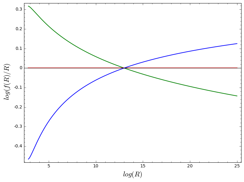
Figure 1: Plot of $f(R)/R$ against Ricci scalar $R$ for the early universe, setting $A=0.5$, $C_{2}=0$ and $C_{1}=-0.4$, the red is for GR case, green is for positive $f(R)$ solution and blue is for negative solution

Combining Eqs. (14) and (15) and use the fact that

$$\sqrt{A+\frac{B}{a^{6}}}=\frac{1}{a^{3}}\sqrt{B}\sqrt{1+\frac{Aa^{6}}{B}}\approx\frac{\sqrt{B}}{a^{3}}\;,$$ (32)

we obtain the potential $V(a)$ as

$$V(a)=\frac{\sqrt{B}}{a^{3}}\;.$$ (33)

We get $a(\phi)$ from Eq. (27) as

$$a^{3}=\frac{2\sqrt{B}}{\sqrt{A}(e^{\pm 2\sqrt{3}(\phi-C_{1})}-1)^{1/2}}\;.$$ (34)

Therefore, the potential is given as

$$V(\phi)=\frac{\sqrt{A}}{2}\Big{(}e^{\pm 2\sqrt{3}(\phi-C_{1})}-1\Big{)}^{\frac{1}{2}}\;.$$ (35)

We set the constants such that $V(\phi)$ is given as

$$V(\phi)=\frac{1}{2}\Big{(}e^{\pm 2\sqrt{3}\phi}-1\Big{)}^{\frac{1}{2}}\;.$$ (36)

Then the time-dependent potential can be obtained as

$$V(t)=\frac{\sqrt{B}}{D^{3}e^{3mt}}\;.$$ (37)

By considering positive potential from Eq. (36), one can write

$$V(\phi)=\frac{\sqrt{A}}{2}\Big{(}e^{2\sqrt{3}\phi}-1\Big{)}^{\frac{1}{2}}\;.$$ (38)

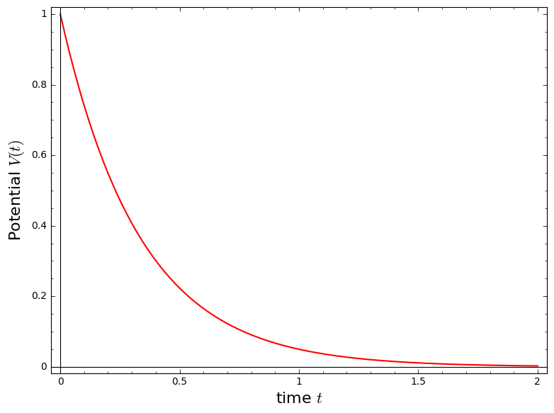
(a) The potential $V(t)$ as a function of time $t$ from Eq. (37) for values $A=B=m=D=1$ and $C=0.$

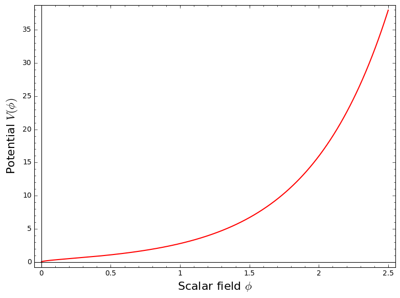
(b) The potential $V(\phi)$ as a function of the scalar field $\phi$ from Eq. (38) for values $A=B=m=D=1$ and $C=0.$

Figure 2:

3.2 Case 2: Late universe

The term on the denominator (20) can be approximated with the assumption that for the late universe, the scale factor $a$ is large enough such that $B/Aa^{6}<<1$ holds. Therefore, we have the term as

$$2\sqrt{ABa^{6}+B^{2}}=2\sqrt{ABa^{6}\Big{(}1+\frac{B}{Aa^{6}}\Big{)}}\approx 2\sqrt{AB}a^{3}\;.$$ (39)

With this approximation, equation (20) becomes

$$\phi(a)=\pm\frac{1}{2\sqrt{3}}\ln\Big{(}1+\frac{2B}{Aa^{6}}+\frac{2\sqrt{B}}{\sqrt{A}a^{3}}\Big{)}+C_{1}\;.$$ (40)

Therefore Eq. (40) takes the form

$$\phi(a)=\pm\frac{1}{2\sqrt{3}}\ln\Big{(}\frac{2\sqrt{B}}{\sqrt{A}a^{3}}\Big{)}+C_{1}\;,$$ (41)

Eq. (22) results in

$$a^{6}=\frac{\sqrt{B}}{\sqrt{R\sqrt{A}-4A}}\;,~{}~{}R\neq 4\sqrt{A}.$$ (42)

Therefore, we update Eq. (40) as

$$\phi(R)=\pm\frac{1}{2\sqrt{3}}\ln\Big{(}1+\frac{2}{\sqrt{A}}\sqrt{R\sqrt{A}-4A}\Big{)}+C_{1}\;.$$ (43)

Replacing Eq. (43) in Eq. (8), we have $f(R)$ as

$$\begin{split}f(R)&=\pm\Big{[}\frac{\sqrt{3}}{6}\Big{(}R-\frac{17\sqrt{A}}{4}\Big{)}\ln\Big{(}1+\frac{2\sqrt{R\sqrt{A}-4A}}{\sqrt{A}}\Big{)}+\frac{\sqrt{3}}{12}\sqrt{R\sqrt{A}-4A}+\Big{(}-\frac{\sqrt{3}}{12}+C_{1}\Big{)}R\\ &+\frac{19\sqrt{3A}}{48}\Big{]}+R+C_{3}\;,\end{split}$$ (44)

where $C_{3}$ is a constant of integration.

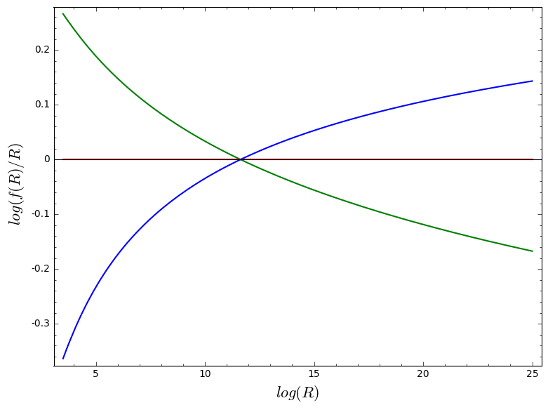
Figure 3: Plot of $f(R)/R$ against Ricci scalar $R$ for the late universe, setting $A=0.4$, $C_{3}=0$ and $C_{1}=-0.4$, the red line represents the GR case, while the green and blue curves depict negative and positive $f(R)$ solutions respectively

By combining Eqs. (14) and (15) and using the large-scale-factor approximation, we have the potential as

$$V(\phi)=\sqrt{A}\;.$$ (45)

As a combination of Eqs. (14) and (15) results in

$$V(a)=\frac{2A+\frac{B}{a^{6}}}{2\sqrt{A+\frac{B}{a^{6}}}}\;,$$ (46)

one can start from dependence of scale factor $a$ on scalar field $\phi$ to have the potential $V(\phi)$ as

$$V(\phi)=\frac{2A+\frac{A}{4}\Big{(}e^{\mp 2\sqrt{3}\phi-C_{1}}\Big{)}^{2}}{2\sqrt{A+\frac{A}{4}\Big{(}e^{\mp 2\sqrt{3}\phi-C_{1}}\Big{)}^{2}}}\;.$$ (47)

In principle, we can constrain the scalar field $\phi$ by equating Eqs. (45) and (47). Once this is done, one has a constant scalar field given by

$$\phi=\pm\frac{C_{1}}{2\sqrt{3}}\;.$$ (48)

So far, we have considered the original model of the Chaplygin gas and have obtained expressions for $f(R)$ that correspond to the early and late universe along with their corresponding potentials. In the following, we present a similar analysis for the generalized Chaplygin model.

4 Reconstruction of $f(R)$ gravity from the generalized Chaplygin gas model

For the generalized Chaplygin gas, we have the pressure as [30, 20, 16]

$$p=-\frac{A}{\mu^{\alpha}}\;,$$ (49)

where $0\leq\alpha\leq 1$ and $A$ is a constant.

$$\mu(a)=\Big{(}A+Ba^{-3(\alpha+1)}\Big{)}^{\frac{1}{1+\alpha}}\;.$$ (50)

For a flat universe, $K=0$, we can write the Friedmann equation as

$$\dot{a}=a\sqrt{\frac{\mu}{3}}\;.$$ (51)

Combining Eqs. (14) and (15) results in

$$\dot{\phi}^{2}=\frac{Ba^{-3(\alpha+1)}}{\Big{(}A+Ba^{-3(\alpha+1)}\Big{)}^{\frac{\alpha}{1+\alpha}}}\;.$$ (52)

Therefore, we can write

$$\phi^{\prime}=\pm\sqrt{\frac{3B}{Aa^{3\alpha+5}+Ba^{2}}}\;.$$ (53)

4.1 Case1: Early universe

We consider Eq. (53), for the early universe, the scale factor is assumed to be small enough, therefore, we can write

$$d\phi=\pm\frac{\sqrt{3B}}{\sqrt{Ba^{2}(1+\frac{Aa^{3(\alpha+1)}}{B})}}da\;,$$ (54)

then using the fact that $(1+x)^{n}\approx 1+nx+O(x^{2}),\text{ for }x<<1$, we have

$$d\phi=\pm\frac{\sqrt{3}}{a(1+\frac{Aa^{3(\alpha+1)}}{2B})}da\;.$$ (55)

Integrating this equation, we have

$$\phi(a)=\pm\frac{\sqrt{3}}{3(\alpha+1)}\ln\Big{(}\frac{2B}{a^{3(\alpha+1)}}+A\Big{)}+C_{1}\;.$$ (56)

By imposing the early universe assumption for scale factor on Eq. (72), we have $a(R)$ as

$$a(R)=\frac{B^{\frac{1}{3(\alpha+1)}}}{R^{1/3}}\;.$$ (57)

Therefore, we have $\phi(R)$ as

$$\phi(R)=\pm\frac{\sqrt{3}}{3(\alpha+1)}\ln(2R^{\alpha+1}+A)+C_{1}\;.$$ (58)

Thus integrating with respect to the Ricci scalar $R$ from

$$f(R)=\int\phi dR+R+C_{4}\;,$$ (59)

to have

$$f(R)=\pm\left[\frac{\sqrt{3}\Big{(}R(\alpha+1)-R\ln\left(2R^{\alpha+1}+A\right)\Big{)}}{3(\alpha+1)}-\frac{\sqrt{3}A}{3}\int\frac{dR}{2R^{\alpha+1}+A}+C_{1}R\right]+R+C_{4}\;,$$ (60)

where $C_{4}$ is a constant the integration.

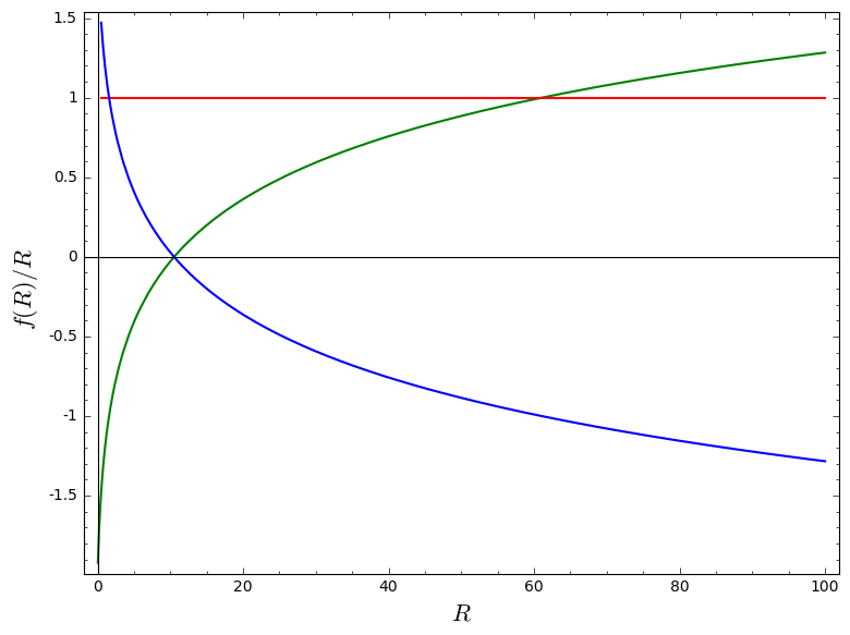
Figure 4: Plot of $f(R)/R$ against Ricci scalar $R$ for the early universe, setting $A=0$, $C_{4}=0$, $C_{1}=0.4$ and $\alpha=0.2$ the red line represents the GR case, while the green and blue curves depict negative and positive $f(R)$ solutions respectively

The potential is given by

$$V(\phi)=\frac{\mu_{\phi}-p_{\phi}}{2}\;.$$ (61)

Considering energy density as

$$\mu=\Big{(}A+Ba^{-3(\alpha+1)}\Big{)}^{\frac{1}{\alpha+1}}$$ (62)

and pressure as

$$p=-\frac{A}{\mu^{\alpha}}\;,$$ (63)

we have

$$V(a)=\frac{2A+\frac{B}{a^{3(\alpha+1)}}}{2(A+Ba^{-3(\alpha+1)})^{\alpha/(\alpha+1)}}\;.$$ (64)

By treating the denominator, we have

$$(A+Ba^{-3(\alpha+1)})^{\frac{\alpha}{(\alpha+1)}}=\Big{(}\frac{B}{a^{3(\alpha+1)}}(\frac{a^{3(\alpha+1)}}{B}+1)\Big{)}^{\frac{\alpha}{\alpha+1}}\approx\Big{(}\frac{B}{a^{3(\alpha+1)}}\Big{)}^{\frac{\alpha}{\alpha+1}}\;,$$ (65)

where we have considered that $a^{3(\alpha+1)}$ is small enough in the early universe. So the potential becomes

$$V(a)=\frac{2A+\frac{B}{a^{3(\alpha+1)}}}{2\Big{(}\frac{B}{a^{3(\alpha+1)}}\Big{)}^{\frac{\alpha}{\alpha+1}}}\;.$$ (66)

From Eq. (56), we have

$$a^{3(\alpha+1)}=\frac{2B}{e^{\mp\frac{3\phi(\alpha+1)}{\sqrt{3}}}-A}\;.$$ (67)

If we substitute (67) into (66), we get the potential $V$ as a function of $\phi$ as

$$V(\phi)=\frac{1}{2^{\frac{\alpha+2}{\alpha+1}}B}\Big{(}2A+\frac{1}{2}(e^{\pm\frac{3\phi(\alpha+1)}{\sqrt{3}}}-A)\Big{)}\Big{(}e^{\pm\frac{3\phi(\alpha+1)}{\sqrt{3}}}-A\Big{)}^{\frac{1}{\alpha+1}}\;.$$ (68)

We only consider positive potential as

$$V(\phi)=\frac{1}{2^{\frac{\alpha+2}{\alpha+1}}B}\Big{(}2A+\frac{1}{2}(e^{\frac{3\phi(\alpha+1)}{\sqrt{3}}}-A)\Big{)}\Big{(}e^{\frac{3\phi(\alpha+1)}{\sqrt{3}}}-A\Big{)}^{\frac{1}{\alpha+1}}\;.$$ (69)

Subsequently, Equations (66) and (25) give rise to

$$V(t)=\frac{1}{2B^{\frac{\alpha}{\alpha+1}}}\Big{(}2A+B(De^{mt})^{-3(\alpha+1)}\Big{)}(De^{mt})^{3\alpha}\;.$$ (70)

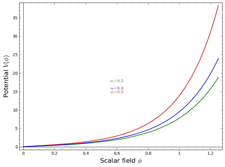
(a) The potential $V(\phi)$ as a function of scalar field $\phi$ from Eq. (69) for values $A=B=m=D=1$ and $\alpha=0.5$ (red), $\alpha=0.3$ (blue) and $\alpha=0.2$ (green).

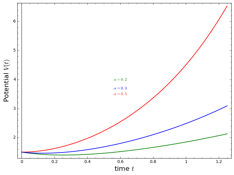
(b) The potential $V(t)$ as a function of time $t$ from Eq. (70) for values $A=B=m=D=1$ and $\alpha=0.5$ (red), $\alpha=0.3$ (blue) and $\alpha=0.2$ (green).

Figure 5:

4.2 Case2: Late universe

For the late universe, we have the following assumption

$$Ba^{2}<<Aa^{3\alpha+5}\;.$$ (71)

Thus we have

$$d\phi\approx\sqrt{\frac{3B}{Aa^{3\alpha+5}}}da\;.$$ (72)

We perform integration to get

$$\phi(a)=\pm\frac{2\sqrt{B}}{\sqrt{3}\sqrt{A}(\alpha+1)a^{3(\alpha+1)/2}}+C_{1}\;.$$ (73)

The next step is to get $\phi(R)$. Using the trace equation once again yields

$$R=\frac{Ba^{-3(\alpha+1)}+4A}{\Big{(}A+Ba^{-3(\alpha+1)}\Big{)}^{\frac{\alpha}{1+\alpha}}}\;.$$ (74)

By manipulating Eq. (74), we obtain

$$a(R)=\Big{(}\frac{RA^{\frac{\alpha}{1+\alpha}}-4A}{B(1-\frac{\alpha R}{1+\alpha}A^{\frac{-1}{\alpha+1}})}\Big{)}^{-\frac{1}{3(\alpha+1)}}\;.$$ (75)

Thus from Eq. (73), we have

$$\phi(R)=\pm\frac{2\sqrt{B}}{\sqrt{3A}(\alpha+1)}\Big{(}\frac{RA^{\frac{\alpha}{1+\alpha}}-4A}{B(1-\frac{\alpha R}{1+\alpha}A^{\frac{-1}{\alpha+1}})}\Big{)}^{\frac{1}{2}}\;.$$ (76)

Substituting this expression of $\phi(R)$ in Eq. (8), we get

$$\begin{split}f(R)=&\pm\Bigg{[}\frac{-A^{2}(3\alpha-1)^{2}m_{1}(A,\alpha,R)\arcsin\Big{(}\frac{2\alpha A\frac{\alpha}{\alpha+1}R-5A\alpha-A}{A(3\alpha-1)}\Big{)}+m_{2}(A,\alpha,R)}{4\sqrt{3}\alpha^{3/2}(\alpha+1)^{3/2}m_{1}(A,\alpha,R)}+C_{1}R\Bigg{]}\\ &+R+C_{5}\;,\end{split}$$ (77)

where $C_{5}$ is a constant of integration ,

$$m_{1}(A,\alpha,R)=\sqrt{-\alpha A^{\frac{\alpha}{\alpha+1}}\big{(}\alpha R-(\alpha+1)A^{\frac{1}{\alpha+1}}\big{)}\big{(}RA^{\frac{\alpha}{\alpha+1}}-4A\big{)}}\;,$$ (78)

and

$$\begin{split}m_{2}(A,\alpha,R)=&-4\alpha^{3}A^{\frac{3\alpha}{\alpha+1}}R^{3}+6(5\alpha+1)\alpha^{2}A^{\frac{3\alpha+1}{\alpha+1}}R^{2}-2\alpha(33\alpha^{2}+18\alpha+1)A^{\frac{3\alpha+2}{\alpha+1}}R\\ &+(40\alpha^{3}+48\alpha^{2}+18\alpha)A^{3}\;.\end{split}$$ (79)

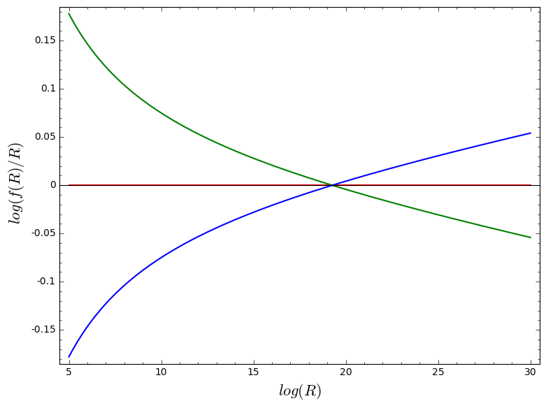
Figure 6: Plot of $f(R)/R$ against Ricci scalar $R$ for the late universe, setting $A=10^{-4}$, $C_{1}=-2\times 10^{-3}$, $C_{5}=1$ and $\alpha=3\times 10^{-5}$ the red line represents the GR case, while the green and blue curves depict negative and positive $f(R)$ solutions respectively

From Eq. (50) in late universe, that is together with its corresponding pressure, we have potential $V(a)$ from Eq. (23) as

$$V(a)=\frac{Ba^{-3(\alpha+1)}+A}{2\big{(}A+Ba^{-3(\alpha+1)}\big{)}^{\frac{\alpha}{\alpha+1}}}\;.$$ (80)

Replacing Eq. (73) in Eq. (80) we get

$$V(\phi)=\frac{3A(\alpha+1)^{2}\phi^{2}+8AB}{8B(A+3A(\alpha+1)^{2}\phi^{2})^{\frac{\alpha}{\alpha+1}}}\;.$$ (81)

We replace scale factor (25) in (80) to get potential as a function of time as

$$V(t)=\frac{B(De^{mt})^{-3(\alpha+1)}+2A}{2\big{(}A+B(De^{mt})^{-3(\alpha+1)}\big{)}^{\frac{\alpha}{\alpha+1}}}\;.$$ (82)

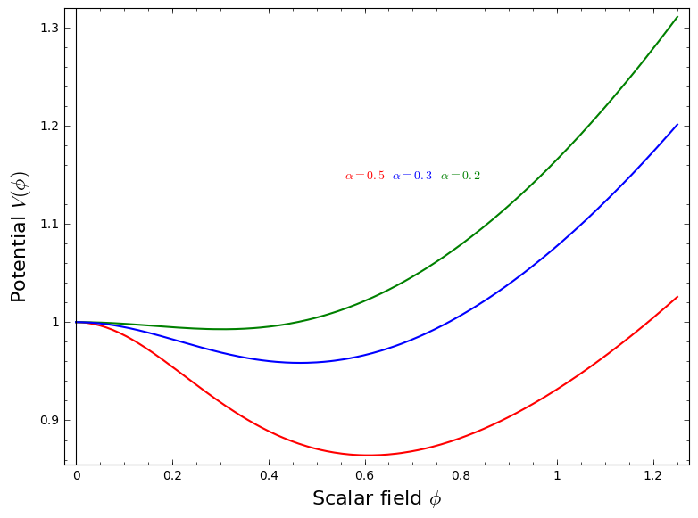
(a) The potential $V(\phi)$ as a function of scalar field $\phi$ from Eq. (81) for values $A=B=m=D=1$, and $\alpha=0.5$ (red), $\alpha=0.3$ (blue) and $\alpha=0.2$ (green).

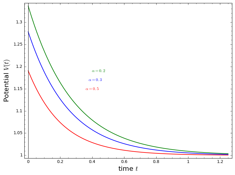
(b) The potential $V(t)$ as a function of time $t$ from Eq. (82) for values $A=B=m=D=1$, and $\alpha=0.5$ (red), $\alpha=0.3$ (blue) and $\alpha=0.2$ (green).

Figure 7:

For the early universe, we plotted the potential dependence on the scalar field and one can easily observe that the potential increases with an increase in $\phi$. However, for the late universe, this dependence is realized after a decrease to a certain minimum. It can be observed that as $\alpha$ increases the position of the minimum point gets lowered. For the time-dependent potential in the early universe, an increase in time results in an increase in the potential. Conversely, the potential decreases as time increases for the late universe. This trend has been obtained through the use of approximated solutions. The actual behavior of the potential under consideration may be obtained through acquiring the exact solutions of the scalar field.

5 Conclusions

The reconstruction of $f(R)$ models from the Chaplygin gas cosmological model is systematically developed in this work. This was done through the consideration of the equivalence between two theories of gravitation, namely $f(R)$ theory and the Brans-Dicke subclass of scalar-tensor models. The analysis made use of a combination of energy density, pressure, kinetic and potential terms of the scalar field to obtain relationships between the scalar field, the Ricci scalar and the scale factor. As can be seen from the reconstructed functionals and their corresponding plots versus the GR Lagrangian density ($f(R)=R)$, these expressions have GR as their respective limiting solutions.

The results have been applied to a de Sitter universe and the time-dependent expressions for the potential have been obtained for both the original and generalized cases of the Chaplygin gas model. This was made possible by two asymptotic assumptions, early- and late-universe epochs of cosmic evolution. The behaviors of the potential for both the original and generalized cases show that the amplitude of the potential gets weaker with time in a de Sitter universe except for the early universe consideration in the generalized Chaplygin gas model where the potential grows with time. However, the dependence of the potential on the scalar field shows that for larger values of the scalar field, the potential is also large, but for the generalized case within a late universe, the potential is observed to have a valley before it follows the trend observed for other potentials.

The solutions provided in this work are obtained for asymptotic cases, but intermediate solutions are highly intractable at best. We thus leave the (numerical) analysis of solutions for the entire cosmic history for a future work.

References

- [1] Marek Kowalski, David Rubin, Greg Aldering, RJ Agostinho, A Amadon, R Amanullah, C Balland, K Barbary, G Blanc, PJ Challis, et al. Improved cosmological constraints from new, old, and combined supernova data sets. The Astrophysical Journal, 686(2):749, 2008.
- [2] Alexei A Starobinsky. A new type of isotropic cosmological models without singularity. Physics Letters B, 91(1):99–102, 1980.
- [3] Katsuhiko Sato. First-order phase transition of a vacuum and the expansion of the universe. Monthly Notices of the Royal Astronomical Society, 195(3):467–479, 1981.
- [4] Demosthenes Kazanas. Dynamics of the universe and spontaneous symmetry breaking. The Astrophysical Journal, 241:L59–L63, 1980.
- [5] Andrew R Liddle and David H Lyth. Cosmological inflation and large-scale structure. Cambridge University Press, 2000.
- [6] George F Smoot, CL Bennett, A Kogut, EL Wright, J Aymon, NW Boggess, ES Cheng, G De Amici, S Gulkis, MG Hauser, et al. Structure in the COBE differential microwave radiometer first-year maps. The Astrophysical Journal, 396:L1–L5, 1992.
- [7] Adam G Riess, Alexei V Filippenko, Peter Challis, Alejandro Clocchiatti, Alan Diercks, Peter M Garnavich, Ron L Gilliland, Craig J Hogan, Saurabh Jha, Robert P Kirshner, et al. Observational evidence from supernovae for an accelerating universe and a cosmological constant. The Astronomical Journal, 116(3):1009, 1998.
- [8] Varun Sahni and Alexei Starobinsky. The case for a positive cosmological -term. International Journal of Modern Physics D, 9(04):373–443, 2000.
- [9] Saurabh Jha, Robert P Kirshner, Peter Challis, Peter M Garnavich, Thomas Matheson, Alicia M Soderberg, Genevieve JM Graves, Malcolm Hicken, Joao F Alves, Héctor G Arce, et al. UBVRI light curves of 44 type Ia supernovae. The Astronomical Journal, 131(1):527, 2006.
- [10] Max Tegmark, Michael A Strauss, Michael R Blanton, Kevork Abazajian, Scott Dodelson, Havard Sandvik, Xiaomin Wang, David H Weinberg, Idit Zehavi, Neta A Bahcall, et al. Cosmological parameters from SDSS and WMAP. Physical Review D, 69(10):103501, 2004.
- [11] Max Tegmark, Daniel J Eisenstein, Michael A Strauss, David H Weinberg, Michael R Blanton, Joshua A Frieman, Masataka Fukugita, James E Gunn, Andrew JS Hamilton, Gillian R Knapp, et al. Cosmological constraints from the SDSS luminous red galaxies. Physical Review D, 74(12):123507, 2006.
- [12] Will J Percival, Shaun Cole, Daniel J Eisenstein, Robert C Nichol, John A Peacock, Adrian C Pope, and Alexander S Szalay. Measuring the baryon acoustic oscillation scale using the Sloan Digital Sky Survey and 2df galaxy redshift survey. Monthly Notices of the Royal Astronomical Society, 381(3):1053–1066, 2007.
- [13] E. Komatsu, J. Dunkley, M. R. Nolta, C. L. Bennett, B. Gold, G. Hinshaw, N. Jarosik, D. Larson, M. Limon, L. Page, D. N. Spergel, M. Halpern, R. S. Hill, A. Kogut, S. S. Meyer, G. S. Tucker, J. L. Weiland, E. Wollack, and E. L. Wright. Five-year Wilkinson Microwave Anisotropy Probe observations: Cosmological interpretation. The Astrophysical Journal Supplement Series, 180(2):330.
- [14] Surajit Chattopadhyay and Ujjal Debnath. Interaction between phantom field and modified Chaplygin gas. Astrophysics and Space Science, 326(2):155–158, 2010.
- [15] MC Bento, O Bertolami, and AA Sen. Generalized Chaplygin gas, accelerated expansion, and dark-energy-matter unification. Physical Review D, 66(4):043507, 2002.
- [16] V Gorini, A Kamenshchik, U Moschella, and V Pasquier. The Chaplygin gas as a model for dark energy. 20:26, 2003.
- [17] Abha Dev, JS Alcaniz, and Deepak Jain. Cosmological consequences of a Chaplygin gas dark energy. Physical Review D, 67(2):023515, 2003.
- [18] Alexander Kamenshchik, Ugo Moschella, and Vincent Pasquier. An alternative to quintessence. Physics Letters B, 511(2).
- [19] Neven Bilić, Gary B Tupper, and Raoul D Viollier. Unification of dark matter and dark energy: the inhomogeneous Chaplygin gas. Physics Letters B, 535(1):17–21, 2002.
- [20] Vittorio Gorini, Alexander Kamenshchik, and Ugo Moschella. Can the Chaplygin gas be a plausible model for dark energy? Physical Review D, 67(6):063509, 2003.
- [21] HB Benaoum. Modified Chaplygin gas cosmology. Advances in High Energy Physics, 2012, 2012.
- [22] SM Carroll, V Duvvuri, MS Turner, and M Trodden. Is cosmic speed-up due to new gravitational physics? Physical Review D, 70(4):043528.
- [23] Salvatore Capozziello, VF Cardone, and A Troisi. Dark energy and dark matter as curvature effects? Journal of Cosmology and Astroparticle Physics, 2006(08):001, 2006.
- [24] Salvatore Capozziello and Mariafelicia De Laurentis. Extended theories of gravity. Physics Reports, 509(4):167–321, 2011.
- [25] ShinOichi Nojiri and Sergei D Odintsov. Unified cosmic history in modified gravity: from theory to Lorentz non-invariant models. Physics Reports, 505(2):59–144, 2011.
- [26] Shin’ichi Nojiri, SD Odintsov, and D Sáez-Gómez. Cyclic, ekpyrotic and little rip universe in modified gravity. In Towards new paradigms: Proceeding of the Spanish relativity meeting 2011, volume 1458, pages 207–221. AIP Publishing, 2012.
- [27] Shin’Ichi Nojiri and Sergei D Odintsov. Introduction to modified gravity and gravitational alternative for dark energy. International Journal of Geometric Methods in Modern Physics, 4(01):115–145, 2007.
- [28] Thomas P Sotiriou and Valerio Faraoni. theories of gravity. Reviews of Modern Physics, 82(1):451, 2010.
- [29] Timothy Clifton, Pedro G Ferreira, Antonio Padilla, and Constantinos Skordis. Modified gravity and cosmology. Physics Reports, 513(1):1–189, 2012.
- [30] Maye Elmardi, Amare Abebe, and Abiy Tekola. Chaplygin-gas solutions of Gravity. International Journal of Geometric Methods in Modern Physics, 13:1650120, 2016.
- [31] Shin’Ichi Nojiri and Sergei D Odintsov. Modified gravity with negative and positive powers of curvature: Unification of inflation and cosmic acceleration. Physical Review D, 68(12):123512, 2003.
- [32] Shin’ichi Nojiri and Sergei D Odintsov. Unifying inflation with CDM epoch in modified gravity consistent with solar system tests. Physics Letters B, 657(4):238–245, 2007.
- [33] Yong-Seon Song, Wayne Hu, and Ignacy Sawicki. Large scale structure of gravity. Physical Review D, 75(4):044004, 2007.
- [34] Amare Abebe, Álvaro de la Cruz-Dombriz, and Peter KS Dunsby. Large scale structure constraints for a class of theories of gravity. Physical Review D, 88(4):044050, 2013.
- [35] A de La Cruz-Dombriz, A Dobado, and AL Maroto. Evolution of density perturbations in theories of gravity. Physical Review D, 77(12):123515, 2008.
- [36] S Carloni, PKS Dunsby, and A Troisi. Evolution of density perturbations in gravity. Physical Review D, 77(2):024024, 2008.
- [37] Kishore N Ananda, Sante Carloni, and Peter KS Dunsby. Structure growth in theories of gravity with a dust equation of state. Classical and Quantum Gravity, 26(23):235018, 2009.
- [38] Amare Abebe and Maye Elmardi. Irrotational-fluid cosmologies in fourth-order gravity. International Journal of Geometric Methods in Modern Physics, 12(10):1550118, 2015.
- [39] Amare Abebe, Peter KS Dunsby, and Deon Solomons. Integrability conditions of quasi-newtonian cosmologies in modified gravity. International Journal of Modern Physics D, page 1750054, 2016.
- [40] Amare Abebe. Anti-newtonian cosmologies in gravity. Classical and Quantum Gravity, 31(11):115011, 2014.
- [41] Amare Abebe, Davood Momeni, and Ratbay Myrzakulov. Shear-free anisotropic cosmological models in gravity. General Relativity and Gravitation, 48(4):1–17, 2016.
- [42] Salvatore Capozziello and Mauro Francaviglia. Extended theories of gravity and their cosmological and astrophysical applications. General Relativity and Gravitation, 40(2):357–420, 2008.
- [43] Alvaro de la Cruz-Dombriz. Some cosmological and astrophysical aspects of modified gravity theories. arXiv preprint arXiv:1004.5052, 2010.
- [44] Takeshi Chiba, Tristan L Smith, and Adrienne L Erickcek. Solar system constraints to general gravity. Physical Review D, 75(12):124014, 2007.
- [45] Miguel Aparicio Resco, Álvaro de la Cruz-Dombriz, Felipe J Llanes Estrada, and Víctor Zapatero Castrillo. On neutron stars in theories: small radii, large masses and large energy emitted in a merger. Physics of the Dark Universe, 13:147–161, 2016.
- [46] Thomas P Sotiriou. gravity and scalar–tensor theory. Classical and Quantum Gravity, 23(17):5117, 2006.
- [47] Valerio Faraoni. de sitter space and the equivalence between and scalar-tensor gravity. Physical Review D, 75(6):067302, 2007.
- [48] Thomas Faulkner, Max Tegmark, Emory F Bunn, and Yi Mao. Constraining gravity as a scalar-tensor theory. Physical Review D, 76(6):063505, 2007.
- [49] Joseph Ntahompagaze, Amare Abebe, and Manasse Mbonye. On gravity in scalar–tensor theories. International Journal of Geometric Methods in Modern Physics, page 1750107, 2017.
- [50] Thomas P Sotiriou and Valerio Faraoni. theories of gravity. Reviews of Modern Physics, 82(1):451, 2010.
- [51] Amare Abebe. Beyond Concordance Cosmology. Scholars Press, 2015.
- [52] Andrei V Frolov. Singularity problem with models for dark energy. Physical review letters, 101(6):061103, 2008.
- [53] Timothy Clifton, Pedro G Ferreira, Antonio Padilla, and Constantinos Skordis. Modified gravity and cosmology. Physics Reports, 513(1):1–189, 2012.
- [54] Gonzalo J Olmo. Post-newtonian constraints on cosmologies in metric and palatini formalism. Physical Review D, 72(8):083505, 2005.
- [55] GFR Ellis and MS Madsen. Exact scalar field cosmologies. Classical and Quantum Gravity, 8(4):667, 1991.
- [56] Vicenç Méndez. Exact scalar field cosmologies with a fluid. Classical and Quantum Gravity, 13(12):3229, 1996.