The topography of the environment alters the optimal search strategy for active particles
Abstract
In environments with scarce resources, adopting the right search strategy can make the difference between succeeding and failing, even between life and death. At different scales, this applies to molecular encounters in the cell cytoplasm, to animals looking for food or mates in natural landscapes, to rescuers during search-and-rescue operations in disaster zones, and to genetic computer algorithms exploring parameter spaces. When looking for sparse targets in a homogeneous environment, a combination of ballistic and diffusive steps is considered optimal; in particular, more ballistic Lévy flights with exponent are generally believed to optimize the search process. However, most search spaces present complex topographies. What is the best search strategy in these more realistic scenarios? Here we show that the topography of the environment significantly alters the optimal search strategy towards less ballistic and more Brownian strategies. We consider an active particle performing a blind cruise search for non-regenerating sparse targets in a two-dimensional space with steps drawn from a Lévy distribution with exponent varying from to (Brownian). We demonstrate that, when boundaries, barriers and obstacles are present, the optimal search strategy depends on the topography of the environment with assuming intermediate values in the whole range under consideration. We interpret these findings using simple scaling arguments and discuss their robustness to varying searcher’s size. Our results are relevant for search problems at different length scales, from animal and human foraging, to microswimmers’ taxis, to biochemical rates of reaction.
Introduction
What is the best strategy to search for randomly located resources? This is a crucial question for fields as diverse as biology, genetics, ecology, anthropology, soft matter, computer sciences and robotics BenichouRMP2011 ; ViswanathanBook2011 . In order to describe and analyse how a searcher browses the search space, many different plausible models have been proposed, including Brownian motion, intermittent search patterns, as well as Lévy flights and walks BenichouRMP2011 ; ViswanathanBook2011 ; Shlesinger1986 . In particular, Lévy statistics, among others models BenichouRMP2011 , have been successfully used to describe the emergence of optimal search strategies in natural systems at different length scales, from molecular entities LomholtPRL2005 ; ChenNatMat2015 , to swimming and swarming microorganisms ArielNatCom2015 ; KorobkovaNature2004 ; TuPRL2005 , to crawling eukaryotic cells HarrisNature2012 , to different species of foraging animals ViswanathanNature1996 ; ViswanathanNature1999 ; AtkinsonOikos2002 ; Ramos-FernandezBES2004 ; SimsNature2008 ; HumphriesNature2010 ; JagerScience2011 , to human motion patterns BrockmannNature2006 ; GonzalezNature2008 ; RaichlenPNAS2014 , although in the field of movement ecology there is some controversy on how universal Lévy searches are EdwardsNature2007 ; MashanovaJRSI2010 ; Petrovskii2PNAS2011 ; HumphriesPNAS2012 ; JansenScience2012 ; ReynoldsPLR2015 . Lévy statistics have also found applications in science and engineering, e.g., for defining the optimal search strategy for robots DartelCS2004 and for describing anomalous diffusion and navigation on networks RiascosPRE2012 ; GuoSciRep2016 .
The strategies based on Lévy statistics can be described under a unified framework where the searcher is an active particle BechingerRMP2016 that performs random jumps (blind search) whose lengths are drawn from a stable distribution . The two limiting cases for and correspond to ballistic and Brownian motion, respectively. The intermediate cases combine diffusive (i.e. local exploration) and ballistic (i.e. decorrelating, long-range excursions) steps in different proportions. In particular, the case for corresponds to a compromise superdiffusive regime, where the searcher explores its surroundings while reducing oversampling compared with a pure Brownian strategy ViswanathanNature1999 ; LomholtPNAS2008 ; ViswanathanBook2011 . When resources are plentiful, the most efficient strategy is a Brownian search ()ViswanathanNature1999 ; SimsNature2008 ; HumphriesNature2010 ; when resources are sparse, however, a Lévy strategy with performs better over a pure Brownian strategy ViswanathanBook2011 . In general, more ballistic search strategies (i.e. ) have been shown to be optimal in a wide range of situations, with the specific value of the exponent dependent on, e.g., the nature of the encounters with the targets (i.e. destructive or non-destructive) or the presence of memory in the searcher’s motion ViswanathanNature1999 ; BartumeusPRL2002 ; RaposoPRL2003 ; JamesPRE2008 ; RaposoPLOS2011 ; HumphriesPNAS2012 ; FerreiraPhysicaA2012 .
These studies have limited their analysis to landscapes characterized by a barrier-free homogenous topography. However, in realistic scenarios the environment is often characterized by a more complex topography, where boundaries, barriers and obstacles play a crucial role in determining the searcher’s motion. Examples of complex search spaces include cytoplasm for molecules within cells BarkayPhysToday2012 , biological tissue (or soil) for motile bacteria KimNatMicrobiol2016 , and patchy landscapes for foraging animals BoyerPRSLB2006 . This complexity can significantly influence the long-term behaviour of the system under study PinceNatCom2016 . As it has been recently shown, even a small perturbation, such as an external drift, can shift the optimal search strategy towards more Brownian strategies PalyulinPNAS2014 .
Here, by considering a searcher performing a blind cruise search for uniformly distributed non-regenerating sparse targets, we show with numerical simulations and simple scaling arguments that the exponent that optimizes the search strategy depends on the topography of the environment. In particular, we show that, differently from the homogeneous case where typically optimizes the search process, the optimal search strategy tends towards less ballistic and more Brownian cases, corresponding to values for the exponent in the range .
Results
Search in a homogenous topography
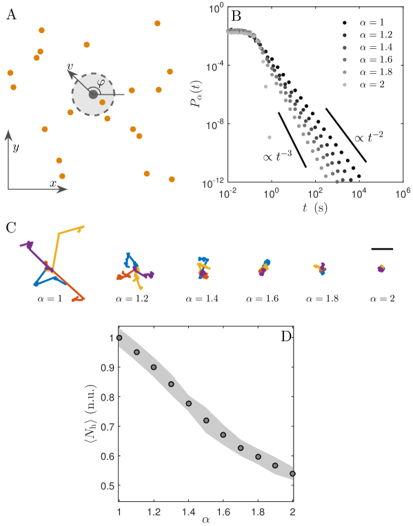
We start by analyzing an active particle of radius blindly searching for targets in an environment with a homogeneous topography, i.e. without any physical obstacles. As the active particle cruises the search space, it continuously captures the targets that come within a capture radius from its center, as schematically shown in Fig. 1A. The number of targets caught in each run is proportional to the area swept by the capture region surrounding the active particle. We assume the targets to be uniformly distributed, non-regenerating and scarce, i.e. with density . The latter condition implies that, once an active particle captures a target, the probability of finding a second one is negligible if the particle moves by .
The active particle performs a run-and-tumble motion, i.e. it has a fixed speed and changes its orientation by a normally-distributed angle with zero mean and standard deviation at discrete time intervals with BechingerRMP2016 . In the following, we set and . The time intervals between changes of direction are drawn from a Lévy distribution of exponent (Fig. 1B) ViswanathanBook2011 . Asymptotically, this distribution tends to a power law with exponent for ViswanathanBook2011 :
| (1) |
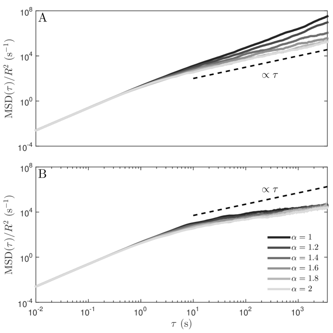
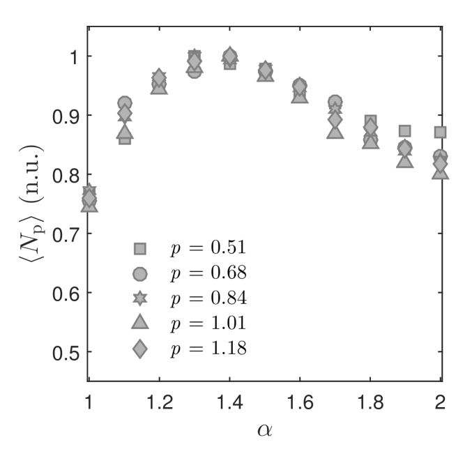
where is a normalization constant such that ; for the distribution is a Gaussian which decays exponentially in . As is constant, the run lengths are also distributed according to a Lévy distribution of same index , thus leading the particle to move superdiffusively for and diffusively for at long times (Fig. S1A)ViswanathanBook2011 . Examples of trajectories for various values of are shown in Fig. 1C: as decreases from the case of a pure Brownian strategy (), the searchers tend to move ballistically over longer distances before a change in orientation occurs. These different superdiffusive regimes allow the searcher to explore the overall search space combining ballistic and diffusive steps in different proportions ViswanathanNature1999 ; LomholtPNAS2008 ; ViswanathanBook2011 . Figure 1D plots the average number of caught targets obtained from 1000 simulated 1-hour trajectories as a function of . This number decreases as a function of , so that the optimal search strategy is for while the worst is the Brownian (), in agreement with foraging theory ViswanathanBook2011 .
Search in a porous topography
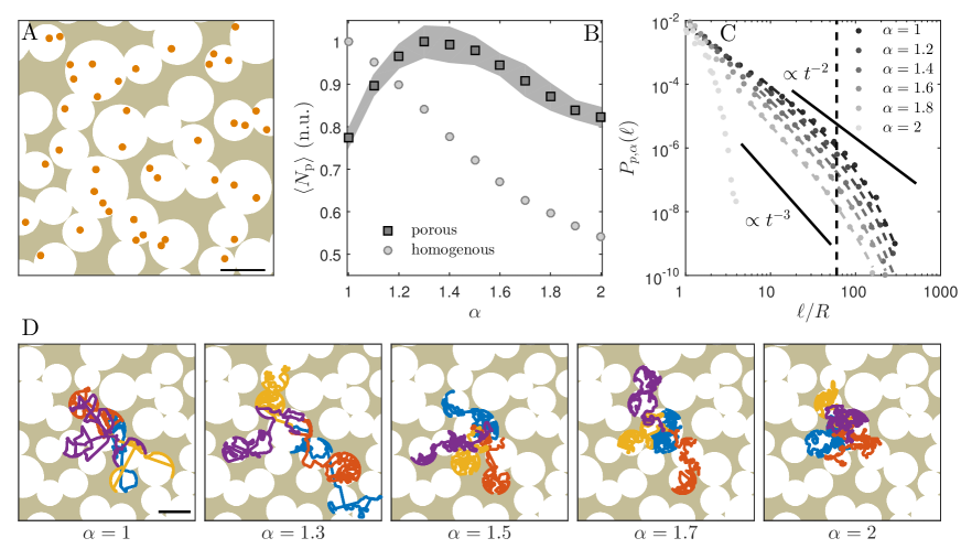
In order to understand how the complexity of the environment influences the optimal search strategy, we now consider an active particle looking for targets in a medium with a heterogenous topography (Fig. 2A). Specifically, the search space is now a two-dimensional porous medium constituted by uniformly distributed circular interconnected pores with average radius ; the characteristic size of a cluster of pores is much bigger than the total particle’s displacement within the simulation time. We model the interaction with the pore walls using reflective boundary conditions so that the particle moves along the walls until its orientation changes to point away from the boundary VolpeAJP2014 . This scenario is realistic at different length scales as indeed both biological and artificial microswimmers and elementary robots behave in a similar way BechingerRMP2016 ; DimidovANTS2016 .
As it can be seen in Fig. 2B, moving in such a porous environment shifts the optimal search strategy towards a more Brownian strategy () from the more ballistic case in the homogenous topography (). This shift can be understood in quantitative terms by looking at the effective probability distribution of the run lengths in the porous medium (Fig. 2C). This distribution is well-approximated by a power law with an exponential cutoff at
| (2) |
where is a normalization constant such that and is a proportionality constant; is estimated by fitting the previous function to the simulated data and, in general, depends on the geometrical features of the medium. As a result of this interaction with the boundaries, therefore, the porosity affects longer run lengths more than shorter ones, thus mainly penalizing the more ballistic strategies over the more Brownian ones. In other terms, even if the changes in the particle’s orientation are still dictated by the distributions in Fig. 1B, the boundaries effectively limit the maximum run length leading the particles to perform a subdiffusive motion rather than a superdiffusive one as in the homogenous environment (Fig. S1B); this behavior is in accordance with observations on persistent random walkers in the presence of obstacles ChepizhkoPRL2013sub . Qualitatively, this can also be appreciated by looking at some sample trajectories for different values of (Fig. 2D): when decreases, the particles tend to spend longer portions of their trajectories at the walls, thus exploring less efficiently the inner area of the pores. It is interesting to note that, at least when the searcher explores the complex topography for a finite time as in our simulations, the average shift in the optimal search strategy depends on the pore characteristic size, while it is largely independent of the density of pores and the local configuration of the explored cluster (Fig. S2).
Scaling arguments
In order to formalize the shift in the optimal search strategy due to the topography of the environment, we define the efficiency of catching targets in the porous medium compared to the homogeneous case as
| (3) |
Since the mean square displacement of the active particle is of order in a homogenous topography, self-intersections constitute a negligible fraction of the overall path for , which is closely related to the fact that the Hausdorff dimension of a Lévy process in the plane is equal to its exponent blumenthal1960dimension ; this is also the case in the porous topography for run lengths just below the spatial cutoff (Fig. 2C), which contribute with higher probability to the capture of new targets. As a consequence, to a first approximation, we obtain that the target capture rate is proportional to the average step length for a given topography and a given , so that
| (4) |
where is a function of the particle speed, is a constant, , , and and are the average step lengths in the porous and homogenous topography respectively (see Methods for their calculation).
While Eq. 4 explicitly depends on the particle’s speed through , the normalized efficiency defined as
| (5) |
is a universal curve that does not directly depend on . Interestingly, from this equation, the geometrical meaning of is apparent as the percentage of time that the particle spends running instead of being stuck at a boundary above the spatial cutoff .
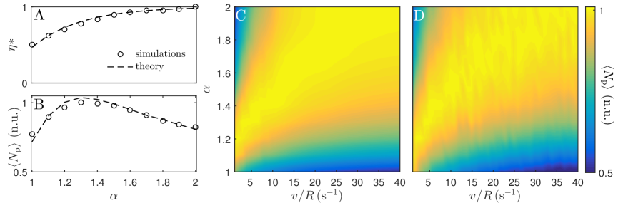
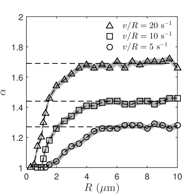
Using Eq. 5, we can therefore estimate the shift in the optimal search strategy due to the topography of the environment by finding the maximum of , i.e. only based on geometrical parameters (, and ) and the knowledge of the particle’s behavior in a homogenous topography . As it can be seen in Fig. 3A, Eq. 5 reproduces very well the simulated data, being the only fitting parameter in our case, and allows us to predict correctly the optimal value for the capture rate in the porous medium from (Fig. 3B). By comparing model predictions (Fig. 3C) with simulated data (Fig. 3D), Figs. 3C-D show how, once is known, this simple model based on scaling arguments predicts correctly the optimal strategy in the porous medium at any particle speed. These figures show that, for a given , the speed at which the particle moves within the environment has also an effect on the optimal search strategy: for low values of speed, the optimal search strategy shifts towards the more ballistic case (), as the particle tends to interact with the boundaries only at very long times, thus mostly moving as in an effectively homogenous environment; however, when increases, the optimal search strategy shifts more and more towards the Brownian case (), since this case is the one that minimizes the interaction with the boundaries over time.
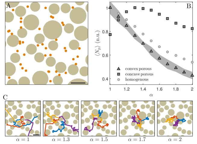
For further confirmation of the fact that the shift in optimal search strategy is due to the upper spatial cutoff introduced by the topography of the environment, we now consider a porous medium with a convex topography instead of the concave topography considered previously (Fig. 2A). In this topography, the particle searches for uniformly distributed targets within an interconnected space containing convex obstacles where there is no upper cutoff, i.e. (Fig. 4A). Also in this case the average radius of the obstacles is chosen so that . As expected, the optimal search strategy remains at (Fig. 4B), as for a particle searching in a homogenous space (Fig. 1D). In qualitative terms, these results can be interpreted by observing sample trajectories for various values of (Fig. 4C): in fact, as it can be appreciated from these trajectories, the convex porosity does not prevent the particles from moving ballistically over long distances when the value of is decreased.
Search in the presence of Brownian diffusion
The results shown so far apply to most length scales as long as properly rescaled to the particle’s radius . However, when approaches the micro- and nanoscale, Brownian diffusion starts playing a significant role in the translational and rotational motion of an active particle BechingerRMP2016 ; VolpeAJP2014 . In particular, while the translational diffusion of a particle scales with its inverse linear dimension (), its rotational diffusion scales with its inverse volume (). As a consequence of this volumetric scaling, as decreases, Brownian rotation randomizes any persistence in the particle’s orientation due to the Lévy strategy. Brownian diffusion becomes then an important parameter to consider when determining the optimal search strategy in a non-trivial topography for microscopic active particles, such as biological and artificial microswimmers (e.g. motile bacteria ArielNatCom2015 ; KorobkovaNature2004 ; TuPRL2005 and manmade micro- and nanorobots BechingerPRE2016 ) moving in complex and disordered environments ChepizhkoPRL2013 ; ReichhardtPRE2014 ; PinceNatCom2016 ; BechingerRMP2016 . Fig. 5A shows how the optimal search strategy (i.e. the optimal value of ) varies as a function of the particle’s radius, i.e. of the strength of the particle’s translational and rotational Brownian diffusion coefficients. We focus again on the environment of Fig. 2A, as it shows a clear deviation from the homogenous case (Fig. 1). For a given (e.g. for ), when is above a certain threshold value (e.g. for , corresponding to a sufficiently weak rotational diffusion), the optimal strategy is the same as the one predicted in Fig. 3C (Fig. 5A and 5B). However, when decreases (entailing a stronger rotational diffusion), the optimal search strategy shifts towards (Fig. 5A and 5C). This shift happens because the increased rotational diffusion leads to a reduction of the time that the particle spends at the boundaries. This effectively reduces the penalization that boundaries have on more ballistic strategies, thus allowing for the exploration of a greater inner area of the porous structure compared to more diffusive strategies. Reducing further, the optimal search strategy remains at although the relative efficiency over other values decreases (Fig. 5D). Finally, for even smaller values of (e.g. for ), the search process becomes effectively insensitive to the value of (Fig. 5E), as the increase in rotational diffusion makes persistent motion negligible BechingerRMP2016 .
Discussion
Our results demonstrate the critical role played by the topography of the environment in determining the optimal search strategy for an active particle whose run lengths are drawn from a Lévy distribution. In particular, the presence of physical boundaries, barriers and obstacles can introduce a cutoff on the distribution of steps that can penalize more ballistic strategies over more Brownian ones depending on different geometrical parameters connected to the topography of the environment and its interaction with the particle’s motion.
In our model, we assumed that the particle is performing a cruise search with continuous visibility for targets and perfect hitting probabilities. While we do not expect imperfect hitting probabilities to affect the optimality of the search strategy in our case as long as they affect all values equally, other search scenarios might influence the optimal search strategy in a complex topography BenichouRMP2011 : for example, in the case of intermittent search strategies, where there is an alternation between phases of slow motion that allow the searcher to detect the targets and phases of fast motion during which targets cannot be detected; or in the case of a search strategy with in-built delays so that, after a target is caught, some time must elapse before the following target can be caught.
Another aspect that can influence the optimal search strategy is the interaction between the searcher and the obstacles encoded in the boundary conditions. In this work, we have implemented reflective boundary conditions, which implies that the searcher stays at the boundary until a random reorientation event makes it point away from the obstacle. This scenario is realistic at the macroscopic and microscopic scale, as for example both elementary robots and microswimmers (biological and non) have been reported to behave in this way DimidovANTS2016 ; BechingerRMP2016 . Alternatively, different responses can be considered in the presence of boundaries, when information obtained from sensing the surroundings for example leads to a voluntary switch in the strategy adopted by the searcher.
As the search time is generally a limiting factor in many realistic search scenarios BenichouRMP2011 , the searcher was allowed to explore the search space for a finite time in our simulations. Nevertheless, from a fundamental point of view, it would be interesting to study how the optimal search strategy is influenced by the topography of the environment in the limit of infinite search times. In the case of infinite searches, interesting behaviors could emerge as a result of the interplay between the fractal dimensionality of the searcher’s trajectory and that of the environment in a porous topography at the percolation threshold or in a network of channels.
Our findings are mostly scale-invariant and only partially break down at the nanoscopic scale () when rotational diffusion becomes predominant. One important implication of this is that different search strategies (i.e. different values of ) will lead to similar outcomes for nanoscopic particles such as biomolecules and molecular motors moving in a two-dimensional space (Fig. 5E). This issue can be overcome by reducing the dimensionality of the environment, for example by introducing a preferential direction of motion with molecular rails. In fact, Lévy-type statistics emerge for molecular motors performing searches on polymer chains such as DNA LomholtPRL2005 , or on one-dimensional molecular rails such as microtubules ChenNatMat2015 . Similarly, increasing the dimensionality of the system to a three-dimensional space will alter the probability that the searcher goes back to the same point compared to a two-dimensional space, and thus its optimal search strategy in a complex three-dimensional environment can also be affected.
Our results are relevant for all random search problems where the searcher explores complex search spaces. Examples at various length scales include the rate of molecular encounters in the cytoplasm of cells, the localization of nutrients by motile bacteria in tissue or soil, the foraging of animals in patchy landscapes as well as search-and-rescue operations in ruins following natural disasters. Furthermore, similar dynamics could also be applied to optimize navigation in topologically complex networks RiascosPRE2012 ; GuoSciRep2016 .
Materials and Methods
Numerical simulations
In our numerical model, we consider active particles of radius performing a two-dimensional run-and-tumble motion according to the following equations:
where is the particle’s position, is the particle’s speed, and is the particle’s orientation during the -th time interval where . The time intervals between changes of direction are drawn from a Lévy distribution of exponent ; only the absolute value of the number is considered. At the end of each time interval the particle orientation changes by a random angle according to a normal distribution with zero mean and standard deviation . The initial position for the trajectory was randomly chosen within the medium according to a uniform distribution. The positions of the targets were randomized for each trajectory. Interactions with the walls were modeled using the boundaries conditions described in Ref. VolpeAJP2014 . In the data in Fig. 5, translational and rotational Brownian motion are included by adding three independent white noise processes ( , and ) to the equations of motion VolpeAJP2014 ; in this set of simulations, the active particles are moving in an aqueous environment (, ).
Calculation of the average run length
In a homogenous topography
The average run length in a homogenous environment is
where represents the time that it takes for an active particle to travel a distance equal to its capture radius . Neglecting the first integral because it gives a small contribution to the average run length, we obtain
which, using the asymptotic analytical form for in Eq. 1, can be calculated to be
In a porous topography
The average run length in a porous environment is
where the integral has been divided into three parts delimited by the time cutoff at and by that at calculated using the spatial cutoff introduced by the porous medium (Fig. 2C). As for the homogenous case, the first integral gives a small contribution on the average run length as it is smaller than . As such it can be neglected, so that
We can now treat these two integrals using the fact that, due to the interaction with the boundaries, at any given time taken from the distributions of Eq. 1 (Fig. 1B). In general, , where is a multivariable function. To simplify the analysis, we introduce the following approximation: for and for , where is a speed-dependent constant and is a prefactor related to the topography of the environment. This approximation allow us to determine the decrease of the average run length in the porous environment over the homogenous case by estimating the decrease of the area of the integral before and after the time cutoff at (Fig. 2C), and thus to treat differently the distribution of the run lengths in the porous environment (Eq. 2) in the two time intervals. We therefore obtain for the two integrals:
and
Summing these two integrals we obtain:
Dataset
Dataset available at https://doi.org/10.6084/m9.figshare.5488756.v1
Acknowledgements
We acknowledge Jan Wehr for useful discussions on the mathematical part of the manuscript, and Erçağ Pinçe, Mite Mijalkov, Geet Raju, and Sylvain Gigan for useful discussions in the initial stages of the project. We also acknowledge the COST Action MP1305 ”Flowing Matter” for providing several meeting occasions. Giorgio Volpe acknowledges funding from the Wellcome Trust [under Grant 204240/Z/16/Z]. Giovanni Volpe acknowledges funding from the European Research Council (ERC Starting Grant ComplexSwimmers, grant number 677511).
References
- (1) Bénichou O, Loverdo C, Moreau M, Voituriez R (2011) Intermittent search strategies. Rev. Mod. Phys. 83(1):81–129.
- (2) Viswanathan G, da Luz M, Raposo E, Stanley H (2011) The Physics of Foraging: An Introduction to Random Searches and Biological Encounters. (Cambridge University Press, New York).
- (3) Shlesinger MF, Klafter J (1986) On Growth and Form, eds. Stanley HE, Ostrowsky N. (Springer Netherlands, Dordrecht).
- (4) Lomholt MA, Ambjörnsson T, Metzler R (2005) Optimal target search on a fast-folding polymer chain with volume exchange. Phys. Rev. Lett. 95(26):260603.
- (5) Chen K, Wang B, Granick S (2015) Memoryless self-reinforcing directionality in endosomal active transport within living cells. Nat. Mater. 14(6):589–593.
- (6) Ariel G, et al. (2015) Swarming bacteria migrate by Lévy walk. Nat. Commun. 6:8396.
- (7) Korobkova E, Emonet T, Vilar JMG, Shimizu TS, Cluzel P (2004) From molecular noise to behavioural variability in a single bacterium. Nature 428(6982):574–578.
- (8) Tu Y, Grinstein G (2005) How white noise generates power-law switching in bacterial flagellar motors. Phys. Rev. Lett. 94(20):208101.
- (9) Harris TH, et al. (2012) Generalized levy walks and the role of chemokines in migration of effector cd8+ t cells. Nature 486(7404):545–548.
- (10) Viswanathan GM, et al. (1996) Levy flight search patterns of wandering albatrosses. Nature 381(6581):413–415.
- (11) Viswanathan GM, et al. (1999) Optimizing the success of random searches. Nature 401(6756):911–914.
- (12) Atkinson RPD, Rhodes CJ, MacDonald DW, Anderson RM (2002) Scale-free dynamics in the movement patterns of jackals. Oikos 98(1):134–140.
- (13) Ramos-Fernández G, et al. (2004) Lévy walk patterns in the foraging movements of spider monkeys (ateles geoffroyi). Behavioral Ecol. Sociobiol. 55(3):223–230.
- (14) Sims DW, et al. (2008) Scaling laws of marine predator search behaviour. Nature 451(7182):1098–1102.
- (15) Humphries NE, et al. (2010) Environmental context explains Lévy and brownian movement patterns of marine predators. Nature 465(7301):1066–1069.
- (16) de Jager M, Weissing FJ, Herman PMJ, Nolet BA, van de Koppel J (2011) Lévy walks evolve through interaction between movement and environmental complexity. Science 332(6037):1551.
- (17) Brockmann D, Hufnagel L, Geisel T (2006) The scaling laws of human travel. Nature 439(7075):462–465.
- (18) Gonzalez MC, Hidalgo CA, Barabasi AL (2008) Understanding individual human mobility patterns. Nature 453(7196):779–782.
- (19) Raichlen DA, et al. (2014) Evidence of Lévy walk foraging patterns in human hunter–gatherers. Proc. Natl. Acad. Sci. 111(2):728–733.
- (20) Edwards AM, et al. (2007) Revisiting levy flight search patterns of wandering albatrosses, bumblebees and deer. Nature 449(7165):1044–1048.
- (21) Mashanova A, Oliver TH, Jansen VAA (2010) Evidence for intermittency and a truncated power law from highly resolved aphid movement data. J. Royal Soc. Interface 7(42):199–208.
- (22) Petrovskii S, Mashanova A, Jansen VAA (2011) Variation in individual walking behavior creates the impression of a Lévy flight. Proc. Natl. Acad. Sci. 108(21):8704–8707.
- (23) Humphries NE, Weimerskirch H, Queiroz N, Southall EJ, Sims DW (2012) Foraging success of biological Lévy flights recorded in situ. Proc. Natl. Acad. Sci. 109(19):7169–7174.
- (24) Jansen VAA, Mashanova A, Petrovskii S (2012) Comment on “Lévy walks evolve through interaction between movement and environmental complexity”. Science 335(6071):918–918.
- (25) Reynolds A (2015) Liberating Lévy walk research from the shackles of optimal foraging. Phys. Life Rev. 14:59 – 83.
- (26) van Dartel M, Postma E, van den Herik J, de Croon G (2004) Macroscopic analysis of robot foraging behaviour. Connect. Sci. 16(3):169–181.
- (27) Riascos AP, Mateos JL (2012) Long-range navigation on complex networks using lévy random walks. Phys. Rev. E 86(5):056110.
- (28) Guo Q, Cozzo E, Zheng Z, Moreno Y (2016) Levy random walks on multiplex networks. Sci. Rep. 6.
- (29) Bechinger C, et al. (2016) Active particles in complex and crowded environments. Rev. Mod. Phys. 88(4):045006.
- (30) Lomholt MA, Tal K, Metzler R, Joseph K (2008) Lévy strategies in intermittent search processes are advantageous. Proc. Natl. Acad. Sci. 105(32):11055–11059.
- (31) Bartumeus F, Catalan J, Fulco UL, Lyra ML, Viswanathan GM (2002) Optimizing the encounter rate in biological interactions: Lévy versus brownian strategies. Phys. Rev. Lett. 88(9):097901.
- (32) Raposo EP, et al. (2003) Dynamical robustness of lévy search strategies. Phys. Rev. Lett. 91(24):240601.
- (33) James A, Plank MJ, Brown R (2008) Optimizing the encounter rate in biological interactions: Ballistic versus Lévy versus brownian strategies. Phys. Rev. E 78(5):051128.
- (34) Raposo E, et al. (2011) How landscape heterogeneity frames optimal diffusivity in searching processes. PLoS Comp. Biol. 7:e1002233.
- (35) Ferreira A, Raposo E, Viswanathan G, da Luz M (2012) The influence of the environment on Lévy random search efficiency: Fractality and memory effects. Physica A 391(11):3234 – 3246.
- (36) Barkai E, Garini Y, Metzler R (2012) Strange kinetics of single molecules in living cells. Phys. Today 65:29–35.
- (37) Kim MK, Ingremeau F, Zhao A, Bassler BL, Stone HA (2016) Local and global consequences of flow on bacterial quorum sensing. Nature Microbiol. 1:15005 EP –.
- (38) Boyer D, et al. (2006) Scale-free foraging by primates emerges from their interaction with a complex environment. Proc. Royal Soc. London B: Biol. Sci. 273(1595):1743–1750.
- (39) Pinçe E, et al. (2016) Disorder-mediated crowd control in an active matter system. Nat. Commun. 7:10907.
- (40) Palyulin VV, Chechkin AV, Metzler R (2014) Lévy flights do not always optimize random blind search for sparse targets. Proc. Natl. Acad. Sci. 111(8):2931–2936.
- (41) Volpe G, Gigan S, Volpe G (2014) Simulation of the active Brownian motion of a microswimmer. Am. J. Phys. 82(7):659–664.
- (42) Dimidov C, Oriolo G, Trianni V (2016) Random Walks in Swarm Robotics: An Experiment with Kilobots, eds. Dorigo M, et al. (Springer International Publishing, Cham), pp. 185–196.
- (43) Chepizhko O, Peruani F (2013) Diffusion, subdiffusion, and trapping of active particles in heterogeneous media. Phys. Rev. Lett. 111(16):160604.
- (44) Blumenthal RM, Getoor RK (1960) A dimension theorem for sample functions of stable processes. Illinois J. Math. 4(3):370–375.
- (45) Haeufle DFB, et al. (2016) External control strategies for self-propelled particles: Optimizing navigational efficiency in the presence of limited resources. Phys. Rev. E 94(1):012617.
- (46) Chepizhko O, Altmann EG, Peruani F (2013) Optimal noise maximizes collective motion in heterogeneous media. Phys. Rev. Lett. 110(23):238101.
- (47) Reichhardt C, Olson Reichhardt CJ (2014) Active matter transport and jamming on disordered landscapes. Phys. Rev. E 90(1):012701.