Intergenerational mobility measures in a bivariate normal model

Abstract

We model the joint log-income distribution of parents and children and derive analytic expressions for canonical relative and absolute intergenerational mobility measures. We find that both types of mobility measures can be expressed as a function of the other.

For the past several decades, many scholars have been studying economic intergenerational mobility mazumder2005fortunate ; aaronson2008intergenerational ; lee2009trends ; hauser2010intergenerational ; corak2013income ; chetty2014united . The motivation for studying mobility stems from its relationship to concepts like equality of opportunity roemer2000opportunity ; chetty2014land , the so-called “American Dream” corak2009chasing ; chetty2017fading and income inequality corak2013income ; berman2016understanding . Typically measures of income intergenerational mobility are divided into two categories: relative – quantifying the propensity of individuals to change their position in the income distribution, and absolute – quantifying their propensity to change their income in money terms. The aim this note is to introduce a simple model for the joint income distribution of parents and children and use it for explicitly deriving canonical measures of relative and absolute mobility measures.

Our starting point is a population of $N$ parent-child pairs. We denote by $Y_{p}^{i}$ and $Y_{c}^{i}$ the incomes of the parent and the child (at the same age), respectively, for family $i=1\dots N$. We assume the incomes are all positive and move to define the log-incomes $X_{p}^{i}=\log Y_{p}^{i}$ and $X_{c}^{i}=\log Y_{c}^{i}$.

The canonical measure of relative mobility is the elasticity of child income with respect to parent income, known as the intergenerational earnings elasticity (IGE) mulligan1997parental ; lee2009trends ; chetty2014land and defined as the slope ($\beta$) of the linear regression

$$X_{c}=\alpha+\beta X_{p}+\epsilon\,,$$ (.1)

where $\alpha$ is the regression intercept and $\epsilon$ is the error term.

We note that IGE is a measure of immobility rather than of mobility and the larger it is, the stronger the relationship between the parent and child income. Therefore, $1-\beta$ can be used as a measure of mobility.

A standard approach to measure absolute intergenerational mobility, recently used in chetty2017fading for studying the trends in absolute mobility in the United States is to measure the fraction of children earning more than their parents, denoted by $A$:

$$A=\frac{\sum_{j=1}^{N}{1_{\left\{i:Y_{c}^{i}>Y_{p}^{i}\right\}}\left(Y_{c}^{j}\right)}}{N}\,,$$ (.2)

where $1_{S}\left(x\right)$ is the indicator function for a set $S$ and argument $x$ and $\left\{i:Y_{c}^{i}>Y_{p}^{i}\right\}$ is the set of children earning more than their parents.

Since the logarithmic function preserves order we also get,

$$A=\frac{\sum_{j=1}^{N}{1_{\left\{i:X_{c}^{i}>X_{p}^{i}\right\}}\left(X_{c}^{j}\right)}}{N}\,.$$ (.3)

One hypothetical sample of such distribution is presented in Fig. 1. It also depicts graphically how $A$ and $\beta$ are defined. The blue line is $y=x$, hence the rate of absolute mobility is defined as the fraction of parent-child pairs which are above it. The red line is the linear regression $y=\alpha+\beta x$, for which $\beta$ is the IGE.

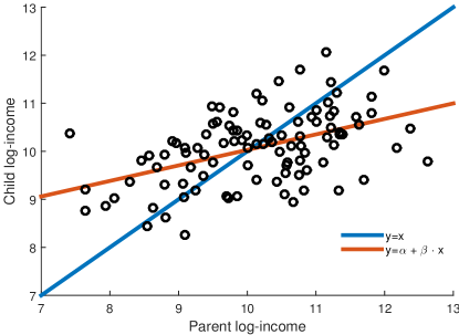
Figure 1: An illustration of the absolute and relative mobility measures. The black circles are a randomly chosen sample of 100 parent-child log-income pairs. The sample was created assuming a bivariate normal distribution and the parameters used were $\mu_{p}=10.1$, $\sigma_{p}=0.78$ (for the parents marginal distribution) and $\mu_{c}=10.25$, $\sigma_{c}=1.15$ (for the children marginal distribution) with correlation of $\rho=0.57$. The resulting $\alpha$ and $\beta$ were $1.8$ and $0.84$, respectively.

Since income distributions are known to be well approximated by the log-normal distribution pinkovskiy2009parametric , a simple plausible model for the joint distribution of parent and child log-incomes is the bivariate normal distribution. Under this assumption, the marginal income distributions of both parents and children are log-normal and the correlation between their log-incomes is defined by a single parameter $\rho$. The marginal log-income distribution of the parents (children) follows $\mathcal{N}\left(\mu_{p},\sigma_{p}^{2}\right)$ ($\mathcal{N}\left(\mu_{c},\sigma_{c}^{2}\right)$), hence the joint distribution is fully characterized by 5 parameters: $\mu_{p}$, $\sigma_{p}$, $\mu_{c}$, $\sigma_{c}$ and $\rho$.

Assuming the bivariate normal approximation for the joint distribution enables theoretically studying its properties. In particular Both measures of mobility, $A$ and $1-\beta$, can be derived directly from the model and, notably, can both be expressed analytically as functions of the other. We first derive the IGE in terms of the distribution parameters:

Proposition 1

For a bivariate normal distribution with parameters $\mu_{p}$, $\sigma_{p}$ (for the parents marginal distribution) and $\mu_{c}$, $\sigma_{c}$ (for the children marginal distribution) assuming correlation $\rho$, the IGE is

$$1-\beta=1-\frac{\sigma_{c}}{\sigma_{p}}\rho\,.$$ (.4)

Proof. First, by definition, the correlation $\rho$, between $X_{p}$ and $X_{c}$ equals to their covariance, divided by $\sigma_{p}\sigma_{c}$

$$\rho=\frac{\text{Cov}\left[X_{p},X_{c}\right]}{\sigma_{p}\sigma_{c}}\,.$$ (.5)

$\beta$ can be directly calculated as follows, by the linear regression slope definition:

$$\beta=\frac{\sum_{i=1}^{N}{\left(X_{p}^{i}-\bar{X}_{p}\right)\left(X_{c}^{i}-\bar{X}_{c}\right)}}{\sum_{i=1}^{N}{\left(X_{p}^{i}-\bar{X}_{p}\right)}}\,,$$ (.6)

where $\bar{X}_{p}$ and $\bar{X}_{c}$ are the average parents and children log-incomes, respectively.

It follows that

$$\beta=\frac{\text{Cov}\left[X_{p},X_{c}\right]}{\sigma_{p}^{2}}\,.$$ (.7)

We immediately obtain

$$\beta=\frac{\sigma_{c}}{\sigma_{p}}\rho$$ (.8)

and therefore

$$1-\beta=1-\frac{\sigma_{c}}{\sigma_{p}}\rho$$ (.9)

 

Following Prop. 1 it is also possible to derive the rate of absolute mobility as a function of the distribution parameters and the IGE:

Proposition 2

For a bivariate normal distribution with parameters $\mu_{p}$, $\sigma_{p}$ (for the parents marginal distribution), $\mu_{c}$, $\sigma_{c}$ (for the children marginal distribution) and $\rho=\sigma_{p}\beta/\sigma_{c}$ (where $\beta$ is the IGE), the rate of absolute mobility is

$$A=\Phi\left(\frac{\mu_{c}-\mu_{p}}{\sqrt{\sigma_{p}^{2}\left(1-2\beta\right)+\sigma_{c}^{2}}}\right)\,,$$ (.10)

where $\Phi$ is the cumulative distribution function of the standard normal distribution.

Proof. We start by defining a new random variable $Z=X_{c}-X_{p}$. It follows that calculating $A$ is equivalent to calculating the probability $P\left(Z>0\right)$.

Subtracting two dependent normal distributions yields that $Z\sim\mathcal{N}\left(\mu_{c}-\mu_{p},\sigma_{p}^{2}+\sigma_{c}^{2}-2\text{Cov}\left[X_{p},X_{c}\right]\right)$, so according to Prop. 1

$$Z\sim\mathcal{N}\left(\mu_{c}-\mu_{p},\sigma_{p}^{2}\left(1-2\beta\right)+\sigma_{c}^{2}\right)\,.$$ (.11)

If follows that

$$\frac{Z-\left(\mu_{c}-\mu_{p}\right)}{\sqrt{\sigma_{p}^{2}\left(1-2\beta\right)+\sigma_{c}^{2}}}\sim\mathcal{N}\left(0,1\right)\,,$$ (.12)

so we can now write

$$\begin{split}&P\left(Z>0\right)=\\ &P\left(\frac{Z-(\mu_{c}-\mu_{p})}{\sqrt{\sigma_{p}^{2}\left(1-2\beta\right)+\sigma_{c}^{2}}}>-\frac{\mu_{c}-\mu_{p}}{\sqrt{\sigma_{p}^{2}\left(1-2\beta\right)+\sigma_{c}^{2}}}\right)=\\ &\Phi\left(\frac{\mu_{c}-\mu_{p}}{\sqrt{\sigma_{p}^{2}\left(1-2\beta\right)+\sigma_{c}^{2}}}\right)\,,\end{split}$$ (.13)

where $\Phi$ is the cumulative distribution function of the standard normal distribution.

 

Proposition 2 shows that the rate of absolute mobility can be explicitly described as a function of the relative mobility.

References

- [1] Daniel Aaronson and Bhashkar Mazumder. Intergenerational economic mobility in the united states, 1940 to 2000. Journal of Human Resources, 43(1):139–172, 2008.
- [2] Yonatan Berman. Understanding the mechanical relationship between inequality and intergenerational mobility. SSRN, 2016. http://ssrn.com/abstract=2796563.
- [3] Raj Chetty, David Grusky, Maximilian Hell, Nathaniel Hendren, Robert Manduca, and Jimmy Narang. The fading american dream: Trends in absolute income mobility since 1940. Science, 356(6336):398–406, 2017.
- [4] Raj Chetty, Nathaniel Hendren, Patrick Kline, and Emmanuel Saez. Where is the land of opportunity? the geography of intergenerational mobility in the united states. The Quarterly Journal of Economics, 129(4):1553–1623, 2014.
- [5] Raj Chetty, Nathaniel Hendren, Patrick Kline, Emmanuel Saez, and Nicholas Turner. Is the united states still a land of opportunity? recent trends in intergenerational mobility. The American Economic Review, 104(5):141–147, 2014.
- [6] Miles Corak. Chasing the same dream, climbing different ladders: Economic mobility in the united states and canada. 2009. Economic Mobility Project, Pew Charitable Trusts Paper.
- [7] Miles Corak. Income inequality, equality of opportunity, and intergenerational mobility. The Journal of Economic Perspectives, 27(3):79–102, 2013.
- [8] Robert M. Hauser. What do we know so far about multigenerational mobility? Technical Report 98-12, UW-Madison Center for Demography and Ecology, 2010.
- [9] Chul-In Lee and Gary Solon. Trends in intergenerational income mobility. The Review of Economics and Statistics, 91(4):766–772, 2009.
- [10] Bhashkar Mazumder. Fortunate sons: New estimates of intergenerational mobility in the united states using social security earnings data. Review of Economics and Statistics, 87(2):235–255, 2005.
- [11] Casey B. Mulligan. Parental priorities and economic inequality. University of Chicago Press, 1997.
- [12] Maxim Pinkovskiy and Xavier Sala-i-Martin. Parametric estimations of the world distribution of income. 2009. Working Paper 15433, NBER.
- [13] John E. Roemer. Equality of Opportunity. Harvard University Press, Cambridge, MA, 2000.