Attached flow structure and streamwise energy spectra in a turbulent boundary layer:

Abstract

On the basis of (i) Particle Image Velocimetry data of a Turbulent Boundary Layer with large field of view and good spatial resolution and (ii) a mathematical relation between the energy spectrum and specifically modeled flow structures, we show that the scalings of the streamwise energy spectrum $E_{11}(k_{x})$ in a wavenumber range directly affected by the wall are determined by wall-attached eddies but are not given by the Townsend-Perry attached eddy model’s prediction of these spectra, at least at the Reynolds numbers $Re_{\tau}$ considered here which are between $10^{3}$ and $10^{4}$. Instead, we find $E_{11}(k_{x})\sim k_{x}^{-1-p}$ where $p$ varies smoothly with distance to the wall from negative values in the buffer layer to positive values in the inertial layer. The exponent $p$ characterises the turbulence levels inside wall-attached streaky structures conditional on the length of these structures.

I Introduction:

In the past forty years, the turbulence spectrum of velocity fluctuations in wall turbulence has received considerable attention as it gives valuable insight into the behaviour of wall-bounded flows by indicating the distribution of energy across scales. Spectral scaling laws built on ideas initiated by Townsend [townsend1976structure, ] , in particular the attached eddy hypothesis, have seen consistent development over the years (see Refs. Perry & Chong [perry1982mechanism, ], Perry et al. [perry1986theoretical, ], Perry & Li [perry1990experimental, ], Marusic et al. [marusic1997similarity, ] and Marusic & Kunkel [marusic2003streamwise, ]). Perry & Abell [perry1977asymptotic, ] and Perry et al. [perry1986theoretical, ] showed how Townsend’s attached eddy hypothesis implies that the energy spectrum $E_{11}(k_{x})$ of the turbulent streamwise fluctuating velocity at a distance $y$ from the wall scales as $E_{11}(k_{x})\sim U_{\tau}^{2}k_{x}^{-1}$ in the range $1/\delta\ll k_{x}\ll 1/y$ where $U_{\tau}$ is the friction velocity and $\delta$ is the boundary layer thickness. Nickels et al. [nickels2005evidence, ] stressed the use of overlap arguments to deduce the -1 power law behaviour. That is, a $k_{x}^{-1}$ region in the spectra would exist where the inner scaling (based on $y$ and $U_{\tau}$) and outer scaling (based on $\delta$ and $U_{\tau}$) are simultaneously valid over the same wavenumber range. Nickels et al. [nickels2007some, ] stated that it is necessary to take measurements surprisingly close to the wall to observe a $k_{x}^{-1}$ behaviour and thought this was the reason why Morrison et al. [morrison2004scaling, ] and McKeon & Morrison [mckeon2007asymptotic, ] did not observe any $-1$ region in their spectra as their measurements were not close enough to the wall. However, recent experiments by Vallikivi et al. [vallikivi2015spectral, ] do not show an overlap region and these authors infer that the $k_{x}^{-1}$ region cannot be expected even at very high Reynolds numbers.

The present work looks at the basis for the $k_{x}^{-1}$ range in flat plate turbulent boundary layers from a new perspective. Using Particle Image Velocimetry (PIV) and a simple model which can in principle be applied to various wall-bounded turbulent flows, we show how, in the turbulent boundary layer, a power-law spectral range exists but is not a Townsend-Perry $k_{x}^{-1}$ range and how it can be accounted for by taking only streamwise lengths and intensities of wall-attached structures into account.

This paper is organized as follows. In sections II and III we provide a model for the streamwise energy spectrum. The experimental set-up of the flat plate boundary layer is presented in section IV. Our data set is validated in V.1 and the method for educing the wall-attached flow structures relevant to our model is described in section V.2. The main results of the paper are in V.3 and V.4 followed by a discussion in V.5. We conclude in section VI.

II A simple model for the spectral signature of the Townsend-Perry attached eddy range of wavenumbers

As already mentioned in the introduction, Perry & Abell [perry1977asymptotic, ], Perry & Chong [perry1982mechanism, ] and Perry et al. [perry1986theoretical, ] showed how Townsend’s attached eddy hypothesis implies $E_{11}(k_{x})\sim U_{\tau}^{2}k_{x}^{-1}$ in the range $1/\delta\ll k_{x}\ll 1/y$. Perry et al. [perry1986theoretical, ] also developed a flow structure model for this spectral range in terms of specific attached eddies of varying sizes randomly distributed in space and with a number density that is inversely proportional to size. In this paper we attempt to distill such a type of model to its bare essentials. These bare essentials are that flow structures are primarily objects with clear spatial boundaries. In section V we model these boundaries with on-off functions in the expectation that the spectral signature in the attached eddy wavenumber range is dominated by these sharp gradient, effectively on-off, behaviours. The concomitant expectation is that the additional superimposed velocity fluctuations fill the content of a predominantly higher frequency spectral range. In this section we show that the streamwise energy spectrum’s $k_{x}^{-1}$ spectral range can be captured by simple on-off representations of elongated streaky structures of varying sizes as long as their number density has a space-filling power law dependence on size.

We therefore assume that the attached eddies responsible for the $k_{x}^{-1}$ spectral range have a long streaky structure footprint on the 1D streamwise fluctuating velocity signals at a distance $y$ from the wall. We also assume that these streaky structures can be modeled as simple on-off functions and that it is sufficient to represent the streamwise velocity fluctuations $u(x)$ at a given height $y$ from the wall as follows

$$u(x)=\sum_{n,m}a_{nm}\Pi(\xi)$$ (1)

where $\Pi(\xi)=1$ if $-1<\xi<1$ with $\xi={x-x_{nm}\over\lambda_{n}}$ and $\Pi(\xi)=0$ otherwise. The on-off function $\Pi(\xi)$ is our cartoon model of a streaky structure. Streaky structures of length $\lambda_{n}$ are centred at random positions $x_{nm}$ and their intensity is given by the coefficients $a_{nm}$. For each subscript $n$, the subscript $m$ counts the spatial positions where cartoon structures of size $\lambda_{n}$ can be centred in a given realisation. The sum in (1) is over all structures lengths $\lambda_{n}$ and all their positions $x_{nm}$.

The energy spectrum of $u(x)$ is $E_{11}(k_{x})={(2\pi)^{2}\over L_{x}}\overline{|\hat{u}(k_{x})|^{2}}$ where $L_{x}$ is the length of the record, $\hat{u}(k_{x})$ is the Fourier transform of $u(x)$, and the overbar signifies an average over realisations. The Fourier transform of $\Pi({x-x_{nm}\over\lambda_{n}})$ being $\hat{\Pi}(k_{x},\lambda_{n},x_{nm})=2ik_{x}^{-1}e^{ik_{x}x_{nm}}\sin(k_{x}\lambda_{n})$, it follows that

$$\hat{u}(k_{x})=2ik_{x}^{-1}\sum_{nm}a_{nm}e^{ik_{x}x_{nm}}\sin(k_{x}\lambda_{n})$$ (2)

which implies that the energy spectrum is given by

$$E_{11}(k_{x})=4{(2\pi)^{2}\over L_{x}}k_{x}^{-2}\overline{\sum_{nm}a_{nm}e^{ik_{x}x_{nm}}\sin(k_{x}\lambda_{n})\sum_{pq}a_{pq}e^{-ik_{x}x_{pq}}\sin(k_{x}\lambda_{p})}.$$ (3)

We introduce two assumptions which were also used by Perry et al. [perry1986theoretical, ] in their more intricate model. The first assumption is that the positions and amplitudes of our cartoon stuctures are uncorrelated and that different positions are not correlated to each other either, i.e. $\overline{e^{ik_{x}x_{nm}}e^{ik_{x}x_{pq}}}=\delta_{pn}\delta_{qm}$. As a result, the expression for the energy spectrum simplifies as follows:

$$E_{11}(k_{x})=4{(2\pi)^{2}\over L_{x}}k_{x}^{-2}\sum_{nm}\overline{(a_{nm})^{2}}\sin^{2}(k_{x}\lambda_{n}).$$ (4)

Let us say that there is an average number $N_{n}$ of cartoon stuctures of size $\lambda_{n}$ centred within an integral scale along the $x$-axis. The expression for $E_{11}(k_{x})$ simplifies even further:

$$E_{11}(k_{x})=4{(2\pi)^{2}\over L_{x}}k_{x}^{-2}\sum_{n}\overline{a_{n}^{2}}N_{n}\sin^{2}(k_{x}\lambda_{n})$$ (5)

where $\overline{a_{n}^{2}}\equiv\overline{(a_{nm})^{2}}$ is the same irrespective of position $x_{nm}$.

We now consider a continuum of different structure sizes $\lambda$ rather than discrete length-scales $\lambda_{n}$ and the previous expression for $E_{11}(k_{x})$ must therefore be replaced by

$$E_{11}(k_{x})=4{(2\pi)^{2}\over L_{x}}k_{x}^{-2}\int d\lambda\overline{a^{2}}(\lambda)N(\lambda)\sin^{2}(k_{x}\lambda)$$ (6)

in terms of easily understandable notation. At this point we introduce a generalised form of the second assumption which was also used by Perry et al. [perry1986theoretical, ]: we assume a power-law form for $N(\lambda)$ in the range $\lambda_{i}<\lambda<\lambda_{o}$ where $\lambda_{i}\sim y$ and $\lambda_{o}\sim\delta$, and $N(\lambda)=0$ outside this range for simplicity. This power law form is $N(\lambda)=(-N_{M}+N_{o}(\lambda/\delta)^{-1-D})$ where $N_{M}$ and $N_{o}$ are positive dimensionless numbers which increase propotionally to $L_{x}$ so as to keep number densities constant. The number $N_{M}$ is introduced to allow for the possibility of an upper bound on streaky structure size given by $N(\lambda_{o})=0$, i.e. $N_{M}=N_{o}(\lambda_{o}/\delta)^{-1-D}$ which should be small given that LSM and VLSM streaky structures have been observed with lengths greater than $\delta$ [see Smits et al. smits2011high, ].

Vassilicos & Hunt [vassilicos1991fractal, ] proved that, if $0\leq D\leq 1$, then the set of points defining the edges of the on-off functions $\Pi(\xi)$ is fractal and $D$ is effectively the fractal dimension of this set of points. The case where this fractal dimension is $D=1$ is the case where these points are space-filling. The population density assumption of Perry et al. [perry1986theoretical, ] corresponds to $D=1$ which is also the choice we make in this work. We now show that this choice can lead to $E_{11}(k_{x})\sim k_{x}^{-1}$ in the range $1/\lambda_{o}\ll k_{x}\ll 1/\lambda_{i}$.

We calculate the energy spectrum by carrying out the integral in (6). This requires a model for $\overline{a^{2}}(\lambda)$ which, in this section, we chose to be as simple as possible and therefore independent of $\lambda$ in the relevant range, i.e. $\overline{a^{2}}(\lambda)=A^{2}/\delta$ for $\lambda_{i}<\lambda<\lambda_{o}$ where $A^{2}$ is a constant. Using our models for $N(\lambda)$ and $\overline{a^{2}}(\lambda)$ and the change of variables $\lambda k_{x}=l$, (6) becomes

$$E_{11}(k_{x})=A^{2}\delta(C_{o}(k_{x}\delta)^{-2+D}-C_{M}(k_{x}\delta)^{-2})$$ (7)

where

$$C_{o}=4(2\pi)^{2}N_{o}{\delta\over L_{x}}\int_{\lambda_{i}k_{x}}^{\lambda_{o}k_{x}}dl\sin^{2}(l)l^{-1-D}$$

and

$$C_{M}=4(2\pi)^{2}N_{M}{\delta\over L_{x}}(k_{x}\delta)^{-1}\int_{\lambda_{i}k_{x}}^{\lambda_{o}k_{x}}dl\sin^{2}(l)$$

which is bounded from above by ${N_{M}\over L_{x}}{\lambda_{o}-\lambda_{i}\over\delta}$. In the attached eddy range $1/\lambda_{o}\ll k_{x}\ll 1/\lambda_{i}$, $C_{o}\approx 4(2\pi)^{2}{N_{o}\over L_{x}}\int_{0}^{\infty}dl\sin^{2}(l)l^{-1-D}$ which means that $C_{o}$ is approximately independent of $k_{x}$ in this range.

Substituting the value $D=1$ in equation (7), we get $E_{11}(k_{x})=A^{2}(C_{o}k_{x}^{-1}-C_{M}\delta^{-1}k_{x}^{-2})$ which is well approximated by

$$E_{11}(k_{x})\approx C_{o}A^{2}k_{x}^{-1}$$ (8)

for wavenumbers $k_{x}\delta\gg C_{M}/C_{o}$ (i.e. $C_{o}k_{x}^{-1}\gg C_{m}\delta^{-1}k_{x}^{-2}$). Note that $C_{M}/C_{o}$ is much smaller than 1 because $N_{M}$ is much smaller than $N_{o}$ and that (8) is valid in the range $1/\lambda_{o}\ll k_{x}\ll 1/\lambda_{i}$ where $\lambda_{o}$ scales with but is much larger than $\delta$. For a good correspondence with the scalings of the Townsend-Perry attached eddy model one needs to take $\lambda_{i}\sim y$ and $A^{2}\sim U_{\tau}^{2}$.

III A straightforward generalisation

It is worth generalising the previous section’s model by assuming that $\overline{a^{2}}(\lambda)$ is not constant but varies with $\lambda$ in the range $\lambda_{i}<\lambda<\lambda_{o}$, for example as $\overline{a^{2}}(\lambda)=(A^{2}/\delta)(\lambda/\delta)^{p}$ where $p$ is a real number with bounds which we determine below. The arguments of the previous section can be reproduced till equation (6) which now becomes

$$E_{11}(k_{x}) = A^{2}\delta[c_{o}(k_{x}\delta)^{-2+D-p}-c_{M}(k_{x}\delta)^{-2}]$$ (9)

where

$$c_{o}=4(2\pi)^{2}N_{o}{\delta\over L_{x}}\int_{\lambda_{i}k_{x}}^{\lambda_{o}k_{x}}dl\sin^{2}(l)l^{-1-D+p}$$

and

$$c_{M}=4(2\pi)^{2}N_{M}{\delta\over L_{x}}(k_{x}\delta)^{-1-p}\int_{\lambda_{i}k_{x}}^{\lambda_{o}k_{x}}dl\;l^{+p}\sin^{2}(l)$$

which is bounded from above by ${N_{m}\over(1+p)L_{x}}[({\lambda_{o}\over\delta})^{1+p}-({\lambda_{i}\over\delta})^{1+p}]$. In the attached eddy range $1/\lambda_{o}\ll k_{x}\ll 1/\lambda_{i}$, $c_{o}\approx 4(2\pi)^{2}{N_{o}\over L_{x}}\int_{0}^{\infty}dl\sin^{2}(l)l^{-1-D+p}$ which means that $c_{o}$ is approximately independent of $k_{x}$ in this range if $0<D-p<2$.

Substituting the value $D=1$ in (9), we obtain the following leading order approximation in the parameter range $-1<p<1$:

$$E_{11}(k_{x})\approx c_{0}A^{2}\delta(k_{x}\delta)^{q}$$ (10)

where

$$p+q=-1$$ (11)

for wavenumbers $k_{x}\delta\gg(c_{M}/c_{o})^{{1\over 1-p}}$. Note that $c_{M}/c_{o}$ is much smaller than 1 if $p$ is not too close to $1$ because $N_{M}$ is much smaller than $N_{o}$.

The spectral shape (10) is potentially significantly different from what the classical Townsend-Perry attached eddy model predicts. We emphasize that in this and the previous sections we have developed a simple model based on on-off functions representing long streaky structures which returns a wavenumber dependency of $E_{11}(k_{x})$ which is either identical to the Townsend-Perry spectral shape if $p=0$, or different but in some ways comparable if $p\not=0$. In the remainder of this paper we present experimental evidence in support of $D=1$ and (10)-(11) rather than (8), with $p$ as function of $y^{+}$.

IV Experimental set-up

An experiment was performed in the boundary layer wind tunnel at the Lille Mechanics Laboratory (LML) having a test section $2$m wide, 1m high and $20.6$m long. The tests were conducted at two free stream velocities of $3$m/s and $10$m/s corresponding to Reynolds numbers $Re_{\theta}=8100$ ($Re_{\tau}=2700$) and $Re_{\theta}=20600$ ($Re_{\tau}=7200$) respectively. To capture the large streamwise wall-normal field, four $12$ bits Hamamatsu cameras having a resolution of $2048$x$2048$ pixels were installed in series to observe a region between $19.26$m and $20.42$m from inlet which is $1.16$m long ($\approx 3.36\delta$ and $3.85\delta$, for $Re_{\theta}=8100$ and $20600$ respectively) and 0.3m high ($\approx 0.86\delta$ and $1\delta)$ for $Re_{\theta}=8100$ and $20600$ respectively). Nikon lenses of 50mm focal length were set on the cameras and the magnification obtained was 0.05. The Software HIRIS was used to acquire the images of the four cameras simultaneously. A total of $22500$ and $29500$ samples were recorded at the highest and lowest Reynolds numbers respectively. The flow was seeded with $1\mu m$ Poly-Ethylene glycol and illuminated by a double pulsed NdYAG laser at $400$mJ/pulse. The modified version by LML of MatPIV toolbox, was used under Matlab to process the acquired images from the 2D2C PIV. A multipass software was used with a final pass of 28x28 pixels (with a mean overlap of $65\%$) corresponding to 4mm x 4mm i.e. 33x33 wall units for $Re_{\theta}=8100$ and 100x100 wall units for $Re_{\theta}=20600$. Image deformation was applied at the final pass. The final grid had $766$ points along the wall and 199 points in the wall-normal direction with a grid spacing of $1.5$mm corresponding to 11 wall units and $35$ wall units for the test cases at $Re_{\theta}=8100$ and $Re_{\theta}=20600$ respectively.

V Results and discussion

V.1 Validation of experimental data

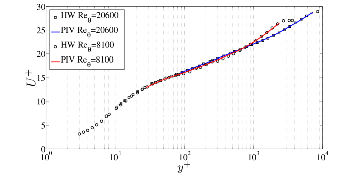
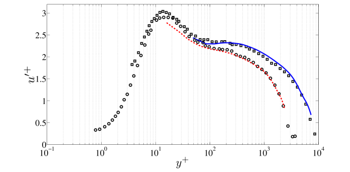
Figure 1: Mean streamwise velocity profiles (top) and rms streamwise fluctuating velocity profiles (bottom) at $Re_{\theta}=8100$ ($U_{\infty}=3m/s$) and $Re_{\theta}=20600$ ($U_{\infty}=10m/s$) obtained with PIV and compared with the hot wire anemometry results of Carlier & Stanislas [carlier2005experimental, ].

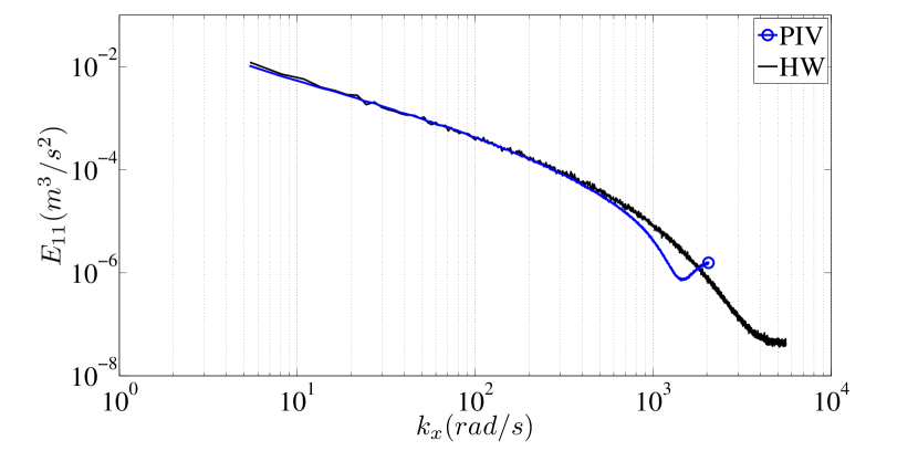
Figure 2: Comparison of the streamwise energy spectra obtained from PIV and hot-wire anemometry at $y^{+}=200$ for $Re_{\theta}=20600$. $E_{11}(k_{x})$ is in $m^{3}/s^{2}$ and $k_{x}$ is in $rad/m$. The hot-wire anemometry was made by Carlier & Stanislas [carlier2005experimental, ] at $19.6$m from wind tunnel inlet in the same wind tunnel.

Figure 1 shows profiles of the mean streamwise velocity $U$ and the rms streamwise fluctuating velocity $u^{\prime}$ obtained from PIV at $Re_{\theta}=8100$ and $Re_{\theta}=20600$ and compared with the hot-wire anemometry results of Carlier & Stanislas [carlier2005experimental, ]. The mean velocity profiles are in good agreement with the hot-wire data and are well resolved from $y^{+}\approx 30$ and $y^{+}\approx 90$ upwards for $Re_{\theta}=8100$ and $20600$ respectively. Comparisons of the profiles of $u^{\prime+}$ ($u^{\prime}$ scaled with inner variables) show a fairly good match with the hot-wire data. A plateau of $u^{\prime+}$ is present in the range $100<y^{+}<300$ for our higher Reynolds number case. Close to the wall, the $u^{\prime+}$ values obtained from our PIV are slightly underestimated, in particular for $Re_{\theta}=20600$, demonstrating some filtering of the PIV at this resolution (Foucaut et al. [foucaut2004piv, ]). To compute from PIV the energy spectra used in this paper, we used the method of Foucaut et al. [foucaut2004piv, ]. As seen in figure 2 for the particular case of wall distance $y^{+}=200$ at $Re_{\theta}=20600$, the agreement between the spatial spectrum from the PIV and the temporal spectrum from the hot-wire anemometry of Carlier & Stanislas [carlier2005experimental, ] is good up to wavenumbers $k_{x}\approx 500$ corresponding to length-scales of $2$mm.

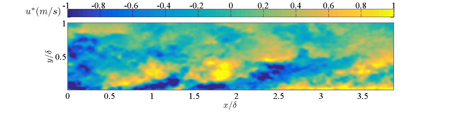
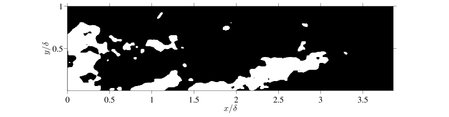
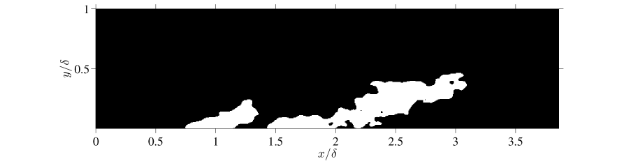
Figure 3: Wall-attached elongated streaky structure eduction method applied on a sample instantaneous streamwise velocity field at $Re_{\theta}=20600$. From top: (a) Raw instantaneous streamwise fluctuating velocity component field (b) The same field after application of a Gaussian filter (c) Binary image obtained after thresholding negative streamwise fluctuating momentum regions. (d) Final image obtained after cleaning as described in subsection V.2.

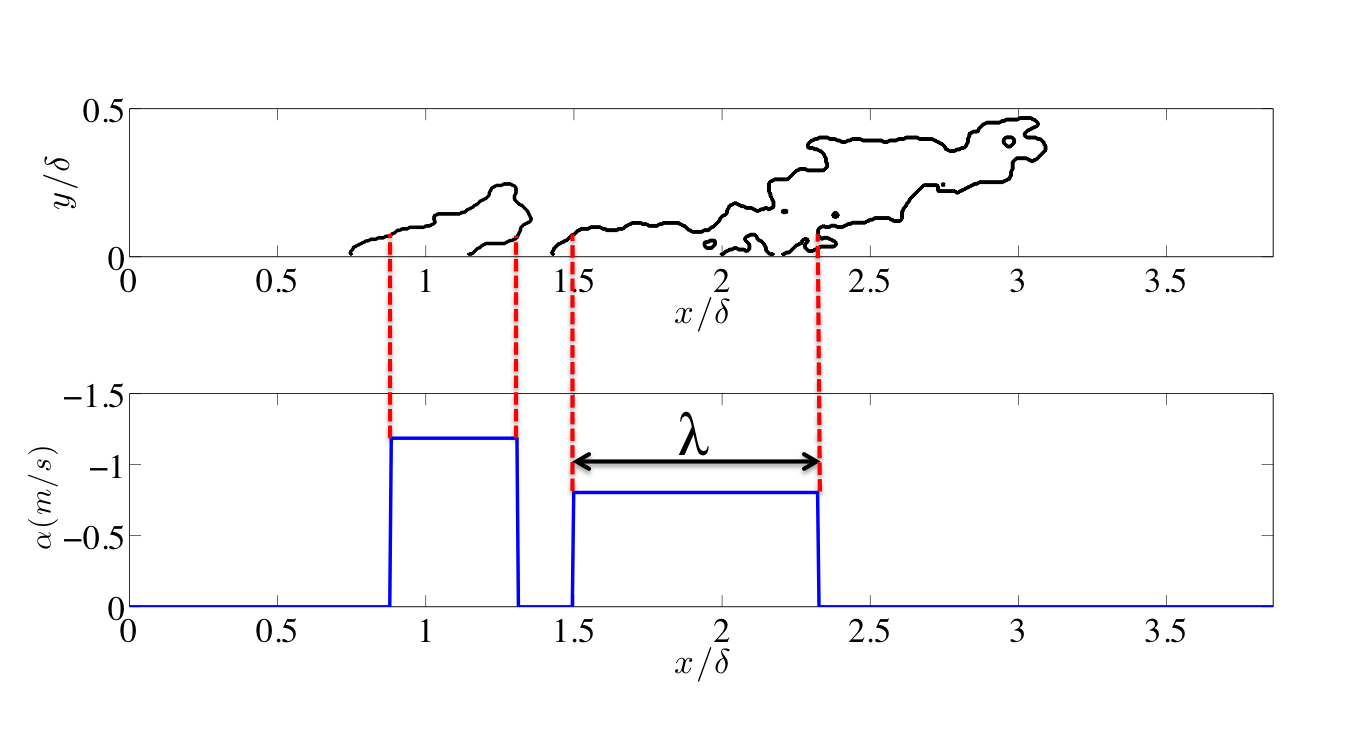
Figure 4: Figure 3(d) reproduced in the top plot, with, in the bottom plot, the average streamwise fluctuating velocity $\alpha$ and the streamwise length $\lambda$ of the detected wall-attached structures at $y/\delta=0.03$.

V.2 Structure detection

In sections II and III we developed a spectral model of the streamwise turbulence fluctuating velocity based on the concept of elongated streaky structures which are part of attached eddies and can be modeled as simple on-off functions. In this and the next subsections we use our PIV data to test this concept and assess its potential as an hypothesis for understanding near-wall streamwise energy spectra.

Figure 3(a) shows a sample field of instantaneous streamwise fluctuating velocity components $u$. The existence of well-defined elongated and tilted wall-attached regions of relatively high (positive or negative) $u$ values is clear. It is these regions that we need to target in relation to the elongated streaky structures of our model.

The raw instantaneous streamwise velocity fields are affected by noise so that single structures in figure 3(a) appear split in many little parts. To smooth out these structures without modifying their shape and statistics we used a two-dimensional Gaussian filter. This filtering operation was found to be sufficient to capture and connect the structures while retaining their overall shape. The standard deviation of the Gaussian filter was three pixels which corresponds to approximately $0.015\delta$ for both Reynolds numbers, i.e. 105 wall units for $Re_{\theta}=20600$ and 33 wall units for $Re_{\theta}=8100$. The result of this operation on figure 3(a) leads to figure 3(b).

To educe on-off functions such as the ones required by our model we apply a threshold $u_{th}$ on the gaussian-filetered $u^{*}$ to obtain binary images which distinguish between $u^{*}<u_{th}$ and $u^{*}>u_{th}$. Effects of the threshold on the statistics of educed structures were investigated in the range $0.1u^{\prime}_{300^{+}}<|u_{th}|<u^{\prime}_{300^{+}}$ where $u^{\prime}_{300^{+}}$ is $u^{\prime}$ at $y^{+}=300$.

A threshold $u_{th}$ equal to $-0.4u^{\prime}_{300^{+}}$ was finally chosen to detect low momentum structures in the present study as it corresponds to the value that leads to least threshold-dependency of our statistics for a negative $u_{th}$ (for example, $u_{th}$ equal to $-0.2u^{\prime}_{300^{+}}$ or $-0.6u^{\prime}_{300^{+}}$ return results with no significant difference, see Appendix A). This thresholding operation leads to figure 3(c) when applied to figure 3(b). The white structures in figure 3(c) correspond to $u^{*}<u_{th}$.

One more step is required before comparing with our model. White structures which cut through the vertical borders of the figure are discarded because their streamwise extent is unknown; and white structures which are not attached to the bottom wall (at $y=0$ but in fact as close to $y=0$ as allowed by our PIV data, i.e. $y^{+}=16$ and $y^{+}=48$ for the lower and the higher Reynolds number cases respectively) are also discarded because we are concerned with wall-attached structures. With this extra step, figure 3(c) gives rise to figure 3(d).

All the steps leading from raw fluctuating streamwise velocity fields to the binary fields which we use in our statistical analysis are depicted in figure 3. The current study’s effort is concentrated on wall-attached elongated structures of negative streamwise fluctuating velocity as in figure 3(d), but the analysis can be repeated equally well on structures of positive streamwise fluctuating velocity with results that are similar though slightly less sharp with regard to (10)-(11) (see Appendix A). The general behaviours of positive and negative fluctuating streamwise velocity structures are similar, the negative velocity structures being slightly longer in agreement with Dennis & Nickels [dennis2011b, ].

V.3 Lengths of wall-attached streamwise velocity structures

We now need to obtain statistics of wall-attached elongated streaky structures represented as on-off functions in our model and as binary structures in the final stages of our structure eduction method. We first label the connected components of the binary images using image processing tools. Then we compute the streamwise length $\lambda$ of each labelled structure at a distance $y$ from the wall, i.e. the difference between the smallest and the largest values of streamwise coordinate $x$ in this labelled structure at height $y$. Finally we compute the average value $\alpha$ of the streamwise fluctuating velocity component $u$ inside this labelled structure at height $y$. Thus we obtain a pair $(\lambda,\alpha)$ for each labelled structure at each height $y$ considered. This procedure is illustrated in figure 4 where the streamwise extent $\lambda$ and the corresponding amplitude $\alpha$ of two labelled structures at wall distance $y/\delta=0.03$ is shown. A total of 14493 and 19576 wall-attached binary structures were detected at $Re_{\theta}=20600$ and $Re_{\theta}=8100$ respectively. (As mentioned in section IV, 22500 and 29500 samples were recorded at the highest and lowest of our two values of $Re_{\theta}$ respectively, and the ratios $14930/22500$ and $19576/29500$ are about the same.)

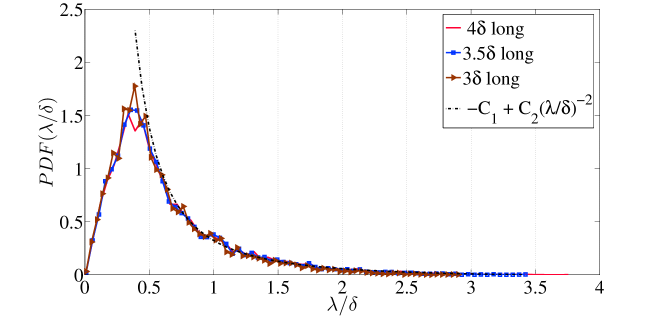
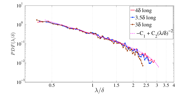
Figure 5: PDFs of streamwise lengths $\lambda$ (see figure 4) for varying domain lengths at wall distance $y^{+}=195$ for $Re_{\theta}=20600$. Lin-lin plot (top) and premultiplied log-log plot (bottom)

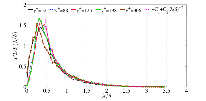
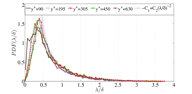
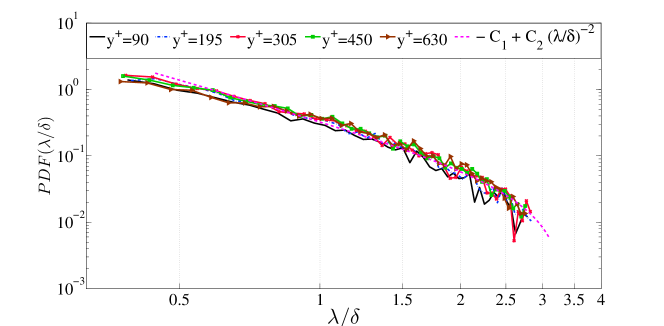
Figure 6: PDFs of streamwise lengths $\lambda$ of wall-attached structures (see figure 4) at selected wall distances for $Re_{\theta}=8100$ (top) and $Re_{\theta}=20600$ (middle). The fits shown in these top and middle plots are for $y^{+}=198$ at $Re_{\theta}=8100$ and $y^{+}=195$ at $Re_{\theta}=20600$. The bottom plot is a log-log reproduction of the middle plot’s data.

The model in sections II and III assumes that the number of wall-attached elongated streaky structures of size $\lambda$ has a decreasing power-law dependence on $\lambda$ in a certain range of $\lambda$ values. Following Perry et al. [perry1986theoretical, ], we expect the spatial distribution of such structures to be space-filling, which implies (see Vassilicos & Hunt [vassilicos1991fractal, ]) that the exponent of this power law should be -2. Figures 5 and 6 show the probability distribution function (PDF) of lengths $\lambda$ at various wall distances. The most probable length $\lambda$ lies between $0.3\delta$ and $0.5\delta$ and lengths $\lambda$ longer than 3.5$\delta$ occur very rarely.

We tested for finite size effects of the field of view by computing the PDF on smaller domains, namely 3.5$\delta$ and 3$\delta$ long in the streamwise direction but same in the wall normal direction. As shown in figure 5 there is no significant differences caused by the three fields of view except that the smallest field returns a slightly more noisy PDF. Indeed, a reduced field of view leads to a smaller number of detected wall-attached elongated binary structures and therefore to reduced statistical convergence.

Figures 5 and 6 show a power law dependence on $\lambda$ between about $0.5\delta$ and $2\delta$ with power law exponent -2, i.e. $D=1$, in all cases. Given the form of $N(\lambda)$ hypothesised in sections II and III, we fit the PDF of $\lambda/\delta$ with a functional form $-C_{1}+C_{2}(\lambda/\delta)^{-2}$ (where $C_{1}/N_{M}=C_{2}/N_{o}$). The fit is shown in figures 5 and 6 and is effectively the same for both Reynolds numbers and all values of $y^{+}$ in the mean flow’s approximate log region. The constants $C_{1}$ and $C_{2}$ are reported in table 1. They are indeed fairly constant over the range of wall distances and for both Reynolds numbers. Identical results are obtained for wall-attached structures with positive streamwise fluctuating velocity except that $C_{1}\approx 0.02$ for both Reynolds numbers and $C_{2}\approx 0.29$ for $Re_{\theta}=8100$ (see Table 3 in Appendix). It is worth noting that the lower bound of the range where the PDF of $\lambda/\delta$ is well approximated by $-C_{1}+C_{2}(\lambda/\delta)^{-2}$ seems to increase slightly with increasing $y^{+}$.

$Re_{\theta}$	20600					8100
$y^{+}$	90	195	305	450	630	52	88	125	198	306
$C_{1}$	0.03	0.03	0.03	0.03	0.03	0.04	0.04	0.04	0.03	0.03
$C_{2}$	0.32	0.35	0.35	0.37	0.37	0.32	0.35	0.35	0.35	0.33

Table 1: Values of the constants $C_{1}$ and $C_{2}$ in the form $-C_{1}+C_{2}(\lambda/\delta)^{-2}$ of the PDF of $\lambda/\delta$. In the $Re_{\theta}=20600$ case, the fit is over a range of $\lambda/\delta$ bounded from above by 3.8 and from below by 0.49 ($y^{+}=90$), 0.55 ($y^{+}=195$), 0.54 ($y^{+}=305$), 0.58 ($y^{+}=450$) and 0.78 ($y^{+}=630$). In the $Re_{\theta}=8100$ case, the fit is over a range of $\lambda/\delta$ bounded from above by 3.4 and from below by 0.54 ($y^{+}=52$), 0.53 ($y^{+}=88$), 0.53 ($y^{+}=125$), 0.56 ($y^{+}=198$) and 0.65 ($y^{+}=306$).

V.4 Energy spectra

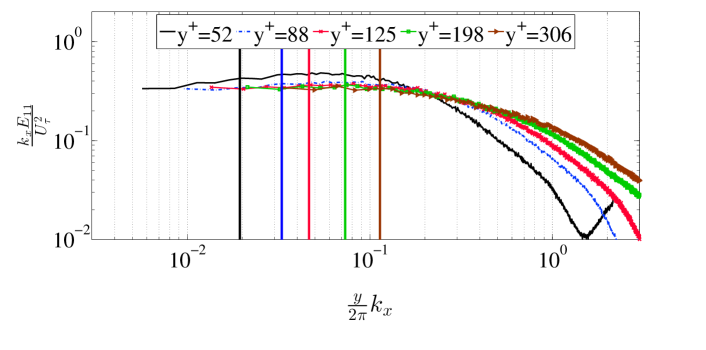
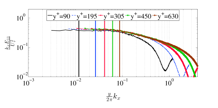
Figure 7: Log-log plots of pre-multiplied streamwise energy spectra at selected wall distances for $Re_{\theta}=8100$ above and $Re_{\theta}=20600$ below. Vertical lines show ${y\over 2\pi}k_{x}=(y/2\pi)(2\pi/\delta)=\frac{y}{\delta}$ (corresponding to $k_{x}=2\pi/\delta$) with the same color code as the legend of the figure.

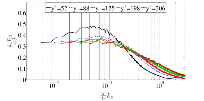
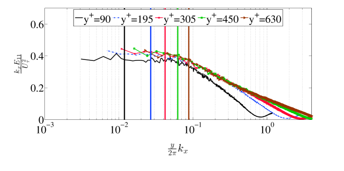
Figure 8: Same as figure 7 in lin-log plots.

Figure 7 shows log-log plots of premultiplied energy spectra of streamwise fluctuating velocities $u(x)$ which have been obtained from our PIV data at various normalised wall distances $y^{+}$ for both Reynolds numbers. These plots might suggest that $E_{11}(k_{x})\sim U_{\tau}^{2}k_{x}^{-1}$ in a range of wavenumbers $2\pi/(4\delta)\lesssim k_{x}\lesssim 0.63/y$ for $y^{+}$ larger than about 88 and smaller than the value of $y^{+}$ where this range of wavenumbers no longer exists. The apparent $k_{x}^{-1}$ wavenumber range is close to a decade long at $y^{+}=90$ for $Re_{\theta}=20600$ and shorter for higher wall normal distances and for the lower Reynolds number ($Re_{\theta}=8100$). One would be justified to conclude that this is indeed experimental support for the Townsend-Perry $k_{x}^{-1}$ spectrum if the only available theoretical glasses through which to look at these spectral plots were those of the Townsend-Perry attached eddy model. However the situation is subtler and, in effect, quite different.

A closer look at the spectra in the lin-log plot of figure 8 suggests the possibility for small corrections to this conclusion, particularly at the lower of the two $Re_{\theta}$ values, but the result (10)-(11) of our model in section III may pave the way for a significantly different interpretation. This model leads to $E_{11}(k_{x})\sim(k_{x}\delta)^{q}$ with $p+q=-1$ if $D=1$. Support for $D=1$ has been obtained and reported in the previous subsection in the range of lengths $\lambda$ between about $0.5\delta$ and $2\delta$. It is therefore worth taking a closer look at our energy spectra in the corresponding wavenumber range. For our data, this wavenumber range turns out, in fact, to be comparable to the wavenumber range $2\pi/(4\delta)\lesssim k_{x}\lesssim 0.63/y$ mentioned in the previous paragraph as a candidate for Townsend-Perry scaling. Specifically, $k_{x}/(2\pi)=2/\delta$ corresponds to $k_{x}y/(2\pi)=0.25$, $0.41$, $0.58$, $0.91$ and $1.41$ in increasing order of the $y^{+}$ values in figures 7 and 8 for $Re_{\theta}=8100$; and to $k_{x}y/(2\pi)=0.15$, $0.33$, $0.53$, $0.78$ and $1.1$ in increasing order of the $y^{+}$ values in figures 7 and 8 for $Re_{\theta}=20600$. The wavenumber range $0.5/\delta\leq k_{x}/(2\pi)\leq 2/\delta$ where the analysis in the remainder of our paper is carried out is therefore not radically different for our data from the wavenumber range $2\pi/(4\delta)<k_{x}<0.63/y$ where one would interpret our spectra to have a Townsend-Perry scaling for $y^{+}\geq 88$.

In figures 9 to 12 we plot $\overline{a^{2}}$ versus $\lambda/\delta$ where $\overline{a^{2}}$ is the average of $\alpha^{2}/\Delta\lambda$ conditional on the streamwise length of a labelled structure being between $\lambda$ and $\lambda+\Delta\lambda$ ($\alpha$ and $\lambda$ being obtained as explained in the first paragraph of subsection V.3). The upper values of $\lambda/\delta$ in these plots are all below about 2.3 because we do not have enough samples of educed structures beyond $\lambda/\delta\approx 2.3$ to obtain values of $\overline{a^{2}}$ which are statistically converged. The lower values of $\lambda/\delta$ in these plots are all close to $1/2$ because the range where the PDF of $\lambda/\delta$ has been found in the previous subsection to be well approximated by $-C_{1}+C_{2}(\lambda/\delta)^{-2}$ is bounded from below by about $1/2$ in all our $y^{+}$ and $Re_{\theta}$ cases. In figures 9 to 12 we also plot $E_{11}(k_{x})$ in the corresponding wavenumber range $0.25/\delta\leq k_{x}/(2\pi)\leq 2/\delta$ which, as discussed in the previous paragraph, may be close to the wavenumber range $2\pi/(4\delta)<k_{x}<0.63/y$ that one could interpret as a Townsend-Perry range. We do not have enough data and high enough Reynolds numbers to clearly distinguish between these two ranges in the present work.

As an aside for the moment, note that the large-scale motions (LSMs) and very large-scale motions (VLSMs), which have been found to exist in the logarithmic and lower wake regions of a turbulent boundary layer (see Kovasznay et al. [kovasznay1970large, ], Brown & Thomas [brown1977large, ], Hutchins & Marusic [hutchins2007evidence, ], Dennis & Nickels [dennis2011a, ] and Lee & Sung [lee2011very, ]) generally refer to elongated regions of streamwise velocity fluctuations having a streamwise extent from about $2\delta$ to $3\delta$ for LSMs and larger than $3\delta$ for VLSMs (see Kim & Adrian [kim1999very, ], Guala et al. [guala2006large, ] and Balakumar & Adrian [balakumar2007large, ]). The LSMs near the wall and the VLSMs have been interpreted as being responsible for the $k_{x}^{-1}$ scaling range of the turbulence spectrum (Smits et al. [smits2011high, ]). The range of scales we concentrate on, in figures 9 to 12, just about includes some LSMs at its upper range.

Returning now to figures 9 to 12, we have included best fits of power law curves in the plots of $\overline{a^{2}}$ versus $\lambda/\delta$ and of $E_{11}$ versus $k_{x}$. These best fits are indicated in the inserts of each plot and provide an estimation of the exponents $p$ and $q$ in $\overline{a^{2}}\sim(\lambda/\delta)^{p}$ and $E_{11}(k_{x})\sim k_{x}^{q}$. Figure 13 summarizes the information with plots of $p$, $q$ and $p+q$ as functions of $y^{+}$. It is perhaps remarkable that $p+q$ is very close to $-1$ (see figure 13) as predicted by (10)-(11) for all examined values of $y^{+}$ and for both Reynolds numbers $Re_{\theta}$. Whereas this subsection’s initial interpretation in terms of the Townsend attached eddy model is limited to $y^{+}$ larger or equal to $88$ (based on the log-log plots of figure 7), the lin-lin plots of figures 9 to 12 present a different and consistent picture which covers both Reynolds numbers and all our $y^{+}$ positions, including $y^{+}$ smaller than $88$. This picture is confirmed by Hot Wire Anemometry (HWA) data from a turbulent boundary layer in the same wind tunnel by Tutkun et al. [tutkun09, ] and from the recent Direct Numerical Simulations (DNS) of a turbulent channel flow at $Re_{\tau}=5200$ by Lee & Moser [leemoser15, ]. Indeed, these HWA and DNS data show the same variation of the spectral exponent $q$ with $y^{+}$ that we found from using (10)-(11) on our PIV data; see figure 14, and also figure 13(b) where we collected the values of $q$ from different data. The HWA data, in particular, provide a confirmation of our PIV results because they extend to a wider range at the lower end of wavenumbers (see figures 14(a) and also figure 13(b) where it is shown that the HWA’s extended wavenumber range returns effectively same values of $q$).

The much higher Reynolds number measurements of Vallikivi et al. [vallikivi2015spectral, ] did not find support for the Townsend-Perry $k_{x}^{-1}$ spectrum either. However, these authors did find some agreement with the $k_{x}^{-1}\log(8\pi/k_{x}y)$ spectrum model of del Álamo et al. [alamo04, ]. This approximate agreement was found in a range of wall-normal distances where we find positive values of $p$, i.e. in a region where the spectrum scales as $k_{x}^{-1}k_{x}^{-p}$ with values of $p$ above but close to $0$. It is quite difficult to distinguish between such a weak power law and $\log(8\pi/k_{x}y)$, so the two models qualitatively agree in this range of wall-normal distances. However, the model of del Álamo et al. [alamo04, ] cannot account for the scaling of the energy spectrum at closer distances to the wall where we find $p\leq 0$, whereas our model fits the data in this region too.

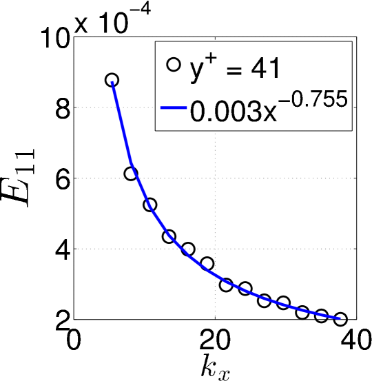
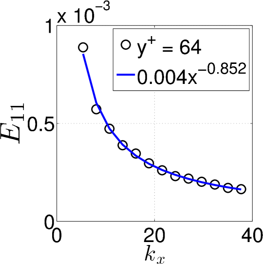
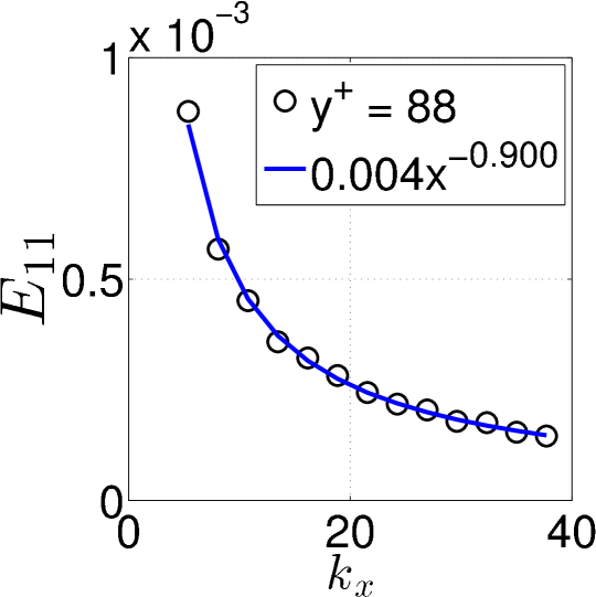
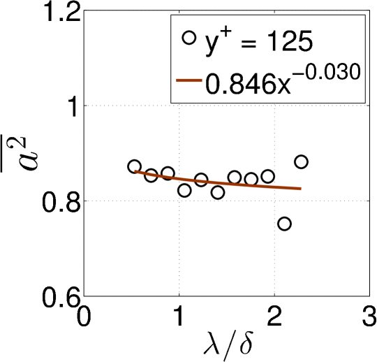
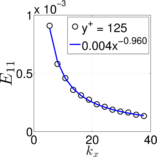
Figure 9: Lin-lin plots of $\overline{a^{2}}$ versus $\lambda/\delta$ (left) and streamwise energy spectra plotted at wall distances $y^{+}=$ 41, 64, 88 and 125 (from top to bottom) at $Re_{\theta}=8100$.

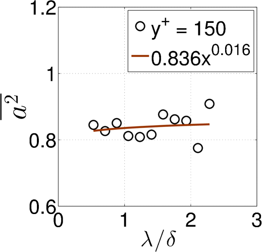
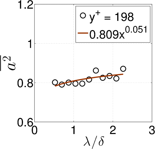
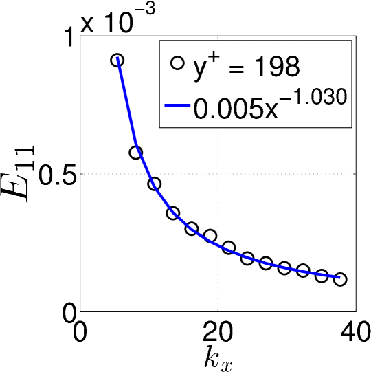
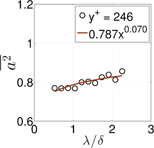
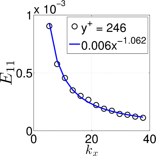
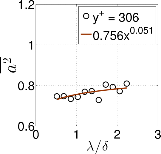
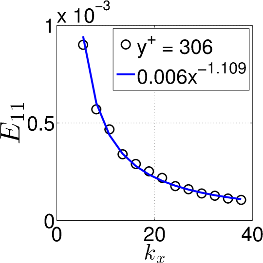
Figure 10: Lin-lin plots of $\overline{a^{2}}$ versus $\lambda/\delta$ (left) and streamwise energy spectra plotted at wall distances $y^{+}=$ 150, 198, 246 and 306 (from top to bottom) at $Re_{\theta}=8100$.

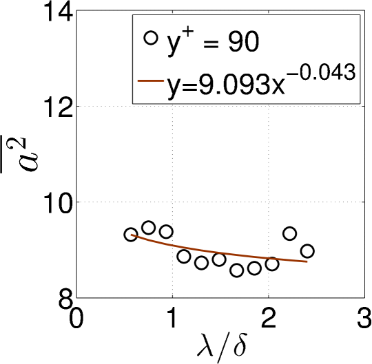
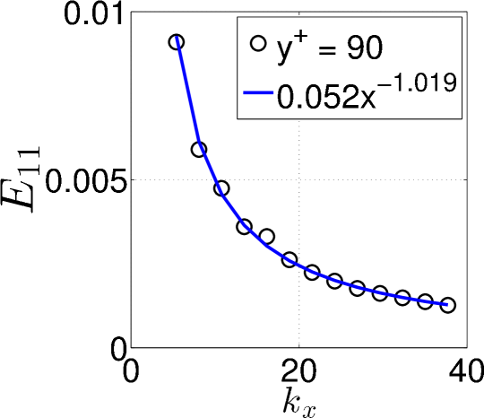
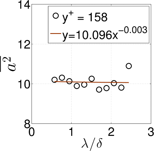
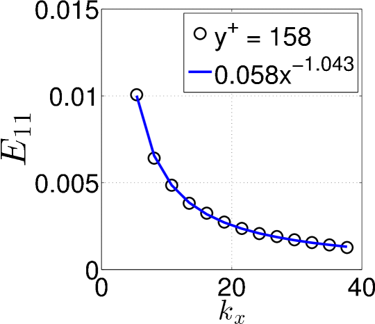
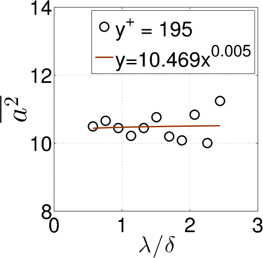
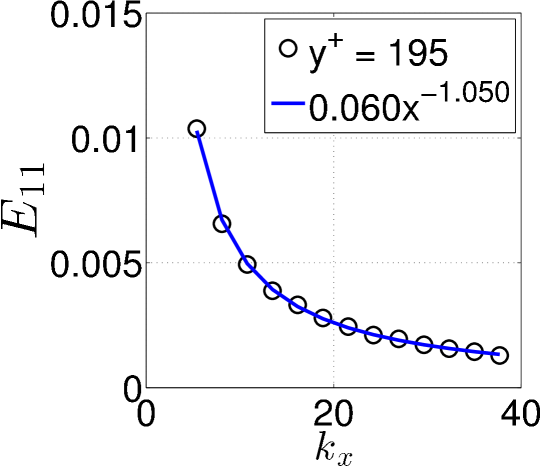
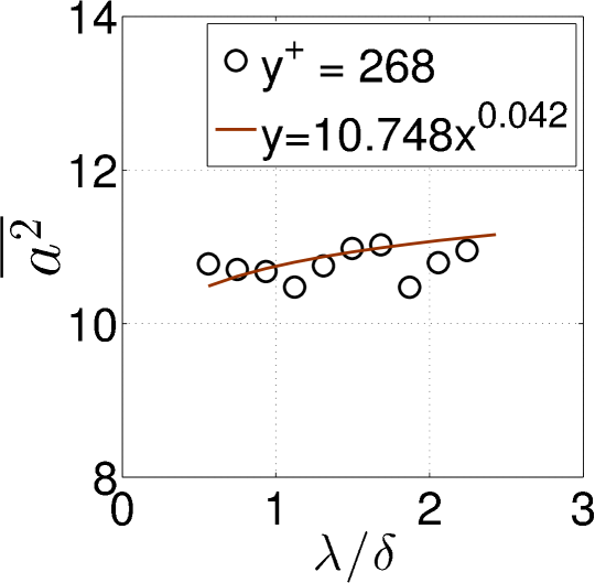
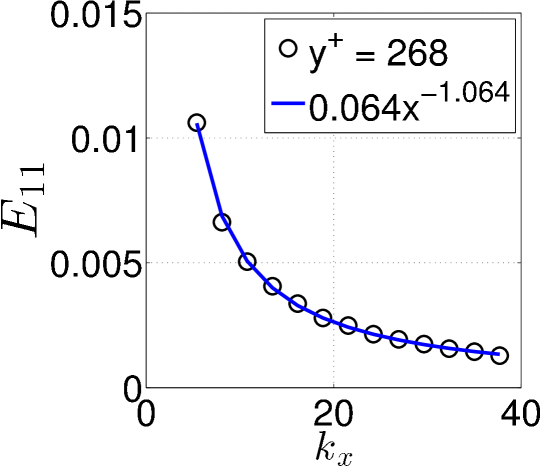
Figure 11: Lin-lin plots of $\overline{a^{2}}$ versus $\lambda/\delta$ (left) and streamwise energy spectra plotted at wall distances $y^{+}=$ 90, 158, 195 and 268 (from top to bottom) at $Re_{\theta}=20600$.

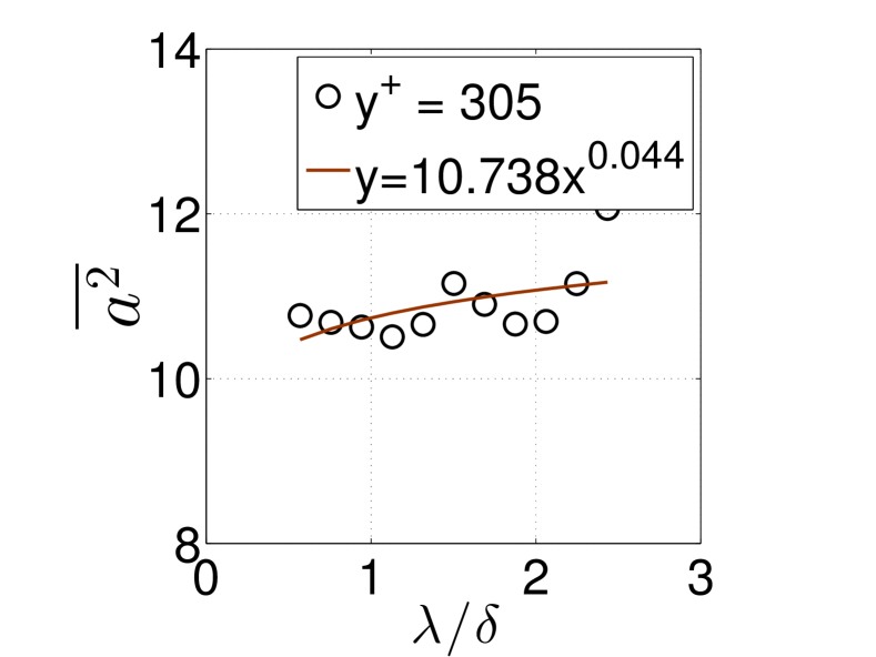
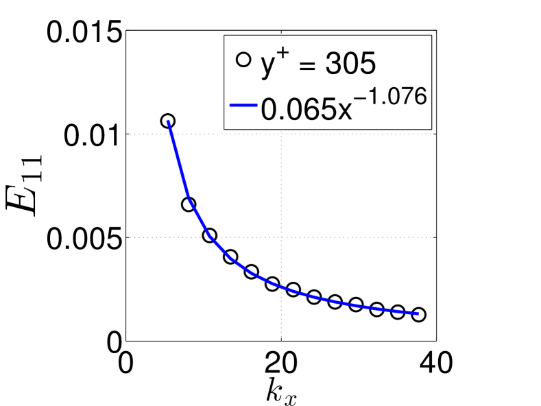
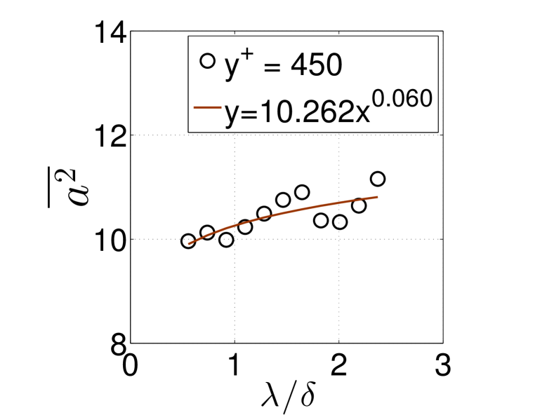
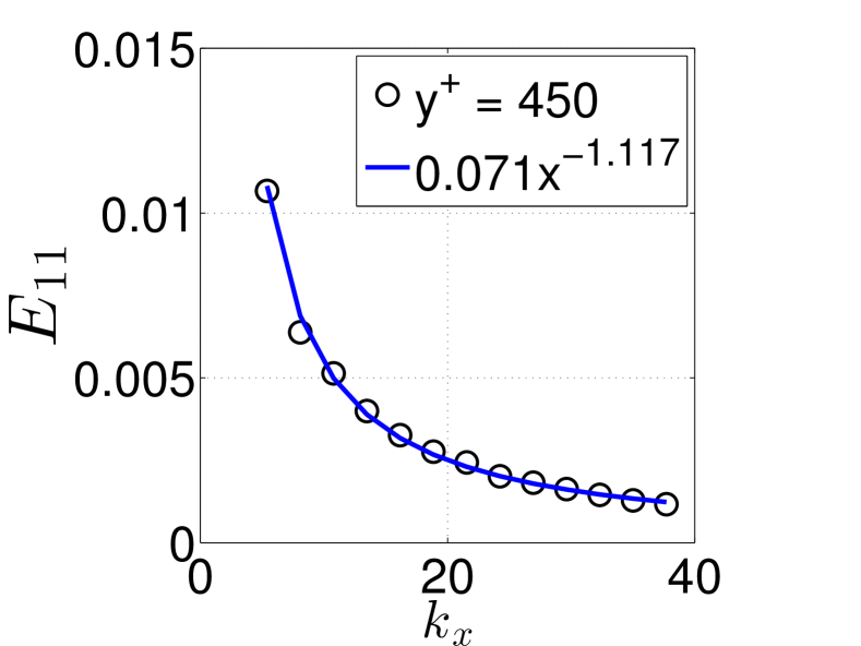
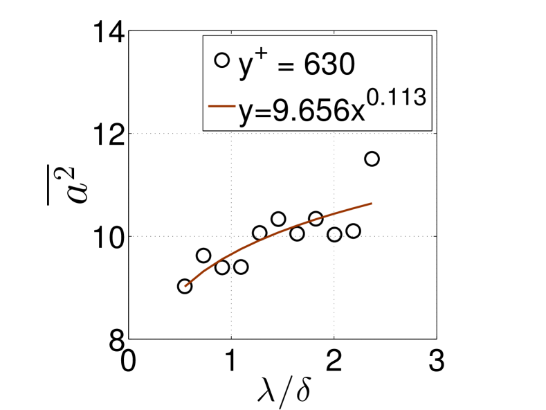
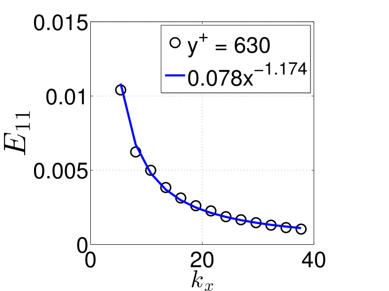
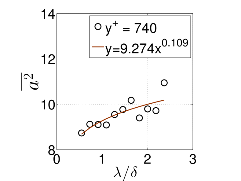
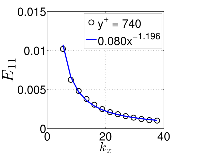
Figure 12: Lin-lin plots of $\overline{a^{2}}$ versus $\lambda/\delta$ (left) and streamwise energy spectra plotted at wall distances $y^{+}=$ 305, 450, 630 and 740 (from top to bottom) at $Re_{\theta}=20600$.

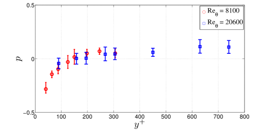
(a)
(b)
(c)

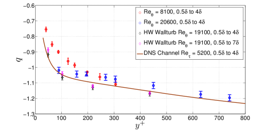
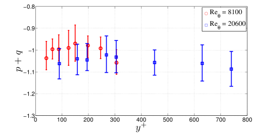
Figure 13: From top to bottom: (a) Exponents $p$ obtained from the best power-law fit of $\overline{a^{2}}\sim(\lambda/\delta)^{p}$. (b) Exponents $q$ obtained from the best power-law fit of $E_{11}\sim k_{x}^{q}$ for the present PIV data, the HWA turbulent boundary layer data of Tutkun et al. [tutkun09, ] (see figure 14(a) and the DNS of turbulent channel flow data of Lee & Moser [leemoser15, ] (see figure 14(b). (c) $p+q$ versus $y^{+}$. All these fits are obtained over the range of scales investigated in figures 9 to 12 (except for the HWA case in (b) where we have also included a fit over a range of length-scales extended up to $7\delta$). The resulting exponents are plotted with the $95$% confidence intervals for these fits.

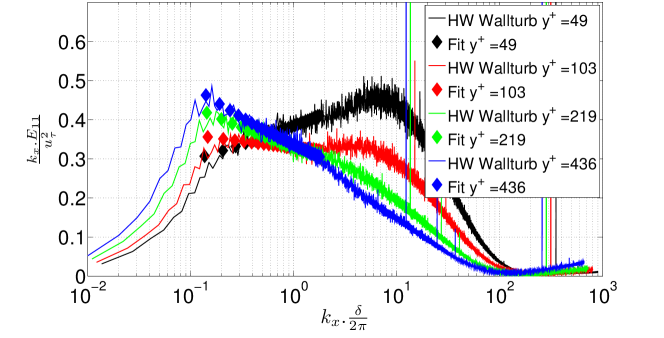
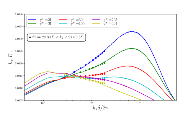
Figure 14: From top to bottom: (a) Lin-log plots of pre-multiplied streamwise energy spectra at selected wall distances obtained with HWA in the $Re_{\theta}=19100$ turbulent boundary layer of Tutkun et al. [tutkun09, ]. Least-square fits in a range bounded from above by $k_{x}\delta/(2\pi)=2$ but extended to wavenumbers as small as $k_{x}\delta/(2\pi)$ close to $10^{-1}$. (b) Lin-log plots of pre-multiplied streamwise energy spectra at selected wall distances from the $Re_{\tau}=5200$ turbulent channel flow DNS of Lee & Moser [leemoser15, ]. Least-square fits in the range $0.25\leq k_{x}/(2\pi)\leq 2$.

V.5 Discussion

It is important to stress that the support for (10)-(11) in figures 9 to 12 cannot be obtained without the crucial last step of our structure detection algorithm in subsection V.2 which discards structures that are not attached to the wall. The structures which do not touch the wall are in fact less elongated and less intense (i.e. smaller $\overline{a^{2}}$) on average. We have checked that if we only consider them, we do not find anything close to $p+q=-1$, i.e. (11).

The attached eddy concept introduced by Townsend [townsend1976structure, ] is therefore important for explaining $E_{11}(k_{x})$ but the results of our analysis suggest that the Townsend-Perry model does not hold without some significant corrections because the turbulent kinetic energy content in these wall-attached flow structures does not just scale with $U_{\tau}$. (If it did, $\overline{a^{2}}$ would scale with $U_{\tau}$ and $p$ would be uniformly 0.) At different $y$ inside such a structure, the level of turbulent kinetic energy depends both on $U_{\tau}$ and on the streamwise length of the structure at that height. Furthermore, this dependence varies with height: $\overline{a^{2}}$ decreases with increasing $\lambda/\delta$ very close to the wall, in the buffer layer, and increases with increasing $\lambda$ further up. As $\overline{a^{2}}$ transits smoothly from one dependence to the other, a particular height exists where $\overline{a^{2}}$ is independent of $\lambda$ and therefore depends only on $U_{\tau}$. At that very particular height, $E_{11}(k_{x})\sim k_{x}^{-1}$. However, strictly speaking, this is not a Townsend-Perry spectrum, it is just the spectrum at that particular distance from the wall where the turbulent kinetic energy inside the streaky structures transits from a decreasing to an increasing dependence on the length of these structures. Our conclusion agrees with Nickels et al. [nickels2007some, ] in their statement that it is necessary to take measurements close to the wall to observe a $k_{x}^{-1}$ behaviour, in fact at $y^{+}$ between $100$ and $200$ as they also found. However, these authors were not in possession of (10)-(11) and therefore did not measure $\overline{a^{2}}$ at various heights and for various values of $\lambda/\delta$ which now allows us to see that the $k_{x}^{-1}$ behaviour at the edge of the buffer layer is not the Townsend-Perry spectrum but just a transitional instance of a more involved spectral structure. In fact, the spectral picture which emerges from our analysis is a unified picture which brings together the buffer and inertial layers in a seemless way.

In figure 15 we plot examples of measured streamwise velocity fluctuations and the on-off signals with which we model them at various heights from the wall. Our model on-off signals are clearly a drastic simplification of the data but one gets the impression from these plots that they capture the sharpest gradients in the signal and therefore much of its spectral content at the length-scales considered here. The lengths of the non-zero parts of the model signals correspond to $\lambda$ and the actual values of the on-off signal in these non-zero parts correspond to the average value $\alpha$ of the streamwise fluctuating velocity component inside each part. We stress that it is enough that our on-off model agrees with the data in the way it does in figures 9 to 12 for a certain range of thresholds $u_{th}$ (see subsection V.2). Our model does not need to work for any arbitrary threshold; it only needs to work for those thresholds which effectively capture the spatial boundaries of the flow structure objects simulated by our on-off functions as mentioned at the end of the first paragraph of section II.

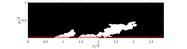
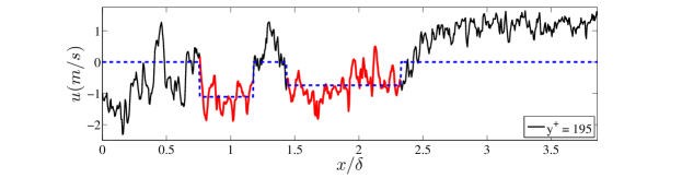
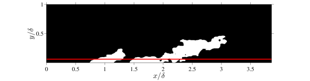
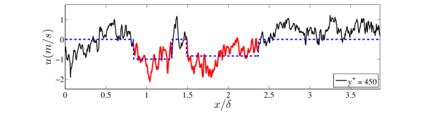
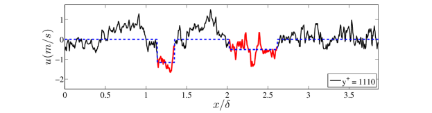
Figure 15: An example of a detected wall-attached flow structure for $Re_{\theta}=20600$ and the $u(x)$ signal through this structure at three different $y^{+}$ positions. The red line in the repeated binary image indicates the $y^{+}$ position where the signal $u(x)$ is recorded ($y^{+}=195,450,1110$). The black/red line in the $u(x)$ versus $x/\delta$ plots is the raw (un-filtered) PIV fluctuating streamwise fluctuating velocity outside/inside the detected flow structures. The dashed blue line is our model signal, equal to 0 outside and to the average value of $u$ inside the detected structures.

It is clear that a wider range of Reynolds numbers needs to be examined to establish the scalings of the lower and upper bounds of the range of wavenumbers where (10)-(11) holds. One might expect the upper bound to scale as $1/y$ because of the recent evidence (see Hultmark et al. [hultmark2012turbulent, ] and Laval et al. [laval2017comparison, ]) that a Townsend-like approximately logarithmic (or very weak power law) dependence on $y$ exists for the rms streamwise turbulent velocity in the outer part of the inertial range of wall-distances. If one assumes the lower bound to scale as $1/\delta$ and therefore an energy spectrum $E_{11}(k_{x})$ of the form (i) $E_{11}(k_{x})\sim U_{\tau}^{2}\delta$ for $0\leq k_{x}\leq B_{1}/\delta$, (ii) $E_{11}(k_{x})\sim U_{\tau}^{2}\delta(k_{x}\delta)^{-1-p}$ for $B_{1}/\delta\leq k_{x}\leq B_{2}/y$ (where $B_{1}$ and $B_{2}$ are dimensionless constants and $p$ may be a function of $y$ as in figure 13(a) and (iii) comparatively negligible energy at wavenumbers $k_{x}>B_{2}/y$, then we should have

$$(u^{\prime+})^{2}\sim 1+{B_{1}^{p}\over p}(B_{1}^{-p}-(B_{2}\delta/y)^{-p}).$$ (12)

This expression for $(u^{\prime+})^{2}$ tends to

$$(u^{\prime+})^{2}\sim 1+(\ln B_{1}-\ln(B_{2}\delta/y))$$ (13)

as $p\to 0$ which is the Townsend logarithmic dependence on $y$ corresponding to $p\equiv 0$ (see Townsend [townsend1976structure, ], Perry & Abell [perry1977asymptotic, ] and Perry et al [perry1986theoretical, ]) . This logarithmic dependence (13) results from the assumption that the upper bound of the range of wavenumbers where (10)-(11) may hold with $p\equiv 0$ scales as $1/y$. Slightly non-zero values of $p$ give slight deviations from this logarithmic dependence, of the form (12).

Using the values of $p$ obtained in this work and plotted versus $y^{+}$ in figure 13 for our two values of $Re_{\theta}$, it is not possible to fit (12) to the data in the lower plot of figure 1 from $y^{+}=41$ to $306$ in the $Re_{\theta}=8100$ case and from $y^{+}=90$ to $742$ in the $Re_{\theta}=20600$ case. These are the $y^{+}$ ranges where (10)-(11) has been established for our data and they should therefore also be the ranges where (12) holds if the spectral model of the previous paragraph is good enough. However, in spite of the three adjustable dimensionless constants ($B_{1}$, $B_{2}$ and an overall constant of proportionality), (12) cannot fit the entire $y^{+}$ range for which this model has been designed, that is a $y^{+}$ range which includes both the $p<0$ and the $p>0$ regions.

A most suspect part of the spectral model used to derive (12) is its low wavenumber part. Vassilicos et al. [vassilicos2015streamwise, ] showed that the second peak or plateau part of the $u^{\prime+}$ profile can be reproduced by a spectral range between the very low wavenumber range where $E_{11}(k_{x})\sim U_{\tau}^{2}\delta$ and the wavenumber range where $E_{11}(k_{x})\sim U_{\tau}^{2}\delta(k_{x}\delta)^{-1-p}$. In fact, Vassilicos et al. [vassilicos2015streamwise, ] also showed that this extra intermediate spectrum is necessary for a sufficiently fast growth of the integral scale with distance from the wall. A complete model of $E_{11}(k_{x})$ would therefore require the spectral range introduced by Vassilicos et al. [vassilicos2015streamwise, ] as well as the spectral range studied here.

VI Conclusion

We obtained well-resolved PIV data of a flat plate turbulent boundary layer in a large field of view at two Reynolds numbers, $Re_{\theta}=8100$ and $Re_{\theta}=20600$. A direct inspection of log-log plots of the streamwise energy spectrum would suggest $E_{11}(k_{x})\sim U_{\tau}^{2}k_{x}^{-1}$ in the range $2\pi/(4\delta)<k_{x}<0.63/y$. However, a closer look assisted by relation (10)-(11) reveals a significantly subtler behaviour. This relation introduces a specific data analysis which involves the extraction of wall-attached elongated streaky structures from PIV data. The concurrent analysis of streamwise energy spectra and of the relation between the turbulence levels inside streaky structures and the length of these structures offers strong support for (10)-(11) over a significant range of wavenumbers and length-scales. This range covers LSMs and is comparable to the range where one might have expected the Townsend-Perry attached eddy model spectra to be present. Even though $k_{x}^{-1}$ spectra are not, strictly speaking, validated by our data, the streaky structures which account for the scalings of $E_{11}(k_{x})$ do need to be wall-attached for relation (10)-(11) to hold. Our conclusions agree with the experiments of Vallikivi et al. [vallikivi2015spectral, ] which actually suggest that the Townsend-Perry $k_{x}^{-1}$ spectrum cannot be expected even at very high Reynolds numbers. The revised Townsend-Perry streamwise energy spectral form (10)-(11) with $p=p(y^{+})$ given by figure 13(a) appears to extend the validity of the attached eddy concept and its revised consequences to a wider range of Reynolds numbers and a wider range of wall distances.

Finally, we stress that relation (10)-(11) is predicated on these wall-attached streaky structures being space-filling, i.e. $D=1$ in the notation of section II. The pdf of the streamwise length of the educed streaky structures does indeed follow a power law with exponent $-1-D=-2$ over the range of scales which corresponds to the one where (10)-(11) holds.

Our work has shed some new light on the streamwise turbulence spectra of wall turbulence by revealing that some of the inner structure of wall-attached eddies is reflected in the scalings of these spectra via $p(y^{+})$. An important implication of this structure is that the friction velocity is not sufficient to scale the spectra. Future work must now further probe the inner structure of wall-attached eddies, attempt to explain it and extend our analysis to higher Reynolds numbers so as to establish with certainty the ranges of the power laws (exponents $p$ and $q$ in (10)-(11)) discussed in this paper. When this will be done, a complete picture of streamwise energy spectra will also need to integrate the spectral model of Vassilicos et al. [vassilicos2015streamwise, ].

Acknowledgements

The work was carried out within the framework of the CNRS Research Foundation on Ground Transport and Mobility, in articulation with the ELSAT2020 project supported by the European Community, the French Ministry of Higher Education and Research, the Hauts de France Regional Council. The authors gratefully acknowledge the support of these institutions. JCV also acknowledges the support of ERC Advanced Grant 320560.

Appendix A Effects of threshold levels and sign

Our results have no significant dependence on threshold $u_{th}$ in the range $-0.2u^{\prime}_{300^{+}}$ to $-0.6u^{\prime}_{300^{+}}$. An example of this lack of threshold dependence can be seen in the PDFs of $\lambda/\delta$ which we plot in figure 16. We also report in table 2 the number of structures educed by the algorithm described in subsection V.2 for the three negative threshold values $-0.2u^{\prime}_{300^{+}}$, $-0.4u^{\prime}_{300^{+}}$ and $-0.6u^{\prime}_{300^{+}}$. Figures 9 to 13 have been obtained for $u_{th}=-0.4u^{\prime}_{300^{+}}$ but we checked that they remain very similar without deviations from our conclusions if the threshold $u_{th}$ is chosen in the range $-0.2u^{\prime}_{300^{+}}$ to $-0.6u^{\prime}_{300^{+}}$.

$Re_{\theta}$	20600	8100
$-0.2u^{\prime}_{300^{+}}$	13517	17338
$-0.4u^{\prime}_{300^{+}}$	14493	19576
$-0.6u^{\prime}_{300^{+}}$	13366	19290

Table 2: Number of structures detected over a set of three negative thresholds for $Re_{\theta}=20600$ and $Re_{\theta}=8100$

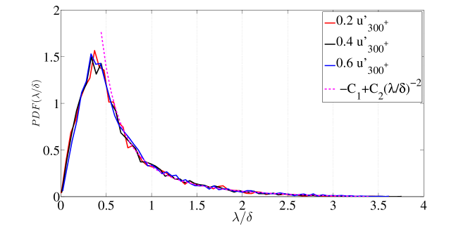
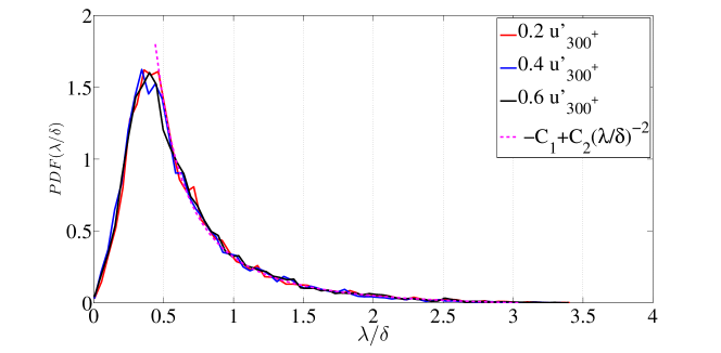
Figure 16: PDFs of streamwise lengths $\lambda$ of wall-attached structures at $y^{+}=195$ for $Re_{\theta}=20600$ (top) and $y^{+}=125$ for $Re_{\theta}=8100$ (bottom) over a set of thresholds

As mentioned in subsection V.2, this paper’s analysis can be repeated equally well on structures of positive streamwise fluctuating velocity. We provide examples of results obtained with $u_{th}=0.4u^{\prime}_{300^{+}}$ in figure 17 and table 3. There are indeed no significant differences in the results for the low and high speed attached flow regions, except for a lower but consistent value of $C_{1}$ and for a consistently lower value of $C_{2}$ in the lower $Re_{\theta}$ case. Figures 9 to 13 can be reproduced for this positive threshold $u_{th}=0.4u^{\prime}_{300^{+}}$ and show the exact same trend with $p$ increasing while $q$ is decreasing with increasing $y^{+}$. However, whereas $p$ takes values similar to those for $u_{th}=-0.4u^{\prime}_{300^{+}}$ in the lower $Re_{\theta}$ case, it does not do so in the higher $Re_{\theta}$ case. As a result $p+q$ is quite close to $-1$ in the lower $Re_{\theta}$ case but less so, and in fact closer to $-1.1$ on average, for the higher $Re_{\theta}$ (see figure 18).

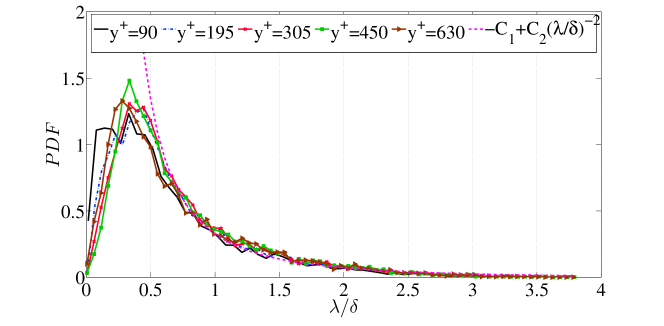
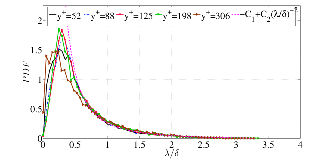
Figure 17: PDFs of streamwise lengths $\lambda$ of wall-attached structures of positive streamwise fluctuating velocity with $u_{th}=u^{\prime}_{300^{+}}$ at selected wall distances for $Re_{\theta}=20600$ (top) and $Re_{\theta}=8100$ (bottom). The fits shown here are for $y^{+}=195$ at $Re_{\theta}=20600$ and $y^{+}=198$ at $Re_{\theta}=8100$.

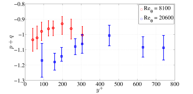
Figure 18: From top to bottom: (a) Exponents $p$ obtained from the best power-law fit of $\overline{a^{2}}\sim(\lambda/\delta)^{p}$. (b) $p+q$ versus $y^{+}$. These fits are obtained over the range of scales investigated for the high-speed regions and the resulting exponents are plotted with the $95$% confidence intervals for these fits. The $y^{+}$ positions and the two Reynolds numbers $Re_{\theta}$ are those in figures 9 to 12.

$Re_{\theta}$	20600					8100
$y^{+}$	90	195	305	450	630	52	88	125	198	306
$C_{1}$	0.02	0.02	0.01	0.02	0.02	0.02	0.02	0.02	0.03	0.02
$C_{2}$	0.35	0.36	0.34	0.38	0.37	0.28	0.29	0.28	0.31	0.29

Table 3: Values of the constants $C_{1}$ and $C_{2}$ in the form $-C_{1}+C_{2}(\lambda/\delta)^{-2}$ of the PDF of $\lambda/\delta$.

References

- (1) A. A. Townsend, “The structure of turbulent shear flow,” Cambridge UP, Cambridge(1976).
- (2) A. E. Perry and M. S. Chong, “On the mechanism of wall turbulence,” J. Fluid Mech. 119, 173–217 (1982).
- (3) A. E. Perry, S. Henbest, and M. S. Chong, “A theoretical and experimental study of wall turbulence,” J. Fluid Mech. 165, 163–199 (1986).
- (4) A. E. Perry and J. D. Li, “Experimental support for the attached-eddy hypothesis in zero-pressure-gradient turbulent boundary layers,” J. Fluid Mech. 218, 405–438 (1990).
- (5) I. Marusic, A. K. M. Uddin, and A. E. Perry, “Similarity law for the streamwise turbulence intensity in zero-pressure-gradient turbulent boundary layers,” Phys. Fluids 9, 3718–3726 (1997).
- (6) I. Marusic and G. J. Kunkel, “Streamwise turbulence intensity formulation for flat-plate boundary layers,” Phys. Fluids 15, 2461–2464 (2003).
- (7) A. E. Perry and C. J. Abell, “Asymptotic similarity of turbulence structures in smooth-and rough-walled pipes,” J. Fluid Mech. 79, 785–799 (1977).
- (8) T. B. Nickels, I. Marusic, S. Hafez, and M. S. Chong, “Evidence of the law in a high-Reynolds-number turbulent boundary layer,” Phys. Rev. Lett. 95, 074501 (2005).
- (9) T. B. Nickels, I. Marusic, S. Hafez, N. Hutchins, and M. S. Chong, “Some predictions of the attached eddy model for a high Reynolds number boundary layer,” Phil. Trans. R. Soc. Lond. 365, 807–822 (2007).
- (10) J. F. Morrison, B. J. McKeon, W. Jiang, and A. J. Smits, “Scaling of the streamwise velocity component in turbulent pipe flow,” J. Fluid Mech. 508, 99–131 (2004).
- (11) B. J. McKeon and J. F. Morrison, “Asymptotic scaling in turbulent pipe flow,” Phil. Trans. R. Soc. A 365, 771–787 (2007).
- (12) M. Vallikivi, B. Ganapathisubramani, and A. J. Smits, “Spectral scaling in boundary layers and pipes at very high Reynolds numbers,” J. Fluid Mech. 771, 303–326 (2015).
- (13) A. J. Smits, B. J. McKeon, and I. Marusic, “High-reynolds number wall turbulence,” Annu. Rev. Fluid Mech. 43, 353–375 (2011).
- (14) J. C. Vassilicos and J. C. R Hunt, “Fractal dimensions and spectra of interfaces with application to turbulence,” Proc. R. Soc. Lond. A. 435, 505–534 (1991).
- (15) J. Carlier and M. Stanislas, “Experimental study of eddy structures in a turbulent boundary layer using particle image velocimetry,” J. Fluid Mech. 535, 143 (2005).
- (16) J.-M. Foucaut, J. Carlier, and M. Stanislas, “PIV optimization for the study of turbulent flow using spectral analysis,” Meas. Sci. Technol. 15, 1046 (2004).
- (17) D. J. C. Dennis and T. B. Nickels, “Experimental measurement of large-scale three-dimensional structures in a turbulent boundary layer. Part 2. Long structures,” J. Fluid Mech. 673, 218–244 (2011).
- (18) L. S. G. Kovasznay, V. Kibens, and R. F. Blackwelder, “Large-scale motion in the intermittent region of a turbulent boundary layer,” J. Fluid Mech. 41, 283–325 (1970).
- (19) G. L. Brown and A. S. Thomas, “Large structure in a turbulent boundary layer,” Phys. Fluids 20, S243–S252 (1977).
- (20) N. Hutchins and I. Marusic, “Evidence of very long meandering features in the logarithmic region of turbulent boundary layers,” J. Fluid Mech. 579, 1–28 (2007).
- (21) D. J. C. Dennis and T. B. Nickels, “Experimental measurement of large-scale three-dimensional structures in a turbulent boundary layer. Part 1. Vortex packets,” J. Fluid Mech. 673, 180–217 (2011).
- (22) J. H. Lee and H. J. Sung, “Very-large-scale motions in a turbulent boundary layer,” J. Fluid Mech. 673, 80–120 (2011).
- (23) K. C. Kim and R. J. Adrian, “Very large-scale motion in the outer layer,” Phys. Fluids 11, 417–422 (1999).
- (24) M. Guala, S. E. Hommema, and R. J. Adrian, “Large-scale and very-large-scale motions in turbulent pipe flow,” J. Fluid Mech. 554, 521–542 (2006).
- (25) B. J. Balakumar and R. J. Adrian, “Large-and very-large-scale motions in channel and boundary-layer flows,” Phil. Trans. R. Soc. Lond. 365, 665–681 (2007).
- (26) M. Tutkun, W. K. George, J. Delville, M. Stanislas, P. B. V Johansson, J.-M Foucaut, and S. Coudert, “Two-point correlations in high reynolds number flat plate turbulent boundary layers,” Journal of Turbulence, N21(2009).
- (27) M. Lee and R. D. Moser, “Direct numerical simulation of turbulent channel flow up to 5200,” Journal of Fluid Mechanics 774, 395–415 (2015).
- (28) J. C. del Álamo, J. Jiménez, P. Zandonade, and R. D. Moser, “Scaling of the energy spectra of turbulent channels,” J. Fluid Mech. 500, 135–144 (2004).
- (29) M. Hultmark, M. Vallikivi, S. C. C. Bailey, and A. J. Smits, “Turbulent pipe flow at extreme Reynolds numbers,” Phys. Rev. Lett. 108, 094501 (2012).
- (30) J.-P. Laval, J. C. Vassilicos, J.-M. Foucaut, and M. Stanislas, “Comparison of turbulence profiles in high-Reynolds-number turbulent boundary layers and validation of a predictive model,” J. Fluid Mech. 814 (2017).
- (31) J. C. Vassilicos, J.-P. Laval, J.-M. Foucaut, and M. Stanislas, “The streamwise turbulence intensity in the intermediate layer of turbulent pipe flow,” J. Fluid Mech. 774, 324–341 (2015).