Stark resonance parameters for the $3a_{1}$ orbital of the water molecule

Abstract

The Stark resonance parameters for the $3a_{1}$ molecular orbital of H₂O are computed by solving a system of partial differential equations in spherical polar coordinates. The starting point of the calculation is the quantum potential derived for this orbital from a single-center expanded Hartree-Fock orbital. The resonance positions and widths are obtained after applying an exterior complex scaling technique to describe the ionization regime for external fields applied along the two distinct $\hat{z}$ directions associated with the symmetry axis. The procedure thus avoids the computation of multi-center integrals, yet takes into account the geometric shape of a simplified molecular orbital in the field-free case.

I Introduction

Despite the complexity that the multi-center nature of the water molecule entails, it has been the topic of numerous studies including laser-induced ionization and high-harmonic generation Farrell et al. (2011); Falge et al. (2010), as well as electron capture and ionization processes in ion-molecule collisions Murakami et al. (2012a, b); Luna et al. (2016); Gulyás et al. (2016); Hong et al. (2016); Errea et al. (2013a); Nandi et al. (2013); Errea et al. (2015). Most calculations are within the framework of the independent electron model and use a multi-center description of the potential Errea et al. (2013b, 2015). A strong motivation to continue exploring this subject comes from the fundamental role which ionization plays in radiation damage of biological tissue.

In a previous study of the H₂O valence orbitals exposed to strong dc fields, we used an approach to determine the resonance parameters for a given geometry of the orbitals without multi-center integrals Arias Laso and Horbatsch (2016). Based on the implementation of an exterior complex scaling method, a system of partial differential equations was solved numerically. The molecular potential was expressed as a spherically symmetric effective potential obtained from a single-center basis Hartree-Fock (HF) calculation Moccia (1964a). The ionization parameters for the $1b_{1}$ and $1b_{2}$ molecular orbitals were explored over a range of electric field strengths.

Here we extend the approach to study the dc Stark problem for the $3a_{1}$ molecular orbital of H₂O. Given the orientation of this orbital with respect to the plane in which the two protons are located it is deemed necessary to go beyond the spherical effective potential approximation which was used for the $1b_{1}$ and $1b_{2}$ orbitals. This is accomplished by deriving a potential $V_{\rm{eff}}(r,\theta)$ for the $3a_{1}$ orbital from the single-electron Schrödinger equation with HF orbital wavefunction and energy supplied as known quantities.

This paper is organized as follows: In Sec. II the construction of the effective potential $V_{\rm{eff}}(r,\theta)$ is presented. The required asymptotic corrections applied to the electronic potential are given in Sec. II.1, followed by a description of the problem in terms of a system of partial differential equations in Sec. II.2. Numerical results for the resonance parameters are presented in Sec. III, followed by conclusions in Sec. IV. Atomic units ($\hbar=m_{e}=e=4\pi\epsilon_{0}=1$) are used throughout.

II Non-spherical effective potential derived from molecular orbitals

The starting point for this work is the HF calculation of the H₂O molecule in a single-center Slater orbital basis Moccia (1964a). Previously, we used the dominant parts of the $1b_{1}$ and $1b_{2}$ orbitals, namely the $np_{x}$ and $np_{y}$ parts to derive spherically symmetric effective orbital-dependent potentials and applied a Latter correction to guarantee the proper asymptotic behavior for the respective potential Latter (1955); Arias Laso and Horbatsch (2016).

Applying the same procedure to the $3a_{1}$ orbtital, i.e., retaining the $np_{z}$ parts of the MO only leads again to a spherically symmetric effective potential. Since we are interested in the response of the orbital when applying an electric dc field along the symmetry axis (i.e., the $z-$axis), there is an obvious deficiency: the two protons (located in the $y-z$ plane) introduce a strong assymetry, which leads to significant admixtures of $s-$type Slater orbitals in the Moccia Slater-type orbitals (STO’s) Moccia (1964a).

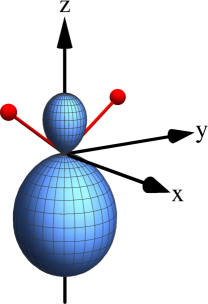
(a) Simplified $3a_{1}$ orbital

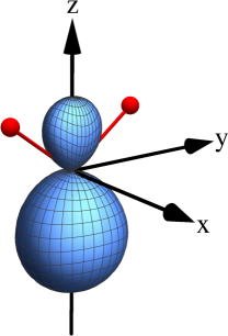
(b) Full Moccia $3a_{1}$ orbital

Figure 1: Schematic display of the $3a_{1}$ molecular orbital (shown in blue along the $z$ axis) used to construct $V_{\rm{eff}}(r,\theta)$. The orbital obtained from a reduced expansion in STO’s is shown in (1a), and the complete Moccia orbital is shown in (1b). Also indicated (in red in the $y-z$ plane) is the location of the protons. The $\hat{z}-$axis is the direction along which the external electric field of strength $F_{0}$ is applied.

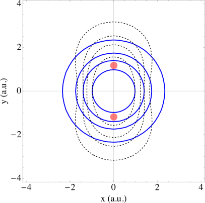
Figure 2: Projections of the probability densities for the $3a_{1}$ orbital on the $x-y$ plane. The simplified STO expansion is indicated as continuous blue lines, and the full Moccia expansion is indicated as black dashed lines. The protons are also indicated as red circles. The chosen contour values are $0.5,0.3,0.2,0.1$ starting from the innermost contour.

The proposed method to address this problem is to define a reduced single-center Moccia wave function,

$$\psi_{3a_{1}}(r,\theta)=\sum_{n,l}{c_{nl0}\varphi_{nl0}(r,\theta)}.$$ (1)

Here the $\varphi_{nl}(r,\theta)$ are Slater orbitals with $m=0$ for the magnetic quantum number, and we limited the expansion to STO’s of $2s$ and $2p_{z}$ type. The parameters are given in Table 1 and three $2p_{z}$ orbitals are mixed with three $2s-$type orbitals. This set of coefficients represents a reduced selection of the expansion parameters given by Moccia for the ground state of the water molecule Moccia (1964a) also shown in Table 1.

The probability densities for the $3a_{1}$ orbital as obtained from the reduced expansion (1) and from the Moccia self-consistent results are shown in Figures 1a and 1b respectively. The protons (in red) defined in the $y-z$ plane. As Fig. 1a indicates, the contributions to the density of the $2s-$type states reproduce the proper dependence of the $3a_{1}$ probability density with the polar angle $\theta$, as the broader hump is located on the negative $z$ axis in the same way that the complete Moccia representation illustrates in Fig. 1b.

In order to illustrate the fraction of the full Moccia expansion that our reduced wave function (1) represents, the projections of the probability densities over the $x-y$ plane are shown as contours of constant density in Figure 2, for the height where the protons are located. From the complete Moccia representation of the $3a_{1}$ MO (in dashed lines), one observes that the location of the protons (shown as red circles) has an influence on the shape of the upper lobe in the probability density, i.e., it introduces dependence on the azimuthal angle $\varphi$. In our simplified expansion, where only $l=0,1$ and $m=0$ symmetrical parts were included (shown with solid lines), the probability density misses to represent the proper azimuthal dependence that follows from the $m\neq 0$ parts.

The non-spherical effective potential corresponding to the STO expansion (1), $V_{\rm{eff}}(r,\theta)$, is obtained from the Schrödinger equation in spherical polar coordinates,

$$\left[-\frac{1}{2}\nabla^{2}+V_{\rm{eff}}(r,\theta)\right]\psi_{3a_{1}}(r,\theta)=E_{3a_{1}}\psi_{3a_{1}}(r,\theta).$$ (2)

For given $E_{3a_{1}}$ and $\psi_{3a_{1}}(r,\theta)$ it is straightforward to solve (2) for $V_{\rm{eff}}(r,\theta)$. In order to use this potential to define a Hamiltonian for the $3a_{1}$ orbital in an electric field an asymptotic Latter correction needs to be applied.

Table 1: Expansion coefficients and non-linear coefficients for the $3a_{1}$ MO. The parameters used in our reduced STO expansion are indicated as included.

$(n,l,m)$		$c_{nlm}$	$\zeta_{i}$
$(1,0,0)$	excluded	$-0.00848$	$12.600$
$(1,0,0)$	excluded	$0.08241$	$7.450$
$(2,1,0)$	included	$0.79979$	$1.510$
$(2,1,0)$	included	$0.00483$	$2.440$
$(2,1,0)$	included	$0.24413$	$3.920$
$(2,0,0)$	included	$-0.30752$	$2.200$
$(2,0,0)$	included	$-0.04132$	$3.240$
$(2,0,0)$	included	$0.14954$	$1.280$
$(3,2,0)$	excluded	$0.05935$	$1.600$
$(3,2,0)$	excluded	$0.00396$	$2.400$
$(3,2,2)$	excluded	$-0.09293$	$1.600$
$(3,2,2)$	excluded	$0.01706$	$2.400$
$(4,3,0)$	excluded	$-0.01929$	$1.950$
$(4,3,2)$	excluded	$-0.06593$	$1.950$

II.1 Interpolation and Latter correction of the effective potential

The non-central effective potential, $V_{\rm{eff}}(r,\theta)$, leads no longer to an orbital of $(l,m)$ symmetry, i.e., $2p_{z}$. This reflects the geometry of the problem as a consequence of the location of the protons. The use of this more general potential implies that the Latter criterium Latter (1955), which ensures the proper asymptotic behavior of the potential, is not as straightforward to implement as in the case of the spherical potential were the correction applies beyond a determined $r$ value Arias Laso and Horbatsch (2016). Now the correction must be implemented in the $r-\theta$ plane, by defining a $\theta-$dependent boundary beyond which the potential obtained from (2) rises above $-1/r$ in the asymptotic region.

We fix the $\theta$ coordinate at two extreme positions, such as $\theta=0$ and $\pi$, to find the corresponding $r$ values, $r_{0}$ and $r_{\pi}$, for which $V_{\rm{eff}}(r,\theta)=-1/r$ is satisfied, and then interpolate between them by introducing a $\theta-$dependent function. We use the function

$$r_{\rm{match}}(\theta) = \bar{r}-(r_{\pi}-\bar{r})\cos\theta,$$ (3)

where $\bar{r}=(r_{0}+r_{\pi})/2$. With this approach we redefine the effective potential to be the non-central potential derived from the reduced Moccia wave function using Eq. (2) when $r<r_{\rm{match}}(\theta)$, and $-1/r$ otherwise.

The weighted functions used to construct the Moccia orbitals Moccia (1964a) imply a potential difficulty in our problem. Since these functions are not exact solutions of the Schrödinger equation but were obtained from the variational principle by implementing a self-consistent calculation  Moccia (1964b), there may be regions in the $(r,\theta)$ domain where $\psi_{3a_{1}}(r,\theta)$ vanishes, whereas its second derivative remains finite; this produces a nodal line in the electronic potential. Thus finding a potential for which our approximate wave function satisfies a Schrödinger equation represents an intricate problem.

It turns out that the nodal region is so narrow that when solving the Schrödinger equation the kinetic energy term dominates and it is possible to obtain a solution that remains close to that obtained by the Hartree-Fock method Moccia (1964a), regardless of the fact that there is a region where the effective potential might diverge.

The probability density exhibits two humps indicating the positions of the protons, which is consistent with Figure 1, and the effects of the mixing with the $s-$state.

One may argue that one of the reasons this nodal region in the potential does not have a negative impact on the results is due to the way the $3a_{1}$ orbital responds to the effective potential by avoiding this region, its probability density being distributed as shown in Figure 3. We implement a numerical interpolation of $V_{\rm{eff}}(r,\theta)$ in order to ensure it continues smoothly over this problematic region.

The interpolation is achieved by collecting data from the evaluation of the potential on two sections of the $(r,\theta)$ grid in the vicinity of the nodal line, where the potential evaluates to finite values. Then a numerical interpolation was carried out between those regions in order to obtain a continuous function, $V_{\rm{eff}}^{\rm{intp}}(r,\theta)$, on the two-dimensional grid. The Latter correction is applied to the interpolated potential and the effective potential is defined according to (3):

$$V_{\rm{eff}}(r,\theta) = \left.\begin{cases}V_{\rm{eff}}^{\rm{intp}}(r,\theta)&\text{for }r<r_{\rm{match}}(\theta)\\ -1/r&\text{for }r>r_{\rm{match}}(\theta)\end{cases}\right\}.$$ (4)

Figure 3 shows the probability density for the $3a_{1}$ MO as a contour plot in the $r-\theta$ plane as obtained from the reduced Moccia expansion in Slater-type orbitals (1). Fig. 3 shows the same for the solution of the Schrödinger equation (2) using the interpolated $V_{\rm{eff}}(r,\theta)$, given in Eq. (4), with the Latter correction Latter (1955) applied in the asymptotic $r-$region.

[figure]style=plain,subcapbesideposition=top

[] []

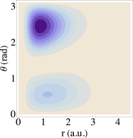
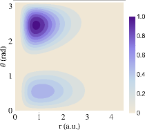
Figure 3: Contour plots of the probability density for the $3a_{1}$ molecular orbital. The orbital density constructed from the reduced STO expansion is shown in (3), while the solution obtained from the non-spherical $V_{\rm{eff}}(r,\theta)$ with Latter correction is shown in (3).

The effective potential (4) results in the probability density shown in Fig. 3 and yields an orbital energy of $-0.5579\ \rm{a.u.}$ for the $3a_{1}$ MO, with a relative change of $0.32\%$ in comparison with the self-consistent result of Moccia Moccia (1964a) of $-0.5561\ \rm{a.u.}$

As Fig. 3 indicates, the implementation of the Latter correction to the orbital-dependent potential obtained from Eq. (2), introduces a slight re-adjustment of the density, with a somewhat higher probability density in the region $0<\theta<\pi/2$. Since the Latter correction imposes an upper bound of $-1/r$ in the effective potential beyond some $\theta-$dependent boundary, this transformation in the effective potential establishes a softer tail for the orbital, which gives rise to the probability density re-distribution observed in Fig. 3 vs Fig. 3.

II.2 PDE in spherical polar coordinates

The problem of describing the ionization regime of the $3a_{1}$ MO under an external dc field applied along the orientation axis of the orbital is expressed in terms of a system of partial differential equations in spherical polar coordinates Arias Laso and Horbatsch (2016). A non-hermitian Hamiltonian is obtained as a result of applying exterior complex scaling Arias Laso and Horbatsch (2016); Aguilar and Combes (1971); Baslev and Combes (1971); Simon (1973, 1979) to the radial coordinate, where the $r-$coordinate is extended into the complex plane by the phase function $\chi(r)$, $r\to r\exp[i\chi(r)]$. The phase function $\chi(r)$ evolves smoothly from small values at $r=0$ to $\chi_{s}$ at large values of $r$ in the asymptotic region of the effective potential where the potential is spherically symmetric and purely Coulombic. The gradual increment of the scaling function is implemented by the same function as used in Arias Laso and Horbatsch (2016) as

$$\chi(r) = \frac{\chi_{\rm{s}}}{1+\exp[-\frac{1}{\Delta r}(r-r_{\rm{s}})]},$$ (5)

where the parameters $r_{\rm{s}}$ and $\Delta r$ were chosen for the function $\chi(r)$ to rise smoothly from nearly zero to $\chi_{\rm{s}}$ at $r-$values just outside where the Latter correction is applied, i.e., $r_{\rm{s}}>r_{\rm{match}}$.

Exterior complex scaling again leads to a system of coupled partial differential equations (6), where the $R(I)$ labels indicate the real and imaginary parts respectively due to the coordinate mapping into the complex plane.

$$-\frac{1}{2}\frac{\partial^{2}\psi_{R}}{\partial r^{2}}-\frac{1}{2r^{2}}(\frac{\cos\theta}{\sin\theta}\frac{\partial\psi_{R}}{\partial\theta}+\frac{\partial^{2}\psi_{R}}{\partial\theta^{2}})$$

$$+[\frac{m^{2}}{2r^{2}\sin^{2}\theta}+V_{\rm{eff}}^{R}(r,\theta)c_{2}-V_{\rm{eff}}^{I}(r,\theta)s_{2}-E_{R}c_{2}+E_{I}s_{2}+F_{0}r\cos\theta c_{3}]\psi_{R}$$

$$+[-V_{\rm{eff}}^{R}(r,\theta)s_{2}-V_{\rm{eff}}^{I}(r,\theta)c_{2}+E_{R}s_{2}+E_{I}c_{2}-F_{0}r\cos\theta s_{3}]\psi_{I} = 0,$$

$$\vspace{1cm}-\frac{1}{2}\frac{\partial^{2}\psi_{I}}{\partial r^{2}}-\frac{1}{2r^{2}}(\frac{\cos\theta}{\sin\theta}\frac{\partial\psi_{I}}{\partial\theta}+\frac{\partial^{2}\psi_{I}}{\partial\theta^{2}})$$

$$+[\frac{m^{2}}{2r^{2}\sin^{2}\theta}+V_{\rm{eff}}^{R}(r,\theta)c_{2}-V_{\rm{eff}}^{I}(r,\theta)s_{2}-E_{R}c_{2}+E_{I}s_{2}+F_{0}r\cos\theta c_{3}]\psi_{I}$$

$$+[V_{\rm{eff}}^{R}(r,\theta)s_{2}+V_{\rm{eff}}^{I}(r,\theta)c_{2}-E_{R}s_{2}-E_{I}c_{2}+F_{0}r\cos\theta s_{3}]\psi_{R} = 0.$$ (6)

The system of equations (6) was solved numerically on a two-dimensional grid defined in $(r,\theta)$ coordinates. The domains of $r$ and $\theta$ values were restricted to the intervals $r\in[\epsilon,r_{\rm{max}}]$ and $\theta\in[\eta,\theta_{\rm{max}}]$, with typical values $\epsilon=\eta=10^{-2}\ \rm{a.u.}$, $r_{\rm{max}}=28\ \rm{a.u.}$, and $\theta_{\rm{max}}=\pi-\eta$. In the limit of low field strengths, i.e., $F_{0}=0.05,0.06$, the value of $r_{\rm{max}}$ was increased to $40\ \rm{a.u.}$ in order to ensure the outer turning points lie inside the grid, as the tunneling barrier extends to larger $r$.

The problem of finding a solution of the Schrödinger equation for the $3a_{1}$ molecular orbital with contributions of $2s$ and $2p-$type states requires a set of boundary conditions that describes the properties of the orbital on the grid. In contrast with the $m=\pm\ 1$ solutions obtained for the $1b_{1}$ and $1b_{2}$ MO’s of H₂O Arias Laso and Horbatsch (2016), Neumann boundary conditions were implemented for the angular coordinate $\theta$ in order to obtain an eigenstate and orbital energy consistent with the variational results Moccia (1964a). This choice of boundary conditions, that the derivative with respect to $\theta$ vanishes at the limits of the mesh ($\theta=0$ and $\theta=\pi$), leads to solutions $\psi_{R(I)}(r,\theta)$ with a probability density consistent with the $\theta$ dependence of the $3a_{1}$ orbital, as shown in Figure 3. The physical parameters of interest, namely the resonance position, $E_{R}$, and width, $\Gamma=-2E_{I}$, that characterize the tunneling process of the quasi-stationary state when an external electric dc field is applied along the $\pm\hat{z}$ directions, were found by solving Eq. (6) for a set of field strength values, $F_{0}$, using a root search in order to find the energy that maximizes the probability density amplitude in the $2d-$grid.

III Stark resonance parameters

Results from applying the procedure described in Section II are shown in Figs. 4 and 5.

The resonance positions $E_{R}$ are shown in Figure 4 for external fields applied along the $\pm\hat{z}$ directions (red triangles/blue circles) for a range of external field strengths. For reference, the resonance positions obtained for the $1b_{1}$ and $1b_{2}$ MO’s using a spherically symmetric potential, $V_{\rm{eff}}(r)$, are also indicated in the form of dashed and dot-dashed lines respectively. For zero field strength $F_{0}=0$ self-consistent eigenenergies obtained by Moccia Moccia (1964a) are included as black crosses for the three valence orbitals of interest. As expected, the resonance position for the $3a_{1}$ orbital is bracketed by those for the $1b_{1}$ and $1b_{2}$ orbitals.

It can be noticed that for external fields applied along the $-\hat{z}$ direction, where most of the density is located, the field strength $F_{0}$ has to be strong, i.e., $F_{0}>0.1\ \rm{a.u.}$, for the resonance position to change appreciably. On the other hand, the resonance position for fields applied along $+\hat{z}$ appears to be more sensitive at weaker fields. However the barrier appears to be longer for external fields applied along the $+\hat{z}$ direction, at a field strength of about $F_{0}=0.25\ \rm{a.u.}$ the position values cross, indicating a higher sensitivity of the resonance positions for fields applied along the negative $\hat{z}$ direction as the field strength is increased further.

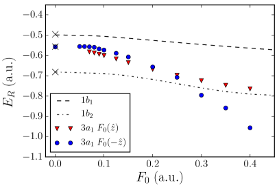
Figure 4: Resonance position in atomic units as a function of the external field strength $F_{0}$ and the orientation of the field, along the $\pm\hat{z}$ direction (red triangles/blue circles), for the $3a_{1}$ MO of H₂O. As a reference, the resonance position values for the $1b_{1}$ (dashed line) and $1b_{2}$ (dot-dashed line) MO’s are also included.

Figure 5 shows the resonance widths corresponding to external fields applied along the $\pm\hat{z}$ directions, as a function of the field strength $F_{0}$. The results obtained with a symmetric effective potential, $V_{\rm{eff}}(r)$, for the $1b_{1}$ and $1b_{2}$ MO’s are also shown as dashed and dot-dashed lines for comparison purposes.

In analogy to the $m=\pm 1$ orbitals, the ionization rates for the $3a_{1}$ MO, associated with the lifetime of the decaying state via $\Gamma\tau=1$, exhibit a threshold behavior at the weaker field strengths. Interestingly, for the two directions of the applied field, we find a lower critical field strength for the $3a_{1}$ orbital in comparison to what the more weakly bound orbital, $1b_{1}$, indicates. In the tunneling region, the $3a_{1}$ orbital for fields applied along the $-\hat{z}$ direction (blue squares) shows an ionization rate that is about one order of magnitude larger than the ionization rate for fields applied in the opposite direction (red triangles), this gap becomes narrower as the field strength increases toward the over-barrier regime.

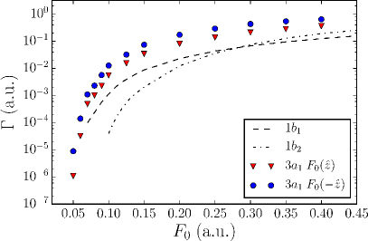
Figure 5: Resonance width in atomic units as a function of the external field strength $F_{0}$ and the orientation of the field, along the $\pm\hat{z}$ direction (red triangles/blue circles), for the $3a_{1}$ MO of H₂O. For reference, the resonance widths for the $1b_{1}$ (dashed line) and $1b_{2}$ (dot-dashed line) MO’s are also shown.

IV Conclusion

The Moccia single-center Hartree-Fock solution for the $3a_{1}$ orbital of H₂O has been investigated to understand its response to a strong external dc electric field. We generalized a method to obtain an effective potential to take into account $s-p$ type Slater orbital mixing included in the Moccia orbital. We ignored small $l>2$ and particularly $m=2$ contributions to limit the form of the effective potential to $V_{\rm{eff}}(r,\theta)$.

This permitted to study the relationship of the resonance parameters (position and width) to the neighboring valence orbitals $1b_{1}$ and $1b_{2}$ which were treated in a simplified approach before ($V_{\rm{eff}}(r)$ only, i.e., $1b_{1}\approx 2p_{x}$ and $1b_{2}\approx 2p_{y}$). Interestingly, the $3a_{1}$ orbital is found to ionize more easily than $1b_{1}$ or $1b_{2}$ irrespective of the field direction along $\hat{z}$. The work should serve as motivation for further studies of molecular orbitals of water using more sophisticated wave functions.