c-extremization from toric geometry

Abstract

We derive a geometric formulation of the 2d central charge $c_{r}$ from infinite families of 4d $\mathcal{N}=1$ superconformal field theories topologically twisted on constant curvature Riemann surfaces. They correspond to toric quiver gauge theories and are associated to D3 branes probing five dimensional Sasaki-Einstein geometries in the AdS/CFT correspondence. We show that $c_{r}$ can be expressed in terms of the areas of the toric diagram describing the moduli space of the 4d theory, both for toric geometries with smooth and singular horizons. We also study the relation between a-maximization in 4d and c-extremization in 2d, giving further evidences of the mixing of the baryonic symmetries with the exact R-current in two dimensions.

1 Introduction

Anomalies play a crucial role in the analysis of conformal field theories (CFTs). They provide consistency checks and impose several constraints on the existence of the IR fixed points and on the behavior of the RG flows. A well studied anomaly in 4d is the coefficient of the Euler density of $T_{\mu}^{\mu}$, referred as the central charge $a$. This quantity satisfies a c-theorem, decreasing between the endpoints of RG flows Cardy:1988cwa ; Komargodski:2011vj . When considering $\mathcal{N}=1$ supersymmetric CFTs (SCFTs), the central charge $a$, non perturbatively obtained in Anselmi:1997am , is maximized by the exact R–current of the superconformal algebra Intriligator:2003jj . The exact R–current is a linear combination of the trial UV R-current and the other global symmetries. By maximizing the central charge these mixing coefficients can be exactly computed.

The right–moving central charge $c_{r}$ of 2d $\mathcal{N}=(0,2)$ SCFTs satisfies a c–theorem as well Zamolodchikov:1986gt , and it is extremized by the exact 2d R–current Benini:2012cz . It is possible to construct classes of 2d SCFTs by the partial topological twist of 4d SCFTs on Riemann surfaces $\Sigma$ with constant curvature $2\kappa$ Witten:1988xj ; Bershadsky:1995vm . In order to preserve supersymmetry on the product space $\Sigma\times\mathbb{R}^{1,1}$ background magnetic fields for the global symmetries can be turned on Festuccia:2011ws ; Kutasov:2013ffl . These background fluxes must be properly quantized and cancel the contributions of the spin connection in the Killing spinor equations. For generic choices of the fluxes the 2d theory has $\mathcal{N}=(0,2)$ supersymmetry. The central charge of these 2d SCFTs can been computed from the global anomalies of the 4d theory Benini:2015bwz .

When considering 4d theories with an AdS₅ holographic dual description the topological twist can be reproduced at the gravitational level by turning on properly quantized fluxes for the (abelian) gauge symmetries in the bulk Maldacena:2000mw . This triggers a RG flow across dimensions that, when restricting to the supergravity approximation, connects the original AdS₅ description to a warped AdS${}_{3}\times\Sigma$ geometry.

Instead of constructing this flow one can consider the full 10d geometries. Solving the BPS equations in this case should lead to a warped product AdS${}_{3}\times\mathcal{M}_{7}$, where the general properties of the seven manifold $\mathcal{M}_{7}$ were originally discussed in Kim:2005ez ; Gauntlett:2007ts . This approach was taken in Benini:2015bwz for the infinite class of $Y^{pq}$ toric quiver gauge theories Benvenuti:2004dy . The $Y^{pq}$ theories are examples of 4d $\mathcal{N}=1$ SCFTs describing a stack of N D3 branes probing the tip of a toric Calabi–Yau threefold CY₃ over a 5d Sasaki–Einstein (SE) base X₅ with $U(1)^{3}$ isometry (see Kennaway:2007tq ; Franco:2017jeo and references therein).

An interesting aspect of toric gauge theories is the relation between the central charge $a$ and the volumes vol(X₅). It has been indeed shown that the holographic dictionary translates a–maximization into the minimization of vol(X₅) Martelli:2005tp . The equivalence between the two formulations has been derived explicitly in Butti:2005vn , where it was shown that the central charge can be obtained from the geometric data that describe the probed X₅ geometry and are related to the $U(1)^{3}$ isometry of X₅. Such data encode the structure of the moduli space of the 4d SCFT in a convex lattice polygon called the toric diagram.

A similar correspondence between the 2d central charge $c_{r}$ and the volumes of the seven manifolds is currently lacking. A possible obstruction in formulating a volume formula dual to c–extremization arises from the mixing of the global symmetries in the 2d exact R–current.

It is indeed possible to compare the structure of the mixing of the exact R–current with the abelian symmetries at the IR fixed point in the 4d $\mathcal{N}=1$ and in the 2d $\mathcal{N}=(0,2)$ theory obtained from twisted compactification. As a general result it has been observed that symmetries that trivially mix with the 4d R–current can mix non-trivially with the 2d one. This has been explicitly observed in Benini:2015bwz for the $Y^{pq}$ toric quiver gauge theories. In the 4d case the exact R–symmetry of toric quiver gauge theories is a mixture of the $U(1)^{3}$ symmetries of X₅. In the field theory language this can be rephrased as saying that the exact R–current is a mixing of the flavor symmetries that parameterize the mesonic moduli space and are encoded in the toric diagram. The other symmetries are of baryonic type. On the geometric side they are associated to the third Betti number of X₅. On the field theory side they correspond to the non-anomalous combination of the $U(1)\subset U(N)$ gauge groups, decoupling in the IR. In the case of X${}_{5}=Y^{pq}$ there is a single baryonic symmetry. It does not mix with the 4d R–current but it can mix in the 2d case Benini:2015bwz . This is expected to be a general behavior and should hold for models with a larger amount of baryonic symmetries.

This discussion leads to the conclusion that a putative volume formula for $c_{r}$ should involve symmetries that are not necessarily isometries of the seven manifold, so making the generalization of the results in Martelli:2005tp to these cases not straightforward.

In this paper, despite the role of the baryonic symmetries in c-extremization, we obtain an alternative formulation of $c_{r}$ in terms of the toric data of the 4d parent theory. The final formula involves the geometric data, the mixing parameters of the R–current with the other global symmetries and the fluxes turned on in the $\Sigma$ directions. At large $N$ our formulation reproduces the behavior of $c_{r}$ as a function of the mixing parameters and of the fluxes for toric quiver gauge theories topologically twisted on $\Sigma$.

The paper is organized as follows. In section 2 we review some basic aspects of toric quiver gauge theories and of the topological twist, necessary to our analysis. In section 3 we derive the expression of $c_{r}$ in terms of the toric data of the 4d theory. We first study cases with smooth horizons, correctly reproducing the behavior of $c_{r}$ as a function of the R-charges. We confirm the validity of this formula by studying many examples of increasing complexity. In section 4 we consider the case of non–smooth horizons, describing the prescription for obtaining $c_{r}$ in terms of the toric data of the 4d theory. In section 5 we study the compactification of del Pezzo gauge theories, dP₂ and dP₃, with respectively two and three non-anomalous baryonic symmetries, showing their mixing in the exact 2d R–current. Then we study a case with a generic amount of baryonic symmetries, by showing the mechanism in necklace quivers, denoted as $L^{pqp}$ theories. In section 6 we discuss the interpretation and possible implications of our results. For 2d theories obtained by topologically twisted reduction of dP₂ and dP₃ toric theories, in appendix A we report the explicit values for the parameters of $U(1)$ mixing for particular choices of the fluxes.

2 Review

We start our discussion by reviewing the main aspects of toric quiver gauge theories and their twisted compactification on constant curvature Riemann surfaces.

2.1 Toric quiver gauge theories

Toric quiver gauge theories Feng:2000mi describe the near horizon limit of a stack of N D3 branes probing the tip of a CY₃ cone over a 5d SE X₅, characterized by a $U(1)^{3}$ action on the metric. On the field theory side the dual ${\cal N}=1$ SCFTs are described by quiver gauge theories whose nodes carry $U(N)$ gauge factors and are connected by oriented arrows, representing bifundamental matter fields.

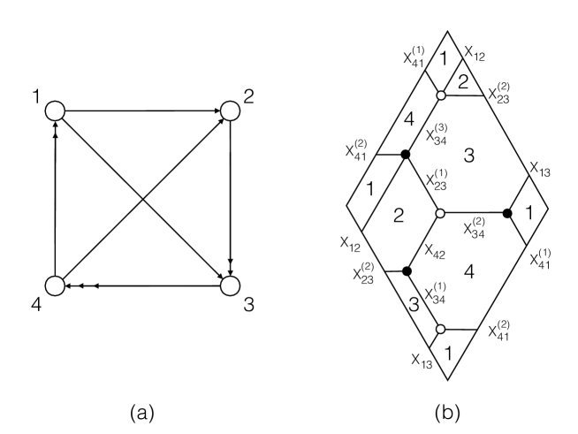
Figure 1: Quiver and dimer of the dP₁ model. In quiver (a) the number of arrows on the straight lines indicates the number of fields connecting two nodes.

In order to exemplify the discussion we consider the explicit case of a gauge theory living on a stack of N D3 branes probing the first del Pezzo singularity, dP₁. It has four gauge groups and the corresponding quiver is represented in Figure 1(a). The superpotential

$$W=-\epsilon_{\alpha\beta}X_{12}X_{23}^{(\alpha)}X_{34}^{(3)}X_{41}^{(\beta)}+\epsilon_{\alpha\beta}X_{23}^{(\alpha)}X_{34}^{(\beta)}X_{42}+\epsilon_{\alpha\beta}X_{13}X_{34}^{(\alpha)}X_{41}^{(\beta)}$$ (1)

is subject to the toric condition, which requires that each field appears in exactly two terms having opposite signs . This model has a $SU(2)\times U(1)$ flavor symmetry that, together with the $U(1)_{R}$ R–symmetry, builds up the isometry group of dP₁. In general, there are also baryonic symmetries associated to the non–trivial second cohomology group of X₅. These symmetries can be obtained from the $U(1)\subset U(N)$ gauge factors. They are IR free and at low energies decouple from the dynamics, becoming global symmetries. In quivers with a chiral–like matter content as the ones considered here, some of these $U(1)$’s are anomalous. The non–anomalous abelian factors correspond to the aforementioned baryonic symmetries. For the specific example of dP₁, to begin with there are four $U(1)_{i}\subset U(N)_{i}$ global symmetries of baryonic type with $T_{i=1,\dots,4}$ generators. Two combinations are anomalous and one decouples. We are then left with just a single non–anomalous baryonic symmetry that can be for example identified with the combination $2T_{1}-T_{2}+T_{3}$.

When flowing to the IR fixed point abelian flavor symmetries can mix with the R–current to form the exact R–symmetry, whereas the baryonic symmetries do not mix, as discussed in Bertolini:2004xf ; Butti:2005vn . This is a general feature of this family of 4d SCFTs.

For a quiver theory with $n_{G}$ gauge groups the mixing coefficients of global symmetries into the exact R–symmetries are obtained by maximizing the central charge Intriligator:2003jj

$$a_{FT}=\frac{3}{32}(3\,{\rm Tr}R^{3}-{\rm Tr}R)=\frac{3}{32}\big{(}2n_{G}(N^{2}-1)+\sum_{i=1}^{n_{F}}\text{dim}(\rho_{i})(3(R_{i}-1)^{3}-(R_{i}-1))\big{)}$$ (2)

where the first term is the contribution of the gaugini, $n_{F}$ it the total amount of matter multiplets, $\text{dim}(\rho_{i})$ is the dimension of the corresponding representation and $R_{i}$ the R–charge of the scalar component of the $i$–th multiplet. For matter multiplets in the bifundamental and/or adjoint representations, at large $N$ the central charge is further simplified by the constraint ${\rm Tr}R=0$ and we read

$$a_{FT}=\frac{9}{32}N^{2}\left(n_{G}+\sum_{i=1}^{n_{F}}(R_{i}-1)^{3}\right)+\mathcal{O}(1)$$ (3)

For toric gauge theories the $R_{i}$ charges can be determined directly from the geometric data of the singularity Gubser:1998vd ; Gubser:1998fp ; Martelli:2005tp ; Martelli:2006yb ; Tachikawa:2005tq ; Butti:2005vn ; Butti:2005ps ; Butti:2006nk ; Benvenuti:2006xg ; Lee:2006ru ; Kato:2006vx ; Gulotta:2008ef ; Eager:2010yu , as we now review.

First of all, we recollect how to construct the toric diagram corresponding to a given quiver gauge theory. One embeds the quiver diagram (for the dP₁ case see figure 1(a)) in a two dimensional torus. This resulting planar diagram can be dualized by inverting the role of faces and nodes, thus obtaining a bipartite diagram, called dimer, where faces correspond to gauge groups, edges to fields and nodes to superpotential interactions (for the dP₁ model it is given in figure 1(b)). The toric condition of the superpotential translates into a bipartite structure of the dimer. From the dimer one can construct perfect matchings (PM’s), that is collections of edges (fields) characterized by the property that each node is connected to one and only one edge of the set.

One can introduce a new set of formal variables $\pi_{I}$ associated to each PM. These variables are defined by the relations

$$X_{i}\equiv\prod_{I}(\pi_{I})^{M_{i,I}}$$ (4)

where the product is taken over all the PMs and

$$M_{i,I}=\left\{\begin{array}[]{ll}0&\text{if $X_{i}$ does not belong to the set of $\pi_{I}$}\\ 1&\text{if $X_{i}$ belongs to the set of $\pi_{I}$}\end{array}\right.$$ (5)

The $\pi_{I}$ provide a convenient set of variables that can be used to parametrize the abelian moduli space of the quiver gauge theory. The advantage of using the PMs variables $\pi_{I}$ instead of the more natural set of scalar components of the chiral fields $X_{i}$ comes from the fact that using definition (4) the F-term equations are trivially satisfied. This is a consequence of the fact that, in this basis, each term in the superpotential becomes equal to $\pm\prod_{I}\pi_{I}$, with $I$ ranging over all PMs.

To each PM we can associate a signed intersection number, $\pm 1$ or $0$, with respect to a basis of 1–cycles of the first homology of the torus. The signs can be inferred from the bipartite structure of the dimer. For each PM these two intersection numbers are the first two coordinates of 3d vectors $V_{I}\equiv(\cdot,\cdot,1)$ defining a convex integral polygon, named toric diagram, embedded into a 2d section of a 3d lattice at height one.

In the dP₁ case, the toric diagram is given by the 3d vectors $V_{I}$ that are associated to the PM’s as follows

$$\begin{array}[]{c|c|c|c}\text{PM}&\text{Primitive vector}&\text{PM}&\text{Primitive vector}\\ \hline\cr\pi_{1}=\{X_{34}^{(3)},X_{42},X_{13}\}&V_{1}=(1,0,1)&\pi_{5}=\{X_{12},X_{13},X_{42}\}&V_{5}=(0,0,1)\\ \pi_{2}=\{X_{23}^{(1)},X_{34}^{(1)},X_{41}^{(1)}\}&V_{2}=(0,1,1)&\pi_{6}=\{X_{13},X_{23}^{(1)},X_{23}^{(2)}\}&V_{6}=(0,0,1)\\ \pi_{3}=\{X_{12},X_{34}^{(1)},X_{34}^{(2)}\}&V_{3}=(-1,0,1)&\pi_{7}=\{X_{34}^{(1)},X_{34}^{(2)},X_{34}^{(3)}\}&V_{7}=(0,0,1)\\ \pi_{4}=\{X_{23}^{(2)},X_{34}^{(2)},X_{41}^{(2)}\}&V_{4}=(-1,-1,1)&\pi_{8}=\{X_{41}^{(1)},X_{41}^{(2)},X_{42}\}&V_{8}=(0,0,1)\\ \end{array}$$ (6)

and the corresponding toric diagram is drawn in figure 2(a).

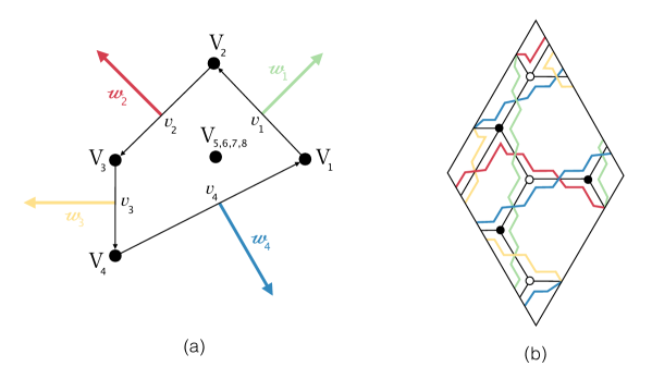
Figure 2: Toric diagram and tiling for the dP₁ model. In figure (a) primitive normal vectors $w_{I}$ of the toric diagram are also indicated and the different colors clarify their relation with the zig-zag paths in the dimer, figure (b). This is useful for reading the R-charges of the fields in terms of the charges of the zig-zag paths or of the PM.

It is also useful to review the notion of zig–zag paths. Given the set of primitive vectors $v_{I}$, one can define primitive normal vectors $w_{I}$, orthogonal to the edges of the toric diagram, $v_{I}\equiv(V_{I+1}-V_{I})$ (see figure 2(a)). These vectors are in 1–1 correspondence with a set of paths, made out of edges of the dimer, called zig–zag paths and represented in figure 2(b). They are oriented closed loops on the dimer that turn maximally left (right) at the black (white) nodes. The zig–zag paths correspond to differences of consecutive PM’s lying at the corners (and, if present, on the perimeter) of the toric diagram and are associated to the $U(1)$ global symmetries of the superpotential.

Viceversa, given a particular toric diagram it is possible to identify the main features of the corresponding quiver gauge theory as follows:

$\bullet$ The number of $U(N)$ gauge groups describing the quiver is given by twice the area of the toric diagram.

$\bullet$ The matter content of the theory (type of bifundamental fields and their degeneracy) can be inferred from the edges $v_{I}$ of the toric diagram Feng:2005gw , up to Seiberg duality, or equivalently toric phases, corresponding to Yang-Baxter transformations on the zig zag paths Hanany:2005ss . In its minimal toric phase a set of bifundamental fields $\Phi_{IJ}$ is assigned to each pair $(I,J)$ with degeneracy $|{\rm det}(v_{I},v_{J})|$.

$\bullet$ The corresponding spectrum of $R_{IJ}$ charges is determined by assigning a R–charge $\Delta_{\pi_{I}}$ to each external PM and using the following prescription Butti:2005ps

$$\left\{\begin{array}[]{lr}R_{IJ}=\sum_{K=I+1}^{J}\Delta_{\pi_{K}}&\quad I<J\vspace{.2cm}\\ R_{IJ}=2-\sum_{K=J+1}^{I}\Delta_{\pi_{K}}&\quad I>J\end{array}\right.$$ (7)

where the charges $\Delta_{\pi_{I}}$ are subject to the constraint

$$\sum_{I=1}^{d}\Delta_{\pi_{I}}=2$$ (8)

to ensure that each superpotential term has R–charge equal to two. A geometric interpretation of (8) can be given in terms of the isoradial embedding Hanany:2005ss .

The fact that the degeneracy of the fields with a given R–charge $R_{IJ}$ is given by $|{\rm det}(v_{I},v_{J})|$ has a nice geometric interpretation in terms of zig–zag paths Butti:2005ps .

$\bullet$ The number $d$ of external vertices of the toric diagram also determines the total number of non–anomalous $U(1)$ global symmetries of the gauge theory, which are identified as one R–symmetry, two flavor symmetries and $(d-3)$ baryonic symmetries. Analogously to (8), the condition for the superpotential to be neutral with respect to any non–R symmetry translates into

$$\sum_{I=1}^{d}Q_{\pi_{I}}^{\bf J}=0\qquad\quad{\bf J}=1,\dots,d-1$$ (9)

where $Q_{\pi_{I}}^{\bf J}$ is the charge of the $I$–th PM with respect to the ${\bf J}$–th symmetry.

$\bullet$ From the geometric data one can also identify the anomalies of the theory. The crucial observation is that the areas of the triangles of the toric diagram are related to the coefficients of the global anomalies of the field theory as Benvenuti:2006xg ; Lee:2006ru

$$\text{Tr}_{\rm 4d}({\cal T}_{I}{\cal T}_{J}{\cal T}_{K})=\frac{N^{2}}{2}|\det(V_{I},V_{J},V_{K})|$$ (10)

where ${\cal T}_{I}$ are global symmetry generators and the trace $\text{Tr}_{\rm 4d}$ is taken over the 4d fermions with the insertion of the 4d chirality operator.
Consequently, the central charge can be written as Lee:2006ru

$$a_{geom}\equiv\frac{9}{64}N^{2}\,|\det(V_{I},V_{J},V_{K})|\,\Delta_{\pi_{I}}\,\Delta_{\pi_{J}}\,\Delta_{\pi_{K}}$$ (11)

This expression is equivalent to (3) once we take into account the mapping between the two sets of $R_{i}$ and $\Delta_{\pi_{I}}$ charges, eq. (7).

In the case of the dP₁ model, using definition (4) we find the following map between fields $\Phi_{IJ}$ obtained from the toric diagram and those given by the quiver description

$$\begin{array}[]{c|c|c|c}(I,J)&|{\rm det}(v_{I},v_{J})|&\Phi_{IJ}&R_{IJ}\\ \hline\cr(4,1)&3&\{X_{13},X_{34}^{(3)},X_{42}\}&\Delta_{\pi_{1}}\\ (1,2)&2&\{X_{23}^{(1)},X_{41}^{(1)}\}&\Delta_{\pi_{2}}\\ (2,3)&1&\{X_{12}\}&\Delta_{\pi_{3}}\\ (3,4)&2&\{X_{23}^{(2)},X_{41}^{(2)}\}&\Delta_{\pi_{4}}\\ (1,3)&1&\{X_{34}^{(1)}\}&\Delta_{\pi_{2}}+\Delta_{\pi_{3}}\\ (2,4)&1&\{X_{34}^{(2)}\}&\Delta_{\pi_{3}}+\Delta_{\pi_{4}}\\ \end{array}$$ (12)

where $\Delta_{\pi_{I}}$ satisfy (8) and all internal PMs are assigned zero charge under all $U(1)$ symmetries.

The example we have considered has a smooth horizon where all the external points of the toric diagram correspond to corners. In this case the prescription for assigning R–charge to the bifundamental fields is unambiguously given in (7). In the case of singular horizons there are also points on the perimeter of the toric diagram that do not correspond to corners. These points have a degeneracy (given by a binomial coefficient), as they correspond to more than one PM. The assignment of the R–charges in terms of the external PM’s may then become ambiguous. According to the prescription in Butti:2005ps ; Butti:2006nk , at these points one sets to zero the R–charges of the PM’s that do not determine any zig-zag path, being then left with an unambiguous assignment of $\Delta_{\pi_{I}}$ charges.

The holographic correspondence provides the following relation between the central charge and the X₅ volume Gubser:1998vd

$$a_{\text{holo}}\equiv\frac{N^{2}\pi^{3}}{4\,\text{vol}(\text{X}_{5}(\mathbf{b}))}$$ (13)

where the volume is parameterized in terms of the components of the Reeb vector $\mathbf{b}$, a constant norm Killing vector that commutes with the X₅ isometries. It follows that the $a$-maximization prescription that determines the exact R–current in field theory corresponds to the volume minimization in the gravity dual.

When the cone over X₅ is toric the central charge can be directly obtained from the toric geometry. In fact, the X₅ volume can be expressed as Martelli:2005tp

$$\text{vol}(\text{X}_{5})=\frac{\pi}{6}\sum_{I=1}^{d}\text{vol}(\Sigma_{I})$$ (14)

where $d$ represents the number of vertices and vol$(\Sigma_{I})$ corresponds to the volume of a 3–cycle $\Sigma_{I}$, on which D3 branes, corresponding to dibaryons, are wrapped on Franco:2005sm .

Holographic data also determine the $\Delta_{\pi_{I}}$ charges that can be parameterized in terms of the components of the Reeb vector $\mathbf{b}$. Using the explicit parameterization Gubser:1998fp

$$\Delta_{\pi_{I}}(\mathbf{b})=\frac{\pi}{3}\frac{\text{vol}(\Sigma_{I}(\mathbf{b}))}{\text{vol}(\text{X}_{5}(\mathbf{b}))}$$ (15)

it is easy to show the equivalence between $a_{geom}$ in eq. (11) and $a_{\text{holo}}$ in eq. (13).

2.2 Twisted compactification

In this section we review the main aspects of partial topologically twisted compactifications of a 4d $\mathcal{N}=1$ SCFTs on a genus $g$ Riemann surface $\Sigma$, and the computation of the central charge $c_{r}$ for the corresponding 2d SCFTs, directly from 4d anomaly data.

When placing a 4d ${\cal N}=1$ SCFT on $\Sigma\times\mathbb{R}^{1,1}$, supersymmetry is generally broken by the coupling with the $\Sigma$ curvature. In order to (partially) preserve it one performs a twist Witten:1988xj by turning on background gauge fields along $\Sigma$ for an abelian 4d R–symmetry $t_{R}$ that assigns integer charges to the fields. Choosing its flux to be proportional to the curvature, its contribution to the Killing spinor equations cancels the contribution from the spin connection and possibly non–trivial solutions for Killing spinors can be found. More generally, one can also turn on properly quantized background fluxes along the $\Sigma$ directions for other abelian global symmetries. In this case supersymmetry is preserved if the associated gaugino variations vanish as well. Summarizing, the most general twist is performed along the generator

$$T=\kappa\,T_{R}+\sum_{{\bf I}=1}^{n_{A}}b_{\bf I}T_{\bf I}$$ (16)

where $\kappa=0$ for the torus and $\kappa=\pm 1$ for curved Riemann surfaces . Here $n_{A}$ refers to the number of abelian $T_{\bf I}$ generators of non–R global symmetries (both flavor and baryonic ones) and $b_{\bf I}$ are the corresponding background fluxes. For generic choices of the fluxes $\mathcal{N}=(0,2)$ supersymmetry is preserved on $\mathbb{R}^{1,1}$ Amariti:2017cyd .

After the twist the trial 2d R–symmetry generator is a mixture of the abelian generator $T_{R}$ and the other $T_{\bf I}$ generators

$$R=T_{R}+\sum_{{\bf I}=1}^{n_{A}}\epsilon_{\bf I}T_{\bf I}$$ (17)

where $\epsilon_{\bf I}$ are the mixing coefficients and $T_{R},T_{\bf I}$ are meant to act on fields reorganized in 2d representations.

At the IR fixed point the $\epsilon_{\bf I}$ coefficients have to extremize the 2d central charge $c_{r}=3k_{RR}\equiv 3{\rm Tr}_{\rm 2d}(RR)$ Benini:2013cda . Practically, the relevant anomaly coefficient $k_{RR}$ can be obtained from the anomaly polynomial $I_{6}$ expressed in terms of the triangular anomalies of the 4d theory, by integrating $I_{6}$ on $\Sigma$ and matching the resulting expression with the general structure of the anomaly polynomial $I_{4}$ in two dimensions Benini:2015bwz . In particular, one obtains the trial central charge

$$c_{r} = 3\,\eta_{\Sigma}\text{Tr}_{\rm 4d}(TR^{2})$$

$$= 3\,\eta_{\Sigma}\left[(b_{\bf K}k_{{\bf K}{\bf I}{\bf J}}+\kappa k_{R{\bf I}{\bf J}})\epsilon_{\bf I}\epsilon_{\bf J}+2(b_{\bf K}k_{R{\bf K}{\bf I}}+\kappa k_{RR{\bf I}})\epsilon_{\bf I}+(b_{\bf K}k_{RR{\bf K}}+\kappa k_{RRR})\right]$$

where $\eta_{\Sigma}=2|g-1|$ for $g\neq 1$ and $\eta_{\Sigma}=1$ for $g=1$, and we have defined $k_{{\bf K}{\bf I}{\bf J}}\equiv{\rm Tr}_{\rm 4d}(T_{\bf K}T_{\bf I}T_{\bf J})$, $k_{R{\bf I}{\bf J}}\equiv{\rm Tr}_{\rm 4d}(RT_{\bf I}T_{\bf J})$ and similarly for the other trace coefficients.

The exact central charge is finally obtained by extremizing with respect to the variables $\epsilon_{\bf I}$ Benini:2012cz . At the fixed point we have

$$\epsilon^{\ast}_{\bf I}=-\eta_{\Sigma}k^{-1}_{{\bf I}{\bf J}}\left(k_{R{\bf J}{\bf K}}b_{\bf K}+\kappa k_{RR{\bf J}}\right)$$ (19)

where

$$k_{{\bf I}{\bf J}}=\eta_{\Sigma}\left(\kappa k_{R{\bf I}{\bf J}}+b_{\bf K}k_{{\bf K}{\bf I}{\bf J}}\right)$$ (20)

From (19) we observe that coefficients $\epsilon^{\ast}_{\bf I}$ are generically non–vanishing for any choice of the $b_{\bf I}$ fluxes. In particular, this is true for the coefficients associated to baryonic symmetries, which then do mix with the exact R–current in two dimensions, even if they do not in the original 4d theory. This pattern has been already observed in Benini:2015bwz for the $Y^{pq}$ family. In section 5 we will study toric quiver gauge theories with a larger amount of baryonic symmetries, confirming that they generically mix with the 2d exact R–current after the twisted compactification on $\Sigma$.

Starting from a 4d toric theory with $n_{G}$ $U(N)$ gauge groups and $n_{F}$ massless chiral fermions, to each 2d field surviving the compactification on $\Sigma$ we can associate a $T$–charge $n_{i}$ and a R–charge $R_{i}$ according to (see eqs. (16) and (17))

$$n_{i}=\kappa\,r_{i}+Q_{i}^{\bf J}b_{\bf J},\quad R_{i}=r_{i}+Q_{i}^{\bf J}\epsilon_{\bf J}\qquad i=1,\dots,n_{F}$$ (21)

where $r_{i}$ is the R–charge respect to the 4d R–current and $Q_{i}^{\bf J}$ is the charge matrix of the fermions respect to the global $U(1)$ non–R symmetries, inherited from the 4d parent fields. Therefore, applying prescription (2.2) we find that at large $N$ the central charge before extremization is given by

$$c_{r}=3N^{2}\eta_{\Sigma}\left(\kappa\,n_{G}+\sum_{i=1}^{n_{F}}(n_{i}-\kappa)(R_{i}-1)^{2}\right)+{\cal O}(1)$$ (22)

This formula is general and applies to any 2d SCFT obtained from compactification of a 4d quiver gauge theory on a Riemann surface with curvature $\kappa$. Through $R_{i}$ it depends parametrically on the mixing coefficients $\epsilon_{\bf I}$ that need to be determined by the 2d extremization procedure.

As reviewed in the previous sub–section, in the case of 4d toric quiver theories we can parametrize the $U(1)$ charges in terms of PM variables $\Delta_{\pi_{I}}$ and $Q_{\pi_{I}}^{\bf J}$. When twisting, we can also assign to PMs a further $n_{\pi_{I}}$ charge with respect to the twisting $T$ symmetry (16) as (in this case $n_{A}=d-1$)

$$n_{\pi_{I}}=\kappa\Delta_{\pi_{I}}+b_{\bf J}Q^{\bf J}_{\pi_{I}}\quad\qquad{\rm with}\qquad\sum_{I=1}^{d}n_{\pi_{I}}=2\kappa$$ (23)

where the constraint on $n_{\pi_{I}}$ follows from (8) and (9).

The $r_{i}$ and $Q_{i}^{\bf J}$ charge assignments in two dimensions, eq. (21), need necessarily to respect the original constraints arising from the condition of superconformal invariance for the 4d superpotential. In particular, given the superpotential $W=\sum_{\alpha}W_{\alpha}$, these constraints imply that for each superpotential term $W_{\alpha}$ the conditions $\sum_{i\in W_{\alpha}}r_{i}=2$ and $\sum_{i\in W_{\alpha}}Q_{i}^{\bf J}=0$ hold. Consequently, from (21) we read

$$\sum_{i\in W_{\alpha}}R_{i}=2\,,\qquad\sum_{i\in W_{\alpha}}n_{i}=2\kappa$$ (24)

Now, we can think of the dimensional flow from the original 4d theory to the resulting 2d one as being accompanied by the set of toric data $(\Delta_{\pi_{I}},Q^{\bf J}_{\pi_{I}},n_{\pi_{I}})$ that parametrize the $U(1)$ charges in 4d and, consequently, that can still be used to parametrize the corresponding charges in two dimensions. Using this parametrization reinterpreted as charge parametrization for 2d fields, constraints (24) are traded with (8), (9) and (23).

3 $c_{r}$ from toric geometry

For the class of 2d SCFTs obtained from the topologically twist reduction of toric quiver gauge theories, we now provide a general prescription for determining the central charge $c_{r}$ directly in terms of the geometry of the toric diagram associated to the original 4d parent theory. This is the main result of the paper, which we are going to check in the successive sub–sections for a number of explicit examples.

3.1 Reading the 2d central charge from the toric diagram

To this end, we consider a toric gauge theory twisted along the abelian generator

$$T=\sum_{I=1}^{d}a_{I}{\cal T}_{I}\quad\qquad{\rm with}\qquad\sum_{I=1}^{d}a_{I}=2\kappa$$ (25)

where $I$ runs over the $d$ external points of the toric diagram. To be consistent with the conventions used so far, the abelian ${\cal T}_{I}$ generators are chosen to assign R–charge one to the superpotential of the 4d theory. It is always possible to construct such a set of generators by combining the generators of the 4d trial R–current, the two flavor symmetries and the $(d-3)$ non–anomalous baryonic symmetries that appear in (16). The new fluxes are subject to the constraint in (25) in order to ensure surviving ${\cal N}=(0,2)$ supersymmetry in 2d. They need to be further constrained in such a way that each flux $b_{\bf I}$ in (16) is properly quantized.

Accordingly, the 2d trial R–symmetry can be written as

$$R=\sum_{I=1}^{d}\epsilon_{I}{\cal T}_{I}\qquad{\rm with}\qquad\sum_{I=1}^{d}\epsilon_{I}=2$$ (26)

where the constraint follows from the requirement for $R$ to be a canonical normalized R–current.

The 2d central charge $c_{r}$ expressed in terms of the 4d anomaly coefficients $\text{Tr}_{\rm 4d}({\cal T}_{I}{\cal T}_{J}{\cal T}_{K})$, the $a_{I}$ fluxes and the mixing parameter $\epsilon_{I}$ becomes (see eq. (2.2))

$$c_{r}=3\,\eta_{\Sigma}\text{Tr}_{\rm 4d}(TR^{2})=3\,\eta_{\Sigma}\text{Tr}_{\rm 4d}({\cal T}_{I}{\cal T}_{J}{\cal T}_{K})\,a_{I}\epsilon_{J}\epsilon_{K}$$ (27)

In the case of toric theories the anomaly coefficients are given by (10) in terms of the areas of the triangles of the toric diagram. Therefore, the 2d central charge can be rewritten as

$$c_{r}=\frac{3\eta_{\Sigma}N^{2}}{2}|\det(V_{I},V_{J},V_{K})|a_{I}\epsilon_{J}\epsilon_{K}$$ (28)

In order to complete the map between the 2d field theory and the 4d geometric data we need to find a prescription for parametrizing the $a_{I}$ fluxes and the mixing parameters $\epsilon_{I}$ in terms of the PM’s associated to the external vertices of the toric diagram. To this end, we observe that the constraints satisfied by $a_{I}$ and $\epsilon_{I}$, eqs. (25, 26), are the same as the constraints satisfied by $\Delta_{\pi_{I}}$, eq. (8) and $n_{\pi_{I}}$, eq. (23). Therefore, we are naturally led to identify $\epsilon_{I}\equiv\Delta_{\pi_{I}}$ and $a_{I}\equiv n_{\pi_{I}}$. The central charge $c_{r}$ for the 2d SCFT obtained from a 4d toric quiver gauge theory topologically twisted on a 2d constant curvature Riemann surface can be then expressed entirely in terms of the toric data by the formula

$$c_{r}=\frac{3\eta_{\Sigma}N^{2}}{2}|\det(V_{I},V_{J},V_{K})|n_{\pi_{I}}\Delta_{\pi_{J}}\Delta_{\pi_{K}}$$ (29)

with $\Delta_{\pi_{J}}$ and $n_{\pi_{I}}$ satisfying constraint (8) and (23). The exact central charge for the 2d SCFT is then obtained by extremizing (29) as a function of $\Delta_{\pi_{I}}$.

Our proposal (29) requires some direct check on explicit examples that we report below. However, a holographical confirmation can be already found in the analysis of the AdS${}_{5}\to$ AdS₃ flow engineered in gauged supergravity Maldacena:2000mw . In this case we need to consider a consistent truncation of AdS${}_{5}\,\times X_{5}$, a 5d theory with a gravity multiplet, $n_{V}$ vector multiplets and $n_{H}$ hypermultiplets. The graviphoton plays the role of the R–symmetry current, while the $n_{V}$ vector multiplets correspond to the non–R global currents of the holographic dual field theory that remain as massless vector multiplets in a given truncation. In general $n_{V}\leq n_{A}$. The hypermultiplets impose the constraints on the global anomalies. When flowing to AdS₃ and using the Brown-Henneaux formula Brown:1986nw in this setup, it was observed Karndumri:2013iqa ; Benini:2013cda ; Amariti:2016mnz that $c_{r}$ can be expressed in terms of R–charges ${\hat{r}}^{I}$ and fluxes ${\hat{a}}^{J}$ as

$$c_{r}=\frac{2\pi^{3}N^{2}\eta_{\Sigma}}{3\text{vol}(\text{X}_{5})}C_{IJK}{\hat{a}}^{I}{\hat{r}}^{J}{\hat{r}}^{K}$$ (30)

where the constraints $\sum{\hat{r}}^{I}=2$ and $\sum{\hat{a}}^{I}=2\kappa$ need to be imposed. In this formula $C_{IJK}$ are the Chern–Simons coefficients of the dual supergravity, the R–charges ${\hat{r}}^{I}$ are obtained from the sections of the special geometry corresponding to the (constrained) scalars in the vector multiplets, and the prepotentials of $\mathcal{N}=2$ AdS₅ gauged supergravity. The constants ${\hat{a}}^{I}$ are the coefficients of the volume forms in the reduction of the 5d vector multiplets to 3d.

On the other hand, the $C_{IJK}$ coefficients are the holographic duals of the cubic ‘t Hooft anomaly coefficients, which for toric quiver gauge theories correspond to the areas of the triangles in the toric diagrams, eq. (10). Therefore

$$C_{IJK}=\frac{N^{2}}{2}|\det(V_{I},V_{J},V_{K})|$$ (31)

If we naturally identify the R–charges $\hat{r}^{I}$ with the $\Delta_{\pi_{I}}$ charges assigned to the PM’s, and similarly the $\hat{a}_{I}$ fluxes with the set of $n_{I}$ fluxes (they satisfy the same constraints $\sum\Delta_{\pi_{I}}=2$ and $\sum n_{\pi_{I}}=2\kappa$) we obtain our proposal (29).

3.2 Examples

In the remaining part of this section we test formula (29) on examples of increasing complexity. As a warm–up we consider the cases of X${}_{5}=S^{5}$ corresponding to $\mathcal{N}=4$ SYM and X${}_{5}=T^{1,1}$ corresponding to the conifold. Then we move to two more complicated cases, namely the second and third del Pezzo surfaces. We conclude the analysis by considering infinite families of quiver gauge theories associated to the $Y^{pq}$, $L^{pqr}$ and $X^{pq}$ geometries.

The strategy is the following. For each 4d model we use the general formula (22) to compute the central charge of the corresponding 2d SCFT obtained after twisted compactification. Then, we determine the parametrization of the R–charges and fluxes in terms of the toric data according to our prescription in section 3.1. Finally, we check that using this parametrization in (22) we obtain the central charge as given by (29).

$\mathcal{N}=4$ SYM

The first example that we consider corresponds to the case of X${}_{5}=S^{5}$. In this case the dual gauge theory is $\mathcal{N}=4$ SYM and its twisted compactification on a Riemann surface has been discussed in Benini:2012cz . The 4d field theory can be studied as a toric quiver gauge theory in $\mathcal{N}=1$ language. In this formulation the global symmetry corresponds to the $U(1)^{3}$ abelian subgroup of $SO(6)_{R}$. The quiver has a single node with three adjoint superfields $\Phi_{i}$ and superpotential

$$W=\Phi_{1}[\Phi_{2},\Phi_{3}]$$ (32)

The dimer, the zig-zag paths and the toric diagram are shown in Figure 3.

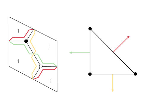
Figure 3: Dimer, zig-zag paths and toric diagram of $S^{5}$

By reducing this theory on $\Sigma$ the topological twist is performed along the $U(1)^{3}$ subgroup of the $SO(6)_{R}$. This corresponds to turning on three fluxes, one for each $U(1)$ factor, constraining their sum to be equal to the curvature $\kappa$. From the general expression (22) we can read the 2d central charge at large $N$

$$c_{r}=3N^{2}\eta_{\Sigma}\,\bigg{(}\kappa+\sum_{i=1}^{3}(n_{\Phi_{i}}-\kappa)(R_{\Phi_{i}}-1)^{2}\bigg{)}$$ (33)

where $R_{\Phi_{i}}$ are the R–charges and $n_{\Phi_{i}}$ the associated fluxes of the three adjoint fields. These variables are constrained by the relations $R_{\Phi_{1}}+R_{\Phi_{2}}+R_{\Phi_{3}}=2$ and $n_{\Phi_{1}}+n_{\Phi_{2}}+n_{\Phi_{3}}=2\kappa$.

Alternatively, we can compute the 2d central charge from (29) and find

$$c_{r}=3N^{2}\eta_{\Sigma}\big{(}n_{\pi_{1}}\Delta_{\pi_{2}}\Delta_{\pi_{3}}+n_{\pi_{2}}\Delta_{\pi_{3}}\Delta_{\pi_{1}}+n_{\pi_{3}}\Delta_{\pi_{1}}\Delta_{\pi_{2}}\big{)}$$ (34)

In order to check this result against (33) we need to express R–charges and fluxes in terms of the ones of the PM’s. This can be done with the prescription discussed in section 2.1. The three zig-zag paths in Figure 3 are the three possible combinations of two adjoints, $\Phi_{i}\Phi_{j}$. It follows that each adjoint field corresponds to the intersection of two primitive normal vectors $w_{I}$ of the toric diagram. Furthermore in this case each external PM corresponds to one of the adjoint fields. Therefore the charge and the flux assigned to each field correspond to the charge and the flux assigned to each external PM

$$\begin{array}[]{cccc}R_{\Phi_{1}}=\Delta_{\pi_{1}},&R_{\Phi_{2}}=\Delta_{\pi_{2}},&R_{\Phi_{3}}=\Delta_{\pi_{3}}\\ n_{\Phi_{1}}=n_{\pi_{1}},&n_{\Phi_{2}}=n_{\pi_{2}},&n_{\Phi_{3}}=n_{\pi_{3}}\end{array}$$ (35)

By substituting this parameterization in (33) we can easily prove that in this case the central charge is equivalent to (34) if constraints (8) and (23) are imposed.

The conifold

As a second example we study the case of the conifold, corresponding to X${}_{5}=T^{1,1}$. The model consists of a $SU(N)\times SU(N)$ gauge theory with two pairs of bifundamental $a_{i}$ and anti-bifundamental $b_{i}$ fields connecting the gauge groups and interacting through the superpotential

$$W=\epsilon_{ij}\epsilon_{lk}a_{i}b_{l}a_{j}b_{k}$$ (36)

The dimer, the zig-zag paths and the toric diagram are shown in Figure 4.

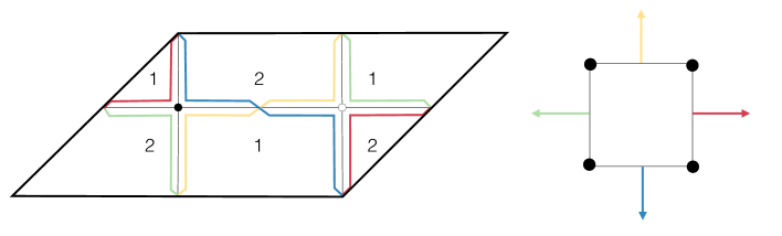
Figure 4: Dimer, zig-zag paths and toric diagram of $T^{1,1}$

In this case the flavor symmetry is $SU(2)^{2}$ and one baryonic $U(1)$ symmetry is also present. The R-charges of the four fields, $R_{a_{i}}$ and $R_{b_{i}}$ are constrained by $R_{a_{1}}+R_{a_{2}}+R_{b_{1}}+R_{b_{2}}=2$.

When twisting the theory on $\Sigma$ we introduce $T$–fluxes defined in (21). In this case they are $n_{a_{1}}$, $n_{a_{2}}$, $n_{b_{1}}$ and $n_{b_{2}}$, constrained by $n_{a_{1}}+n_{a_{2}}+n_{b_{1}}+n_{b_{2}}=2\kappa$.

The 2d central charge can be written at large $N$, using eq. (22)

$$c_{r}=3N^{2}\eta_{\Sigma}\,\bigg{[}2\kappa+\sum_{i=1}^{2}\bigg{(}(n_{a_{i}}-\kappa)(R_{a_{i}}-1)^{2}+(n_{b_{i}}-\kappa)(R_{b_{i}}-1)^{2}\bigg{)}\bigg{]}$$ (37)

This formula can be reproduced from the geometry of the toric diagram using prescription (29). To prove it, we start by ordering the vectors $V_{I}$ in the toric diagram as

$$V_{1}=(0,0,1),\quad V_{2}=(1,0,1),\quad V_{3}=(1,1,1)\quad V_{4}=(0,1,1)$$ (38)

The four zig–zag paths in Figure 4 are the four possible combinations of two bifundamentals, $a_{i}b_{j}$. It follows that each bifundamental field corresponds to the intersection of two consecutive primitive normal vectors of the toric diagram. Furthermore in this case each external PM corresponds to one of the bifundamental fields. Again the charge and the flux assigned to each bifundamental field correspond to the charge and the flux assigned to each external PM

$$\begin{array}[]{cccc}R_{a_{1}}=\Delta_{\pi_{1}},&R_{b_{1}}=\Delta_{\pi_{2}},&R_{a_{2}}=\Delta_{\pi_{3}},&R_{b_{2}}=\Delta_{\pi_{4}}\\ n_{a_{1}}=n_{\pi_{1}}&n_{b_{1}}=n_{\pi_{2}}&n_{a_{2}}=n_{\pi_{3}}&n_{b_{2}}=n_{\pi_{4}}\end{array}$$ (39)

By substituting parameterization (39) in (37) we can check directly that the central charge $c_{r}$ coincides with the one obtained from (29), under the conditions

$$\sum_{I=1}^{4}\Delta_{\pi_{I}}=2,\quad\quad\sum_{I=1}^{4}n_{\pi_{I}}=2\kappa$$ (40)

dP₂

We now consider the quiver gauge theory living on a stack of D3 branes probing the tip of the complex cone over dP₂ (see Benini:2015bwz for a discussion of the universal twist of dP_k theories). There are two Seiberg dual realizations of such a theory. Here we focus on the case with the minimal number of fields. This phase is usually referred to as the first phase and denoted as dP${}_{2}^{(I)}$. It is a quiver gauge theory (see figure 5) with five $SU(N)$ gauge groups and superpotential

$$W = X_{13}X_{34}X_{41}-Y_{12}X_{24}X_{41}+X_{12}X_{24}X_{45}Y_{51}-X_{13}X_{35}Y_{51}$$ (41)

$$+Y_{12}X_{23}X_{35}X_{51}-X_{12}X_{23}X_{34}X_{45}X_{51}.$$

The model has five non anomalous abelian global symmetries. There are a $U(1)_{R}$ symmetry and two $U(1)$ flavor symmetries corresponding to the $U(1)^{3}$ isometry of the SE geometry. There are also five baryonic currents: Two of them are non–anomalous, two are anomalous and one is redundant.

We perform the $c_{r}$ calculation from the geometry and we show the validity of formula (29) by matching the geometric result with the one obtained from the field theory analysis.

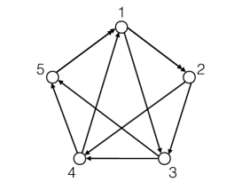
Figure 5: Quiver of the dP${}_{2}^{(I)}$ model

The dimer, the zig–zag paths and the toric diagram are shown in Figure 6.

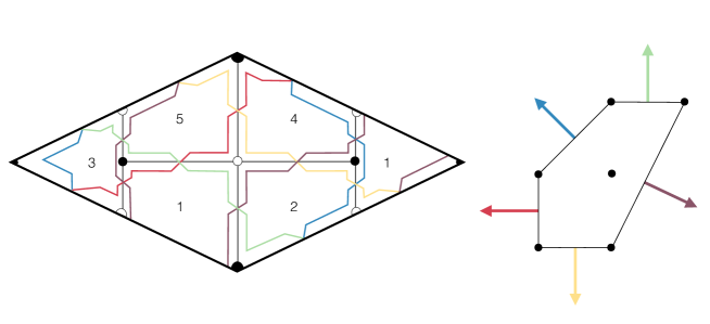
Figure 6: Dimer, zig-zag paths and toric diagram of dP₂.

The toric diagram is identified by the lattice points

$$V_{1}=(1,1,1)\quad V_{2}=(0,1,1)\quad V_{3}=(-1,0,1)\quad V_{4}=(-1,-1,1)\quad V_{5}=(0,-1,1)$$ (42)

The R–charges and the fluxes of the fields can be parameterized in terms of the $\Delta_{\pi_{I}}$ charges and the $n_{\pi_{I}}$ fluxes as

$$\begin{array}[]{l|cc}&\hskip 28.45274ptR_{\phi_{i}}&\hskip 28.45274ptn_{\phi_{i}}\\ \hline\cr\phi_{1}=X_{13}&\hskip 28.45274pt\Delta_{\pi_{4}}+\Delta_{\pi_{5}}&\hskip 28.45274ptn_{\pi_{4}}+n_{\pi_{5}}\\ \phi_{2}=X_{24}&\hskip 28.45274pt\Delta_{\pi_{5}}&\hskip 28.45274ptn_{\pi_{5}}\\ \phi_{3}=X_{51}&\hskip 28.45274pt\Delta_{\pi_{5}}&\hskip 28.45274ptn_{\pi_{5}}\\ \phi_{4}=X_{23}&\hskip 28.45274pt\Delta_{\pi_{2}}&\hskip 28.45274ptn_{\pi_{2}}\\ \phi_{5}=X_{41}&\hskip 28.45274pt\Delta_{\pi_{1}}+\Delta_{\pi_{2}}&\hskip 28.45274ptn_{\pi_{1}}+n_{\pi_{2}}\\ \phi_{6}=Y_{51}&\hskip 28.45274pt\Delta_{\pi_{2}}+\Delta_{\pi_{3}}&\hskip 28.45274ptn_{\pi_{2}}+n_{\pi_{3}}\\ \phi_{7}=Y_{12}&\hskip 28.45274pt\Delta_{\pi_{3}}+\Delta_{\pi_{4}}&\hskip 28.45274ptn_{\pi_{3}}+n_{\pi_{4}}\\ \phi_{8}=X_{45}&\hskip 28.45274pt\Delta_{\pi_{4}}&\hskip 28.45274ptn_{\pi_{4}}\\ \phi_{9}=X_{12}&\hskip 28.45274pt\Delta_{\pi_{1}}&\hskip 28.45274ptn_{\pi_{1}}\\ \phi_{10}=X_{35}&\hskip 28.45274pt\Delta_{\pi_{1}}&\hskip 28.45274ptn_{\pi_{1}}\\ \phi_{11}=X_{34}&\hskip 28.45274pt\Delta_{\pi_{3}}&\hskip 28.45274ptn_{\pi_{3}}\end{array}$$ (43)

subject to the constraints $\sum_{I=1}^{5}\Delta_{\pi_{I}}=2$ and $\sum_{I=1}^{5}n_{\pi_{I}}=2\kappa$. This parameterization satisfies the constraints $\sum_{a\in W}R_{\phi_{a}}=2$ and $\sum_{a\in W}n_{\phi_{a}}=2\kappa$. In this case there are $5$ gauge groups and the central charge is obtained from the formula

$$c_{r}=3N^{2}\eta_{\Sigma}\,\bigg{(}5\kappa+\sum_{i=1}^{11}(n_{\phi_{i}}-\kappa)(R_{\phi_{i}}-1)^{2}\bigg{)}$$ (44)

By substituting parameterization (43) in (44) we can see show that (44) is equivalent to (29) once the constraints (8) and (23) are imposed.

dP₃

Here we consider the quiver gauge theory living on a stack of D3 branes probing the tip of the complex cone over dP₃. There are four Seiberg dual realizations of such a theory, and we focus on the case with the minimal number of fields, usually called the first phase and denoted as dP${}_{3}^{(I)}$.

Figure 7: Quiver of the dP${}_{3}^{(I)}$ model

The quiver is represented in Figure 7, and it has six gauge groups. The superpotential is

$$W = X_{12}X_{24}X_{45}X_{51}-X_{24}X_{46}X_{62}+X_{23}X_{35}X_{56}X_{62}$$ (45)

$$- X_{35}X_{51}X_{13}+X_{34}X_{46}X_{61}X_{13}-X_{12}X_{23}X_{34}X_{45}X_{56}X_{61}.$$

The model possesses six non anomalous abelian global symmetries. There are a $U(1)_{R}$ symmetry and two $U(1)$ flavor symmetries corresponding to the $U(1)^{3}$ isometry of the SE geometry. There are also six baryonic currents:  Three are non–anomalous, two are anomalous and one is redundant. The dimer, the zig-zag paths and the toric diagram are shown in Figure 8.

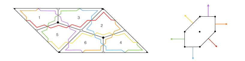
Figure 8: Dimer, zig-zag paths and toric diagram of dP₃

Again we can perform the calculation from the geometry, showing the validity of formula (29). The toric diagram is identified by the lattice points

$$V_{1}=(1,1,1)\quad\quad\,\,\,V_{2}=(0,1,1)\quad\,\,\,\,\,V_{3}=(-1,0,1)$$

$$V_{4}=(-1,-1,1)\quad V_{5}=(0,-1,1)\quad V_{6}=(1,0,1)$$ (46)

The R-charges and the fluxes of the fields can be parameterized in terms of the $\Delta_{\pi_{I}}$ charges and of the $n_{\pi_{I}}$ fluxes as

$$\begin{array}[]{l|cc}&\hskip 28.45274ptR_{\phi_{i}}&\hskip 28.45274ptn_{\phi_{i}}\\ \hline\cr\phi_{1}=X_{12}&\hskip 28.45274pt\Delta_{\pi_{6}}&\hskip 28.45274ptn_{\pi_{6}}\\ \phi_{2}=X_{13}&\hskip 28.45274pt\Delta_{\pi_{2}}+\Delta_{\pi_{3}}&\hskip 28.45274ptn_{\pi_{2}}+n_{\pi_{3}}\\ \phi_{3}=X_{23}&\hskip 28.45274pt\Delta_{\pi_{5}}&\hskip 28.45274ptn_{\pi_{5}}\\ \phi_{4}=X_{24}&\hskip 28.45274pt\Delta_{\pi_{1}}+\Delta_{\pi_{2}}&\hskip 28.45274ptn_{\pi_{1}}+n_{\pi_{2}}\\ \phi_{5}=X_{34}&\hskip 28.45274pt\Delta_{\pi_{4}}&\hskip 28.45274ptn_{\pi_{4}}\\ \phi_{6}=X_{35}&\hskip 28.45274pt\Delta_{\pi_{1}}+\Delta_{\pi_{6}}&\hskip 28.45274ptn_{\pi_{1}}+n_{\pi_{6}}\\ \phi_{7}=X_{45}&\hskip 28.45274pt\Delta_{\pi_{3}}&\hskip 28.45274ptn_{\pi_{3}}\\ \phi_{8}=X_{46}&\hskip 28.45274pt\Delta_{\pi_{5}}+\Delta_{\pi_{6}}&\hskip 28.45274ptn_{\pi_{5}}+n_{\pi_{6}}\\ \phi_{9}=X_{56}&\hskip 28.45274pt\Delta_{\pi_{2}}&\hskip 28.45274ptn_{\pi_{2}}\\ \phi_{10}=X_{51}&\hskip 28.45274pt\Delta_{\pi_{4}}+\Delta_{\pi_{5}}&\hskip 28.45274ptn_{\pi_{4}}+n_{\pi_{5}}\\ \phi_{11}=X_{61}&\hskip 28.45274pt\Delta_{\pi_{1}}&\hskip 28.45274ptn_{\pi_{1}}\\ \phi_{12}=X_{62}&\hskip 28.45274pt\Delta_{\pi_{3}}+\Delta_{\pi_{4}}&\hskip 28.45274ptn_{\pi_{3}}+n_{\pi_{4}}\\ \end{array}$$ (47)

with the constraints $\sum_{I=1}^{6}\Delta_{\pi_{I}}=2$ and $\sum_{I=1}^{6}n_{\pi_{I}}=2\kappa$. This parameterization satisfies the constraints $\sum_{a\in W}R_{\phi_{a}}=2$ and $\sum_{a\in W}n_{\phi_{a}}=2\kappa$. The central charge is obtained from the formula

$$c_{r}=3N^{2}\eta_{\Sigma}\,\bigg{(}6\kappa+\sum_{i=1}^{12}(n_{\phi_{i}}-\kappa)(R_{\phi_{i}}-1)^{2}\bigg{)}$$ (48)

By substituting parameterization (47) in (48) we can easily see that (48) is equivalent to (29) provided the constraints (8) and (23) are imposed.

$Y^{pq}$ theories

We can prove the validity of (29) also for infinite families of quiver gauge theories. The first family that we consider is X${}_{5}=Y^{pq}$. These models has been derived in Benvenuti:2004dy . They are quiver gauge theories with $2p$ gauge groups and bifundamental matter. For generic values of $p$ and $q$ the models have a $SU(2)\times U(1)$ flavor symmetry and one non-anomalous baryonic $U(1)$ symmetry. At the 2d fixed point this baryonic symmetry generically mixes with the R-current.

The general prescription to obtain the exact 2d central charge after twisted compactification has been given in Benini:2015bwz and detailed explicitly there for some cases of particular interest. Knowing the field content of these theories as summarized in Table (51), at large $N$ we can use the general formula (22) to write

$$c_{r}=3N^{2}\eta_{\Sigma}\,\bigg{(}2p\kappa+\sum_{i=1}^{6}d_{i}(n_{\phi_{i}}-\kappa)(R_{\phi_{i}}-1)^{2}\bigg{)}$$ (49)

We now show how to reproduce this expression from our geometric formulation (29).

For generic values of $p$ and $q$ the toric diagram has four external corners. There are also internal lattice points, associated to the anomalous baryonic symmetries, that do not play any role in our analysis. The corners of the toric diagram are associated to the vectors

$$V_{1}=(0,0,1),\quad V_{2}=(1,0,1),\quad V_{3}=(0,p,1)\quad V_{4}=(-1,p-q,1)$$ (50)

The parameterization of the R–charges and fluxes for the various fields in terms of the toric data can be read from the following table

$$\begin{array}[]{l|ccc}&\hskip 28.45274pt\text{multiplicity}&\hskip 28.45274ptR_{\phi_{i}}&\hskip 28.45274ptn_{\phi_{i}}\\ \hline\cr\phi_{1}=Y&\hskip 28.45274ptp+q&\hskip 28.45274pt\Delta_{\pi_{1}}&\hskip 28.45274ptn_{\pi_{1}}\\ \phi_{2}=U_{1}&\hskip 28.45274ptp&\hskip 28.45274pt\Delta_{\pi_{2}}&\hskip 28.45274ptn_{\pi_{2}}\\ \phi_{3}=Z&\hskip 28.45274ptp-q&\hskip 28.45274pt\Delta_{\pi_{3}}&\hskip 28.45274ptn_{\pi_{3}}\\ \phi_{4}=U_{2}&\hskip 28.45274ptp&\hskip 28.45274pt\Delta_{\pi_{4}}&\hskip 28.45274ptn_{\pi_{4}}\\ \phi_{5}=V_{1}&\hskip 28.45274ptq&\hskip 28.45274pt\Delta_{\pi_{2}}+\Delta_{\pi_{3}}&\hskip 28.45274ptn_{\pi_{2}}+n_{\pi_{3}}\\ \phi_{6}=V_{2}&\hskip 28.45274ptq&\hskip 28.45274pt\Delta_{\pi_{3}}+\Delta_{\pi_{4}}&\hskip 28.45274ptn_{\pi_{3}}+n_{\pi_{4}}\end{array}$$ (51)

The charges are subject to constraints (8). This parameterization satisfies the constraints $\sum_{a\in W}R_{\phi_{a}}=2$ and $\sum_{a\in W}n_{\phi_{a}}=2\kappa$ at each node of the dimer.

It is now easy to check that substituting these expressions for the R–charges and the fluxes in (49) and taking into account constraints (8) and (23) we reproduce exactly what we would obtain from (29).

$L^{pqr}$ theories

We now consider a second infinite family, corresponding to X${}_{5}=L^{pqr}$, for $p\neq r$ (the degenerate case $p=r$ will be treated in section 4). These models have been derived in Benvenuti:2005ja ; Butti:2005sw ; Franco:2005sm . They can be described in terms of a necklace quiver, i.e. a set of $p+q$ $SU(N)$ gauge groups such that each node is connected to its nearest neighbors by a bifundamental and an anti-bifundamental fields. In general there may be also additional adjoint chiral multiplets, depending on the value of $p$ and $q$ and on the Seiberg dual phase that we are considering.

The central charge at large $N$ can be easily obtained from (22) taking into account the field content of these theories in their the minimal phase, as summarized in table (54)

$$c_{r}=3N^{2}\eta_{\Sigma}\,\bigg{(}(p+q)\kappa+\sum_{i=1}^{6}d_{i}(n_{\phi_{i}}-\kappa)(R_{\phi_{i}}-1)^{2}\bigg{)}$$ (52)

To check the equivalence with the geometric prescrition (29) we first assign the external corners of the toric diagrams to the following vectors

$$V_{1}=(0,0,1),\quad V_{2}=(1,0,1),\quad V_{3}=(P,s,1)\quad V_{4}=(-k,q,1)$$ (53)

where $r-Ps-kq=0$ and $p+q=r+s$ and $p\leq r\leq q\leq s$. R-charges and fluxes parametrized in terms of the PM’s are

$$\begin{array}[]{l|ccc}&\hskip 28.45274pt\text{multiplicity}&\hskip 28.45274ptR_{\phi_{i}}&\hskip 28.45274ptn_{\phi_{i}}\\ \hline\cr\phi_{1}=Y&\hskip 28.45274ptq&\hskip 28.45274pt\Delta_{\pi_{1}}&\hskip 28.45274ptn_{\pi_{1}}\\ \phi_{2}=W_{2}&\hskip 28.45274pts&\hskip 28.45274pt\Delta_{\pi_{2}}&\hskip 28.45274ptn_{\pi_{2}}\\ \phi_{3}=Z&\hskip 28.45274ptp&\hskip 28.45274pt\Delta_{\pi_{3}}&\hskip 28.45274ptn_{\pi_{3}}\\ \phi_{4}=X_{1}&\hskip 28.45274ptr&\hskip 28.45274pt\Delta_{\pi_{4}}&\hskip 28.45274ptn_{\pi_{4}}\\ \phi_{5}=W_{1}&\hskip 28.45274ptq-s&\hskip 28.45274pt\Delta_{\pi_{2}}+\Delta_{\pi_{3}}&\hskip 28.45274ptn_{\pi_{2}}+n_{\pi_{3}}\\ \phi_{6}=X_{1}&\hskip 28.45274ptq-r&\hskip 28.45274pt\Delta_{\pi_{3}}+\Delta_{\pi_{4}}&\hskip 28.45274ptn_{\pi_{3}}+n_{\pi_{4}}\end{array}$$ (54)

with the constraints $\sum_{I=1}^{4}\Delta_{\pi_{I}}=2$ and $\sum_{I=1}^{4}n_{\pi_{I}}=2\kappa$. This parameterization satisfies the constraints $\sum_{a\in W}R_{\phi_{a}}=2$ and $\sum_{a\in W}n_{\phi_{a}}=2\kappa$.

Substituting this parameterization in (52) we directly obtain an expression equivalent to (29), once constraints (8) and (23) are taken into account.

$X^{pq}$ theories

Finally we consider the infinite family of models corresponding to X${}_{5}=X^{pq}$. They have been constructed in Hanany:2005hq . In this case there are $2p+1$ gauge groups and taking into account the spectrum of fields and their multiplicities as given in table (56), the 2d central charge as read from (22) is

$$c_{r}=3N^{2}\eta_{\Sigma}\,\bigg{(}(2p+1)\kappa+\sum_{i=1}^{10}d_{i}(n_{\phi_{i}}-\kappa)(R_{\phi_{i}}-1)^{2}\bigg{)}$$ (55)

To check it against the geometric calculation (22), we first label the external corners of the toric diagrams as (we take $p>q$)

$$V_{1}=(1,p,1),\quad V_{2}=(0,p-q+1,1),\quad V_{3}=(0,p-q,1)\quad V_{4}=(1,0,1)\quad V_{5}=(2,0,1)$$

The R-charges and fluxes parametrization in terms of the PM’s is given by

$$\begin{array}[]{l|ccc}&\hskip 28.45274pt\text{multiplicity}&\hskip 28.45274ptR_{\phi_{i}}&\hskip 28.45274ptn_{\phi_{i}}\\ \hline\cr\phi_{1}&\hskip 28.45274ptp+q-1&\hskip 28.45274pt\Delta_{\pi_{1}}&\hskip 28.45274ptn_{\pi_{1}}\\ \phi_{2}&\hskip 28.45274pt1&\hskip 28.45274pt\Delta_{\pi_{2}}&\hskip 28.45274ptn_{\pi_{2}}\\ \phi_{3}&\hskip 28.45274pt1&\hskip 28.45274pt\Delta_{\pi_{3}}&\hskip 28.45274ptn_{\pi_{3}}\\ \phi_{4}&\hskip 28.45274ptp-q&\hskip 28.45274pt\Delta_{\pi_{4}}&\hskip 28.45274ptn_{\pi_{4}}\\ \phi_{5}&\hskip 28.45274ptp&\hskip 28.45274pt\Delta_{\pi_{5}}&\hskip 28.45274ptn_{\pi_{5}}\\ \phi_{6}&\hskip 28.45274ptp-1&\hskip 28.45274pt\Delta_{\pi_{2}}+\Delta_{\pi_{3}}&\hskip 28.45274ptn_{\pi_{2}}+n_{\pi_{3}}\\ \phi_{7}&\hskip 28.45274pt1&\hskip 28.45274pt\Delta_{\pi_{3}}+\Delta_{\pi_{4}}&\hskip 28.45274ptn_{\pi_{3}}+n_{\pi_{4}}\\ \phi_{8}&\hskip 28.45274ptq-1&\hskip 28.45274pt\Delta_{\pi_{2}}+\Delta_{\pi_{3}}+\Delta_{\pi_{4}}&\hskip 28.45274ptn_{\pi_{2}}+n_{\pi_{3}}+n_{\pi_{4}}\\ \phi_{9}&\hskip 28.45274pt1&\hskip 28.45274pt\Delta_{\pi_{1}}+\Delta_{\pi_{2}}&\hskip 28.45274ptn_{\pi_{1}}+n_{\pi_{2}}\\ \phi_{10}&\hskip 28.45274ptq&\hskip 28.45274pt\Delta_{\pi_{4}}+\Delta_{\pi_{5}}&\hskip 28.45274ptn_{\pi_{4}}+n_{\pi_{5}}\\ \end{array}$$ (56)

with the constraints $\sum_{I=1}^{5}\Delta_{\pi_{I}}=2$ and $\sum_{I=1}^{5}n_{\pi_{I}}=2\kappa$. Once again, this parameterization satisfies the constraints $\sum_{a\in W}R_{\phi_{a}}=2$ and $\sum_{a\in W}n_{\phi_{a}}=2\kappa$.

Using this parameterization it is easy to check that result (55) is equivalent to (29), once constraints (8) and (23) are imposed.

4 Singular horizons and lattice points lying on the perimeter

In this section we discuss the case of toric diagrams with some external lattice points that are not corners but lie along the perimeter. These diagrams are associated to theories with non–smooth horizons, usually arising from the action of an orbifold.

In this case, as discussed in Butti:2005vn , the geometric procedure to extract the central charge $a$ from the toric diagram needs some modification. The reason is that the lattice points lying on the perimeter are associated to a multiple number of PM’s. Therefore, this requires a change in the prescription for assigning R–charges to the fields in terms of the charges of the PM’s.

The prescription that we propose follows the one described in Butti:2005ps and it works as follows. First divide the PM’s in two sets, the ones associated to corners of the toric diagram and the degenerate ones lying on the perimeter, namely $\pi^{c}$ and $\pi^{p}$ respectively. Then we associate a R–charge $\Delta_{\pi^{c}_{I}}$ to the PM’s at the corners, as done before. For the PM’s on the perimeter, instead, we proceed as follows. Observing that at each point on the perimeter only one of the degenerate PM’s enters the definition of the zig-zag paths, we assign a non zero charge $\Delta_{\pi^{p}_{I}}$ to this PM and set the charge of all the other PM’s associated to the same $I$-th lattice point to zero. With this modification of charge assignments we can then parameterize the R–charges $R_{i}$ and the fluxes $n_{i}$ unambiguously as described in section 3.

We have checked in a large set of examples that by applying this prescription the 2d central charge computed from the field theory analysis, eq. (22), matches with the one computed using formula (29). In the following we report the explicit check for a couple of examples in the $L^{pqp}$ class.

4.1 $L^{222}$

For this particular representative of the $L^{pqr}$ family the quiver diagram, the dimer with the zig–zag paths and the toric diagram are depicted in Figure 9. The superpotential of this model is

$$W=X_{12}X_{23}X_{32}X_{21}-X_{23}X_{34}X_{43}X_{32}+X_{34}X_{41}X_{14}X_{43}-X_{41}X_{12}X_{21}X_{14}$$ (57)

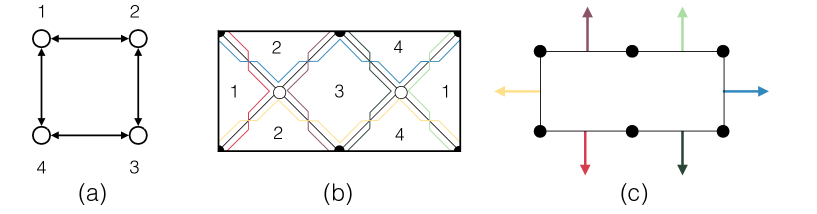
Figure 9: Dimer, zig zag paths and toric diagram of L²²²

The central charge can be obtained from formula (22) once we take into account the specific field content of the theory that can be read from the quiver diagram or in table (61). We obtain

$$c_{r}=3N^{2}\eta_{\Sigma}\,\bigg{(}4\kappa+\sum_{i=1}^{8}(n_{\phi_{i}}-\kappa)(R_{\phi_{i}}-1)^{2}\bigg{)}$$ (58)

In order to match this expression with (29) we first observe that the PM’s are related to the lattice points as follows

$$\begin{array}[]{c|c|c|c}\text{PM}&\text{Lattice point}&\text{PM}&\text{Lattice point}\\ \hline\cr\pi_{1}=\{X_{12},X_{34}\}&V_{1}=(0,0,1)&\pi_{2}=\{X_{21},X_{34}\}&V_{2}=(1,0,1)\\ \pi_{3}=\{X_{12},X_{43}\}&V_{2}=(1,0,1)&\pi_{4}=\{X_{21},X_{43}\}&V_{3}=(2,0,1)\\ \pi_{5}=\{X_{32},X_{14}\}&V_{4}=(2,1,1)&\pi_{6}=\{X_{32},X_{41}\}&V_{5}=(1,1,1)\\ \pi_{7}=\{X_{23},X_{14}\}&V_{5}=(1,1,1)&\pi_{8}=\{X_{23},X_{41}\}&V_{6}=(0,1,1)\\ \end{array}$$ (59)

The two points on the perimeter, identified as $V_{2}$ and $V_{5}$, are degenerate since they correspond to two different PM’s. As proposed in sub–section 3.1 we set the charges and the fluxes of one of the two PM’s of each degenerate point to zero. According to our prescription we set $\Delta_{\pi_{3}}=\Delta_{\pi_{7}}=0$ and $n_{\pi_{3}}=n_{\pi_{7}}=0$. The other non–vanishing charges and fluxes are constrained by the relations

$$\begin{array}[]{ccccccccccccc}\Delta_{\pi_{1}}&+&\Delta_{\pi_{2}}&+&\Delta_{\pi_{4}}&+&\Delta_{\pi_{5}}&+&\Delta_{\pi_{6}}&+&\Delta_{\pi_{8}}&=&2\\ n_{\pi_{1}}&+&n_{\pi_{2}}&+&n_{\pi_{4}}&+&n_{\pi_{5}}&+&n_{\pi_{6}}&+&n_{\pi_{8}}&=&2\kappa\end{array}$$ (60)

From here we can read the charges and the fluxes of every single field

$$\begin{array}[]{c|cc}&\hskip 28.45274ptR_{\phi_{i}}&\hskip 28.45274ptn_{\phi_{i}}\\ \hline\cr\phi_{1}=X_{12}&\hskip 28.45274pt\Delta_{\pi_{1}}&\hskip 28.45274ptn_{\pi_{1}}\\ \phi_{2}=X_{21}&\hskip 28.45274pt\Delta_{\pi_{4}}+\Delta_{\pi_{2}}&\hskip 28.45274ptn_{\pi_{4}}+n_{\pi_{2}}\\ \phi_{3}=X_{23}&\hskip 28.45274pt\Delta_{\pi_{8}}&\hskip 28.45274ptn_{\pi_{8}}\\ \phi_{4}=X_{32}&\hskip 28.45274pt\Delta_{\pi_{5}}+\Delta_{\pi_{6}}&\hskip 28.45274ptn_{\pi_{5}}+n_{\pi_{6}}\\ \phi_{5}=X_{34}&\hskip 28.45274pt\Delta_{\pi_{1}}+\Delta_{\pi_{2}}&\hskip 28.45274ptn_{\pi_{1}}+n_{\pi_{2}}\\ \phi_{6}=X_{43}&\hskip 28.45274pt\Delta_{\pi_{4}}&\hskip 28.45274ptn_{\pi_{4}}\\ \phi_{7}=X_{41}&\hskip 28.45274pt\Delta_{\pi_{6}}+\Delta_{\pi_{8}}&\hskip 28.45274ptn_{\pi_{6}}+n_{\pi_{8}}\\ \phi_{8}=X_{14}&\hskip 28.45274pt\Delta_{\pi_{5}}&\hskip 28.45274ptn_{\pi_{5}}\end{array}$$ (61)

This parameterization satisfies the constraints $\sum_{a\in W}R_{\phi_{a}}=2$ and $\sum_{a\in W}n_{\phi_{a}}=2\kappa$.

By substituting this parametrization in (58) we can easily prove that it is equivalent to (29) once constraints (60) are imposed.

4.2 $L^{131}$

As a second example, we consider the $L^{131}$ model associated to the quiver, dimer and toric diagram drawn in Figure 10. In this case the superpotential reads

$$W = X_{12}X_{21}X_{14}X_{41}-X_{12}X_{22}X_{21}+X_{32}X_{22}X_{23}$$ (62)

$$- X_{23}X_{33}X_{32}+X_{43}X_{33}X_{34}-X_{14}X_{43}X_{34}X_{41}$$

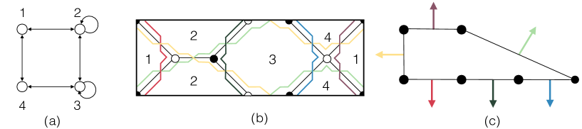
Figure 10: Dimer, zig-zag paths and toric diagram of L¹³¹

Given the particular field content, the central charge computed from (22) reads

$$c_{r}=3N^{2}\eta_{\Sigma}\,\bigg{(}4\kappa+\sum_{i=1}^{10}(n_{\phi_{i}}-\kappa)(R_{\phi_{i}}-1)^{2}\bigg{)}$$ (63)

In this case the PM’s are related to the lattice points as follows

$$\begin{array}[]{c|c|c|c}\text{PM}&\text{Lattice point}&\text{PM}&\text{Lattice point}\\ \hline\cr\pi_{1}=\{X_{12},X_{23},X_{34}\}&V_{1}=(0,0,1)&\pi_{2}=\{X_{21},X_{23},X_{34}\}&V_{2}=(1,0,1)\\ \pi_{3}=\{X_{12},X_{32},X_{34}\}&V_{2}=(1,0,1)&\pi_{4}=\{X_{12},X_{23},X_{43}\}&V_{2}=(1,0,1)\\ \pi_{5}=\{X_{21},X_{32},X_{34}\}&V_{3}=(2,0,1)&\pi_{6}=\{X_{21},X_{23},X_{43}\}&V_{3}=(2,0,1)\\ \pi_{7}=\{X_{12},X_{32},X_{43}\}&V_{3}=(2,0,1)&\pi_{8}=\{X_{21},X_{32},X_{43}\}&V_{4}=(3,0,1)\\ \pi_{9}=\{X_{14},X_{22},X_{33}\}&V_{5}=(1,1,1)&\pi_{10}=\{X_{41},X_{22},X_{33}\}&V_{6}=(0,1,1)\end{array}$$ (64)

There are still two perimeter points, this time with degeneracy three. According to our prescription described in sub–section 3.1 we set $\Delta_{\pi_{2}}=\Delta_{\pi_{3}}=\Delta_{\pi_{5}}=\Delta_{\pi_{6}}=0$ and correspondingly $n_{\pi_{2}}=n_{\pi_{3}}=n_{\pi_{5}}=n_{\pi_{6}}=0$. The remaining charges and fluxes satisfy

$$\begin{array}[]{ccccccccccccc}\Delta_{\pi_{1}}&+&\Delta_{\pi_{4}}&+&\Delta_{\pi_{7}}&+&\Delta_{\pi_{8}}&+&\Delta_{\pi_{9}}&+&\Delta_{\pi_{10}}&=&2\\ n_{\pi_{1}}&+&n_{\pi_{4}}&+&n_{\pi_{7}}&+&n_{\pi_{6}}&+&n_{\pi_{9}}&+&n_{\pi_{10}}&=&2\kappa\end{array}$$ (65)

The R-charges $R_{\phi_{i}}$ and the fluxes $n_{\phi_{i}}$ of the fields can be expressed in terms of the charges $\Delta_{\pi_{I}}$ and the fluxes $n_{\pi_{I}}$ of the PM’s as

$$\begin{array}[]{c|cccc}&&R_{\phi_{i}}&&n_{\phi_{i}}\\ \hline\cr\phi_{1}=X_{12}&&\Delta_{\pi_{1}}+\Delta_{\pi_{4}}+\Delta_{\pi_{7}}&&n_{\pi_{1}}+n_{\pi_{4}}+n_{\pi_{7}}\\ \phi_{2}=X_{21}&&\Delta_{\pi_{8}}&&n_{\pi_{8}}\\ \phi_{3}=X_{22}&&\Delta_{\pi_{9}}+\Delta_{\pi_{10}}&&n_{\pi_{9}}+n_{\pi_{10}}\\ \phi_{4}=X_{23}&&\Delta_{\pi_{1}}+\Delta_{\pi_{4}}&&n_{\pi_{1}}+n_{\pi_{4}}\\ \phi_{5}=X_{32}&&\Delta_{\pi_{7}}+\Delta_{\pi_{8}}&&n_{\pi_{7}}+n_{\pi_{8}}\\ \phi_{6}=X_{33}&&\Delta_{\pi_{9}}+\Delta_{\pi_{10}}&&n_{\pi_{9}}+n_{\pi_{10}}\\ \phi_{7}=X_{34}&&\Delta_{\pi_{1}}&&n_{\pi_{1}}\\ \phi_{8}=X_{43}&&\Delta_{\pi_{4}}+\Delta_{\pi_{7}}+\Delta_{\pi_{8}}&&n_{\pi_{4}}+n_{\pi_{7}}+n_{\pi_{8}}\\ \phi_{9}=X_{41}&&\Delta_{\pi_{10}}&&n_{\pi_{10}}\\ \phi_{10}=X_{14}&&\Delta_{\pi_{9}}&&n_{\pi_{9}}\end{array}$$ (66)

This parameterization satisfies the constraints $\sum_{a\in W}R_{\phi_{a}}=2$ and $\sum_{a\in W}n_{\phi_{a}}=2\kappa$.

It is now easy to substitute this parameterization in (63) and check that the resulting expression is equivalent to (29) once we take into account constraints (65).

5 Mixing of the baryonic symmetries

In this section, by studying the twisted compactification of some of the 4d $\mathcal{N}=1$ toric quiver gauge theories discussed above, we provide further evidence that both flavor and baryonic symmetries mix with the R–current at the 2d fixed point. We compute the central charge with the formalism reviewed in section 2.2 showing its positivity for many choices of the curvature and the fluxes.

dP₂

We begin by identifying the global currents of the dP₂ model. There are a UV R-current $R_{0}$, two flavor currents $F_{1,2}$ and two non–anomalous baryonic currents $B_{1,2}$. Having the model five gauge groups, to begin with we have five classically conserved baryonic currents, associated to the decoupling of the gauge abelian factors $U(1)_{i}\subset U(N)_{i}$. As usual one of such currents is redundant. Among the other global baryonic $U(1)$’s some of the combinations can be anomalous at quantum level. After the identification of the two non–anomalous baryonic currents the charges of the fields respect to all the global currents are

$$\begin{array}[]{c|ccccccccccc}&Y_{51}&X_{51}&X_{23}&X_{35}&X_{41}&X_{34}&X_{13}&X_{24}&X_{45}&X_{12}&Y_{12}\\ \hline\cr R_{0}&2&0&2&0&2&0&0&0&0&0&0\\ F_{1}&-2&1&-3&1&-2&1&1&1&0&1&1\\ F_{2}&1&1&-1&1&0&2&-2&1&-3&1&-1\\ B_{1}&-1&-1&-1&1&0&0&0&-1&1&1&1\\ B_{2}&1&1&-1&0&-1&2&-1&1&-2&0&0\\ \end{array}$$ (67)

Any linear combination

$$R_{\operatorname{trial}} = R_{0}+\epsilon_{1}T_{F_{1}}+\epsilon_{2}T_{F_{2}}+\eta_{1}T_{B_{1}}+\eta_{2}T_{B_{2}}$$ (68)

is still an R–current. Such an ambiguity is fixed by maximizing the central charge with respect to the mixing parameters $\epsilon_{i}$ and $\eta_{i}$ Intriligator:2003jj

$$\frac{\partial a}{\partial\epsilon_{i}} = \frac{3}{32}[9\operatorname{Tr}(R_{\operatorname{trial}}^{2}F_{i})-\operatorname{Tr}(F_{i})]=0$$ (69)

$$\frac{\partial a}{\partial\eta_{i}} = \frac{3}{32}[9\operatorname{Tr}(R_{\operatorname{trial}}^{2}B_{i})-\operatorname{Tr}(B_{i})]=0.$$ (70)

By using the relations $\operatorname{Tr}(B_{i}B_{j}B_{k})=0=\operatorname{Tr}(B_{i})$ equations (70) reduce to a linear system in the $\eta_{i}$ variables. Substituting the solution back into (69) we are left with two free mixing parameters. Therefore, one can always linearly combine the global symmetries in such a way that at the fixed point $\eta_{1}=\eta_{2}=0$. This signals the fact that the baryonic symmetries do not mix with the 4d exact R–current.

Solving the rest of equations we obtain

$$\epsilon_{1}=\frac{1}{8}\left(\sqrt{33}-1\right),\quad\epsilon_{2}=\frac{1}{16}\left(3\sqrt{33}-19\right)$$ (71)

We can proceed by twisting the theory on $\Sigma$. The partial topological twist is performed along the generator

$$T=\kappa T_{R}+b_{1}T_{F_{1}}+b_{2}T_{F_{2}}+b_{3}T_{B_{1}}+b_{4}T_{B_{2}}$$ (72)

The central charge $c_{r}$ of the 2d theory can be obtained from (2.2). The final formulae are quite involved and we report some non trivial cases in appendix A. In this case we observe that the mixing parameters are non-vanishing for generic choices of the constant curvature and of the fluxes $b_{\bf I}$. This signals the fact that the baryonic symmetries mix with the 2d exact R–current.

We conclude by showing in Figure 11, 12 and 13 the central charge for different values of the discrete fluxes for dP₂ compactified on $\Sigma=\mathbb{T}^{2}$, $\Sigma=\mathbb{S}^{2}$ and $\Sigma=\mathbb{H}^{2}$, respectively.

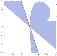
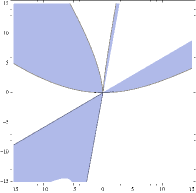
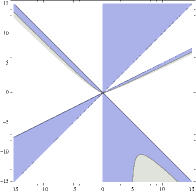
Figure 11: Central charge of dP₂ on $\Sigma=\mathbb{T}^{2}$ for different values of the integer fluxes. We plot the regions of fluxes $b_{i}$ in which the central charge assumes a positive value. In the first case we have fixed $b_{1}=x$, $b_{2}=y$ and $b_{3}=b_{4}=0$. In the second case we have fixed $b_{3}=x$ and $b_{4}=y$ and $b_{1}=b_{2}=0$. In the third case we have fixed $b_{2}=x$, $b_{3}=y$ and $b_{1}=b_{4}=0$.

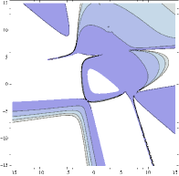
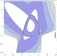
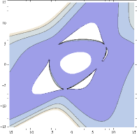
Figure 12: Central charge of dP₂ on $\Sigma=\mathbb{S}^{2}$ for different values of the integer fluxes. We plot the regions of fluxes $b_{i}$ in which the central charge assumes a positive value. In the first case we have fixed $b_{1}=x$, $b_{2}=y$ and $b_{3}=b_{4}=0$. In the second case we have fixed $b_{3}=x$ and $b_{4}=y$ and $b_{1}=b_{2}=0$. In the third case we have fixed $b_{2}=x$, $b_{3}=y$ and $b_{1}=b_{4}=0$.

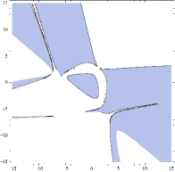
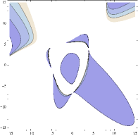
Figure 13: Central charge of dP₂ on $\Sigma=\mathbb{H}^{2}$ for different values of the integer fluxes. We plot the regions of fluxes $b_{i}$ in which the central charge assumes a positive value. In the first case we have fixed $b_{1}=x$, $b_{2}=y$ and $b_{3}=b_{4}=0$. In the second case we have fixed $b_{3}=x$ and $b_{4}=y$ and $b_{1}=b_{2}=0$. In the third case we have fixed $b_{2}=x$, $b_{3}=y$ and $b_{1}=b_{4}=0$.

dP₃

We now consider the quiver gauge theory living on a stack of D3 branes probing the tip of the complex cone over dP₃. The global currents of the model are a UV R-current $R_{0}$, two flavor currents $F_{1,2}$ and three non-anomalous baryonic currents $B_{1,2,3}$.

We can identify the baryonic currents as follows. The model has six gauge groups and classically there are six conserved baryonic currents. Two of them are anomalous and one is redundant. One is left with three non–anomalous baryonic symmetries. We can choose the charges of the fields with respect of the global symmetries as

$$\begin{array}[]{c|cccccccccccc}&X_{12}&X_{13}&X_{23}&X_{24}&X_{34}&X_{35}&X_{45}&X_{46}&X_{56}&X_{51}&X_{61}&X_{62}\\ \hline\cr R_{0}&2&0&0&0&0&2&0&2&0&0&0&0\\ F_{1}&-1&1&0&-1&1&-2&1&-1&0&1&-1&2\\ F_{2}&3&0&-1&-4&1&0&1&2&-1&0&-3&2\\ B_{1}&2&1&-1&-1&0&0&0&1&1&-1&-2&0\\ B_{2}&1&0&-1&-1&0&1&1&0&-1&-1&0&1\\ B_{3}&-1&-1&0&1&1&0&-1&-1&0&1&1&0\\ \end{array},$$

Any linear combination

$$R_{\operatorname{trial}} = R_{0}+\epsilon_{1}T_{F_{1}}+\epsilon_{2}T_{F_{2}}+\eta_{1}T_{B_{1}}+\eta_{2}T_{B_{2}}+\eta_{3}T_{B_{3}}$$ (73)

is still an R-current. The mixing coefficients in (73) are fixed by maximizing the central charge, and in this case we find

$$\epsilon_{1}=\frac{2}{3},\quad\epsilon_{2}=-\frac{1}{3},\quad\eta_{i}=0$$ (74)

Again we chose a parameterization such that at the superconformal fixed point the contribution of the baryonic symmetries vanishes.

The partial topological twist on $\Sigma$ is performed along the generator

$$T=\kappa T_{R}+b_{1}T_{F_{1}}+b_{2}T_{F_{2}}+b_{3}T_{B_{1}}+b_{4}T_{B_{2}}+b_{5}T_{B_{3}}$$ (75)

The central charge $c_{r}$ is obtained from (2.2). The final expressions are too complicated and we do not learn much in writing them explicitly. The main point is that, as in the case of dP₂, the mixing parameters are non–vanishing (see appendix A for some examples) for generic choices of the curvature and the $b_{\bf I}$ fluxes. This signals the fact that the baryonic symmetries mix with the 2d exact R–current.

We conclude by showing in Figure 14, 15 and 16 the central charge for different values of the discrete fluxes for dP₂ compactified on $\Sigma=\mathbb{T}^{2}$, $\Sigma=\mathbb{S}^{2}$ and $\Sigma=\mathbb{H}^{2}$, respectively.

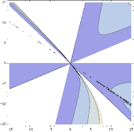
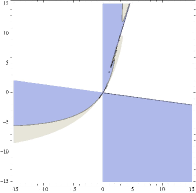
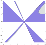
$b_{1}=x$, $b_{2}=y$ $b_{3}=b_{4}=b_{5}=0$	$b_{3}=x$, $b_{4}=y$ $b_{1}=b_{2}=b_{5}=0$	$b_{2}=x$, $b_{3}=y$ $b_{1}=b_{4}=b_{5}=0$

Figure 14: Central charge of dP₃ on $\Sigma=\mathbb{T}^{2}$ for different values of the integer fluxes. We plot the regions of fluxes $b_{i}$ in which the central charge assumes a positive value. The variable $x$ is plotted on the horizontal axis while $y$ on the vertical one.

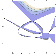
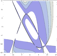
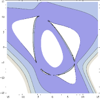
Figure 15: Central charge of dP₃ on $\Sigma=\mathbb{S}^{2}$ for different values of the integer fluxes. We plot the regions of fluxes $b_{i}$ in which the central charge assumes a positive value. In the first case we have fixed $b_{1}=x$, $b_{2}=y$ and $b_{3}=b_{4}=b_{5}0$. In the second case we have fixed $b_{3}=x$ and $b_{4}=y$ and $b_{1}=b_{2}=b_{5}0$. In the third case we have fixed $b_{2}=x$, $b_{3}=y$ and $b_{1}=b_{4}=b_{5}=0$.

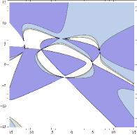
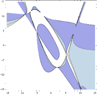
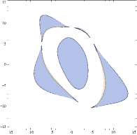
Figure 16: Central charge of dP₃ on $\Sigma=\mathbb{H}^{2}$ for different values of the integer fluxes. We plot the regions of fluxes $b_{i}$ in which the central charge assumes a positive value. In the first case we have fixed $b_{1}=x$, $b_{2}=y$ and $b_{3}=b_{4}=b_{5}0$. In the second case we have fixed $b_{3}=x$ and $b_{4}=y$ and $b_{1}=b_{2}=b_{5}0$. In the third case we have fixed $b_{2}=x$, $b_{3}=y$ and $b_{1}=b_{4}=b_{5}=0$.

$L^{pqp}$ theories

As a last example we consider models with a higher number of baryonic symmetries, i.e. $L^{pqp}$ models Benvenuti:2005ja ; Butti:2005sw ; Franco:2005sm . In order to have a comprehensive discussion we pick up a particular (Seiberg dual) phase, that can be easily visualized by the description of the system in terms of D4 and NS branes in type IIA string theory (the other phases are obtained by exchanging the NS branes). We consider a stack of N D4 branes extended along $x_{0123}$ and wrapping the compact direction $x_{6}$. Then we consider two sets of $p$ NS and $q$ NS’ branes. The NS branes are extended along $x_{012345}$ and the NS’ along $x_{012389}$. We order the NS branes and then the NS’ branes clockwise along $x_{6}$.

Each gauge group is associated to a segment of N D4 branes on $x_{6}$, suspended between two consecutive NS branes. The resulting field theory is a $U(N)$ necklace quiver gauge theory with different types of nodes. By counting clockwise on $x_{6}$ we have

• a set of $p-1$ nodes with an adjoint of type $C$;

• a node without any adjoint ;

• a set of $q-1$ nodes with an adjoint of type $\tilde{C}$;

• a node without any adjoint.

The $2p$ bifundamental matter fields crossing a NS brane are of type $A$ or $B$ depending on their orientation and the second set of $2q$ bifundamental fields, crossing a NS’ brane, are of type $\tilde{A}$ and $\tilde{B}$. We can visualize the situation in the quiver of Figure 17 for the case or $p=2$ and $q=4$.

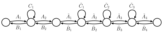
Figure 17: Quiver of the $L^{242}$ model. The first and the last node are identified.

These theories are characterized by one R–current, two flavor currents and $p+q$ baryonic currents Benvenuti:2005ja ; Butti:2005sw ; Franco:2005sm . One baryonic current is redundant, being the quiver necklace. The vector–like nature of the field content ensures that the other $p+q-1$ currents are all conserved at quantum level. The charge assignment of flavor and R-currents is summarized in the following table

$$\begin{array}[]{ccccc}\operatorname{field}&\operatorname{mult}&F_{1}&F_{2}&R_{0}\\ \hline\cr A&p&0&1&0\\ B&p&-1&0&0\\ \tilde{A}&q&1&0&1\\ \tilde{B}&q&0&-1&1\\ C&p-1&1&-1&2\\ \tilde{C}&q-1&-1&1&0\end{array}$$ (76)

The baryonic currents are associated to the $U(1)_{i}\subset U(N)_{i}$ gauge factors and the charges are read from the representation of each field under the gauge groups. Fundamental fields of $SU(N)_{i}$ have charge $+1$ and anti-fundamental fields of $SU(N)_{i}$ have charge $-1$ under the baryonic $U(1)_{i}$.

The 4d R-charge mixes with the global symmetries through the combination

$$R=R_{0}+\epsilon_{1}F_{1}+\epsilon_{2}T_{F_{2}}+\sum_{i=1}^{p+q-1}\eta_{i}T_{B_{i}}$$ (77)

with mixing parameters

$$\epsilon_{1}=\frac{\sqrt{p^{2}-pq+q^{2}}-2p+q}{3(p-q)},\quad\epsilon_{2}=\frac{p}{\sqrt{p^{2}-pq+q^{2}}+2p-q},\quad\eta_{i}=0$$ (78)

determined by the $a$–maximization.

When the theory is partially topologically twisted on $\Sigma$ along the generator

$$T=\kappa T_{R}+b_{1}T_{F_{1}}+b_{2}T_{F_{2}}+\sum_{i=1}^{p+q-1}b_{i+2}B_{i}$$ (79)

the central charge $c_{r}$ is obtained from (2.2) and extremized respect to the $\epsilon_{I}$ parameters. The final formulas are too involved and we do not report them here. The mixing parameters are non-vanishing for generic choices of the curvature and of the fluxes $b_{\bf I}$. This signals the fact that the baryonic symmetries mix with the 2d exact R-current.

In the following we show some numerical result for the 2d central charge for the $L^{222}$ and the $L^{131}$ gauge theories. In both cases there are four gauge groups and three non–anomalous baryonic symmetries. In both case we observe that the baryonic symmetries mix for generic values of the with the R–current at the 2d fixed point.

In Figure 18 and 19 we represent the central charge for different values of the discrete fluxes for $L^{222}$ compactified on $\Sigma=\mathbb{H}^{2}$ and $\Sigma=\mathbb{S}^{2}$, respectively.

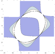
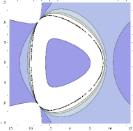
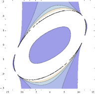
Figure 18: Central charge of L²²² on $\Sigma=\mathbb{H}^{2}$ for different values of the integer fluxes. We plot the regions of fluxes $b_{i}$ in which the central charge assumes a positive value. In the first case we have fixed $b_{1}=x$, $b_{2}=y$ and $b_{3}=b_{4}=b_{5}=0$. In the second case we have fixed $b_{3}=x$ and $b_{4}=y$ and $b_{1}=b_{2}=b_{5}=0$. In the third case we have fixed $b_{2}=x$, $b_{4}=y$ and $b_{1}=b_{3}=b_{5}=0$.

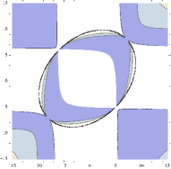
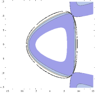
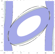
Figure 19: Central charge of L²²² on $\Sigma=\mathbb{S}^{2}$ for different values of the integer fluxes. We plot the regions of fluxes $b_{i}$ in which the central charge assumes a positive value. In the first case we have fixed $b_{1}=x$, $b_{2}=y$ and $b_{3}=b_{4}=b_{5}=0$. In the second case we have fixed $b_{3}=x$ and $b_{4}=y$ and $b_{1}=b_{2}=b_{5}=0$. In the third case we have fixed $b_{2}=x$, $b_{4}=y$ and $b_{1}=b_{3}=b_{5}=0$.

In the case of the torus reduction ($\kappa=0$) the formulae are simpler and we can provide the analytical expression for $c_{r}$ extremized with respect to the mixing parameters, in terms of the $b_{i}$ fluxes

$$\begin{array}[]{rcl}\tiny c_{r}^{L^{222},T^{2}}={\frac{6(b_{3}^{2}+b_{1}b_{3}+b_{2}b_{3}-2b_{4}b_{3}+2b_{4}^{2}+b_{5}^{2}+2b_{1}b_{2}-(b_{1}+b_{2}+2b_{4})b_{5})(b_{3}^{2}+b_{5}^{2}+b_{2}(b_{5}-b_{3})+b_{1}(2b_{2}-b_{3}+b_{5}))}{(b_{1}-b_{2})(b_{4}^{2}-b_{3}b_{4}+b_{1}b_{3}+b_{2}b_{3}-(b_{1}+b_{2}+b_{4})b_{5})}}\end{array}$$ (80)

The parameters $\epsilon_{i}^{*}$ are generically non vanishing for both the flavor and the baryonic global symmetries.

In Figure 20 and 21 we represent the central charge for different values of the discrete fluxes for $L^{131}$ compactified on $\Sigma=\mathbb{H}^{2}$ and $\Sigma=\mathbb{S}^{2}$ respectively.

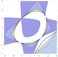
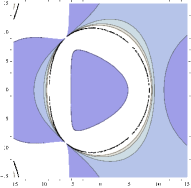
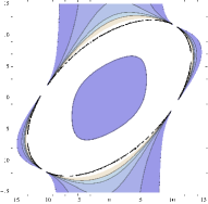
Figure 20: Central charge of L¹³¹ on $\Sigma=\mathbb{H}^{2}$ for different values of the integer fluxes. We plot the regions of fluxes $b_{i}$ in which the central charge assumes a positive value. In the first case we have fixed $b_{1}=x$, $b_{2}=y$ and $b_{3}=b_{4}=b_{5}=0$. In the second case we have fixed $b_{3}=x$ and $b_{4}=y$ and $b_{1}=b_{2}=b_{5}=0$. In the third case we have fixed $b_{2}=x$, $b_{4}=y$ and $b_{1}=b_{3}=b_{5}=0$.

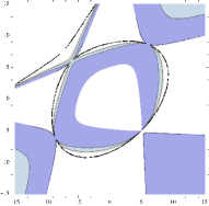
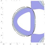
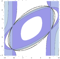
Figure 21: Central charge of L¹³¹ on $\Sigma=\mathbb{S}^{2}$ for different values of the integer fluxes. We plot the regions of fluxes $b_{i}$ in which the central charge assumes a positive value. In the first case we have fixed $b_{1}=x$, $b_{2}=y$ and $b_{3}=b_{4}=b_{5}=0$. In the second case we have fixed $b_{3}=x$ and $b_{4}=y$ and $b_{1}=b_{2}=b_{5}=0$. In the third case we have fixed $b_{2}=x$, $b_{4}=y$ and $b_{1}=b_{3}=b_{5}=0$.

In the case of the torus reduction ($\kappa=0$) the formulae are simpler and we can provide the analytical expression for $c_{r}$ extremized with respect to the mixing parameters, in terms of the $b_{i}$ fluxes

$$\begin{array}[]{rcl}\tiny c_{r}^{L^{131},T^{2}}&=&6\left(\frac{(b_{1}^{2}-3b_{2}b_{1}+b_{2}^{2}-b_{3}^{2}+(b_{1}+b_{2})b_{3}){}^{2}}{(b_{1}-b_{2})((b_{1}^{2}+(b_{3}-b_{2})b_{1}+b_{2}^{2}+b_{4}^{2}+b_{5}^{2}+b_{2}b_{3}-b_{3}b_{4}-b_{4}b_{5})}-\frac{b_{1}^{2}+4b_{2}b_{1}-2b_{3}b_{1}-b_{2}^{2}+2b_{3}^{2}-2b_{2}b_{3}}{b_{1}-b_{2}}\right)\end{array}$$ (81)

Also in this case we observe that the parameters $\epsilon_{i}^{*}$ are generically non vanishing for both the flavor and the baryonic global symmetries.

6 Further directions

In this paper we have studied c-extremization for 2d $\mathcal{N}=(0,2)$ SCFTs arising from the twisted compactification of 4d SCFTs on compact, constant curvature Riemann surfaces. The SCFTs under investigation consist of infinite families of quiver gauge theories holographically dual to D3 branes probing the tip of CY₃ cones over X₅ basis admitting a $U(1)^{3}$ toric action. In such cases we have been able to develop a simple geometric formulation for the 2d central charge $c_{r}$ in terms of its mixing with the global currents.

This formulation borrows many ideas and constructions developed in the 4d parent theory, in which it has been demonstrated that the conformal anomaly $a$ is proportional to the inverse of the X₅ volume. The geometric analogy with the 4d formulation that we have discussed may be helpful in understanding the possible relation between $c_{r}$ and the volume of the seven manifold Kim:2005ez ; Gauntlett:2007ts in the conjectured AdS${}_{3}\times\mathcal{M}_{7}$ correspondence (or eight manifolds in M–theory). It should be interesting to investigate this direction further.

In our analysis we have shown that the 2d central charge, expressed in terms of the mixing parameters, can be reformulated in the language of the toric geometry underlining the moduli space of the 4d theory. Nevertheless we did not give a general discussion on the extremization of this function. This point certainly deserves a separate and deep analysis. Indeed, the existence of an extremum is not guaranteed, as discussed in Benini:2012cz . The main obstructions are due to the absence of a normalizable vacuum of the 2d CFT and to the presence of accidental symmetries at the IR fixed point. The study of this problem would be simplified by the knowledge of the spectrum and the interactions of the 2d models. Progresses in such directions have been made in Almuhairi:2011ws ; Kutasov:2013ffl ; Gadde:2015wta . On the geometric side it would be interesting to see if some of the tools developed in 4d (e.g. the zonotope discussed in Kato:2006vx ) can be useful for the analysis of the extremization properties of the 2d central charge.

As a last comment we wish to mention that recently infinite families of 2d SCFTs have been obtained by exploiting the role of the toric geometry Franco:2015tna ; Franco:2015tya . These theories, denoted as brane brick models, are expected to describe the worldvolume theory of stacks of D1 branes probing the tip of toric CY₄ cones in type IIB. It has been shown that in such cases the toric geometry can be used to obtain the elliptic genus Franco:2017cjj . It would be interesting to further explore the role of toric geometry in these 2d SCFTs and look for possible connections, if any, with our results.

Appendix A Mixing parameters for dP₂ and dP₃

In this appendix we report the value of the mixing parameters for some choices of fluxes for the dP₂ and the dP₃ models studied in the body of the paper. The general results are pretty involved, so we restrict to some simple choices of fluxes $b_{\mathbf{I}}$.

In the dP₂ case we just show the $\kappa=0$ case and one non vanishing flux each time. By following the notations of section 5 we refer to $\epsilon$ as the mixing parameters of the flavor symmetries and to $\eta$ as the mixing parameters of the baryonic symmetries. We have the following cases

• $b_{1}\neq 0$

  $$\epsilon_{1} = \phantom{+}\frac{7b_{1}^{4}+85b_{1}^{3}-1800b_{1}^{2}-4500b_{1}+60000}{13b_{1}^{4}+310b_{1}^{3}-6375b_{1}^{2}+7000b_{1}+100000}$$

  $$\epsilon_{2} = \phantom{+}\frac{11b_{1}^{4}+110b_{1}^{3}-225b_{1}^{2}-3250b_{1}-10000}{13b_{1}^{4}+310b_{1}^{3}-6375b_{1}^{2}+7000b_{1}+100000}$$

  $$\eta_{1} = -\frac{3b_{1}^{4}-20b_{1}^{3}-525b_{1}^{2}+2000b_{1}}{13b_{1}^{4}+310b_{1}^{3}-6375b_{1}^{2}+7000b_{1}+100000}$$

  $$\eta_{2} = -\frac{18b_{1}^{4}-10b_{1}^{3}-600b_{1}^{2}-500b_{1}}{13b_{1}^{4}+310b_{1}^{3}-6375b_{1}^{2}+7000b_{1}+100000}$$ (82)

• $b_{2}\neq 0$

  $$\epsilon_{1} = -\frac{8b_{2}^{4}-270b_{2}^{3}+2600b_{2}^{2}-1250b_{2}-45000}{180b_{2}^{3}-3825b_{2}^{2}+4500b_{2}+75000}$$

  $$\epsilon_{2} = -\frac{8b_{2}^{3}-175b_{2}^{2}+525b_{2}+500}{12b_{2}^{3}-255b_{2}^{2}+300b_{2}+5000}$$

  $$\eta_{1} = -\frac{4b_{2}^{4}-135b_{2}^{3}+850b_{2}^{2}-1000b_{2}}{180b_{2}^{3}-3825b_{2}^{2}+4500b_{2}+75000}$$

  $$\eta_{2} = -\frac{8b_{2}^{4}-270b_{2}^{3}+2000b_{2}^{2}+250b_{2}}{180b_{2}^{3}-3825b_{2}^{2}+4500b_{2}+75000}$$ (83)

• $b_{3}\neq 0$

  $$\epsilon_{1}=\frac{3}{5},\quad\epsilon_{2}=-\frac{1}{10},\quad\eta_{1}=-\frac{b_{3}}{10},\quad\eta_{2}=0$$ (84)

• $b_{4}\neq 0$

  $$\epsilon_{1} = \phantom{+}\frac{95b_{4}^{3}-900b_{4}^{2}+45000}{3b_{4}^{4}-1950b_{4}^{2}+1500b_{4}+75000}$$

  $$\epsilon_{2} = -\frac{4b_{4}^{4}+5b_{4}^{3}-1000b_{4}^{2}+1000b_{4}+5000}{2b_{4}^{4}-1300b_{4}^{2}+1000b_{4}+50000}$$

  $$\eta_{2} = -\frac{12b_{4}^{4}+175b_{4}^{3}+750b_{4}^{2}-1500b_{4}}{6b_{4}^{4}-3900b_{4}^{2}+3000b_{4}+150000}$$

  $$\eta_{2} = \phantom{+}\frac{6b_{4}^{4}+80b_{4}^{3}-1800b_{4}^{2}-6000b_{4}}{3b_{4}^{4}-1950b_{4}^{2}+1500b_{4}+75000}$$ (85)

It is interesting to observe that in each case all the mixing parameters are non–vanishing, showing the general fact that the baryonic symmetries have a non trivial mix with the R–current in 2d.

In the dP₃ case we consider the case of generic $\kappa$ ($\kappa^{2}=1$) and again we fix only one non vanishing flux for each case. We have the following cases

• $b_{1}\neq 0$

  $$\epsilon_{1} = \phantom{+}\frac{16979b_{1}-6982b_{1}^{2}\kappa-740b_{1}^{3}+171360\kappa}{52998b_{1}-4416b_{1}^{2}\kappa-1104b_{1}^{3}+235116\kappa}$$

  $$\epsilon_{2} = -\frac{8165b_{1}-844b_{1}^{2}\kappa-188b_{1}^{3}+42840\kappa}{26499b_{1}-2208b_{1}^{2}\kappa-552b_{1}^{3}+117558\kappa}$$

  $$\eta_{1} = -\frac{105b_{1}+16b_{1}^{2}\kappa+4b_{1}^{3}+630\kappa}{8833b_{1}-736b_{1}^{2}\kappa-184b_{1}^{3}+39186\kappa}$$

  $$\eta_{2} = \phantom{+}\frac{920b_{1}-1948b_{1}^{2}\kappa-464b_{1}^{3}-630\kappa}{26499b_{1}-2208b_{1}^{2}\kappa-552b_{1}^{3}+117558\kappa}$$

  $$\eta_{3} = \phantom{+}\frac{605b_{1}-1996b_{1}^{2}\kappa-476b_{1}^{3}-2520\kappa}{52998b_{1}-4416b_{1}^{2}\kappa-1104b_{1}^{3}+235116\kappa}$$ (86)

• $$\epsilon_{1} = -\frac{4\left(5640b_{2}-41298b_{2}^{2}\kappa+840b_{2}^{3}+737b_{2}^{4}\kappa-52b_{2}^{5}+514080\kappa\right)}{3\left(43536b_{2}+116452b_{2}^{2}\kappa-1952b_{2}^{3}-2053b_{2}^{4}\kappa+104b_{2}^{5}-940464\kappa\right)}$$

  $$\epsilon_{2} = \phantom{+}\frac{199452b_{2}-177054b_{2}^{2}\kappa+1767b_{2}^{3}+4138b_{2}^{4}\kappa-338b_{2}^{5}+1028160\kappa}{130608b_{2}+349356b_{2}^{2}\kappa-5856b_{2}^{3}-6159b_{2}^{4}\kappa+312b_{2}^{5}-2821392\kappa}$$

  $$\eta_{1} = \phantom{+}\frac{51420b_{2}+15446b_{2}^{2}\kappa-8649b_{2}^{3}-1289b_{2}^{4}\kappa+156b_{2}^{5}+15120\kappa}{43536b_{2}+116452b_{2}^{2}\kappa-1952b_{2}^{3}-2053b_{2}^{4}\kappa+104b_{2}^{5}+940464\kappa}$$

  $$\eta_{2} = \phantom{+}\frac{960b_{2}+66888b_{2}^{2}\kappa-39906b_{2}^{3}-4054b_{2}^{4}\kappa+728b_{2}^{5}+15120\kappa}{130608b_{2}+349356b_{2}^{2}\kappa-5856b_{2}^{3}-6159b_{2}^{4}\kappa+312b_{2}^{5}-2821392\kappa}$$

  $$\eta_{3} = \phantom{+}\frac{79500b_{2}+63198b_{2}^{2}\kappa-30447b_{2}^{3}-4835b_{2}^{4}\kappa+364b_{2}^{5}+30240\kappa}{3\left(43536b_{2}+116452b_{2}^{2}\kappa-1952b_{2}^{3}-2053b_{2}^{4}\kappa+104b_{2}^{5}-940464\kappa\right)}$$

• $$\epsilon_{1} = -\frac{15660b_{3}\kappa-19524b_{3}^{2}+1857b_{3}^{3}\kappa-41b_{3}^{4}+2056320}{3\left(25344b_{3}\kappa+27384b_{3}^{2}-41b_{3}^{4}-940464\right)}$$

  $$\epsilon_{2} = \phantom{+}\frac{18180b_{3}\kappa-21588b_{3}^{2}+3729b_{3}^{3}\kappa+41b_{3}^{4}+1028160}{3\left(25344b_{3}\kappa+27384b_{3}^{2}-41b_{3}^{4}-940464\right)}$$

  $$\eta_{1} = \phantom{+}\frac{107484b_{3}\kappa-3564b_{3}^{2}-3245b_{3}^{3}\kappa+2b_{3}^{4}+15120}{25344b_{3}\kappa+27384b_{3}^{2}-41b_{3}^{4}-940464}$$

  $$\eta_{2} = -\frac{2\left(11340b_{3}\kappa+366b_{3}^{2}+1749b_{3}^{3}\kappa-164b_{3}^{4}-7560\right)}{3\left(25344b_{3}\kappa+27384b_{3}^{2}-41b_{3}^{4}-940464\right)}$$

  $$\eta_{3} = \phantom{+}\frac{4\left(21690b_{3}\kappa+246b_{3}^{2}-357b_{3}^{3}\kappa+44b_{3}^{4}+7560\right)}{3\left(25344b_{3}\kappa+27384b_{3}^{2}-41b_{3}^{4}-940464\right)}$$ (88)

• $$\epsilon_{1} = -\frac{3450b_{4}\kappa-15095b_{4}^{2}+1028160}{27288b_{4}\kappa+25014b_{4}^{2}-1410696}$$

  $$\epsilon_{2} = -\frac{3450b_{4}\kappa+7645b_{4}^{2}-514080}{27288b_{4}\kappa+25014b_{4}^{2}-1410696}$$

  $$\eta_{1}3 = \phantom{+}\frac{3330b_{4}\kappa-65b_{4}^{2}+7560}{9096b_{4}\kappa+8338b_{4}^{2}-470232}$$

  $$\eta_{2} = \phantom{+}\frac{62178b_{4}-1894b_{4}^{2}\kappa-1137b_{4}^{3}+3780\kappa}{13644b_{4}\kappa^{2}+12507b_{4}^{2}\kappa-705348\kappa}$$

  $$\eta_{3} = \phantom{+}\frac{7410b_{4}\kappa+565b_{4}^{2}+7560}{13644b_{4}\kappa+12507b_{4}^{2}-705348}$$ (89)

• $$\epsilon_{1} = -\frac{3450b_{5}\kappa+15095b_{5}^{2}-1028160}{27288b_{5}\kappa-25014b_{5}^{2}+1410696}$$

  $$\epsilon_{2} = \phantom{+}\frac{3450b_{5}\kappa+3725b_{5}^{2}-257040}{13644b_{5}\kappa-12507b_{5}^{2}+705348}$$

  $$\eta_{1} = -\frac{60b_{5}\kappa-65b_{5}^{2}+3780}{4548b_{5}\kappa-4169b_{5}^{2}+235116}$$

  $$\eta_{2} = -\frac{7590b_{5}\kappa-760b_{5}^{2}+3780}{13644b_{5}\kappa-12507b_{5}^{2}+705348}$$

  $$\eta_{3} = \phantom{+}\frac{3593b_{5}^{2}\kappa-2274b_{5}^{3}+114366b_{5}+15120\kappa}{25014b_{5}^{2}\kappa-27288b_{5}-1410696\kappa}$$ (90)

Again we observe that the mixing parameters $\eta_{i}$, that were vanishing in the 4d case, are non zero in two dimensions.

References

- (1) J. L. Cardy, Is There a c Theorem in Four-Dimensions?, Phys. Lett. B215 (1988) 749–752.
- (2) Z. Komargodski and A. Schwimmer, On Renormalization Group Flows in Four Dimensions, JHEP 12 (2011) 099, [arXiv:1107.3987].
- (3) D. Anselmi, D. Z. Freedman, M. T. Grisaru, and A. A. Johansen, Nonperturbative formulas for central functions of supersymmetric gauge theories, Nucl. Phys. B526 (1998) 543–571, [hep-th/9708042].
- (4) K. A. Intriligator and B. Wecht, The Exact superconformal R symmetry maximizes a, Nucl. Phys. B667 (2003) 183–200, [hep-th/0304128].
- (5) A. B. Zamolodchikov, Irreversibility of the Flux of the Renormalization Group in a 2D Field Theory, JETP Lett. 43 (1986) 730–732. [Pisma Zh. Eksp. Teor. Fiz.43,565(1986)].
- (6) F. Benini and N. Bobev, Exact two-dimensional superconformal R-symmetry and c-extremization, Phys. Rev. Lett. 110 (2013), no. 6 061601, [arXiv:1211.4030].
- (7) E. Witten, Topological Sigma Models, Commun. Math. Phys. 118 (1988) 411.
- (8) M. Bershadsky, A. Johansen, V. Sadov, and C. Vafa, Topological reduction of 4-d SYM to 2-d sigma models, Nucl. Phys. B448 (1995) 166–186, [hep-th/9501096].
- (9) G. Festuccia and N. Seiberg, Rigid Supersymmetric Theories in Curved Superspace, JHEP 06 (2011) 114, [arXiv:1105.0689].
- (10) D. Kutasov and J. Lin, (0,2) Dynamics From Four Dimensions, Phys. Rev. D89 (2014), no. 8 085025, [arXiv:1310.6032].
- (11) F. Benini, N. Bobev, and P. M. Crichigno, Two-dimensional SCFTs from D3-branes, JHEP 07 (2016) 020, [arXiv:1511.09462].
- (12) J. M. Maldacena and C. Nunez, Supergravity description of field theories on curved manifolds and a no go theorem, Int. J. Mod. Phys. A16 (2001) 822–855, [hep-th/0007018]. [,182(2000)].
- (13) N. Kim, AdS(3) solutions of IIB supergravity from D3-branes, JHEP 01 (2006) 094, [hep-th/0511029].
- (14) J. P. Gauntlett and N. Kim, Geometries with Killing Spinors and Supersymmetric AdS Solutions, Commun. Math. Phys. 284 (2008) 897–918, [arXiv:0710.2590].
- (15) S. Benvenuti, S. Franco, A. Hanany, D. Martelli, and J. Sparks, An Infinite family of superconformal quiver gauge theories with Sasaki-Einstein duals, JHEP 06 (2005) 064, [hep-th/0411264].
- (16) K. D. Kennaway, Brane Tilings, Int. J. Mod. Phys. A22 (2007) 2977–3038, [arXiv:0706.1660].
- (17) S. Franco, Y.-H. He, C. Sun, and Y. Xiao, A Comprehensive Survey of Brane Tilings, arXiv:1702.03958.
- (18) D. Martelli, J. Sparks, and S.-T. Yau, The Geometric dual of a-maximisation for Toric Sasaki-Einstein manifolds, Commun. Math. Phys. 268 (2006) 39–65, [hep-th/0503183].
- (19) A. Butti and A. Zaffaroni, R-charges from toric diagrams and the equivalence of a-maximization and Z-minimization, JHEP 11 (2005) 019, [hep-th/0506232].
- (20) B. Feng, A. Hanany, and Y.-H. He, D-brane gauge theories from toric singularities and toric duality, Nucl. Phys. B595 (2001) 165–200, [hep-th/0003085].
- (21) M. Bertolini, F. Bigazzi, and A. L. Cotrone, New checks and subtleties for AdS/CFT and a-maximization, JHEP 12 (2004) 024, [hep-th/0411249].
- (22) S. S. Gubser, Einstein manifolds and conformal field theories, Phys. Rev. D59 (1999) 025006, [hep-th/9807164].
- (23) S. S. Gubser and I. R. Klebanov, Baryons and domain walls in an N=1 superconformal gauge theory, Phys. Rev. D58 (1998) 125025, [hep-th/9808075].
- (24) D. Martelli, J. Sparks, and S.-T. Yau, Sasaki-Einstein manifolds and volume minimisation, Commun. Math. Phys. 280 (2008) 611–673, [hep-th/0603021].
- (25) Y. Tachikawa, Five-dimensional supergravity dual of a-maximization, Nucl. Phys. B733 (2006) 188–203, [hep-th/0507057].
- (26) A. Butti and A. Zaffaroni, From toric geometry to quiver gauge theory: The Equivalence of a-maximization and Z-minimization, Fortsch. Phys. 54 (2006) 309–316, [hep-th/0512240].
- (27) A. Butti, A. Zaffaroni, and D. Forcella, Deformations of conformal theories and non-toric quiver gauge theories, JHEP 02 (2007) 081, [hep-th/0607147].
- (28) S. Benvenuti, L. A. Pando Zayas, and Y. Tachikawa, Triangle anomalies from Einstein manifolds, Adv. Theor. Math. Phys. 10 (2006), no. 3 395–432, [hep-th/0601054].
- (29) S. Lee and S.-J. Rey, Comments on anomalies and charges of toric-quiver duals, JHEP 03 (2006) 068, [hep-th/0601223].
- (30) A. Kato, Zonotopes and four-dimensional superconformal field theories, JHEP 06 (2007) 037, [hep-th/0610266].
- (31) D. R. Gulotta, Properly ordered dimers, R-charges, and an efficient inverse algorithm, JHEP 10 (2008) 014, [arXiv:0807.3012].
- (32) R. Eager, Equivalence of A-Maximization and Volume Minimization, JHEP 01 (2014) 089, [arXiv:1011.1809].
- (33) B. Feng, Y.-H. He, K. D. Kennaway, and C. Vafa, Dimer models from mirror symmetry and quivering amoebae, Adv. Theor. Math. Phys. 12 (2008), no. 3 489–545, [hep-th/0511287].
- (34) A. Hanany and D. Vegh, Quivers, tilings, branes and rhombi, JHEP 10 (2007) 029, [hep-th/0511063].
- (35) S. Franco, A. Hanany, D. Martelli, J. Sparks, D. Vegh, and B. Wecht, Gauge theories from toric geometry and brane tilings, JHEP 01 (2006) 128, [hep-th/0505211].
- (36) S. M. Hosseini, A. Nedelin, and A. Zaffaroni, The Cardy limit of the topologically twisted index and black strings in AdS5, arXiv:1611.09374.
- (37) A. Amariti, L. Cassia, and S. Penati, Surveying 4d SCFTs twisted on Riemann surfaces, arXiv:1703.08201.
- (38) F. Benini and N. Bobev, Two-dimensional SCFTs from wrapped branes and c-extremization, JHEP 06 (2013) 005, [arXiv:1302.4451].
- (39) J. D. Brown and M. Henneaux, Central Charges in the Canonical Realization of Asymptotic Symmetries: An Example from Three-Dimensional Gravity, Commun. Math. Phys. 104 (1986) 207–226.
- (40) P. Karndumri and E. O Colgain, Supergravity dual of -extremization, Phys. Rev. D87 (2013), no. 10 101902, [arXiv:1302.6532].
- (41) A. Amariti and C. Toldo, Betti multiplets, flows across dimensions and c-extremization, arXiv:1610.08858.
- (42) S. Benvenuti and M. Kruczenski, From Sasaki-Einstein spaces to quivers via BPS geodesics: L**p,q|r, JHEP 04 (2006) 033, [hep-th/0505206].
- (43) A. Butti, D. Forcella, and A. Zaffaroni, The Dual superconformal theory for L**pqr manifolds, JHEP 09 (2005) 018, [hep-th/0505220].
- (44) A. Hanany, P. Kazakopoulos, and B. Wecht, A New infinite class of quiver gauge theories, JHEP 08 (2005) 054, [hep-th/0503177].
- (45) A. Almuhairi and J. Polchinski, Magnetic AdS: Supersymmetry and stability, arXiv:1108.1213.
- (46) A. Gadde, S. S. Razamat, and B. Willett, On the reduction of 4d theories on , JHEP 11 (2015) 163, [arXiv:1506.08795].
- (47) S. Franco, D. Ghim, S. Lee, R.-K. Seong, and D. Yokoyama, 2d (0,2) Quiver Gauge Theories and D-Branes, JHEP 09 (2015) 072, [arXiv:1506.03818].
- (48) S. Franco, S. Lee, and R.-K. Seong, Brane Brick Models, Toric Calabi-Yau 4-Folds and 2d (0,2) Quivers, JHEP 02 (2016) 047, [arXiv:1510.01744].
- (49) S. Franco, D. Ghim, S. Lee, and R.-K. Seong, Elliptic Genera of 2d (0,2) Gauge Theories from Brane Brick Models, arXiv:1702.02948.