Investigating prescriptions for artificial resistivity in smoothed particle magnetohydrodynamics

Abstract

In numerical simulations, artificial terms are applied to the evolution equations for stability. To prove their validity, these terms are thoroughly tested in test problems where the results are well known. However, they are seldom tested in production-quality simulations at high resolution where they interact with a plethora of physical and numerical algorithms. We test three artificial resistivities in both the Orszag-Tang vortex and in a star formation simulation. From the Orszag-Tang vortex, the Price et. al. (2017) artificial resistivity is the least dissipative thus captures the density and magnetic features; in the star formation algorithm, each artificial resistivity algorithm interacts differently with the sink particle to produce various results, including gas bubbles, dense discs, and migrating sink particles. The star formation simulations suggest that it is important to rely upon physical resistivity rather than artificial resistivity for convergence.

I Introduction

When applying artificial dissipation terms to the smoothed particle magnetohydrodynamics (SPMHD) equations, one must be careful to apply enough such that the simulation is stable, but not too much such that the results become dominated by the artificial terms. Moreover, the artificial corrections should only be applied in regions where it is required (e.g. at shocks), and at the minimal amount required for accurate capturing of shocks and other discontinuities. Thus, determining how, where and when to apply the artificial dissipation terms can be a difficult undertaking.

Several switches to reduce the dissipation away from smooth flow have been derived and tested within the literature. This includes first- (e.g. [1]) and second- (e.g.[2]) order algorithms for artificial viscosity to be added to the momentum equation; artificial conductivity (e.g. [3], [4]) to be added to the energy equation; and artificial resistivity (e.g. [5],[6], [7], [8]) to be added to the induction equation for magnetic stability.

Testing the artificial terms is implicitly or explicitly done in most code/algorithm papers. This is typically done by showing how well the algorithm performs on well-defined tests (e.g. [9], [10], [11]), or on simple problems (e.g. [12], [13]). During development, these tests are useful for debugging purposes. After development, the tests are useful for benchmarking purposes, to show proof-of-concept that the algorithm works, to (cautiously) compare the algorithm to other algorithms, and to determine the limitations of the algorithm (c.f. [14]).

As expected, most codes perform poorly on test problems involving discontinuities when no artificial dissipation terms are applied; with the correct amount of artificial dissipation in the correct place, the numerical results can be made to agree well with the analytical answers (e.g. shock tubes). It should be noted that when shock tube tests are presented in the literature, they are often performed with maximal artificial corrections rather than the default values. This difference is demonstrated in figures of 29 and 30 of [8] which demonstrates the Brio & Wu shock tube [10] using both maximal and default artificial corrections. By contrast, tests involving smooth flows yield better results when no artificial dissipation is applied (e.g. the advection of a current loop [15]).

Although these artificial dissipations are rigorously tested in test problems, they are seldom tested in realistic or production-quality simulations due to their expense. However, some artefacts of the artificial algorithms may only appear at high resolution, or once all the required physics is included. Thus, coupled with the results from test problems, comparing artificial terms in production-quality simulations is required to fully understand the effects of the terms.

In this proceeding, we first discuss smoothed particle magnetohydrodynamics with the focus on magnetic fields and artificial resistivity (c.f. Section II). In Section III, we test the three resistivities using the Orszag-Tang vortex test problem and in Section IV we test the resistivities in a realistic star formation simulation. In Section V we discuss possible modifications to the resistivities, and we conclude in Section VI.

II Numerical Methods

II-A Smoothed particle magnetohydrodynamics

The continuum and numerical equations describing smoothed particle magnetohydrodynamics are readily found in the literature (e.g. [15],[16],[17],[8]). To evolve the magnetic field, the stress tensor, $S$, used to update the velocity is augmented from $S^{ij}=-P\delta^{ij}$, where $P$ is the gas pressure and $\delta^{ij}$ is the Kronecker delta, to

$$S^{ij}=-\left(P+\frac{B^{2}}{2\mu_{0}}\right)\delta^{ij}+\frac{B^{i}B^{j}}{\mu_{0}},$$ (1)

where $B$ is the magnetic field and $\mu_{0}$ is the permeability of free space. Here, $i$ and $j$ represent summation over dimensions $\{x,y,z\}$.

The evolution of the magnetic field is given by the induction equation. In the continuum limit, this is given by

$$\frac{{\rm d}B^{i}}{\text{d}t}=\left(B^{j}\nabla^{j}\right)v^{i}-B^{i}\left(\nabla^{j}v^{j}\right),\\$$ (2)

where $v$ is velocity. The discretised form for the evolution of the magnetic field on particle $a$ is

$$\frac{\text{d}B^{i}_{a}}{\text{d}t}=-\frac{1}{\Omega_{a}\rho_{a}}\sum_{b}m_{b} \left[v^{i}_{ab}B^{j}_{a}\nabla^{j}_{a}W_{ab}\left(h_{a}\right)\right.$$ (3)

$$-\left.B^{i}_{a}v^{j}_{ab}\nabla^{j}_{a}W_{ab}\left(h_{a}\right)\right],$$

where we sum over all particles $b$ within the kernel radius, $W_{ab}$ is the smoothing kernel, $\rho_{a}$ is the density, $v^{i}_{ab}\equiv v^{i}_{a}-v^{i}_{b}$, and $\Omega_{a}$ is a dimensionless correction term to account for a spatially variable smoothing length $h_{a}$ (​​[18],[19]).

Magnetic fields have the physical constraint that monopoles do not exist, i.e. $\nabla^{i}B^{i}=0$. However, this constraint is not explicitly enforced in SPMHD, thus $\nabla^{i}B^{i}\neq 0$ can be numerically obtained which can trigger the tensile instability when $\frac{1}{2}B^{2}>P$. The simplest method to correct for this is to subtract $\nabla^{i}B^{i}$ from the momentum equation viz.

$$\frac{\text{d}v^{i}_{a}}{\text{d}t}\rightarrow\frac{\text{d}v^{i}_{a}}{\text{d}t}-f_{a}B^{i}_{a}\sum_{b}m_{b} \left[\frac{B^{j}_{a}}{\Omega_{a}\rho_{a}^{2}}\nabla^{j}_{a}W_{ab}(h_{a})\right.$$

$$+ \left.\frac{B^{j}_{b}}{\Omega_{b}\rho_{b}^{2}}\nabla^{j}_{a}W_{ab}(h_{b})\right],$$ (4)

using $f_{a}=1$. Since this subtraction violates energy and momentum conservation (but only insofar as the divergence term the momentum equation is non-zero; e.g. [15], [20]), it must be treated with caution. A variable $f_{a}\in[0,\frac{1}{2}]$ has been suggested [21], however it has been shown that numerical artefacts can be produced for $f<1$, thus a more conservative suggestion is $f_{a}=1$ everywhere [20]. Since the tensile instability is only triggered for $\frac{1}{2}B^{2}>P$, we use

$$f_{a}=\left\{\begin{array}[]{l l}1;&\beta_{a}\leq 1,\\ 2-\beta_{a};&1<\beta_{a}\leq 2,\\ 0;&\beta_{a}>2,\end{array}\right.$$ (5)

where $\beta_{a}=\frac{2P_{a}}{B_{a}^{2}}$ is the plasma beta.

Finally, artificial resistivity is required to correctly capture shocks and discontinuities. Thus, the magnetic field evolution is augmented to

$$\frac{\text{d}B^{i}}{\text{d}t} = \left.\frac{\text{d}B^{i}}{\text{d}t}\right|_{\text{ideal}}+\left.\frac{\text{d}B^{i}}{\text{d}t}\right|_{\text{art}},$$ (6)

where the first term on the right-hand side is the ideal magnetohydrodynamic (MHD) term given in (2) and the second term is the artificial resistivity, which is typically represented in the form $\bm{\nabla}\times\left[\eta\left(\bm{\nabla}\times\bm{B}\right)\right]$. Three possible resistivities are described below, and all three are second-order accurate away from shocks.

II-B Price et. al. (2017) artificial resistivity: $\eta_{v\times r}$

This artificial resistivity is the default in Phantom [8] and was used in the study to investigate binary star formation [22]. The discretised form of the artificial resistivity (​​[5], [6]) is

$$\left.\frac{\text{d}B^{i}_{a}}{\text{d}t}\right|_{\text{art}}=\frac{\rho_{a}}{2}\sum_{b}m_{b}\alpha^{\text{B}}v_{\text{sig},ab}^{\text{P}}B^{i}_{ab} \left[\frac{\hat{r}^{j}_{ab}\nabla^{j}_{a}W_{ab}(h_{a})}{\Omega_{a}\rho_{a}^{2}}\right.$$ (7)

$$\left.+\frac{\hat{r}^{j}_{ab}\nabla^{j}_{a}W_{ab}(h_{b})}{\Omega_{b}\rho_{b}^{2}}\right],$$

where $\alpha^{\text{B}}\equiv 1$ is a dimensionless coefficient constant for all particles, $B^{i}_{ab}\equiv B^{i}_{a}-B^{i}_{b}$, and the signal velocity is $v_{\text{sig},ab}^{\text{P}}=|\bm{v}_{ab}\times\hat{\bm{r}}_{ab}|$.

The main point is that this artificial resistivity is second-order accurate away from shocks since the coefficient is $\eta^{\text{P}}_{a}=\alpha^{\text{B}}|\bm{v}_{ab}\times\hat{\bm{r}}_{ab}|h_{a}\propto h_{a}^{2}$. This algorithm was tested in [8] and shown to still provide sufficient dissipation at magnetic discontinuities.

II-C Tricco & Price (2013) term-averaged artificial resistivity: $\eta_{a}\!+\!\eta_{b}$

This version of artificial resistivity was included in a previous (private) version of Phantom and was used in the study to investigate isolated star formation [16]. The discretised form of the artificial resistivity is

$$\left.\frac{\text{d}B^{i}_{a}}{\text{d}t}\right|_{\text{art}}=\frac{\rho_{a}}{2}\sum_{b}m_{b}B^{i}_{ab} \left[\frac{\alpha^{\text{B}}_{a}v_{\text{sig},a}^{\text{T}}\hat{r}^{j}_{ab}\nabla^{j}_{a}W_{ab}(h_{a})}{\Omega_{a}\rho_{a}^{2}}\right.$$ (8)

$$\left.+\frac{\alpha^{\text{B}}_{b}v_{\text{sig},b}^{\text{T}}\hat{r}^{j}_{ab}\nabla^{j}_{a}W_{ab}(h_{b})}{\Omega_{b}\rho_{b}^{2}}\right],$$

where the signal velocity is $v_{\text{sig},a}^{\text{T}}=\sqrt{c_{\text{s},a}^{2}+v_{\text{A},a}^{2}}$ where $c_{\text{s},a}$ is the sound speed and $v_{\text{A},a}$ is the Alfvén velocity, and $\alpha_{a}^{\text{B}}=\min\left(h_{a}\left|\nabla\bm{B}_{a}\right|/\left|\bm{B}_{a}\right|,1\right)$. This ensures that resistivity is only strong where there are strong gradients in the magnetic field [7].

The resistivity is also second-order away from shocks, since $\eta^{\text{T}}_{a}\approx\frac{1}{2}\alpha^{\text{B}}_{a}v^{\text{T}}_{\text{sig},a}h_{a}$ and $\alpha^{\text{B}}_{a}\propto h_{a}$. Note that this coefficient can be calculated without any knowledge of the $a$’s neighbours.

II-D Tricco & Price (2013) variable-averaged resistivity: $\eta_{ab}$

The final artificial resistivity we test is similar to that used in sphNG (​​[23], [24], [25]) which was used in the study to investigate isolated star formation (​​[26],[27]). This algorithm has been incorporated into Phantom for this study. This version uses the same signal velocity, dimensionless coefficient and resistivity coefficient as in Section II-C above, but averages the terms differently; various averaging algorithms for the smoothing length have previously been studied [26] but found to be irrelevant. This artificial resistivity is given by

$$\left.\frac{\text{d}B^{i}_{a}}{\text{d}t}\right|_{\text{art}} =\frac{\rho_{a}}{2}\sum_{b}m_{b}B^{i}_{ab}\left[\frac{\left(\alpha^{\text{B}}_{a}+\alpha^{\text{B}}_{b}\right)\left(v_{\text{sig},a}^{\text{T}}+v_{\text{sig},b}^{\text{T}}\right)}{\left(\rho_{a}+\rho_{b}\right)^{2}}\right]$$ (9)

$$\times\frac{1}{2}\left[\frac{\hat{r}^{j}_{ab}\nabla^{j}_{a}W_{ab}(h_{a})}{\Omega_{a}}+\frac{\hat{r}^{j}_{ab}\nabla^{j}_{b}W_{ab}(h_{b})}{\Omega_{b}}\right].$$

III Idealised test: Orszag-Tang vortex

Standard tests for MHD include shock tubes (e.g. [10], [11]), the Orszag-Tang vortex [12], and the MHD rotor test [13]. We perform the Orszag-Tang test using the SPMHD code Phantom [8] with an adiabatic equation of state with $\gamma=5/3$.

The particles are placed on a periodic, close-packed lattice with $x,y\in[-0.5,0.5]$ and $z\in[-\frac{\sqrt{6}}{256},\frac{\sqrt{6}}{256}]$; our resolution is $512\times 590\times 12$ particles. The particles have an initial velocity and magnetic field of $[v_{x},v_{y},v_{z}]=[-v_{0}\sin(2\pi y^{\prime}),v_{0}\sin(2\pi x^{\prime}),0.01v_{0}]$ and $[B_{x},B_{y},B_{z}]=[-B_{0}\sin(2\pi y^{\prime}),B_{0}\sin(4\pi x^{\prime}),0]$, respectively, where $v_{0}=1$, $B_{0}=1/\sqrt{4\pi}$, $x^{\prime}=x-x_{\text{min}}$ and $y^{\prime}=y-y_{\text{min}}$. The initial plasma beta and Mach number are $\beta_{0}=10/3$ and $\mathcal{M}_{0}=v_{0}/c_{\text{s},0}=1$, respectively, which yield an an initial pressure and density of $P_{0}=\frac{B_{0}^{2}}{2\beta_{0}}\approx 0.133$ and $\rho_{0}=\gamma P_{0}\mathcal{M}_{0}\approx 0.221$, respectively. Physical units are irrelevant for this test.

Figure 1 shows the mid-plane gas density at $t=0.5$ (top) and $t=1$ (bottom) for the three models.

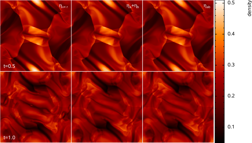
Figure 1: The mid-plane gas density for the Orszag-Tang vortex at times $t=0.5$ (top) and $t=1$ (bottom); the initial conditions are given in text. The left-hand column uses the Price et. al. (2017) artificial resistivity $\eta_{v\times r}$, the middle column uses the Tricco & Price (2013) term-averaged resistivity $\eta_{a}\!+\!\eta_{b}$, and the right-hand column uses the Tricco & Price (2013) variable-averaged resistivity $\eta_{ab}$. The results using $\eta_{a}\!+\!\eta_{b}$ or $\eta_{ab}$ yield features that are slightly more washed out than using $\eta_{v\times r}$. The results from the $\eta_{a}\!+\!\eta_{b}$ and $\eta_{ab}$ models are indistinguishable from one another.

At both times, the features are sharper when using the $\eta_{v\times r}$ resistivity; a magnetic island [28] appears near the centre of the $\eta_{v\times r}$ model at $t=1$, but not in the $\eta_{a}\!+\!\eta_{b}$ or $\eta_{ab}$ models. As previously shown in the literature, decreasing the resolution of the $\eta_{v\times r}$ model removes the magnetic island [8], thus switching to $\eta_{a}\!+\!\eta_{b}$ has a similar effect to reducing the resolution of the $\eta_{v\times r}$ model.

Figure 2 shows the evolution of the total magnetic energy.

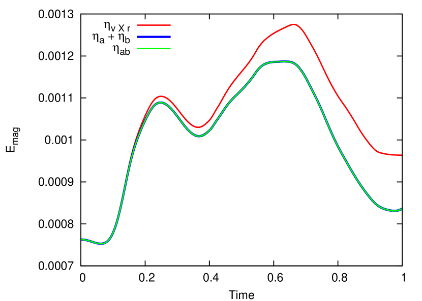
Figure 2: The evolution of the total magnetic energy for the three models presented in code units. The $\eta_{v\times r}$ model yields up to 16 per cent less dissipation (at $t\approx 0.97$) two the other two models. The total magnetic energies in $\eta_{a}\!+\!\eta_{b}$ and $\eta_{ab}$ differ by less than 0.025 per cent at any given time.

By design, the $\eta_{a}\!+\!\eta_{b}$ and $\eta_{ab}$ artificial resistivities are more dissipative, and yield a lower total magnetic energy than $\eta_{v\times r}$; at $t=0.5$ and 1, the magnetic energy is $\sim 4$ and 15 per cent lower, respectively. At all times, the magnetic energies of $\eta_{a}\!+\!\eta_{b}$ and $\eta_{ab}$ differ by less than 0.025 per cent; this is expected since there are no steep density gradients. If the magnetic energies were normalised to their initial value, then the evolution of the total magnetic energy using $\eta_{a}\!+\!\eta_{b}$ can be approximately matched by using $\eta_{v\times r}$ at a resolution of $164\times 190\times 12$.

These results suggest that the $\eta_{v\times r}$ resistivity yields better results due to its reduced dissipation, and the ability to capture magnetic and density features without needlessly increasing the resolution.

Importantly, models without any artificial resistivity are noticeably worse [8], suggesting at least a small amount of artificial resistivity is require to capture MHD discontinuities.

IV Realistic tests: Star formation

Figure 3: Face-on (left) and edge-on (right) gas column density of the isolated star formation model at selected times (in units of the free-fall time, $t_{\text{ff}}=2.4\times~{}10^{4}$ yr). The columns show the different models, and the rows show images taken at different times. The white circles represent the sink particle with the radius of the circle representing the accretion radius of the sink particle. Each frame is (300 AU)². At early times, the results are qualitatively model-independent; at late times, the $\eta_{v\times r}$ model forms bubbles, the $\eta_{a}\!+\!\eta_{b}$ model has evolved a dense disc, and the $\eta_{ab}$ model’s disc has mostly dissipated and its sink particle has levitated due to lack of momentum conservation.

For a realistic test, we simulate the formation of an isolated protostar as in e.g. [29], [30], [31], [32], [33], [34], [35], [36], [37], [26],[16],[27]. Strongly magnetised numerical simulations of star formation have historically failed to produce discs around protostars, which is contrary to what is observed. This is known as the magnetic braking catastrophe (e.g. [38], [39]). This is a result of ideal MHD (where there is no resistivity) efficiently transporting angular momentum away from the protostar, allowing the collapsing gas to be directly accreted onto the protostar rather than first entering a rotationally supported disc.

We again use Phantom for all three tests, but this time use a Barotropic equation of state, and include gravity and sink particles. To initialise the problem, we create a spherical cloud of radius $R=4\times~{}10^{16}$ cm = 0.013 pc, mass $M=1$ M_⊙, mean density of $\rho_{0}=7.43\times~{}10^{-18}$ g cm^-3 and $10^{6}$ SPH particles; we then place the sphere in a low density box of edge length $l=4R$ and a density contrast of 30:1. The cloud has an initial rotational velocity of $\Omega=1.77\times 10^{-13}$ rad s^-1, and an initial sound speed of $c_{\text{s,0}}=2.19\times 10^{4}$ cm s^-1. The entire domain is threaded with a uniform magnetic field of $B=163\mu$G which is anti-aligned with the rotation axis. The free-fall time is $t_{\text{ff}}=2.4\times~{}10^{4}$ yr, which is the characteristic timescale for this study.

To study the long term evolution of the environment after the protostar is formed, sink particles [25] are required. These are inserted when the densest gas particle reaches $\rho>\rho_{\text{crit}}=10^{-10}$g cm^-3 and given conditions at and around the sink particle candidate are met. The sink particles have an accretion radius of $h_{\text{acc}}=2$ au; any particle coming within 1 au of the sink is automatically accreted, while particles coming within 2 au are only accreted if given criteria are met. Accreted particles have their properties added to the sink and then are removed from the simulation. As per convention, there are no boundary conditions associated with the sink particles.

We ran the star formation simulation three times, only changing the artificial resistivity. Since steep gradients are expected to form near the protostar, it is worth investigating both $\eta_{a}\!+\!\eta_{b}$ and $\eta_{ab}$, despite them yielding identical results in the Orszag-Tang vortex. Figure 3 shows the face-on and edge-on gas column densities at four different times for the three models, Figure 4 shows the edge-on gas column density of the outflows at the first two times, and Figure 5 shows the azimuthally averaged gas surface density and plasma beta around the sink particle at the first two times.

Figure 4: Edge-on gas column density at two early times for the star formation simulations, as in Figure 3. Each frame is $2400\times 3600$ au so the large scale structure of the outflows can be seen; the outflows in the $\eta_{a}\!+\!\eta_{b}$ model are slower then the other two models.

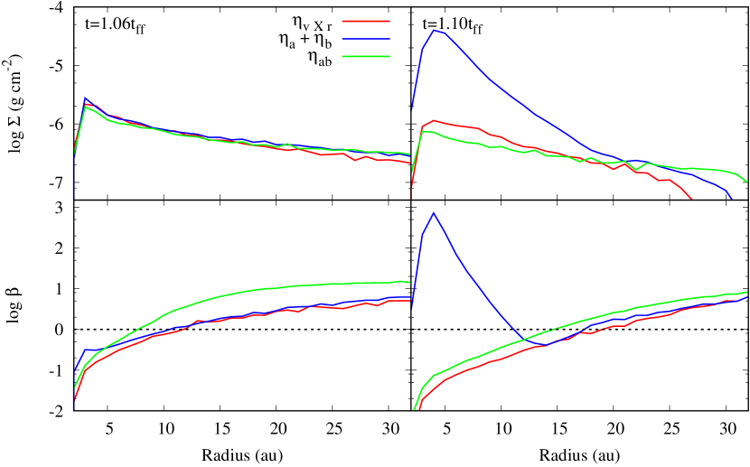
Figure 5: The azimuthally averaged gas surface density (top) and plasma beta (bottom) for the inner 32 au at two early times for the star formation simulations. The horizontal axis starts at $R=2$ au, which is the accretion radius of the sink particle. If $\beta<1$, then the gas is dominated by magnetic pressure, otherwise it is dominated by gas pressure. The results are approximately independent of resistivity model at $t=1.06t_{\text{ff}}$, however, the $\eta_{a}\!+\!\eta_{b}$ model diverges from the other two shortly thereafter.

At the early time of $t\approx 1.06t_{\text{ff}}$, the results are similar for all three models. The surface density profiles differ by at most 40 per cent, and the $\eta_{ab}$ model has a plasma beta that is 2-3 times higher than the $\eta_{v\times r}$ model. All but the inner few au are dominated by gas pressure, thus at this time, the magnetic fields are of a secondary importance over most of the domain. Thus, arguably, if the study were to end here, the specific choice of artificial resistivity would not be important.

As the models continue to evolve, they begin to diverge. By $t\approx 1.10t_{\text{ff}}$, there is a dense disc around the sink in the $\eta_{a}\!+\!\eta_{b}$ model due to its large resistivity, but not the other models; this model also has slower outflow velocities and hence the outflows have not progressed as far as in the other two models. This is consistent with previous results that showed an inverse correlation between disc size and outflow velocity [16]. At this time, the other two models have surface densities and plasma beta’s that differ by less than a factor of two; their maximum surface density is $\sim$60 times lower than in the $\eta_{a}\!+\!\eta_{b}$ model. At this time, $\eta_{v\times r}$ and $\eta_{ab}$ demonstrate the magnetic braking catastrophe whereas the $\eta_{a}\!+\!\eta_{b}$ model does not. Given that this disc is likely formed by the artificial resistivity, we must be cautious to not claim that the problem has been solved. At this stage, it is arguable that $\eta_{v\times r}$ or $\eta_{ab}$ are likely preferable algorithms since they yield similar results.

As the $\eta_{a}\!+\!\eta_{b}$ model continues to evolve, the disc slowly decreases in mass and radius, but the system remains stable. The disc slightly migrates downwards due to lack of momentum conservation; by $t\approx 1.21t_{\text{ff}}$, the sink particle has drifted d$z\approx 9.7$ au from its creation point and has a speed of $v_{\text{z}}\approx 0.03$ km s^-1. Tests have shown that the amount of migration is dependent on sink size, however, low resolution cores without sinks have also been found to migrate.

As the $\eta_{v\times r}$ and $\eta_{ab}$ models evolve, the gas density near the sink decreases, but, as in the $\eta_{a}\!+\!\eta_{b}$ model, the magnetic field continues to increase. As a result, the magnetic pressure increasingly dominates gas pressure near the sink in these two models, and stronger magnetic pressure in SPMHD results in lower momentum conservation (i.e. $\beta\ll 1$; see (II-A) and (5)). This lack of momentum conservation in the $\eta_{ab}$ model results in the sink particle migrating in the vertical direction, which drags the gas with it; azimuthal symmetry is approximately preserved. Since there is only low-density gas around the sink (as compared to $\eta_{a}\!+\!\eta_{b}$), the sink particle is capable of wandering with great speeds since there is no gas disc to exert an attractive gravitational force. By $t\approx 1.21t_{\text{ff}}$, the sink has a vertical velocity of $v_{\text{z}}\approx 0.5$ km s^-1 and moved a distance of d$z\approx 108$ au.

The sink particle in the $\eta_{v\times r}$ model has a maximum vertical wandering of $v_{\text{z}}\approx 0.009$ km s^-1; this is similar to hydrodynamical simulations that do not suffer from an intrinsic lack of momentum conservation. In this model, the momentum conservation error contributes to the gas motion, rather than the sink particle migration. Since the dominant velocity component is the radial component, the gas receives a small radial kick. Coupled with the high magnetic pressure, this ultimately causes the launching of the gas bubbles.

Figure 6 shows the evolution of the total magnetic energy.

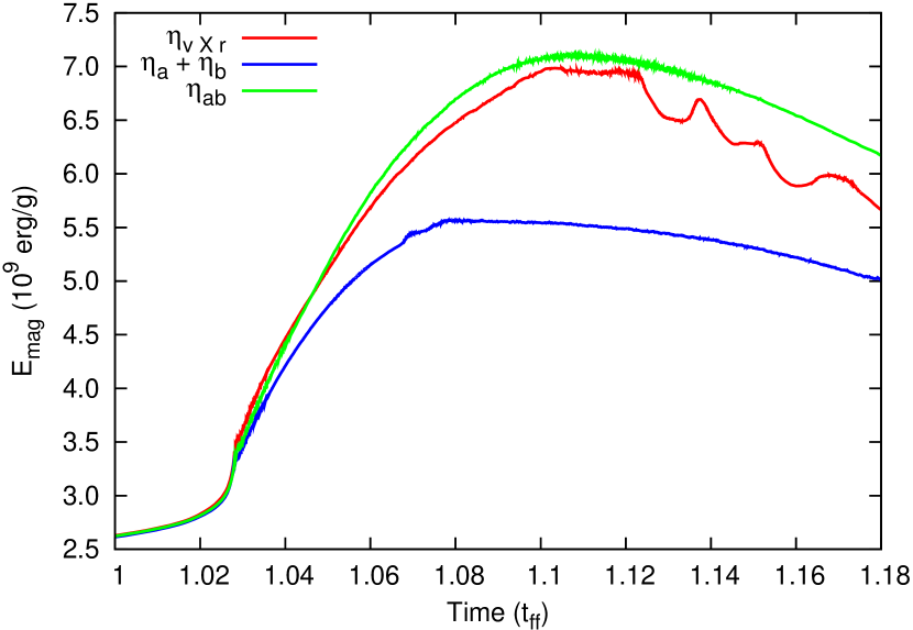
Figure 6: The evolution of the total magnetic energy for the star formation simulations. The three models begin to diverge at $t\approx 1.03t_{\text{ff}}$, which coincides with the insertion of the sink particle. The $\eta_{a}\!+\!\eta_{b}$ is the most resistive, hence the lowest total magnetic energy. The $\eta_{v\times r}$ forms the gas bubbles at $t\approx 1.12t_{\text{ff}}$, when the curve becomes less smooth.

As with the Orszag-Tang vortex, the $\eta_{a}\!+\!\eta_{b}$ model shows the most magnetic dissipation. Thus, although this model is arguably more stable than the other two, it has dissipated enough energy such that the results are at least in part being controlled by the artificial resistivity.

When we reduce the resolution to $3\times 10^{5}$ particles in the sphere, there is good agreement amongst the models at early times and their evolution diverges at late times; see Figure 7, which shows the face-on gas column density at four times for the low resolution models.

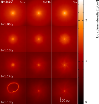
Figure 7: Face-on gas column density of the isolated star formation model at selected times as in Figure 3 except using $3\times 10^{5}$ particles in the sphere. in units of the free-fall time, $t_{\text{ff}}=2.4\times~{}10^{4}$ yr). Compared to their higher resolution counterpart, the $\eta_{v\times r}$ model is delayed in producing the gas bubbles, the $\eta_{a}\!+\!\eta_{b}$ model has a smaller disc, and the sink in the $\eta_{ab}$ model does not migrate.

At the lower resolution, the density, magnetic gradients, and the sink boundary are less resolved, thus any features that may cause the evolution to diverge in the higher resolutions models get smoothed out, thus allowing for better convergence.

As a result, the gas bubbles are launched at a later time in the lower resolution $\eta_{v\times r}$ model. The low resolution $\eta_{a}\!+\!\eta_{b}$ model has the highest surface density amongst the three low resolution runs, but this is $\sim$2 dex lower than in the higher resolution run. Prior to sink insertion, the higher resolution model has a higher density and central magnetic field simply due to the resolution. After the sink particle has been inserted, the sink grows more slowly due to the lower gas particle masses and better resolved boundaries. This leaves more gas in the sink’s environment, which ultimately forms a dense disc as the magnetic field is dissipated; the lower resolution model does not have enough gas in the vicinity of the sink to form a dense disc. In low resolution $\eta_{ab}$ model, the sink migration is minimal. Finally, since the artificial resistivity is $\eta\propto h^{2}$, there is more artificial resistivity in the lower resolution models, resulting in lower total magnetic energies.

This study is not the first time that magnetic bubbles have been discovered in MHD simulations. They have been previously found in similar 3D adaptive mesh refinement (AMR) simulations [40], although their bubbles were not confined to the mid-plane. As with this study, their magnetic bubbles were launched from the low-density gas near the sink particle, and contained strong magnetic fields. Their study was performed on a spherical-polar grid, thus similar to sink particles in SPH, there is a hole in the magnetic field around the sink particle. Thus, the same bubbles have been observed using two distinct numerical algorithms, and in both cases they originate in low-density gas near sink particles.

The long term evolution leads to a conundrum of which artificial resistivity to use: $\eta_{v\times r}$ leads to magnetic bubbles launched from near a numerical boundary, but that have been also observed in AMR simulations; $\eta_{a}\!+\!\eta_{b}$ leads to the formation of a massive disc; and $\eta_{ab}$ yields a low mass discs, but ultimately leads to fast migration of the sink particle.

V Determining an artificial resistivity formulation with minimal resistivity and without gas bubbles

To conclusively determine if the gas bubbles are physically or numerically produced, similar simulations without sink particles need to be run for similar lengths of times. However, this is prohibitively expensive since the central density of the protostar reaches $\rho\sim\mathcal{O}(1)$ g cm^-3, which is $\sim 10$ dex greater than the density in the disc. Thus, studies that exclude sink particles are evolved for several hundred years after the formation of the protostar (e.g. [42], [43], [37]), whereas these star formation simulations were evolved for $\sim$5000 years after the formation of the protostar; the gas bubbles formed $\sim$2500 years after the formation of the protostar. Thus, this problem must be solved using simulations that include sink particles.

Assuming that the gas bubbles are artificial, we ran several star formation simulations with various modifications in attempts to prevent their formation while applying the minimal amount of artificial dissipation possible (i.e. less dissipation than in the $\eta_{a}\!+\!\eta_{b}$ model). In order to achieve this, our focus was on increasing the resistivity near the sink particle, but leaving it low elsewhere. If this could be achieved, then the gas pressure near the sink particle would be comparable or greater than the magnetic pressure (i.e. $\beta\gtrsim 1$), which would lead to better momentum conservation since there would be less numerical $\nabla^{i}B^{i}$ to subtract.

V-A Position-dependent resistivity algorithm

For the first attempt, the choice of resistivity algorithm was made to depend on the particle’s distance from the sink particle, $\Delta r$. Specifically,

$$\eta\rightarrow\left\{\begin{array}[]{l l}\eta_{a}\!+\!\eta_{b};&\frac{\Delta r}{h_{\text{acc}}}<f_{1},\\ \frac{f_{2}-\frac{\Delta r}{h_{\text{acc}}}}{f_{2}-f_{1}}(\eta_{a}\!+\!\eta_{b})+\frac{\frac{\Delta r}{h_{\text{acc}}}-f_{1}}{f_{2}-f_{1}}\eta_{v\times r};&f_{1}<\frac{\Delta r}{h_{\text{acc}}}<f_{2},\\ \eta_{v\times r};&f_{2}<\frac{\Delta r}{h_{\text{acc}}},\\ \end{array}\right.$$ (10)

where $h_{\text{acc}}$ is the accretion radius of the sink particle and $f_{n}$ are free parameters. For $f_{1}=2$ and $f_{2}=3$, the gas bubbles formed similarly to the $\eta_{v\times r}$ model since there were not enough particles with $\frac{\Delta r}{h_{\text{acc}}}r<f_{2}$ to make a substantial reduction to the magnetic field.

Increasing $f_{n}$ must be done with caution; if $f_{n}$ are too large, then a large fraction of the region of interest may be within modified region, thus susceptible to the numerical artefacts that arise from merging the two resistivity algorithms. With caution, we tested $f_{1}=5$ and $f_{2}=10$. Since $h_{\text{acc}}=2$ au, our modified region extended to 20 au; note that the disc in the $\eta_{a}\!+\!\eta_{b}$ model extended to $r\approx 30$ au. For any given particle, the two resistivities can differ by a factor of $\sim$100. Thus, there is a large decrease in dissipation over the transition region.

As the gas collapses inwards it reaches this transition region and stalls since it is now better able to retain its angular momentum. Evolving from the $\eta_{v\times r}$ to the $\eta_{a}\!+\!\eta_{b}$ resistivity causes both a sharp decrease in the magnetic field in the transition region and separates the radial flow into the gas flowing into this stall region and the gas flowing from the stall region onto the sink. The gas is then slowly accreted onto the sink particle from between the sink and the stall region. Since the magnetic field does not decrease as the gas density decreases, the magnetic pressure builds up until it causes the gas bubble to form.

V-B Momentum rather than velocity

In SPH, values are calculated weighted by density. Thus, we next tried modifying $\eta_{v\times r}$ so that its signal velocity used momentum rather then velocity, viz.,

$$v_{\text{sig},ab}=\frac{|\bm{p}_{ab}\times\hat{\bm{r}}_{ab}|}{\rho_{ab}},$$ (11)

where $\bm{p}_{ab}=\rho_{a}\bm{v}_{a}-\rho_{b}\bm{v}_{b}$. This resistivity also produced the gas bubbles, although their formation was delayed by d$t\approx 0.02t_{\text{ff}}$ compared to the fiducial $\eta_{v\times r}$ model.

V-C Sink particle size

Our next attempt was to reduce the size of the sink particle and use $\eta_{v\times r}$ everywhere. By reducing its accretion radius, the region around the protostar would be better resolved, which should better capture the behaviour of the magnetic field. As expected, both density and the magnetic field strength increased near the sink particle, which lead to an increase in magnetic pressure near the sink. This caused the gas bubbles to form sooner.

Since the size of the sink particle should not affect the gas far from it (and this has been verified in tests), then this suggests that the gas bubbles are numerical rather than physical in origin.

VI Conclusion

In this proceeding, we have discussed the importance of testing artificial resistivity in both test cases and production-quality simulations. Using Phantom, we have tested three different resistivities: Price et. al. (2017) artificial resistivity, $\eta_{v\times r}$; Tricco & Price (2013) term-averaged artificial resistivity, $\eta_{a}\!+\!\eta_{b}$; and Tricco & Price (2013) variable-averaged artificial resistivity $\eta_{ab}$. Each of these artificial resistivities have been previously used in the literature.

Our tests of the Orszag-Tang vortex showed that the $\eta_{v\times r}$ artificial resistivity was the least resistive and could resolve the magnetic islands at the resolution presented; at the same resolution, the total magnetic energies of the $\eta_{a}\!+\!\eta_{b}$ and $\eta_{ab}$ models were up to 16 per cent higher than the $\eta_{v\times r}$ model, and these models were unable to resolve the magnetic islands.

Our tests in the star formation simulations showed that the long-term evolution was dependent on the artificial resistivity model. Gas bubbles were launched from near the sink particle in the model with the $\eta_{v\times r}$ artificial resistivity; a large, dense disc formed in the model with the $\eta_{a}\!+\!\eta_{b}$ artificial resistivity; and the sink particle underwent vertical migration with the $\eta_{ab}$ artificial resistivity. Thus, each of the artificial resistivities yielded conflicting results. Aside from the lack of convergence, this could also lead the user to reach an incorrect conclusion if only one of the artificial resistivities was used.

Finally, we tried several methods of preventing the gas bubbles from forming while trying to maintain the minimal dissipation of the $\eta_{v\times r}$ artificial resistivity. Although some modifications delayed the formation of the gas bubbles, all attempts where the $\eta_{v\times r}$ artificial resistivity was the dominant artificial resistivity ultimately produced the gas bubbles.

Future attempts to avoid the gas bubbles should include physical resistivity (e.g. [44],[45],[46], [47]), since it is both physically motivated and should be resolution-independent. Studies have already included physical resistivity into star formation simulations (e.g. [48],[49],[32],[50],[34],[35],[51],[37],[16]), and none produced gas bubbles. However, it is unknown if the failure to produce the gas bubbles was a result of the physical resistivity or the choice the artificial resistivity. Thus, a comparison similar to this proceeding should be carried out where physical resistivity is included.

Thus, although the standard tests are useful for showing how well an artificial resistivity (or algorithm in general) works, artificial resistivity algorithms should also be tested in production-quality simulations to determine their effect when combined with additional physical and numerical algorithms at high resolutions. The results may be surprising.

References

- [1] J. P. Morris and J. J. Monaghan, “A Switch to Reduce SPH Viscosity,” J. Comp. Phys., vol. 136, pp. 41–50, Sep. 1997.
- [2] L. Cullen and W. Dehnen, “Inviscid smoothed particle hydrodynamics,” MNRAS, vol. 408, pp. 669–683, Oct. 2010.
- [3] J. W. Wadsley, G. Veeravalli, and H. M. P. Couchman, “On the treatment of entropy mixing in numerical cosmology,” MNRAS, vol. 387, pp. 427–438, Jun. 2008.
- [4] D. J. Price, “Modelling discontinuities and Kelvin Helmholtz instabilities in SPH,” J. Comp. Phys., vol. 227, pp. 10 040–10 057, Dec. 2008.
- [5] D. J. Price and J. J. Monaghan, “Smoothed Particle Magnetohydrodynamics - I. Algorithm and tests in one dimension,” MNRAS, vol. 348, pp. 123–138, Feb. 2004.
- [6] ——, “Smoothed Particle Magnetohydrodynamics - III. Multidimensional tests and the constraint,” MNRAS, vol. 364, pp. 384–406, Dec. 2005.
- [7] T. S. Tricco and D. J. Price, “A switch to reduce resistivity in smoothed particle magnetohydrodynamics,” MNRAS, vol. 436, pp. 2810–2817, Dec. 2013.
- [8] D. J. Price, J. Wurster, C. Nixon, T. S. Tricco, S. Toupin, A. Pettitt, C. Chan, G. Laibe, S. Glover, C. Dobbs, R. Nealon, D. Liptai, H. Worpel, C. Bonnerot, G. Dipierro, E. Ragusa, C. Federrath, R. Iaconi, T. Reichardt, D. Forgan, M. Hutchison, T. Constantino, B. Ayliffe, D. Mentiplay, K. Hirsh, and G. Lodato, “Phantom: A smoothed particle hydrodynamics and magnetohydrodynamics code for astrophysics,” ArXiv e-prints, Feb. 2017.
- [9] G. A. Sod, “A survey of several finite difference methods for systems of nonlinear hyperbolic conservation laws,” J. Comp. Phys., vol. 27, pp. 1–31, Apr. 1978.
- [10] M. Brio and C. C. Wu, “An upwind differencing scheme for the equations of ideal magnetohydrodynamics,” J. Comp. Phys., vol. 75, pp. 400–422, Apr. 1988.
- [11] D. Ryu and T. W. Jones, “Numerical magetohydrodynamics in astrophysics: Algorithm and tests for one-dimensional flow‘,” ApJ, vol. 442, pp. 228–258, Mar. 1995.
- [12] S. A. Orszag and C.-M. Tang, “Small-scale structure of two-dimensional magnetohydrodynamic turbulence,” J. Fluid Mech., vol. 90, pp. 129–143, Jan. 1979.
- [13] D. S. Balsara and D. Spicer, “Maintaining Pressure Positivity in Magnetohydrodynamic Simulations,” J. Comp. Phys., vol. 148, pp. 133–148, Jan. 1999.
- [14] J. M. Stone and M. L. Norman, “ZEUS-2D: A radiation magnetohydrodynamics code for astrophysical flows in two space dimensions. I - The hydrodynamic algorithms and tests.” ApJS, vol. 80, pp. 753–790, Jun. 1992.
- [15] D. J. Price, “Smoothed particle hydrodynamics and magnetohydrodynamics,” Journal of Computational Physics, vol. 231, pp. 759–794, Feb. 2012.
- [16] J. Wurster, D. J. Price, and M. R. Bate, “Can non-ideal magnetohydrodynamics solve the magnetic braking catastrophe?” MNRAS, vol. 457, pp. 1037–1061, Mar. 2016.
- [17] B. T. Lewis, M. R. Bate, and T. S. Tricco, “Smoothed Particle Magnetohydrodynamics: A State of the Union,” ArXiv e-prints, Jun. 2016.
- [18] J. J. Monaghan, “SPH compressible turbulence,” MNRAS, vol. 335, pp. 843–852, Sep. 2002.
- [19] V. Springel and L. Hernquist, “Cosmological smoothed particle hydrodynamics simulations: the entropy equation,” MNRAS, vol. 333, pp. 649–664, Jul. 2002.
- [20] T. S. Tricco and D. J. Price, “Constrained hyperbolic divergence cleaning for smoothed particle magnetohydrodynamics,” Journal of Computational Physics, vol. 231, pp. 7214–7236, Aug. 2012.
- [21] S. Børve, M. Omang, and J. Trulsen, “Two-dimensional MHD Smoothed Particle Hydrodynamics Stability Analysis,” ApJS, vol. 153, pp. 447–462, Aug. 2004.
- [22] J. Wurster, D. J. Price, and M. R. Bate, “The impact of non-ideal magnetohydrodynamics on binary star formation,” MNRAS, vol. 466, pp. 1788–1804, Apr. 2017.
- [23] W. Benz, “Smooth Particle Hydrodynamics - a Review,” in Numerical Modelling of Nonlinear Stellar Pulsations Problems and Prospects, J. R. Buchler, Ed., 1990, p. 269.
- [24] W. Benz, A. G. W. Cameron, W. H. Press, and R. L. Bowers, “Dynamic mass exchange in doubly degenerate binaries. I - 0.9 and 1.2 solar mass stars,” ApJ, vol. 348, pp. 647–667, Jan. 1990.
- [25] M. R. Bate, I. A. Bonnell, and N. M. Price, “Modelling accretion in protobinary systems,” MNRAS, vol. 277, pp. 362–376, Nov. 1995.
- [26] B. T. Lewis, M. R. Bate, and D. J. Price, “Smoothed particle magnetohydrodynamic simulations of protostellar outflows with misaligned magnetic field and rotation axes,” MNRAS, vol. 451, pp. 288–299, Jul. 2015.
- [27] B. T. Lewis and M. R. Bate, “The dependence of protostar formation on the geometry and strength of the initial magnetic field,” MNRAS, vol. 467, pp. 3324–3337, May 2017.
- [28] H. Politano, A. Pouquet, and P. L. Sulem, “Inertial ranges and resistive instabilities in two-dimensional magnetohydrodynamic turbulence,” Physics of Fluids B, vol. 1, pp. 2330–2339, Dec. 1989.
- [29] D. J. Price and M. R. Bate, “The impact of magnetic fields on single and binary star formation,” MNRAS, vol. 377, pp. 77–90, May 2007.
- [30] P. Hennebelle and S. Fromang, “Magnetic processes in a collapsing dense core. I. Accretion and ejection,” A&A, vol. 477, pp. 9–24, Jan. 2008.
- [31] D. F. Duffin and R. E. Pudritz, “The Early History of Protostellar Disks, Outflows, and Binary Stars,” ApJ, vol. 706, pp. L46–L51, Nov. 2009.
- [32] R. R. Mellon and Z.-Y. Li, “Magnetic Braking and Protostellar Disk Formation: Ambipolar Diffusion,” ApJ, vol. 698, pp. 922–927, Jun. 2009.
- [33] B. Commerçon, P. Hennebelle, E. Audit, G. Chabrier, and R. Teyssier, “Protostellar collapse: radiative and magnetic feedbacks on small-scale fragmentation,” A&A, vol. 510, p. L3, Feb. 2010.
- [34] Z.-Y. Li, R. Krasnopolsky, and H. Shang, “Non-ideal MHD Effects and Magnetic Braking Catastrophe in Protostellar Disk Formation,” ApJ, vol. 738, p. 180, Sep. 2011.
- [35] W. B. Dapp, S. Basu, and M. W. Kunz, “Bridging the gap: disk formation in the Class 0 phase with ambipolar diffusion and Ohmic dissipation,” A&A, vol. 541, p. A35, May 2012.
- [36] K. Tomida, S. Okuzumi, and M. N. Machida, “Radiation Magnetohydrodynamic Simulations of Protostellar Collapse: Nonideal Magnetohydrodynamic Effects and Early Formation of Circumstellar Disks,” ApJ, vol. 801, p. 117, Mar. 2015.
- [37] Y. Tsukamoto, K. Iwasaki, S. Okuzumi, M. N. Machida, and S. Inutsuka, “Effects of Ohmic and ambipolar diffusion on formation and evolution of first cores, protostars, and circumstellar discs,” MNRAS, vol. 452, pp. 278–288, Sep. 2015.
- [38] A. Allen, F. H. Shu, and Z.-Y. Li, “Collapse of Magnetized Singular Isothermal Toroids. I. The Nonrotating Case,” ApJ, vol. 599, pp. 351–362, Dec. 2003.
- [39] R. R. Mellon and Z.-Y. Li, “Magnetic Braking and Protostellar Disk Formation: The Ideal MHD Limit,” ApJ, vol. 681, pp. 1356–1376, Jul. 2008.
- [40] R. Krasnopolsky, Z.-Y. Li, H. Shang, and B. Zhao, “Protostellar Accretion Flows Destabilized by Magnetic Flux Redistribution,” ApJ, vol. 757, p. 77, Sep. 2012.
- [41] D. J. Price, T. S. Tricco, and M. R. Bate, “Collimated jets from the first core,” MNRAS, vol. 423, pp. L45–L49, Jun. 2012.
- [42] M. R. Bate, T. S. Tricco, and D. J. Price, “Collapse of a molecular cloud core to stellar densities: stellar-core and outflow formation in radiation magnetohydrodynamic simulations,” MNRAS, vol. 437, pp. 77–95, Jan. 2014.
- [43] K. Tomida, “Radiation Magnetohydrodynamic Simulations of Protostellar Collapse: Low-metallicity Environments,” ApJ, vol. 786, p. 98, May 2014.
- [44] M. Wardle and C. Ng, “The conductivity of dense molecular gas,” MNRAS, vol. 303, pp. 239–246, Feb. 1999.
- [45] T. Nakano, R. Nishi, and T. Umebayashi, “Mechanism of Magnetic Flux Loss in Molecular Clouds,” ApJ, vol. 573, pp. 199–214, Jul. 2002.
- [46] K. Tassis and T. C. Mouschovias, “Protostar Formation in Magnetic Molecular Clouds beyond Ion Detachment. II. Typical Axisymmetric Solution,” ApJ, vol. 660, pp. 388–401, May 2007.
- [47] C. R. Braiding and M. Wardle, “The Hall effect in accretion flows,” MNRAS, vol. 427, pp. 3188–3195, Dec. 2012.
- [48] Z.-Y. Li and F. H. Shu, “Magnetized Singular Isothermal Toroids,” ApJ, vol. 472, p. 211, Nov. 1996.
- [49] T. C. Mouschovias, “Multifluid magnetohydrodynamics and star formation.” in NATO Advanced Science Institutes (ASI) Series C, ser. NATO Advanced Science Institutes (ASI) Series C, K. C. Tsinganos and A. Ferrari, Eds., vol. 481, 1996, pp. 505–538.
- [50] M. N. Machida, S.-I. Inutsuka, and T. Matsumoto, “Effect of Magnetic Braking on Circumstellar Disk Formation in a Strongly Magnetized Cloud,” PASJ, vol. 63, pp. 555–, Jun. 2011.
- [51] K. Tomida, K. Tomisaka, T. Matsumoto, Y. Hori, S. Okuzumi, M. N. Machida, and K. Saigo, “Radiation Magnetohydrodynamic Simulations of Protostellar Collapse: Protostellar Core Formation,” ApJ, vol. 763, p. 6, Jan. 2013.
- [52] D. J. Price, “splash: An Interactive Visualisation Tool for Smoothed Particle Hydrodynamics Simulations,” PASA, vol. 24, pp. 159–173, Oct. 2007.