Shannon Entropy and Fisher Information of the one-dimensional Klein-Gordon oscillator with energy-dependent potential

Abstract

In this paper, we studied, at first, the influence of the energy-dependent potentials on the one-dimensionless Klein-Gordon oscillator. Then, the Shannon entropy and Fisher information of this system are investigated. The position and momentum information entropies for the low-lying states $n=0,1,2$ are calculated. Some interesting features of both Fisher and Shannon densities as well as the probability densities are demonstrated. Finally, the Stam, Cramer–Rao and Bialynicki-Birula–Mycielski (BBM ) have been checked, and their comparison with the regarding results have been reported. We showed that the BBM inequality is still valid in the form $S_{x}+S_{p}\geq 1+\text{ln}\pi$ as well as in ordinary quantum mechanics.

I Introduction

Wave equations with energy dependent potentials have been come to view for long time. They can be seen in Klein-Gordon equation considering particle in an external electromagnetic field(1, 1). Arising from momentum dependent interactions, they also can be appeared in non-relativistic quantum mechanics, as shown by Green(2, 2) for instance Pauli-Schrödinger equation possess another example (3, 3, 4). Sazdjian (5, 5) and Formanek et al. (6, 6) have noted that the density probability, or the scalar product, has to be modified with respect to the usual definition, in order to have a conserved norm. Garcia-Martinez et al (7, 7). and Lombard (8, 8) made an investigation on Schrödinger equation with energy-dependent potentials by solving them exactly in one and three dimensions. Hassanabadi et al. (9, 9) studied the D-dimensional Schrödinger equation for an energy-dependent Hamiltonian that linearly depends on energy and quadratic on the relative distance.They also studied the Dirac equation for an energy-dependent potential in the presence of spin and pseudospin symmetries with arbitrary spin-orbit quantum number. They calculate the corresponding eigenfunctions and eigenvalues of a nonrelativistic energy-dependent system was done in (10, 10). A many-body energy-dependent system was studied by Lombard and Mareš (11, 11). They considered systems of N bosons bounded by two-body harmonic interactions, whose frequency depends on the total energy of the system . Other interesting related works can be found in (12, 12, 13, 14, 15) and references therein. So, the Presence of the energy dependent potential in a wave equation has several non-trivial implications. The most obvious one is the modification of the scalar product, necessary to ensure the conservation of the norm. This modification can modified some behavior or physical properties of a physical system: this question, in best of our knowledge, has not been considered in the literature.

The relativistic harmonic oscillator is one of the most important quantum system, as it is one of the very few that can be solved exactly. The Dirac relativistic oscillator (DO) interaction is an important potential both for theory and application. It was for the first time studied by Ito et al(16, 16). They considered a Dirac equation in which the momentum $\vec{p}$ is replaced by $\vec{p}-im\beta\omega\vec{r}$, with $\vec{r}$ being the position vector, $m$ the mass of particle, and $\omega$ the frequency of the oscillator. The interest in the problem was revived by Moshinsky and Szczepaniak (17, 17), who gave it the name of DO because, in the non-relativistic limit, it becomes a harmonic oscillator with a very strong spin-orbit coupling term. Physically, it can be shown that the DO interaction is a physical system, which can be interpreted as the interaction of the anomalous magnetic moment with a linear electric field (18, 18, 19). The electromagnetic potential associated with the DO has been found by Benitez et al(20, 20). The DO has attracted a lot of interests both because it provides one of the examples of the Dirac’s equation exact solvability and because of its numerous physical applications(21, 21, 22, 23, 24, 25, 26). Finally, Franco-Villafane et al(27, 27) have exposed the proposal of the first experimental microwave realization of the one-dimensional DO.

The main goal of this paper is studying the effects of the modified scalar product arising in the energy-dependent Klein-Gordon oscillator problem. For this, we are focused on the study of: (i) the form of the spectrum of energy of the one-dimensional Klein-Gordon oscillator and, (ii) the Fisher and Shannon parameters of quantum information and the corresponding solutions, and (iii) the validity of Stam (28, 28) , Cramer–Rao (29, 29, 30) and BBM (31, 31) uncertainly relations for this type of potential.

II the one-dimensional Klein-Gordon oscillator with an energy-dependent potential

II.1 The solutions

In coordinate space, the free Klein-Gordon equation is $\left(\hbar=m=\omega=c=1\right)$ :

$$\left\{p_{x}^{2}-\left(E^{2}-1\right)\right\}\psi=0$$ (1)

In the presence of the interaction of the type of Dirac oscillator $p_{x}\rightarrow p_{x}+ix$ , it becomes (32, 32):

$$\left\{\left(p_{x}+ix\right)\left(p_{x}-ix\right)-\left(E^{2}-1\right)\right\}\psi\left(x\right)=0,$$

The presence of a potential with energy-dependent potential is shown by the substituting $p_{x}$ with $p_{x}\rightarrow p_{x}+i\left(1+\gamma E\right)x$ with $\gamma$ is a parameter is not that small and not that big. In this case, we have

$$\left(\frac{p_{x}^{2}}{2}+\frac{x^{2}}{2}\right)\psi\left(x,E\right)=\left(\frac{E^{2}-1}{2}+\frac{1}{2}\left(1+\gamma E\right)\right)\psi\left(x,E\right)$$ (2)

With the following substitutions

$$\lambda=\sqrt{1+\gamma E}.$$ (3)

The equation (2) represent a equation of a harmonic oscillator in one-dimensional, and the corresponding eigensolutions are

$$\psi\left(x,E\right)=C_{n}H_{n}\left(\sqrt{\lambda}x\right)\exp\left(-\frac{\lambda}{2}x^{2}\right),$$ (4)

$$E^{4}-2E^{2}-4n^{2}-4n^{2}\gamma E+1=0.$$ (5)

where $C_{n}$

$$\left(C_{n}^{2}\right)=\frac{1}{2^{n}n!}\frac{\left(1+\gamma E\right)^{\frac{1}{4}}}{\sqrt{\pi}}\left(E-\frac{\gamma}{2\sqrt{1+\gamma E}}\left(n+\frac{1}{2}\right)\right)^{-1}.$$

is the normalization constant, and $H_{n}$ it is the Hermite polynomials. Now, in momentum space, where we have $p_{x}\rightarrow p_{x}$, and $x\rightarrow i\frac{\partial}{\partial p_{x}}$, the equation of Klein-Gordon oscillator has the same form as

$$\left(-\frac{1}{2}\frac{\partial^{2}}{\partial p_{x}^{2}}+\frac{p_{x}^{2}}{2\lambda^{2}}\right)\psi\left(p_{x},E\right)=\frac{E^{2}+\lambda-1}{2\lambda^{2}}\psi\left(p_{x},E\right)$$ (6)

with the corresponding eigensolutions are given by

$$\psi\left(p_{x},E\right)=C^{\prime}_{n}H_{n}\left(\frac{p_{x}}{\sqrt{\lambda}}\right)\exp\left(-\frac{p_{x}^{2}}{2\lambda}\right),$$ (7)

$$E^{4}-2E^{2}-4n^{2}-4n^{2}\gamma E+1=0.$$ (8)

with

$$\left(C_{n}^{\prime}\right)^{2}=\frac{1}{2^{n}n!\sqrt{\lambda}\sqrt{\pi}}\left\{E+\frac{\gamma}{2\lambda^{3}}\left(n+\frac{1}{2}\right)\right\}^{-1}.$$

The density $\rho_{KG}$ can be expressed by (5, 5)

$$\rho_{KG}(x,E) =\psi\left(x,E\right)^{*}\left(E-\frac{\partial V\left(x,E\right)}{\partial E}\right)\psi\left(x,E\right),$$

$$=\left|\psi\left(x,E\right)\right|^{2}\left(E-\frac{1}{2}\gamma x^{2}\right),$$ (9)

in the coordinate space. In the momentum space, this form is transformed into following equation

$$\rho_{KG}(p_{x},E) =\psi\left(p_{x},E\right)^{*}\left(E-\frac{\partial V\left(p_{x},E\right)}{\partial E}\right)\psi\left(p_{x},E\right)$$

$$=\left|\psi\left(p_{x},E\right)\right|^{2}\left(E+\frac{\gamma}{2\left(1+\gamma E\right)^{2}}p_{x}^{2}\right).$$ (10)

The equations (5) and (8) are an algebraic equation of the degree 4 having of the real and complex solutions. The complex solutions which are not physical, and by the two other real solution we have plotted Figure. 1.

In order to represent a physical system, two possibilities, for both coordinate and momentum spaces, can be made following the sign of $\rho_{KG}$:

• if $\rho_{KG}<0$, then we have $\gamma>0$ for the particles $\left(E>0\right)$

• now, in the other case where $\rho_{KG}>0$, we obtain that have $\gamma>0$ for the anti-particles $\left(E<0\right)$.

This imposes constraints on the energy dependence for the theory to be coherent: by this, we mean a theory that have the following properties: (i) the necessary modification of the definition of probability density, (ii) The vectors corresponding to stationary states with different energies must be orthogonal, (ii) The formulation of the closure rule in terms of wave functions of stationary states justifies their standardization, (iv) finally, the operators of observable are all self-adjoint (Hermitian). In Figure. 1, we have plotted the energy $E$ versus quantum number $n$ for some different $\gamma$ values in both $\left\{x\right\}$and $\left\{p\right\}$ configuration

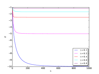
(a) for particles

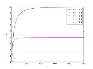
(b) for anti-particles

Figure 1: Spectrum of energy $E$ versus quantum number $n$ for some different $\gamma$ values in both coordinate and momentum spaces.

Now, we are ready to discuss some interesting results that are not well comments in the literature. From this Figure, the asymptotic limits for both form of energies are $\frac{1}{\left|\gamma\right|}$ as in the non-relativistic case. These limits have been reproduced for both cases in Figure. 1. Following this figure, some remarks can be made:

• the modified scalar product is the origin of that the he spectrum exhibits saturation instead of growing infinitely,

• the analytical asymptotic limits are well depicted,

• the beginning of the saturation starts from a specific quantum number $N$.

• this saturation appears for the high levels contrary to what has been found in the non-relativistic case (33, 33).

In what follow, we (i) studied the influence of the dependence of the potential with energies on the Fisher and Shannon parameters $F$ , and (ii) checked the validity of Stam, Cramer–Rao and BBM uncertainly relations for some values of $\gamma$.

III The influence of the $\gamma$ parameter on the Fisher and Shannon information measures

III.1 Fisher information

The Fisher information is a quality of an efficient measurement procedure used for estimating ultimate quantum limits. It was introduced by Fisher as a measure of intrinsic accuracy in statistical estimation theory but its basic properties are not completely well known yet, despite its early origin in 1925. Also, it is the main theoretic tool of the extreme physical information principle, a general variational principle which allows one to derive numerous fundamental equations of physics: Maxwell equations, the Einstein field equations, the Dirac and Klein-Gordon equations, various laws of statistical physics and some laws governing nearly incompressible turbulent fluid flows (34, 34, 35, 36, 37, 38). Fisher information has been very useful and has been applied in different areas in quantum physics (39, 39, 40, 41, 42, 43, 44, 46, 47, 48, 49, 50, 51, 52)

In our case: the Fisher information of one-dimensional Klein-Gordon oscillator with energy-dependent potential is

$$F_{x}=\int\rho_{n}\left(x,E\right)\left[\frac{d\text{ln}\left(\rho_{n}\left(x,E\right)\right)}{dx}\right]^{2}dx.$$ (11)

By using the properties of the Hermite functions properties, we found that

$$\begin{array}[]{c}F_{x}=\underset{I}{\underbrace{C_{n}^{2}\int_{-\infty}^{+\infty}\left(16n^{2}E\right)H_{n}^{2}\left(\sqrt{\lambda}x\right)\exp\left(-\lambda x^{2}\right)dx}}+\underset{II}{\underbrace{C_{n}^{2}\int_{-\infty}^{+\infty}-\left(16n\lambda E+8n\gamma\right)x\left(H_{n}^{2}\left(\sqrt{\lambda}x\right)\exp\left(-\lambda x^{2}\right)\right)dx}}+\\ \underset{III}{\underbrace{C_{n}^{2}\int_{-\infty}^{+\infty}\left(4\lambda^{2}E-8n^{2}\gamma+4\gamma\lambda\right)x^{2}\left(H_{n}^{2}\left(\sqrt{\lambda}x\right)\exp\left(-\lambda x^{2}\right)\right)dx}}+\underset{IV}{\underbrace{C_{n}^{2}\int_{-\infty}^{+\infty}8n\lambda\gamma x^{3}\left(H_{n}^{2}\left(\sqrt{\lambda}x\right)\exp\left(-\lambda x^{2}\right)\right)dx}}+\\ \underset{V}{\underbrace{C_{n}^{2}\int_{-\infty}^{+\infty}-2\omega_{E}^{2}\gamma x^{4}\left(H_{n}^{2}\left(\sqrt{\lambda}x\right)\exp\left(-\lambda x^{2}\right)\right)dx}}+\underset{VI}{\underbrace{C_{n}^{2}\int_{-\infty}^{+\infty}\left(\frac{\gamma^{2}x^{2}}{\left(E-\frac{1}{2}\gamma x^{2}\right)}\right)\left(H_{n}^{2}\left(\sqrt{\lambda}x\right)\exp\left(-\lambda x^{2}\right)\right)dx}}\end{array}$$ (12)

The evaluation of different terms giv

$$I \rightarrow C_{n}^{2}16n^{2}E2^{n}n!\frac{\sqrt{\pi}}{\sqrt{\lambda}},$$

$$II \rightarrow 0,$$

$$III \rightarrow C_{n}^{2}\left(4\lambda^{2}E-8n^{2}\gamma+4\gamma\lambda\right)\frac{1}{\lambda}2^{n}n!\frac{\sqrt{\pi}}{\sqrt{\lambda}}\left(n+\frac{1}{2}\right),$$

$$IV \rightarrow 0,$$

$$V \rightarrow-C_{n}^{2}2\gamma 2^{n}n!\frac{\sqrt{\pi}}{\sqrt{\lambda}}\left[\frac{\left(2n+1\right)^{2}+2}{4}\right].$$

The last term

$$VI \rightarrow C_{n}^{2}\int_{-\infty}^{+\infty}\left(\frac{\gamma^{2}x^{2}}{\left(E-\frac{1}{2}\gamma x^{2}\right)}\right)\left(H_{n}^{2}\left(\sqrt{\lambda}x\right)\exp\left(-\lambda x^{2}\right)\right)dx,$$

is calculate numerically.

Hence, the final form of the Fisher parameter is written by :

$$\begin{array}[]{c}F_{x}=\left(E-\frac{\gamma}{2\sqrt{1+\gamma E}}\left(n+\frac{1}{2}\right)\right)^{-1}\left\{16n^{2}E+\left(4\left(1+\gamma E\right)E-8n^{2}\gamma+4\gamma\sqrt{1+\gamma E}\right)\frac{1}{\sqrt{1+\gamma E}}\left(n+\frac{1}{2}\right)-2\gamma\left[\frac{\left(2n+1\right)^{2}+2}{4}\right]\right\}+\\ \frac{1}{2^{n}n!}\frac{\left(1+\gamma E\right)^{\frac{1}{4}}}{\sqrt{\pi}}\left(E-\frac{\gamma}{2\sqrt{1+\gamma E}}\left(n+\frac{1}{2}\right)\right)^{-1}\int_{-\infty}^{+\infty}\left(\frac{\gamma^{2}x^{2}}{\left(E-\frac{1}{2}\gamma x^{2}\right)}\right)\left(H_{n}^{2}\left(\sqrt{\lambda}x\right)\exp\left(-\lambda x^{2}\right)\right)dx\end{array}$$ (13)

Let’s now go to the momentum space: in this case we have

$$F_{p}=\int\rho_{n}\left(p_{x},E\right)\left[\frac{d\text{ln}\left(\rho_{n}\left(p_{x},E\right)\right)}{dp_{x}}\right]^{2}dp_{x}.$$ (14)

After some calculations, we obtain

$$\begin{array}[]{c}F_{p}=\underset{I}{\underbrace{C_{n}^{2}\int_{-\infty}^{+\infty}\left(16n^{2}E\right)H_{n}^{2}\left(\frac{p_{x}}{\sqrt{\lambda}}\right)\exp\left(-\frac{p_{x}^{2}}{\lambda}\right)dp_{x}}}+\underset{II}{\underbrace{C_{n}^{2}\int_{-\infty}^{+\infty}\left(\frac{2\gamma}{\lambda^{4}}-\frac{4nE}{\lambda}\right)p_{x}H_{n}^{2}\left(\frac{p_{x}}{\sqrt{\lambda}}\right)\exp\left(-\frac{p_{x}^{2}}{\lambda}\right)dp_{x}}}+\\ \underset{III}{\underbrace{C_{n}^{2}\int_{-\infty}^{+\infty}\left(\frac{4E}{\lambda^{2}}+\frac{8n^{2}\gamma}{\lambda^{4}}\right)p_{x}^{2}H_{n}^{2}\left(\frac{p_{x}}{\sqrt{\lambda}}\right)\exp\left(-\frac{p_{x}^{2}}{\lambda}\right)dp_{x}}}-\underset{IV}{\underbrace{C_{n}^{2}\int_{-\infty}^{+\infty}\frac{4n\gamma}{2\lambda^{5}}p_{x}^{3}H_{n}^{2}\left(\frac{p_{x}}{\sqrt{\lambda}}\right)\exp\left(-\frac{p_{x}^{2}}{\lambda}\right)dp_{x}}}+\\ \underset{V}{\underbrace{C_{n}^{2}\int_{-\infty}^{+\infty}\frac{4\gamma}{2\lambda^{6}}p_{x}^{4}H_{n}^{2}\left(\frac{p_{x}}{\sqrt{\lambda}}\right)\exp\left(-\frac{p_{x}^{2}}{\lambda}\right)dp_{x}}}+\underset{VI}{\underbrace{C_{n}^{2}\int_{-\infty}^{+\infty}\left(\frac{2\gamma^{2}p_{x}^{2}}{\lambda^{4}\left(2E\lambda^{4}+\gamma p_{x}^{2}\right)}\right)H_{n}^{2}\left(\frac{p_{x}}{\sqrt{\lambda}}\right)\exp\left(-\frac{p_{x}^{2}}{\lambda}\right)dp_{x}}}\end{array}$$ (15)

When we evaluate the terms appear in Eq. (15),

$$I \rightarrow C_{n}^{2}16n^{2}E2^{n}n!\sqrt{\pi}\sqrt{\lambda},$$

$$II \rightarrow 0,$$

$$III \rightarrow C_{n}^{2}\left(\frac{4E}{\lambda}+\frac{8n^{2}\gamma}{\lambda^{3}}\right)\frac{1}{\lambda}2^{n}n!\sqrt{\pi}\sqrt{\lambda}\left(n+\frac{1}{2}\right),$$

$$IV \rightarrow 0,$$

$$V \rightarrow C_{n}^{2}\frac{2\gamma}{\lambda^{4}}2^{n}n!\sqrt{\pi}\sqrt{\lambda}\left[\frac{\left(2n+1\right)^{2}+2}{4}\right],$$

we arrive at the final form of Fisher parameter where

$$\begin{array}[]{c}F_{p}=\left(E+\frac{\gamma}{2\lambda^{3}}\left(n+\frac{1}{2}\right)\right)^{-1}\left\{16n^{2}E+\left(\frac{4E}{\lambda}+\frac{8n^{2}\gamma}{\lambda^{3}}\right)\left(n+\frac{1}{2}\right)+\frac{2\gamma}{\lambda^{4}}\left[\frac{\left(2n+1\right)^{2}+2}{4}\right]\right\}\\ +\frac{1}{2^{n}n!\sqrt{\lambda}\sqrt{\pi}}\left(E+\frac{\gamma}{2\lambda^{3}}\left(n+\frac{1}{2}\right)\right)^{-1}\int_{-\infty}^{+\infty}\left(\frac{2\gamma^{2}p_{x}^{2}}{\omega_{E}^{4}\left(2E\lambda^{4}+\gamma p_{x}^{2}\right)}\right)H_{n}^{2}\left(\frac{p_{x}}{\sqrt{\lambda}}\right)\exp\left(-\frac{p_{x}^{2}}{\lambda}\right)dp_{x}.\end{array}$$ (16)

The last term in equation is calculate numerically.

III.2 Shannon entropy

Entropic measures provide analytic tools to help us to understand correlations in quantum systems. Shannon has introduced entropy to measure the uncertainty. Now, it has become a universal concept in statistical physics. The Shannon entropy has finding applications in several branches of physics because of its possible applications in a wide range of area (see Ref. 53, 53 and references therein).

The position space information entropies for the one-dimensional can be calculated by using

$$S_{x}=-\int\left|\psi\left(x\right)\right|^{2}\ln\left|\psi\left(x\right)\right|^{2}dx,$$ (17)

In our case, the above equation becomes

$$S_{x}=-\int\rho_{n}\left(x,\gamma\right)\ln\rho_{n}\left(x,\gamma\right)dx,$$ (18)

with $\rho_{n}\left(x,\gamma\right)$ is defined by the equations (7) and (8). In general, explicit derivations of the information entropy are quite difficult. In particular, the derivation of analytical expression for the $S_{x}$ is almost impossible.The overcome this difficulties, we (i) use a numerical calculation of this integral, and (ii) represent the Shannon and Fisher information entropy densities, respectively,

The form of this parameter, in the momentum space, is written by

$$S_{p}=-\int\rho_{n}\left(p_{x},E\right)\text{ln}\rho_{n}\left(p_{x},E\right)dp_{x}.$$ (19)

III.3 Results and discussions

In Figure. 2,

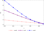
(a) coordinate space

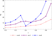
(b) momentum space

Figure 2: Fisher information of one-dimensional Klein-Gordon oscillator versus $\gamma$ for both coordinate and momentum spaces.

we show the Fisher parameter versus a $\gamma$ for both coordinate and momentum spaces: the case of coordinate space, $F_{x}$ decreases contrarily, in the momentum space where it increases. Moreover, this situation is inverted in the Figure. 3

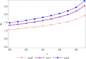
(a) coordinate space

(b) momentum

Figure 3: Shannon entropy of one-dimensional Klein-Gordon oscillator versus $\gamma$ for both coordinate and momentum spaces.

: the Shannon parameter increases in the $\left\{x\right\}$ configuration, whereas it decreases in the $\left\{p\right\}$ configuration. We note here, that these behavior is the same for the particles and anti-particles.

The information entropy and fisher densities are defined as,

$$\left(\rho_{F}\right)_{\left\{a\right\}}=\rho_{n}\left(a,E\right)\left[\frac{d\text{ln}\left(\rho_{n}\left(a,E\right)\right)}{da}\right]^{2},$$ (20)

for Fisher information, and

$$\left(\rho_{S}\right)_{\left\{a\right\}}=\rho_{n}\left(a,E\right)\text{ln}\rho_{n}\left(a,E\right),$$ (21)

for the Shannon entropies: $\left\{a\right\}$ denotes the appropriate configuration 54, 54, 55. The behavior of $\left(\rho_{F}\right)_{\left\{a\right\}}$ and $\left(\rho_{S}\right)_{\left\{a\right\}}$ is illustrated In Figures. 4 and 5 for $n=0,1,3$ and several values of the parameter $\gamma$

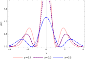
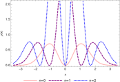
(a) coordinate space

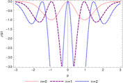
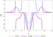
(b) momentum space

Figure 4: Fisher densities versus $x$.

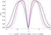
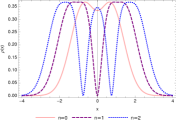
(a) coordinate space

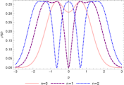
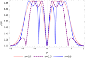
(b) momentum space

Figure 5: Shannon densities versus $p_{x}$.

Now, we are ready the discuss the Heisenberg uncertainly relation (HUR) and it’s analogue in the framework of quantum information: the HUR in quantum mechanics is an inequality between position and momentum. In recent years, a new uncertainty principles are introduced, and they are originate from the information theory: let us mention that this information-theoretic quantity and its quantum extension, not yet sufficiently well known for physicists, has been used to set up a number of relevant inequalities such as Stam and Cramer–Rao and uncertainty relations. The Cramer-Rao inequality belongs to a natural family of information-theoretic inequalities which play a relevant role in a great variety of scientific and technological fields ranging from probability theory, communication theory, signal processing and approximation theory to quantum physics of D -dimensional systems with a finite number of particles (56, 56, 57, 58, 59, 60, 61).

Also, the Fisher information of single-particle systems has been only recently determined in closed form in terms of the quantum numbers characterizing the involved physical state for both position and momentum spaces. These relevant inequalities which involve the Fisher information in a given space (Cramer–Rao) or the conjugate (Stam) space . They are the Stam uncertainty relations (53, 53)

$$F_{x}\leq 4\left\langle p^{2}\right\rangle,\,F_{p}\leq 4\left\langle x^{2}\right\rangle,$$ (22)

and the Cramer–Rao inequalities

$$F_{x}\geq\frac{1}{\left\langle x^{2}\right\rangle},\,F_{p}\geq\frac{1}{\left\langle p^{2}\right\rangle}.$$ (23)

In addition, for a general monodimensional systems we have that

$$F_{x}F_{p}\geq 4.$$ (24)

Table. 1

Table 1: Numerical results for the uncertainty relation and Fisher information and Shannon entropy of 1D Klein-Gordon oscillator with energy-dependent potential.

$n$	$\gamma$	$\left\langle x^{2}\right\rangle$	$\triangle x$	$\left\langle p_{x}^{2}\right\rangle$	$\triangle p$	$\triangle x\triangle p$	$F_{x}$	$F_{p}$	$F_{x}F_{p}$	$S_{x}$	$S_{p}$	$S_{x}+S_{p}$
	0	0.5000	0,7071	0.5000	0,7071	0.5000	2.0000	2.0000	4.0000	1.0724	1.0724	2.1448
	-0.16	0.5918	0,7693	0.4080	0,638	0.4908	1.69165	2.4516	4.1472	1.1561	0.9707	2.1268
	-0.32	0.7136	0,8447	0.2737	0,5232	0.4419	1.4026	3.7700	5.2878	1.2501	0.8054	2.0555
0	-0.48	0.8912	0,9440	0.0188	0,1371	0.1295	1.1276	6.9355	7.8205	1.3608	0.7162	2.0770
	-0.64	1.1842	1,0882	0.4410	0,6641	0.7227	0.8607	8.2659	7.1145	1.5014	0.9599	2.4613
	-0.80	1.8090	1,3450	0.6658	0,8160	1.0975	0.5927	12.2000	7.2311	1.7082	1.0184	2.7266
	0	1.5000	1,2247	1,5	1,2247	1.5000	6.0000	6.0000	36.0000	1.3427	1.3427	2.6854
	-0.16	1.8392	1,3562	1,17526	1,0842	1.4704	4.8935	7.6593	37.4804	1.4434	1.2167	2.6601
	-0.32	2.3685	1,5390	0,480699	0,6933	1.0670	3.8012	13.4774	51.2303	1.5644	1.0148	2.5792
1	-0.48	3.2837	1,8121	1,36547	1,1685	2.1175	2.7485	6.2457	17.1663	1.7147	1.2308	2.9455
	-0.64	5.1536	2,2702	1,02251	1,0112	2.2956	1.7716	13.5291	23.9682	1.9122	0.8693	2.7815
	-0.80	10.4112	3,2266	0,533192	0,7302	2.3561	0.9166	22.3000	20.4402	2.2096	0.5957	2.8053
	0	2,5	1,5811	2.5000	1,5811	2.5000	10.0000	10.0000	100.0000	1.4986	1.4986	2.9972
	-0.16	3,23687	1,7991	1.7994	1,3414	2.4133	7.7103	13.8006	106.4068	1.6128	1.3503	2.9631
	-0.32	4,51644	2,1252	0.9625	0,9811	2.0850	5.4827	17.7237	97.1737	1.7513	1.3525	3.1038
2	-0.48	7,00704	2,6471	1.7410	1,3195	3.4928	3.4664	9.8800	34.2480	1.9195	1.0208	2.9403
	-0.64	12,5885	3,5480	1.0710	1,0349	3.6718	1.8689	19.9000	37.1911	2.1301	0.6893	2.8194
	-0.80	29,3421	5,4168	0.4937	0,7026	3.8085	0.7776	48.9000	38.0261	2.2452	0.3027	2.5479

shows a numerical results for the uncertainty relation and Fisher information measure of 1D Klein-Gordon oscillator for three levels ($n=0,1,2$) for some choice of parameter $\gamma$. Following this Table, we observe that

• the Stam inequalities, and Cramer–Rao ones are fulfilled,

• the following relation

  $$F_{x}F_{p}\geq 4,$$ (25)

  with D is the space dimension is well-established.

• and, finally, as the results indicate that the sum of the entropies is in consistency with BBM inequality, possesses the stipulated that

  $$S_{x}+S_{p}\geq D\left(1+\text{ln}\pi\right).$$ (26)

  In our case, we have $S_{x}+S_{p}\geq 2.14422$.

IV CONCLUSION

The present work is devoted to energy dependent potentials. We studied the physical characteristics of a 1D Klein-Gordon oscillator with energy dependent-potential. We first obtained the wave functions and the energy spectra of the system in an exact analytical manner. As a first result, we showed that the energy dependence affects essentially the eigenfunctions and eigenvalues. Especially, we observed a saturation in curves of energy spectrum. Also the presence of the energy–dependent potential in a wave equation leads to the modification of the scalar product, which was necessary to ensure the conservation of the norm. In this context, Fisher information and Shannon entropy, some expectation values, and some uncertainty principles were evaluated: in this way, we have studied the influence of the parameter $\gamma$ on Shannon entropy and Fisher information uncertainty relations, and checked the validity of BBM inequality. We showed that the numerical results in the information entropic is predicted by the BBM inequality $S_{x}+S_{p}\geq 1+\text{ln}\pi$, for some values of parameter $\gamma$ . In conclusion, the uncertainly relations given by quantum information theory, can be extended normally to the case of the potentials which depend with energy.

References

-
(1)
H. Snyder and J. Weinberg, Phys. Rev. 57,
307 (1940);
I. Schiff, H. Snyder and J.Weinberg, Phys. Rev. 57, 315 (1940). - (2) A.M. Green, Nucl. Phys. 33 ,218 (1962).
- (3) W. Pauli, Z. Physik. 601, 43 (1927).
- (4) H.A. Bethe and E.E. Salpeter, Quantum theory of One- and Two-Electron Systems, Handbuch der Physik, Band XXXV, Atome I, Springer Verlag, Berlin-G¨ottingen-Heidelberg, (1957).
- (5) H. Sazdjian, J. Math. Phys. 29, 1620 (1988).
- (6) J. Formanek, J. Mares and R. Lombard, Czech. J. Phys. 54, 289 (2004).
- (7) J. Garcia-Martinez, J. Garcia-Ravelo, J. J. Pena and A. Schulze-Halberg, Phys. Lett. A. 373, 3619 (2009).
- (8) R. Lombard, An-Najah Univ. J. Res. (N. Sc.). 25, 49 (2011).
- (9) H. Hassanabadi, S. Zarrinkamar and A. A. Rajabi, Commun. Theor. Phys. 55, 541 (2011).
- (10) H. Hassanabadi, E. Maghsoodi, R. Oudi, S. Zarrinkamar, H. Rahimov, Eur. Phys. J. Plus. 127, 120 (2012).
- (11) R. J. Lombard and J. Mares, Phys. Lett. A. 373, 426 (2009).
-
(12)
R. Yekken and R. J. Lombard, J. Phys. A: Math. Theor.
43, 125301 (2010);
R. Yekken, Phd Thesis, Université des Sciences et de la Technologie Houari Boumediene d’Alger, Algeria, (2009). - (13) A. Schulze-Halberg, Cent. Eur. J. Phys. 9, 57 (2011).
- (14) R. J. Lombard, J. Mares and C. Volpe, arXiv:hep-ph/0411067v1.
- (15) H. Hassanabadi, S. Zarrinkamar, H. Hamzavi and A. A. Rajabi, Arab. J. Sci. Eng. 37, 209 (2012).
- (16) D. Itô, K. Mori and E. Carriere, Nuovo Cimento A, 51, 1119 (1967).
- (17) M. Moshinsky and A. Szczepaniak, J. Phys. A: Math. Gen, 22, L817 (1989).
- (18) R. P. Martinez-y-Romero and A. L. Salas-Brito, J. Math. Phys, 33 , 1831 (1992).
- (19) M. Moreno and A. Zentella, J. Phys. A: Math. Gen, 22 , L821 (1989).
- (20) J. Benitez, P. R. Martinez y Romero , H. N. Nunez-Yepez and A. L. Salas-Brito,Phys. Rev. Lett, 64, 1643–5 (1990).
- (21) C. Quesne and V. M. Tkachuk, J. Phys. A: Math. Gen, 41 , 1747–65 (2005).
- (22) A. Boumali and H. Hassanabadi, Eur. Phys. J. Plus. 128, 124 (2013).
- (23) A. Boumali and H. Hassanabadi, Z. Naturforschung A. 70, 619-627 (2015).
- (24) A. Boumali, EJTP 12, No. 32,1-10 (2015).
- (25) A. Boumali, Phys. Scr. 90, 045702 (2015).
- (26) P. Strange, L.H. Ryder, Phys. Lett. A , 380, 3465-3468 (2016).
- (27) A. Franco-Villafane, E. Sadurni, S. Barkhofen, U. Kuhl, F. Mortessagne, and T. H. Selig- man, Phys. Rev. Lett. 111, 170405 (2013).
- (28) A. J. Stam A J Inf. Control 2, 101 (1959).
- (29) T. M. Cover and J. A.Thomas, Elements of Information Theory,Wiley, NewYork,(1991).
- (30) O. Johnson, Information Theory and the Central Limit Theorem, Imperial College Press, London (2004).
- (31) Iwo Biatynicki-Birula and Jerzy Mycielski, Commun, math. Phys. 44, 129–132 (1975).
- (32) A. Boumali, A. Hafdallah and A. Toumi, Phys. Scr. 84, 037001 (2011).
- (33) A. Boumali, S. Dilmi, S. Zare and H. Hassanabdi, arXiv:1607.02123v2 (2016)
- (34) B.R. Frieden, Am. J. Phys. 57, 1004 (1989).
- (35) B.R. Frieden, Phys. Rev. A. 41, 4265 (1990).
- (36) B.R. Frieden, Opt. Lett. 14, 199 (1989).
- (37) B. R. Frieden, Physica. A. 180, 359-385 (1992).
- (38) B. R. Frieden and B. H. Soffer, Phys. Rev. E. 52, 2274-2286 (1995).
- (39) D.X. Macedo and I. Guedes, Physica. A. 434, 211-219 (2015).(2008).
- (40) P.A. Bouvrie, J.C. Angulo and J.S. Dehesa, Physica. A. 390, 2215-2228 (2011).
- (41) J. S. Dehesa, S. López-Rosa, and B. Olmos, J. Math. Phys. 47, 052104 (2006).
- (42) B J Falaye, K J Oyewumi, S M Ikhdair and M Hamzavi, Phys. Scr. 89 , 115204 (2014).
- (43) V. Aguiar and I. Guedes, Phys. Scr. 90, 045207 (2015).
- (44) B.J. Falayea, F.A. Serranob and Shi-Hai Dongc, Phys. Lett. A. 380, 267–271 (2016).
- (45) Juan He , Zhi-Yong Ding and Liu Ye, Physica. A, (2016).
- (46) M. Ghafourian and H. Hassanabadi, J. Korean. Phys. Soc, 68, 1-4 (2016),
- (47) G. H. Sun, S. H. Dong and S. Naad, Ann. Phys. 525, 934 (2013).
- (48) G. H. Sun, M. Avila Aoki and S. H. Dong, Chin. Phys. B 22, 050302 (2013).
- (49) S. Dong, G. H. Sun, S. H. Dong and J. P. Draayer, Phys. Lett. A 378, 124 (2014).
- (50) G. H. Sun, S.H. Dong, K. D. Launey, T. Dytrych and J. P., Draayer, Int. J. Quantum Chem. 115, 891 (2015).
- (51) R. Valencia-Torres, G. H. Sun and S. H. Dong, Phys. Scr. 90, 035205 (2015).
- (52) B. J. Falaye, F. A. Serrano and S. H. Dong, Phys. Lett. A 380, 267 (2016).
- (53) J S Dehesa, R González-Férez and P Sánchez-Moreno, J. Phys. A: Math. Theor. 40,1845 (2007).
- (54) J-F Bercher, J. Phys. A: Math. Theor. 45, 255303 (2012).
- (55) S. Zare and H. Hassanabadi, Advances in High Energy Physics Volume 2016, Article ID 4717012,
- (56) Aparna Saha, B Talukdar and Supriya Chatterjee, Eur. J. Phys. 38, 025103 (2017).
- (57) D Manzano 1,2,4 , R J Yáñez 1,3,4 and J S Dehesa, New. J. Phys. 12, 023014 (2010).
- (58) Jaime Sañudo and Ricardo López-Ruiz, J. Phys. A: Math. Theor. 41, 265303 (2008).
- (59) P Sánchez-Moreno, R González-Férez and J S Dehesa, New. J. Phys. 8, 330 (2006).(
- (60) Seyede Amene Najafizade, Hassan Hassanabadi, and Saber Zarrinkamar, Can. J. Phys. 94, 1085-1092 (2016).
- (61) J.S. Dehesa, A.R. Plastino, P. Sanchez-Moreno, C. Vignat, Appl. Math. Lett. 25, 1689–1694 (2012).