A high order bound preserving finite difference linear scheme for incompressible flows
Abstract.
We propose a high order finite difference linear scheme combined with a high order bound preserving maximum-principle-preserving (MPP) flux limiter to solve the incompressible flow system. For such problem with highly oscillatory structure but not strong shocks, our approach seems to be less dissipative and much less costly than a WENO type scheme, and has high resolution due to a Hermite reconstruction. Spurious numerical oscillations can be controlled by the MPP flux limiter. Numerical tests are performed for the Vlasov-Poisson system, the 2D guiding-center model and the incompressible Euler system. The comparison between the linear and WENO type schemes will demonstrate the good performance of our proposed approach.
Keywords. High order linear scheme; MPP flux limiter; Incompressible transport equations.
1. Introduction
In this paper, we are interested in the numerical approximation of incompressible transport equations as
| (1.1) |
where represents the advection field and is a nonnegative density.
The typical example of application is the well known Vlasov-Poisson (VP) system arising in collisionless plasma physics. It describes the time evolution of particles under the effects of self-consistent electrostatic field and reads
| (1.2) |
is the distribution function in the phase space . is the electric field, which can be determined by the Poisson’s equation from an electric potential function
| (1.3) |
The charge density is defined as
Another example is the two dimensional guiding-center model, which describes the evolution of the charge density in a highly magnetized plasma in the transverse plane of a tokomak, is given by
| (1.4) |
where is a divergence free velocity. The two dimensional guiding center model can also be referred as an asymptotic model of the VP system by averaging in the velocity phase space, for details, see [22]. We notice that the guiding-center model (1.4) is in the same form as the two dimensional incompressible Euler equations in the vorticity stream function formulation, which describes the evolution of vortices in fluid hydrodynamics.
For all the models we mention above, they all have an transport equation coupled with a Poisson’s equation for the advection velocity, and moreover, the advection velocity is divergence free. In the following, we refer them as incompressible flow models.
Many numerical schemes have been proposed for solving these models, especially recently, high order schemes are very attractive due to their high resolutions for such problems with rich solution structures. For example, deterministic methods, there are finite difference, finite volume and finite element Eulerian methods [8, 37, 32, 40, 6, 14, 15, 41, 13, 39, 38], semi-Lagrangian methods [3, 34, 5, 25, 33, 18, 10, 26, 27, 28, 9, 24, 4, 31], and discontinuous Galerkin finite element methods [17, 42, 23, 7, 11, 19, 2], also see many other references therein. However, due to the highly oscillatory structure of such problems, linear type schemes for these problems would show significant spurious numerical oscillations, which might get worse with increased orders. Weighted essentially nonoscillotry (WENO) reconstruction, which was originally developed in the presence of both shocks and small fine structures for fluid hydrodynamics of hyperbolic conservation laws, see for example [29], is frequently adopted in most of the finite difference and finite volume Eulerian or semi-Lagrangian methods mentioned above. For WENO type schemes, we can often observe the good performance of the WENO reconstruction on suppressing spurious oscillations [25, 33, 37, 32, 40], which can also be seen from our examples in the numerical section. However, for incompressible flow problems, their solutions are highly oscillatory but without strong discontinuities. We might expect excessive usage of the WENO reconstruction, which is computationally more expensive than a pure linear type scheme and too dissipative for certain classes of problems [20], especially for high dimensional problems with long time simulations. Although hybrid approaches of coupling a linear scheme and a WENO scheme can save some cost from the WENO reconstruction, for example the very recent work [12] and references therein, they still focus on problems with strong discontinuities and WENO may not be avoided.
In this paper, we propose to solve the incompressible flow problems with a high order linear scheme without WENO reconstruction. Linear schemes have the following several good properties: (1) less dissipative: for example, it preserves the norm (also energy and entropy for the VP system) better than the WENO type scheme; (2) less costly and easier implementation: without WENO reconstruction, it saves a lot computational cost and can be easily implemented, especially when extended to high dimensional problems; (3) higher resolution if with a Hermite reconstruction. We adopt the scheme in [37] but with a Hermite linear reconstruction. In order to control the spurious numerical oscillations due to a linear type scheme, we seek to combine it with a newly developed high order bound preserving maximum-principle-preserving (MPP) flux limiter. The MPP flux limiter was first proposed by Xu et. al. [35, 21], and then improved by Xiong et. al. [32, 33]. It can be seen as a very weak limiter, which just pulls the numerical overshootings and undershootings back to its physical range, without excessive dissipating the solution within the range. Moreover, there is no further time step restriction on this MPP flux limiter from the original scheme for linear stabilities. We refer to [36] for a review of recent works on this bound preserving high order flux limiter. The coupling of the linear scheme and the MPP flux limiter keeps the original high order accuracy while maintaining a large CFL number. Due to the highly oscillatory but non discontinuous solutions of incompressible flow problems, the MPP flux limiter can serve as a necessary auxiliary tool for the linear scheme. The extra work from applying the MPP flux limiter at each final stage of a multi-stage Runge-Kutta time discretization, is much less than the WENO reconstruction. Numerical experiments, especially the bump-on-tail instability of long time simulation and the Kelvin-Helmoholtz instability of the 2D guiding-center model are as benchmark tests, will be performed to demonstrate the good performance of our proposed approach.
The rest of the paper is organized as follows. In Section 2, we will describe the conservative finite difference scheme with both linear and WENO reconstructions, for the completeness of comparison in the numerical section. The bound preserving MPP flux limiter will also be briefly reviewed. In Section 3, numerical experiments including the VP system, the Kelvin-Helmholtz instability of the 2D guiding center model and the incompressible Euler system will be studied. Conclusions are made in Section 4.
2. Finite difference scheme with Hermite reconstruction
In this section, we will describe our scheme to solve the VP system (1.2)-(1.3), the 2D guiding-center model (1.4) as well as the incompressible Euler system. Here we just consider for the VP system, in common we will have a 2D transport equation with a divergence free velocity, coupled with a Poisson’s type equation, which is 1D for the VP system, and 2D for the other two. In the following, we will take the 2D guiding-center model (1.4) as an example to describe our schemes. The other two models can be applied similarly.
We propose a finite difference scheme with a Hermite linear reconstruction for solving the 2D conservative transport equation. We adopt the scheme developed by Filbet and Yang [37], which has a Hermite WENO reconstruction. In the following, we will briefly recall the 2D conservative finite difference scheme and describe both the Hermite linear and WENO reconstructions. We note that the smooth indicators for the Hermite WENO reconstruction are modified as compared to [37]. The Poisson’s equation for the electric potential function will be solved by fast Fourier transform (FFT) for periodic boundary condition on an interval in one-dimension (1D) or periodic boundary conditions on a rectangular domain in two-dimension (2D), which will be omitted here. We refer to [37] for more details.
2.1. Conservative finite difference scheme
We consider the 2D transport equation in a conservative form
with such that and . For simplicity, we assume a uniform discretization of the computational domain with grid points
where the mesh sizes are and for . A conservative finite difference scheme with Euler forward time discretization is defined as follows:
| (2.1) |
where the time step is . is the numerical value at time level on the grid point . , are the numerical fluxes in the and directions respectively.
2.2. Hermite linear reconstruction
For a finite difference scheme (2.1), the numerical fluxes and are reconstructed dimension by dimension. Here we will take a 1D transport equation to illustrate on how to obtain a flux by a Hermite linear reconstruction. and are obtained in this way along each of its own direction. The Hermite linear reconstruction is what we propose in this paper. A corresponding Hermite WENO reconstruction will be described in the next subsection, which is used for the comparison in the numerical section.
Let us consider a prototype 1D conservative transport equation
| (2.2) |
with velocity and a uniform discretization with mesh size for . A conservative finite difference scheme for (2.2) can be written as
where is the numerical point value at time level on the grid point . can be chosen as an upwind numerical flux, which is
are fluxes reconstructed from by a Hermite linear reconstruction, from the left and right sides of respectively, where is the numerical velocity approximating . For simplicity, we drop the superscript for and is simply reconstructed by
| (2.3) |
where the derivative of the primitive function is given by a 6th order central difference approximation
| (2.4) |
can be obtained in mirror symmetric with respect to .
2.3. Hermite WENO reconstruction
Now we will describe a fifth order Hermite WENO reconstruction to compute corresponding to (2.3). The procedure is outlined as follows. can also be obtained in mirror symmetric with respect to . We drop the superscript for and we have
| (2.5) |
The three polynomials , and evaluating at are
whereas the weights , and are the nonlinear WENO weights and determined according to the smoothness indicators
In order to match (2.3), the linear coefficients are and . The small parameter is to avoid the denominator to be .
To evaluate the smooth indicators , and , we measure them on the cell instead of as in [37]. In this way, the smooth indicators are symmetric with respect to , as we can see below:
2.4. High order Runge-Kutta time discretization
The first order Euler forward time discretization (2.1) can be generalized to high order Runge-Kutta (RK) time discretization [30]. For example, if we write (2.1) in the following form
here the subscripts for are dropped and the operator denotes the spatial discretization, then a 4th order RK time discretization can be written as
| (2.6) |
with a CFL number for linear stability [30]. The last stage of (2.6) can be written in the same form as (2.1), which is
| (2.7) |
where the numerical flux is accumulated from all formal stages, that is
where is the numerical flux at the corresponding -th stage, and the subscript is dropped for clarity. is defined similarly.
2.5. Bound preserving MPP flux limiter
For a high order bound preserving limiter, we adopt the parametrized maximum-principle-preserving (MPP) flux limiter developed in [32, 33]. The MPP flux limiter is only applied at the final stage of (2.6), that is (2.7). Due to the same form of (2.1) and (2.7), the MPP flux limiter is defined as a convex combination of a first order monotone flux and the high order flux in (2.7). In the following, we first describe a first order monotone MPP scheme for a general incompressible flow system, then we recall a specific first order monotone MPP scheme developed in [32] for the incompressible flow system with the Poisson’s equation.
For a general incompressible flow system with divergence free condition
| (2.8) |
a first order scheme can be defined as
| (2.9) |
where and . If the scheme (2.9) is a consistent discretization to (2.8), we have the following statement:
Proposition 2.1.
Proof.
We can rewrite the first equation in the scheme (2.9) to be
| (2.12) |
with
It is easy to check that are all positive if the two conditions (2.10) and (2.11) are satisfied. Moreover,
due to the enforced discrete divergence free condition in (2.9). Since (2.12) is a convex combination, so it is monotone and MPP. ∎
A specific first order monotone MPP scheme depends on how to choose and . By using a potential function , where , a first order monontone MPP scheme with Lax-Friedrichs flux defined in [32] is to take:
| (2.13) |
where
In this paper, the potential function is obtained by solving the Poisson’s equation with FFT.
Now to describe the MPP flux limiter, we write the first order monotone MPP scheme in a conservative flux difference form
| (2.14) |
with
| (2.15) |
and are first order monotone numerical fluxes. Similarly, (2.7) is
| (2.16) |
In order to ensure maximum principle, we are looking for type of limiters
| (2.17) |
such that
| (2.18) |
(2.17) and (2.18) form coupled inequalities for the limiting parameters . We will need to find a group of numbers , such that (2.18) is satisfied with
This is achieved in a decoupled way for the minimum and maximum parts. For the maximum value case, we let
| (2.19) |
and denote
| (2.20) |
then (2.18) can be rewritten as
| (2.21) |
We shall now focus on decoupling the inequalities (2.21): for the single node ,
-
(1)
Identify positive values out of the four locally defined numbers , , , ;
-
(2)
Corresponding to those positive values, collectively, the limiting parameters can be defined. For example, if and , then
(2.22)
that is, all high order fluxes which possibly contribute (beyond that of the first order fluxes, which is not good) to the overshooting or undershooting of the updated value shall be limited by the same scaling. Similarly we can find and also similarly for the minimum value case of and . Therefore the range of the limiting parameters satisfying MPP for a single node is defined by
| (2.23) |
Considering the limiters from neighboring nodes, finally we let
| (2.24) |
Substituting (2.24) into (2.17), our final scheme is (2.16) by replacing the fluxes from (2.17).
3. Numerical examples
In this section, we will apply the 5th order finite difference scheme with Hermite linear reconstruction (2.3) and (2.4), coupled with the bound preserving MPP flux limiter, which we denote as “HLinear5 MPP”, to test its good performance. The Hermite linear scheme without bound preserving MPP flux limiter is denoted as “HLinear5”, while those with Hermite WENO reconstruction (2.5) are denoted as “HWENO5 MPP” and “HWENO5” for with and without MPP flux limiter correspondingly. All the schemes without Hermite reconstruction, for example the one in [32], will be denoted as “WENO5 MPP” and “WENO5”, and the corresponding linear schemes as “Linear5 MPP” and “Linear5”, respectively. They will also be used for comparison in the following. The time step is taken as
where , and we take the CFL number to be in all the following tests.
We would emphasize that to apply the MPP limiter, the minimum and maximum values of the bounds are taken from the initial data, which can be explicitly determined for all the tests here.
3.1. Linear transport equations
Example 3.1.
We first take a 2D linear transport equation with initial condition
| (3.1) |
on the domain with periodic boundary conditions, to test the accuracy of the “HLinear5 MPP” and “HLinear5” schemes. The exact solution is
| (3.2) |
The solution is within . From Table 3.1, we can clearly observe undershootings without the MPP limiter, while with limiter the lower bound is well preserved (as is for the upper bound) and 5th order accuracy is maintained. We would mention that for all other schemes we considered in this section, the accuracies are all tested and perform similarly. We omit them to save space.
| N | error | order | error | order | ||
|---|---|---|---|---|---|---|
| WO | 32 | 5.00e-04 | – | 1.29e-03 | – | -0.001019 |
| 64 | 1.90e-05 | 4.72 | 4.91e-05 | 4.72 | -4.244e-05 | |
| 128 | 6.41e-07 | 4.89 | 1.68e-06 | 4.87 | -1.242e-06 | |
| 256 | 2.05e-08 | 4.97 | 5.35e-08 | 4.97 | -4.403e-08 | |
| WL | 32 | 5.16e-04 | – | 1.33e-03 | – | 0.0003958 |
| 64 | 1.90e-05 | 4.77 | 5.54e-05 | 4.59 | 5.522e-06 | |
| 128 | 6.41e-07 | 4.89 | 2.07e-06 | 4.74 | 9.832e-13 | |
| 256 | 2.05e-08 | 4.97 | 7.78e-08 | 4.73 | 1.712e-09 |
Then we take a 1D linear transport equation with highly oscillatory solutions. Here the initial condition is chosen to be
| (3.3) |
on the domain with periodic boundary condition, and the exact solution is
| (3.4) |
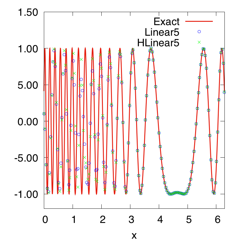
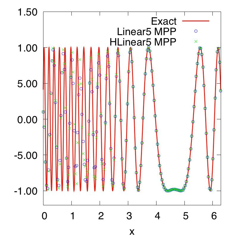
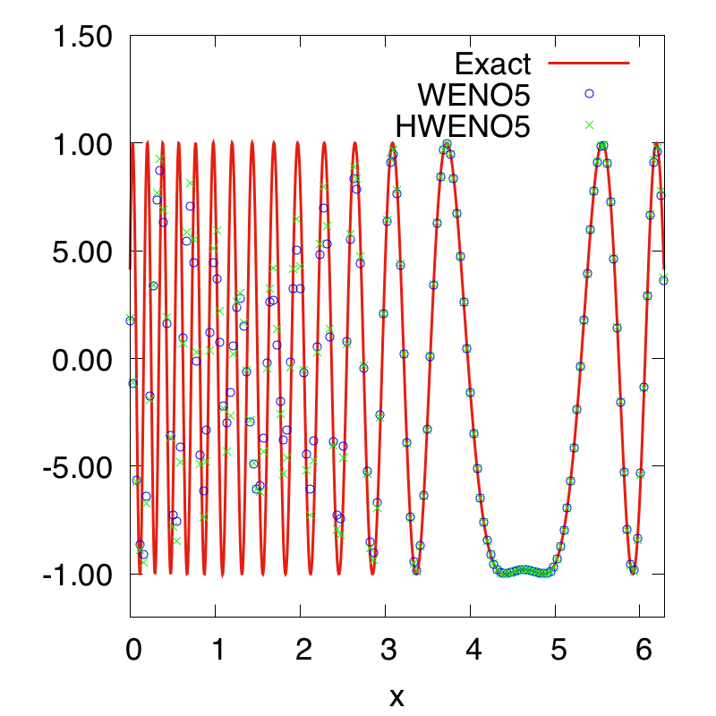
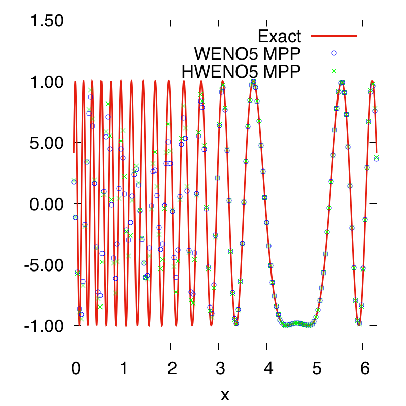
In Fig. 3.1, we show the results for both linear and WENO type schemes, without and with MPP limiter respectively. From the figures, we can observe that the “HLinear5” scheme has better resolution than the “Linear5” scheme, due to a Hermite reconstruction for such a highly oscillatory solutions, while linear schemes are better than WENO type schemes due to less dissipation. We can also see that the resolution of these schemes do not significantly affect by the MPP limiter, which is used to control the solutions within the global physical range . So in the following, we will focus on the “HLinear5” and “HLinear5 MPP” schemes, and compare them to their corresponding WENO type approaches, which are “HWENO5” and “HWENO5 MPP” respectively. We mainly would like to show that a 5th order linear scheme with a Hermite reconstruction and an MPP limiter, that is “HLinear5 MPP”, is a very good scheme for highly oscillatory solution without discontinuities.
 |
 |
| (a) | (b) |
 |
 |
| (c) | (d) |
3.2. Vlasov-Poisson system
In this subsection, we consider the VP system (1.2) and (1.3) with 1D in and 1D in , and periodic boundary condition in both directions. We take and use instead of for the special meaning of the argument here. The cut-off domain in the direction is taken to be if without specifications. The VP system preserves several norms, which should remain constant in time:
-
(1)
norm, :
(3.5) -
(2)
Energy:
(3.6) where is the electric field.
-
(3)
Entropy:
(3.7)
We will track the relative deviations of these quantities numerically to measure the quality of our numerical scheme. The relative deviation is defined to be the deviation away from the corresponding initial value divided by the magnitude of the initial value. The mass conservation over time is obvious for conservative schemes, which is the same as the norm when is positive, so only the norm is shown below. We would also note that for the VP system, although the minimum part is known as positivity preserving, however, due to a cut-off domain in the direction, the minimum value might be close to but above . We clearly indicate the minimum and maximum values from the initial data for the tests below.
Example 3.2.
(Accuracy test) We first consider the VP system with the following initial condition
| (3.8) |
and periodic boundary conditions on the computational domain , where , to test the accuracy of the schemes for this system. From the initial data, the solution should be within the range .
In Table 3.2, we show the and errors and orders for the “HLinear5” and “HLinear5 MPP” scheme respectively. For this example, th order accuracy can also be observed as mesh refinement. Without limiter, the solution of the distribution function does not preserve positivity, while with limiter, all values are above . Here we measure the errors on two consecutive mesh sizes by double refinement, since the exact solution is not explicitly available.
| error | order | error | order | |||
| WO | 64 | 1.66e-05 | – | 0.0004144 | – | -1.317e-06 |
| 128 | 6.83e-07 | 4.60 | 1.913e-05 | 4.44 | -2.197e-08 | |
| 256 | 2.54e-08 | 4.75 | 7.137e-07 | 4.75 | -1.777e-09 | |
| 512 | 8.29e-10 | 4.94 | 2.342e-08 | 4.93 | -5.535e-11 | |
| WL | 64 | 1.68e-05 | – | 0.0004177 | – | 1.59e-32 |
| 128 | 6.85e-07 | 4.62 | 1.915e-05 | 4.45 | 1.768e-34 | |
| 256 | 2.54e-08 | 4.75 | 7.136e-07 | 4.75 | 2.339e-35 | |
| 512 | 8.30e-10 | 4.94 | 2.342e-08 | 4.93 | 4.797e-36 |
Example 3.3.
(Strong Landau damping) We then consider the strong Landau damping with the initial condition:
| (3.9) |
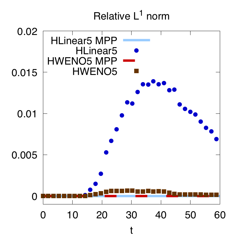
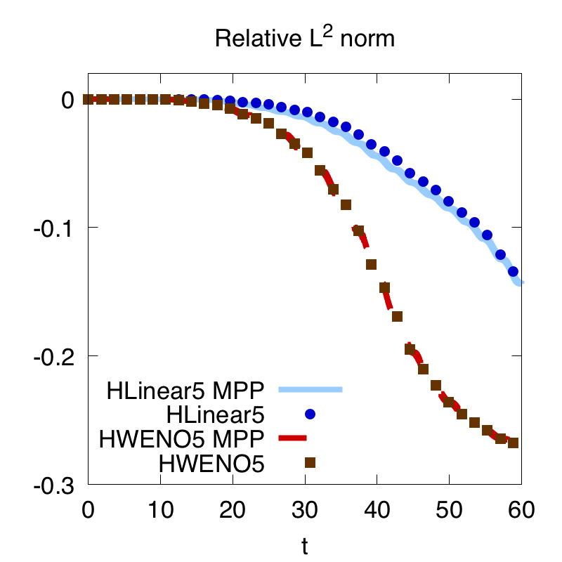
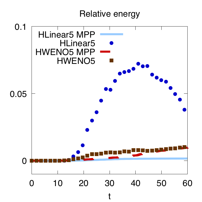
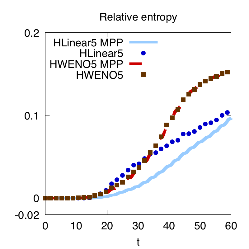
where and . The length of the domain in the x-direction is , which is similar in the following two examples. For this problem, from the initial data, the solution should be within the range . In Fig. 3.2, we plot the surface of the distribution function at in the range of . The mesh grid is . We can observe that without limiter, the solution can be negative (white spots), while negative values are eliminated by the scheme with limiter, similarly for the following examples. Then in Fig. 3.3, we show the time evolution of the electric field in norm and norm, the relative derivation of the discrete norm, norm, kinetic energy and entropy. From this figure, we can see that the electric field for all schemes are almost the same. The linear type scheme can preserve the norm and entropy better than the WENO type scheme, where the MPP limiter does not significantly affect these two quantities. However, for the norm and energy, the linear scheme without limiter performs much worse than the WENO type scheme, but after with limiter, it is the best. Especially for the energy, “HLinear5 MPP” is much better than all other schemes. This example has clearly show the good performance of our approach.
Example 3.4.
(Symmetric two stream instability) We now consider the symmetric two stream instability with the initial condition:
| (3.10) |
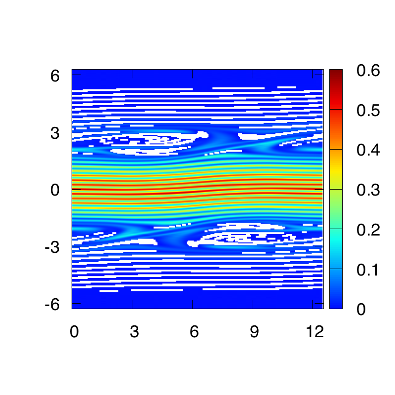
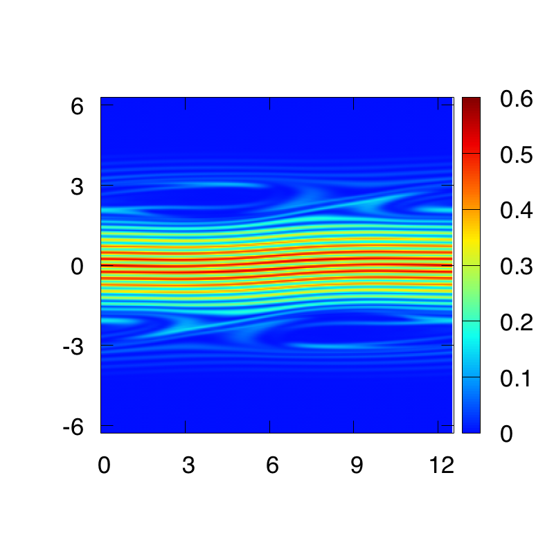
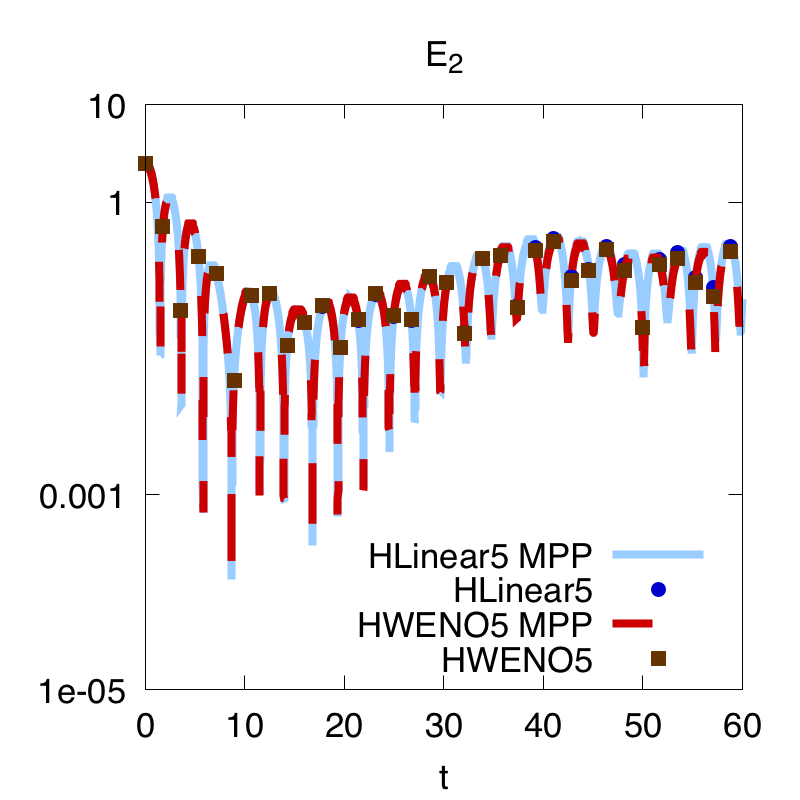
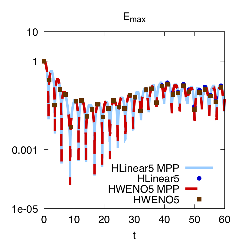
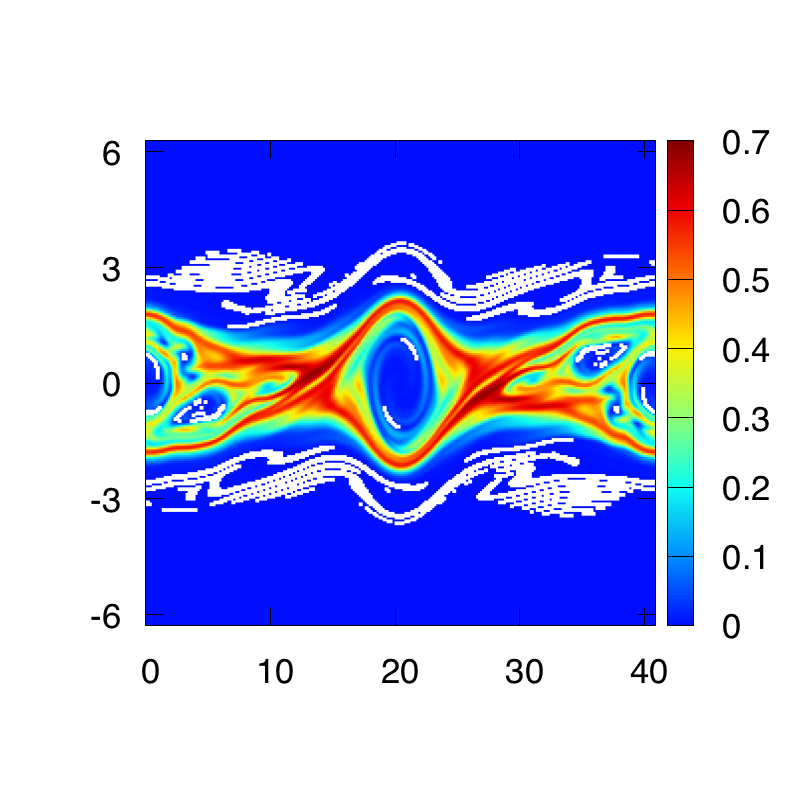
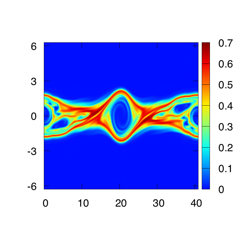
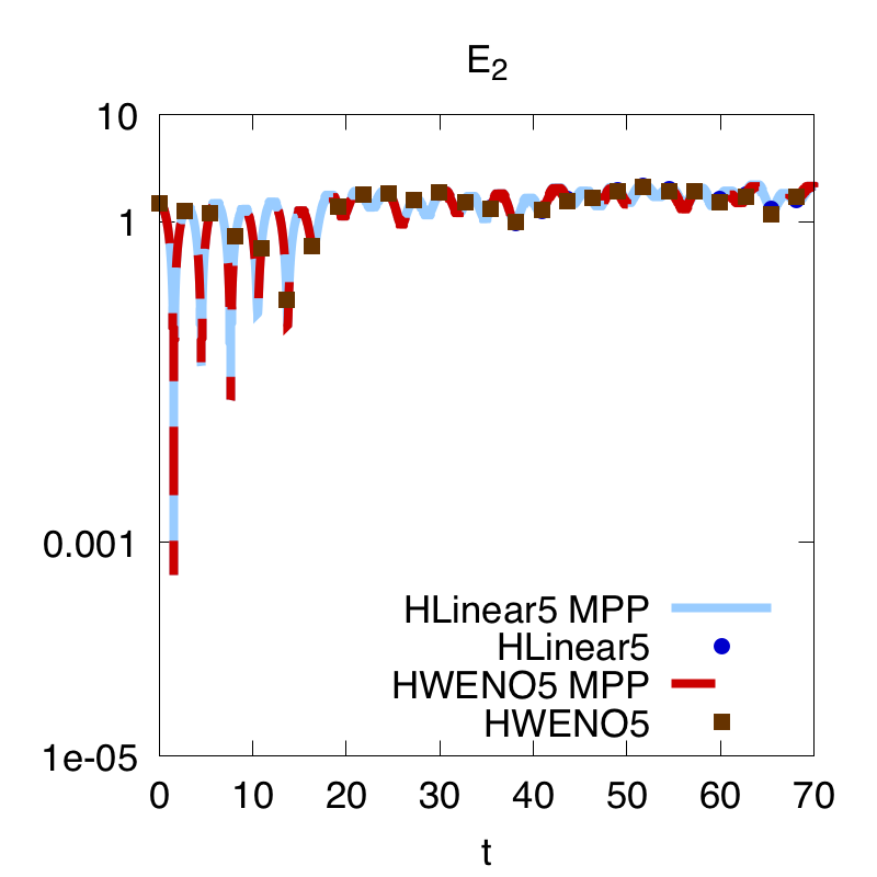
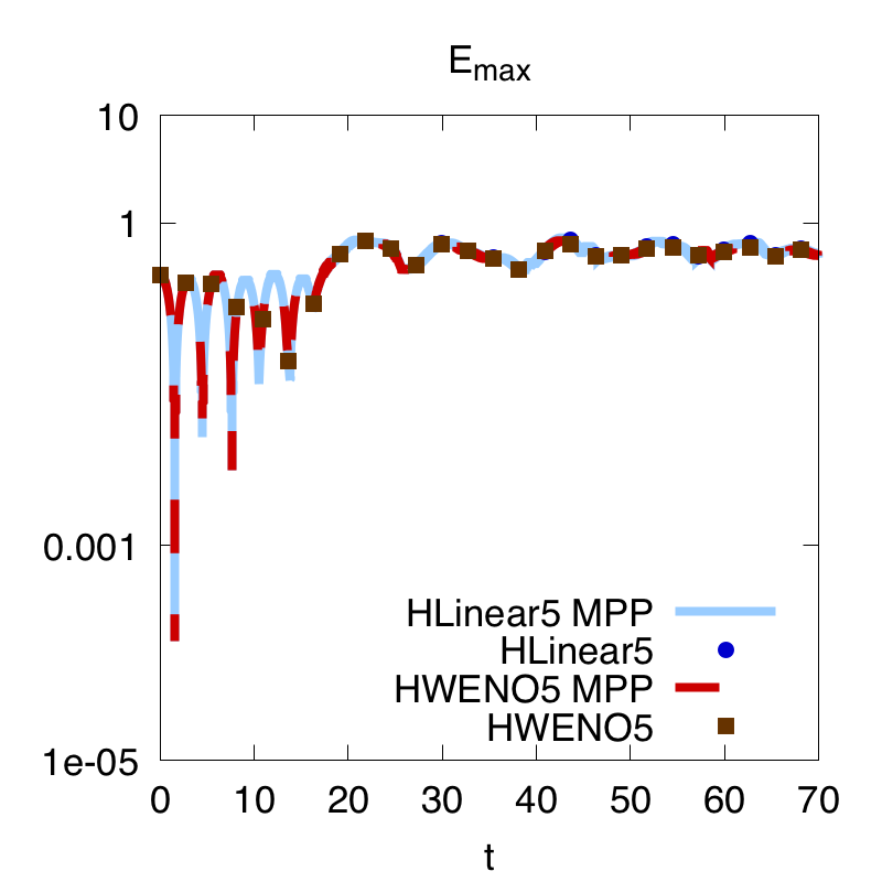
where , , and . Similarly, from the initial data, the minimum value of the solution is taking and in (3.10), while the maximum value is taking or , and . We plot the numerical solution at in Fig. 3.4 for the “HLinear5” and “HLinear5 MPP” schemes respectively. The mesh grid is . We can also clearly observe that without limiter, the solution becomes negative, which, however, can be eliminated by the scheme with limiter. We show the time evolution of the electric field in norm and norm, the relative derivation of the discrete norm, norm, kinetic energy and entropy in Fig. 3.5. Similar results as the last example are obtained.
Example 3.5.
(Bump-on-tail instability) We consider the bump-on-tail instability problem [1, 33] with the initial condition as
| (3.11) |
where the bump-on-tail distribution is
| (3.12) |
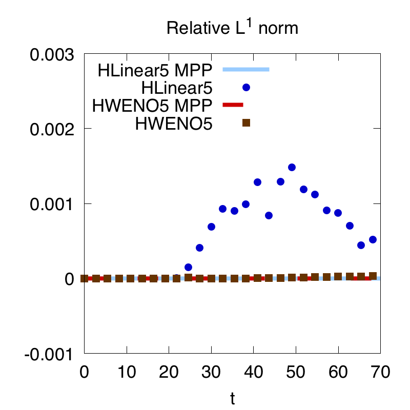
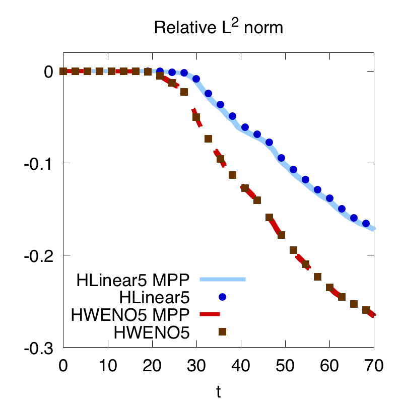
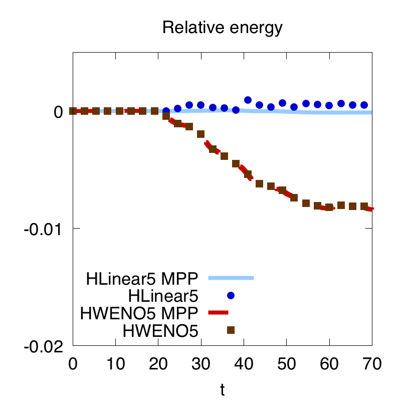
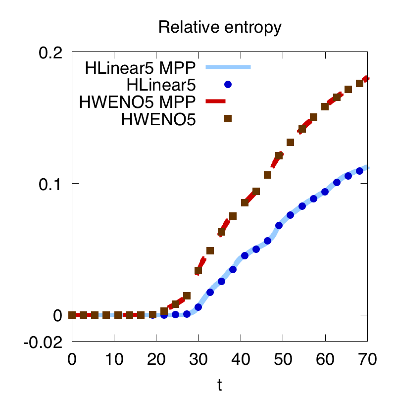
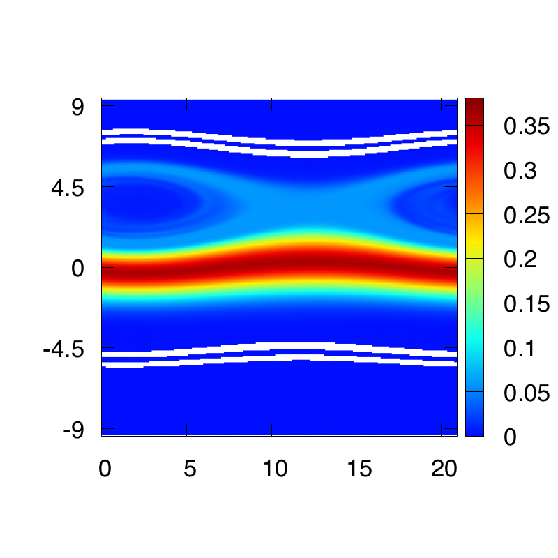
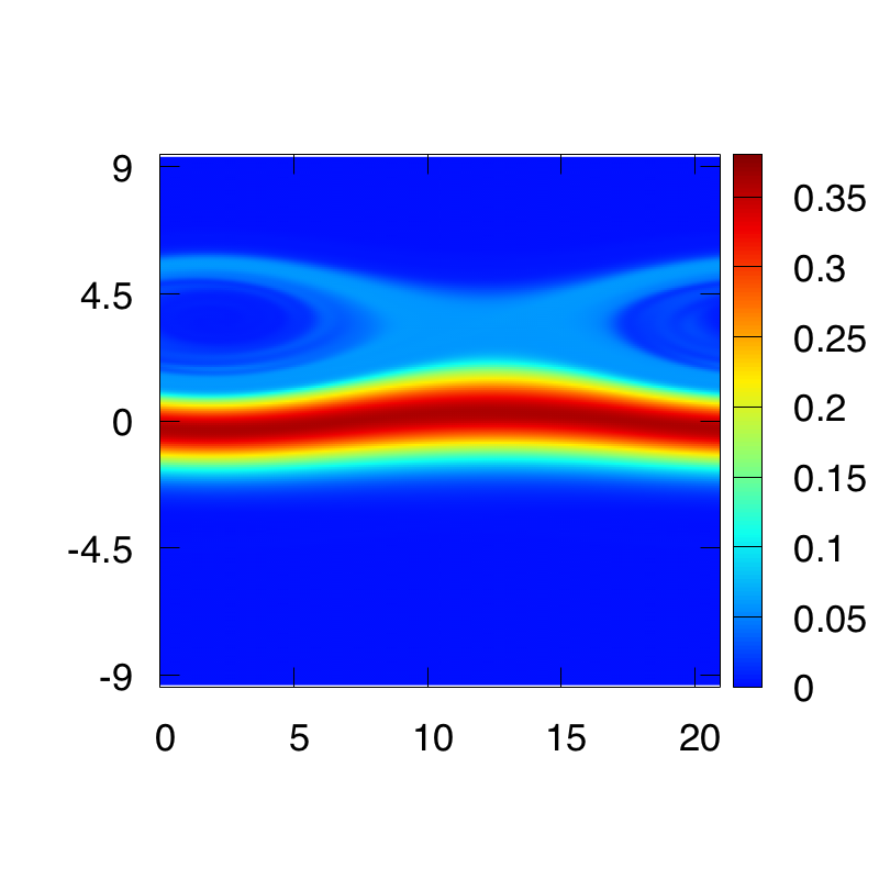
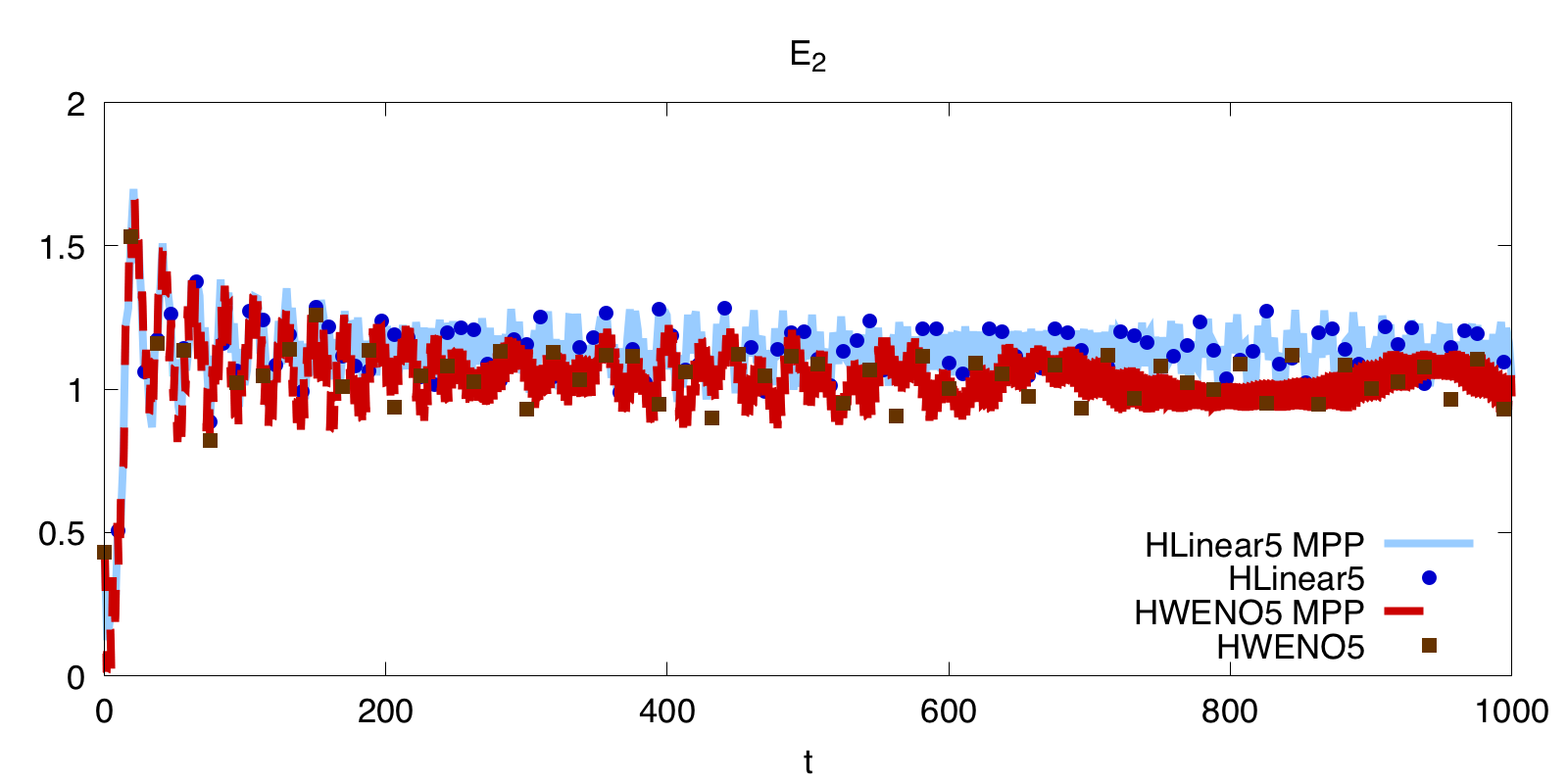
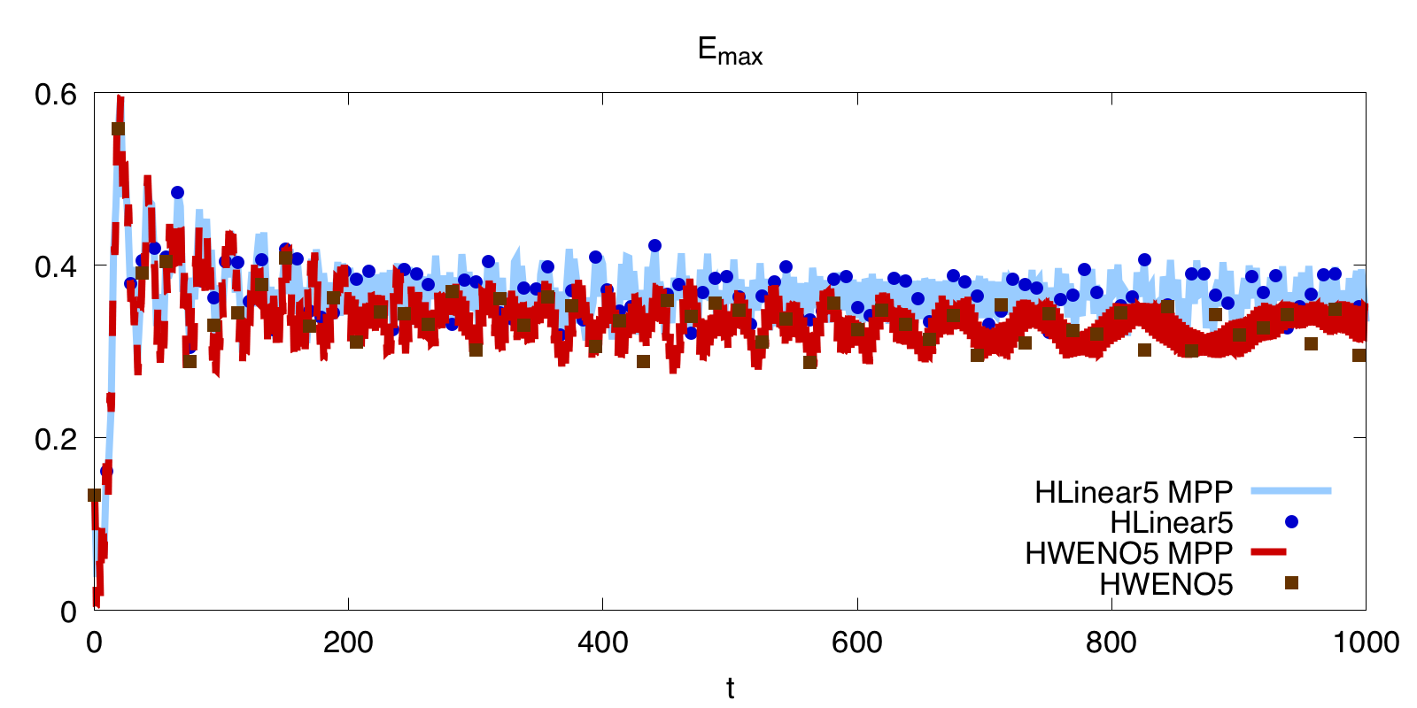
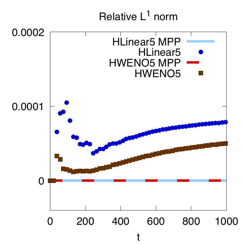
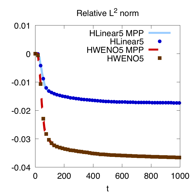
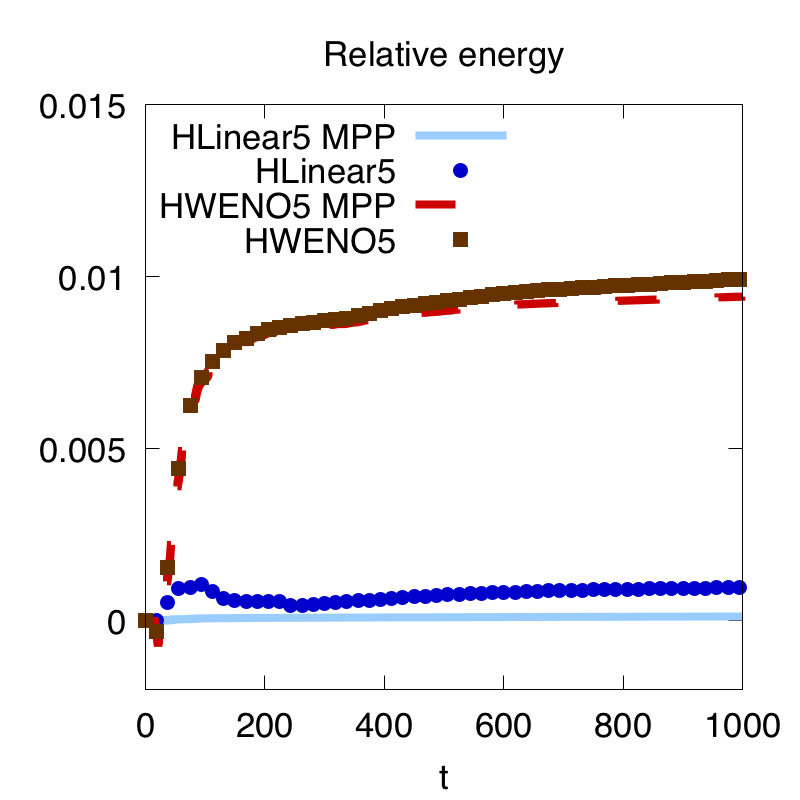
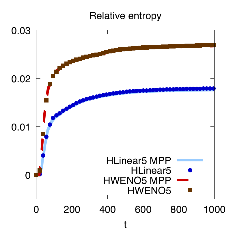
and , , , , , . The computational domain is . We take the cut-off domain in a little larger for the consideration of the shifting in the velocity. For this problem, the minimum value of the initial data is taking and in (3.11) and (3.12), while the maximum value is taking and . We run a long time simulation up to , which is a good test to show the effectiveness of the linear scheme in preserving some important quantities and the saving of computational cost as compared to the WENO type scheme. We first show the surface of the distribution function at in Fig. 3.6, we can clearly observe without limiter, the solution has undershootings, while the scheme with limiter produces very good result. We show the time evolution of the electric field in norm and norm in Fig. 3.7, and compare the linear scheme with the WENO type scheme. The norm of the electric filed matches those in [33, 1]. However, we can see that the linear scheme preserves the electric field better than the WENO type scheme after some large time, e.g., , while the results are almost the same between with and without limiter. We then show the relative derivation of the discrete norm, norm, kinetic energy and entropy in Fig. 3.8. The MPP limiter almost does not affect the norm and entropy, however, again we can see it improves the norm and the energy a lot from eliminating negative numerical values, which indicates the great performance of the MPP limiter on the linear scheme. Besides, the linear scheme preserves the norm, entropy and energy much better than the WENO type scheme, especially the energy. Moreover, for the computational cost, the linear scheme is at least about 3-4 times faster than the WENO type scheme. This example with long time simulation clearly demonstrates that the linear scheme is better than the WENO type scheme, which is much less dissipative and computationally much more efficient.
3.3. Kelvin-Helmholtz instability
Example 3.6.
The Kelvin-Helmholtz instability comes from the 2D guiding-center model (1.4) [16] with the initial data
| (3.13) |
and periodic boundary conditions on the domain . We let , which will create a Kelvin-Helmholtz instability. The exact solution should be within the range .
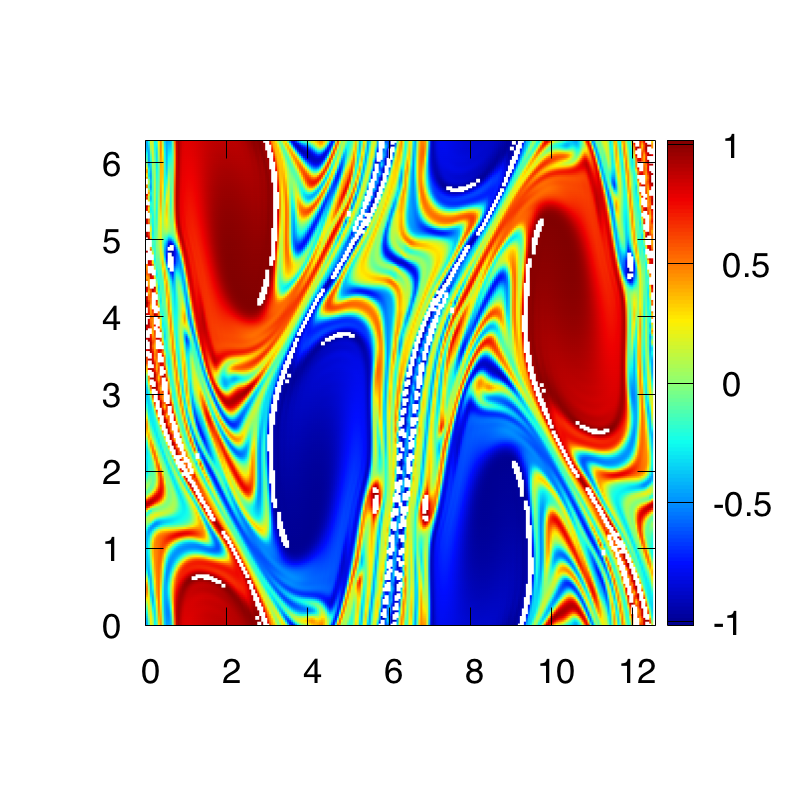
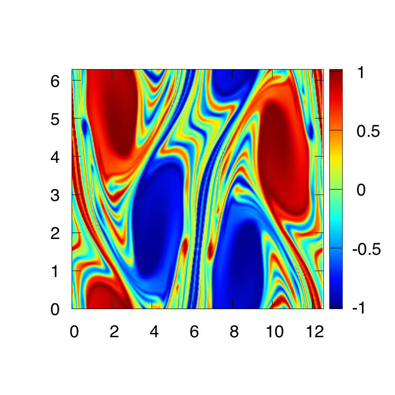
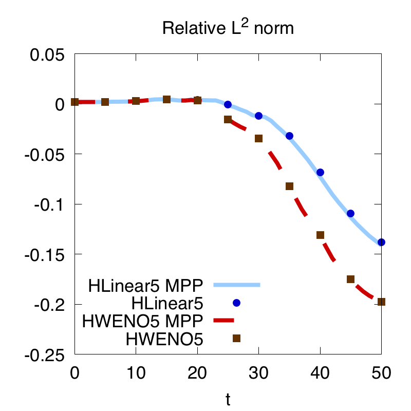
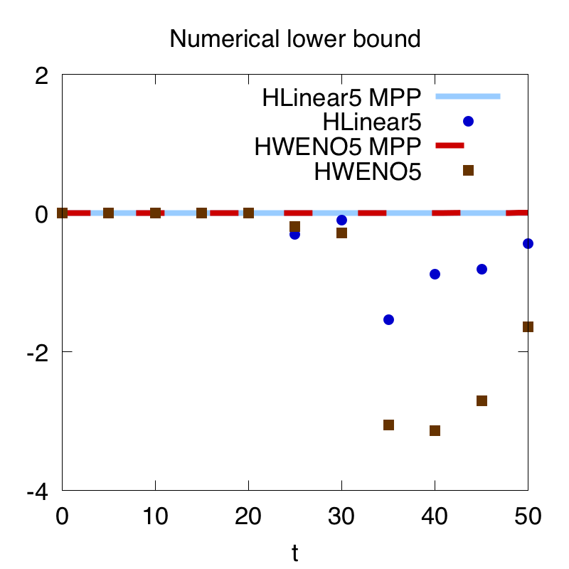
For this example, we show the solution at with mesh grid for “HLinear5” and “HLinear5 MPP” in Fig. 3.9 respectively. For the figures drawing in the physical range , we can observe white spots for “HLinear5” which is without MPP limiter, while “HLinear5 MPP” with MPP limiter preserves the bounds very well. In Fig. 3.10, we compare the time evolution of the relative norm and the numerical minimum values for both linear and WENO type schemes without and with limiters respectively. First, we can find that the linear scheme is less dissipative than the WENO one, as the norm preserves better for the linear scheme. The schemes with and without MPP limiter preserves the norm almost the same, so that there is no significant affection from the MPP limiter. For the minimum numerical values, the linear scheme without MPP limiter has shown large undershootings, the WENO type scheme without MPP limiter performs even worse for this example (which is also similar for the classic WENO scheme “WENO5”, we omit the figure here), but both schemes with MPP limiter preserve the lower bound very well. Similarly for the upper bound.
From this example, we can see that for problems with highly oscillatory but without discontinuous solutions, a high order linear scheme with the MPP limiter can result in a very good scheme, which is less dissipative and without significant spurious oscillations. The original idea to apply WENO reconstruction to suppress numerical oscillations seems to be even fail for this example. We can take this example as a benchmark test to support our main idea in this paper.
3.4. Incompressible Euler equations
Example 3.7.
(Accuracy test) We first consider the incompressible Euler system on the domain with an initial condition . The exact solution will stay stationary with , which is in the range of . For this example, from Table 3.3, we can see that the numerical solution with and without the limiter all stay in the right range, which shows that the limiter does not destroy the high order accuracy.
| N | error | order | error | order | |||
| WO | 32 | 2.34e-05 | – | 4.89e-05 | – | 2 | -2 |
| 64 | 8.86e-07 | 4.72 | 1.63e-06 | 4.91 | 2 | -2 | |
| 128 | 2.93e-08 | 4.92 | 5.08e-08 | 5.00 | 2 | -2 | |
| 256 | 9.43e-10 | 4.96 | 1.60e-09 | 4.99 | 2 | -2 | |
| WL | 32 | 2.34e-05 | – | 4.89e-05 | – | 2 | -2 |
| 64 | 8.86e-07 | 4.72 | 1.63e-06 | 4.91 | 2 | -2 | |
| 128 | 2.93e-08 | 4.92 | 5.08e-08 | 5.00 | 2 | -2 | |
| 256 | 9.43e-10 | 4.96 | 1.60e-09 | 4.99 | 2 | -2 |
Example 3.8.
(Vortex patch). In this example, we consider the incompressible Euler equations for the vortex patch problem with the initial condition given by
| (3.14) |
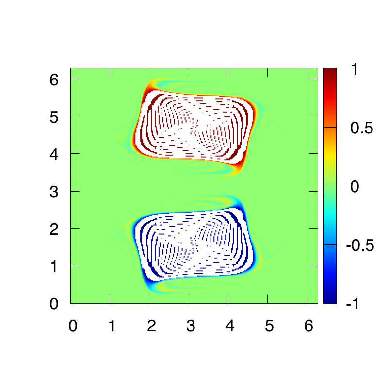
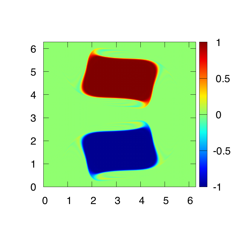
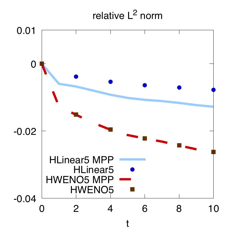
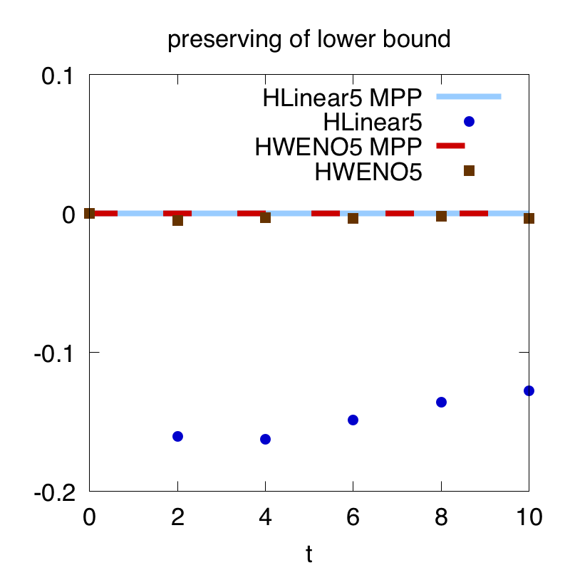
We show the surface of at in Fig. 3.11. The mesh grid is . We can observe the good performance of the MPP flux limiter on this problem. We also show the time evolution of the relative difference of norm as compared to the initial data, and the minimum numerical solution on the bottom of Fig. 3.11. Here we can still see that the linear scheme preserves the norm better than the WENO type scheme and the MPP limiter can eliminate the oscillations around two extreme values and from the schemes without limiter. However, we would mention that for this example with discontinuous initial data, the MPP limiter cannot remove the small numerical oscillations around (figures are omitted here). In this case, the WENO will be needed to completely remove oscillations for middle discontinuities.
4. Conclusion
In this paper, we have proposed a linear scheme combined with a high order bound-preserving MPP flux limiter, for solving incompressible flow problems. As compared to WENO type schemes, our approach is less dissipative and much less costly, so that is much more efficient for high dimensional problems with long time simulations. Applications to the Vlasov-Poisson system, 2D guiding-center model in plasma physics, as well as the incompressible Euler equations in fluid hydrodynamics have demonstrated the good performance of our proposed approach.
Acknowledgement
T. Xiong would like to thank Dr. F. Filbet for many helpful discussions. T. Xiong acknowledges support from the Marie Skłodowska-Curie Individual Fellowships H2020-MSCA-IF-2014 of the European Commission, under the project HNSKMAP 654175. This work has also been supported by the Fundamental Research Funds for the Central Universities No. 20720160009, NSFC grant 11601455, NSAF grant U1630247 and NSF grant of Fujian Province 2016J05022.
References
- [1] T. Arber and R. Vann, A critical comparison of Eulerian-grid-based Vlasov solvers, Journal of Computational Physics, 180 (2002), pp. 339–357.
- [2] B. Ayuso de Dios, J. A. Carrillo de la Plata, and C.-W. Shu, Discontinuous Galerkin methods for the one-dimensional Vlasov-Poisson system, Kinetic and Related Models, 4 (2011), pp. 955–989.
- [3] N. Besse, E. Deriaz, and É. Madaule, Adaptive multiresolution semi-Lagrangian discontinuous Galerkin methods for the Vlasov equations, Journal of Computational Physics, 332 (2017), pp. 376–417.
- [4] N. Besse and E. Sonnendrücker, Semi-Lagrangian schemes for the Vlasov equation on an unstructured mesh of phase space, Journal of Computational Physics, 191 (2003), pp. 341–376.
- [5] X. Cai, J. Qiu, and J.-M. Qiu, A conservative semi-Lagrangian HWENO method for the Vlasov equation, Journal of Computational Physics, 323 (2016), pp. 95–114.
- [6] J. A. Carrillo and F. Vecil, Nonoscillatory interpolation methods applied to Vlasov-based models, SIAM Journal on Scientific Computing, 29 (2007), pp. 1179–1206.
- [7] Y. Cheng, I. M. Gamba, and P. J. Morrison, Study of conservation and recurrence of Runge–Kutta discontinuous Galerkin schemes for Vlasov–Poisson systems, Journal of Scientific Computing, 56 (2013), pp. 319–349.
- [8] A. Christlieb, W. Guo, and Y. Jiang, A WENO-based method of lines transpose approach for Vlasov simulations, Journal of Computational Physics, 327 (2016), pp. 337–367.
- [9] N. Crouseilles, M. Mehrenberger, and E. Sonnendrücker, Conservative semi-Lagrangian schemes for Vlasov equations, Journal of Computational Physics, 229 (2010), pp. 1927–1953.
- [10] N. Crouseilles, M. Mehrenberger, and F. Vecil, Discontinuous Galerkin semi-Lagrangian method for Vlasov-Poisson, in ESAIM: Proceedings, vol. 32, EDP Sciences, 2011, pp. 211–230.
- [11] B. A. De Dios, J. A. Carrillo, and C.-W. Shu, Discontinuous Galerkin methods for the multi-dimensional Vlasov–Poisson problem, Mathematical Models and Methods in Applied Sciences, 22 (2012), p. 1250042.
- [12] W.-S. Don, Z. Gao, P. Li, and X. Wen, Hybrid compact-WENO finite difference scheme with conjugate Fourier shock detection algorithm for hyperbolic conservation laws, SIAM Journal on Scientific Computing, 38 (2016), pp. A691–A711.
- [13] E. Fijalkow, A numerical solution to the Vlasov equation, Computer Physics Communications, 116 (1999), pp. 319–328.
- [14] F. Filbet and E. Sonnendrücker, Comparison of Eulerian Vlasov solvers, Computer Physics Communications, 150 (2003), pp. 247–266.
- [15] F. Filbet, E. Sonnendrücker, and P. Bertrand, Conservative numerical schemes for the Vlasov equation, Journal of Computational Physics, 172 (2001), pp. 166–187.
- [16] E. Frénod, S. A. Hirstoaga, M. Lutz, and E. Sonnendrücker, Long time behaviour of an exponential integrator for a Vlasov-Poisson system with strong magnetic field, Communications in Computational Physics, 18 (2015), pp. 263–296.
- [17] W. Guo and Y. Cheng, An Adaptive Multiresoluton Discontinuous Galerkin Method for Time-Dependent Transport Equations in Multi-dimensions, arXiv preprint arXiv:1607.01822, (2016).
- [18] W. Guo and J.-M. Qiu, Hybrid semi-Lagrangian finite element-finite difference methods for the Vlasov equation, Journal of Computational Physics, 234 (2013), pp. 108–132.
- [19] R. E. Heath, I. M. Gamba, P. J. Morrison, and C. Michler, A discontinuous Galerkin method for the Vlasov–Poisson system, Journal of Computational Physics, 231 (2012), pp. 1140–1174.
- [20] F. Jia, Z. Gao, and W. S. Don, A spectral study on the dissipation and dispersion of the WENO schemes, Journal of Scientific Computing, 63 (2015), pp. 49–77.
- [21] C. Liang and Z. Xu, Parametrized maximum principle preserving flux limiters for high order schemes solving multi-dimensional scalar hyperbolic conservation laws, Journal of Scientific Computing, 58 (2014), pp. 41–60.
- [22] E. Madaule, S. A. Hirstoaga, M. Mehrenberger, and J. Pétri, Semi-Lagrangian simulations of the diocotron instability, Research Report, hal-00841504, (2013).
- [23] É. Madaule, M. Restelli, and E. Sonnendrücker, Energy conserving discontinuous Galerkin spectral element method for the Vlasov–Poisson system, Journal of Computational Physics, 279 (2014), pp. 261–288.
- [24] J.-M. Qiu and A. Christlieb, A conservative high order semi-Lagrangian WENO method for the Vlasov equation, Journal of Computational Physics, 229 (2010), pp. 1130–1149.
- [25] J.-M. Qiu and G. Russo, A High Order Multi-Dimensional Characteristic Tracing Strategy for the Vlasov–Poisson System, Journal of Scientific Computing, (2016), pp. 1–21.
- [26] J.-M. Qiu and C.-W. Shu, Conservative semi-Lagrangian finite difference WENO formulations with applications to the Vlasov equation, Communications in Computational Physics, 10 (2011), pp. 979–1000.
- [27] , Positivity preserving semi-Lagrangian discontinuous Galerkin formulation: theoretical analysis and application to the Vlasov–Poisson system, Journal of Computational Physics, 230 (2011), pp. 8386–8409.
- [28] J. A. Rossmanith and D. C. Seal, A positivity-preserving high-order semi-Lagrangian discontinuous Galerkin scheme for the Vlasov–Poisson equations, Journal of Computational Physics, 230 (2011), pp. 6203–6232.
- [29] C.-W. Shu, Essentially non-oscillatory and weighted essentially non-oscillatory schemes for hyperbolic conservation laws, in Advanced Numerical Approximation of Nonlinear Hyperbolic Equations, Springer, 1998, pp. 325–432.
- [30] C.-W. Shu and S. Osher, Efficient implementation of essentially non-oscillatory shock-capturing schemes, Journal of Computational Physics, 77 (1988), pp. 439–471.
- [31] E. Sonnendrücker, J. Roche, P. Bertrand, and A. Ghizzo, The semi-Lagrangian method for the numerical resolution of the Vlasov equation, Journal of Computational Physics, 149 (1999), pp. 201–220.
- [32] T. Xiong, J.-M. Qiu, and Z. Xu, A parametrized maximum principle preserving flux limiter for finite difference RK-WENO schemes with applications in incompressible flows, Journal of Computational Physics, 252 (2013), pp. 310–331.
- [33] T. Xiong, J.-M. Qiu, Z. Xu, and A. Christlieb, High order maximum principle preserving semi-Lagrangian finite difference WENO schemes for the Vlasov equation, Journal of Computational Physics, 273 (2014), pp. 618–639.
- [34] T. Xiong, G. Russo, and J.-M. Qiu, Conservative multi-dimensional semi-Lagrangian finite difference scheme: stability and applications to the kinetic and fluid simulations, arXiv preprint arXiv:1607.07409, (2016).
- [35] Z. Xu, Parametrized maximum principle preserving flux limiters for high order schemes solving hyperbolic conservation laws: one-dimensional scalar problem, Mathematics of Computation, 83 (2014), pp. 2213–2238.
- [36] Z. Xu and X. Zhang, Bound-preserving high-order schemes, in Handbook of Numerical Analysis, vol. 18, 2017, pp. 81–102.
- [37] C. Yang and F. Filbet, Conservative and non-conservative methods based on Hermite weighted essentially non-oscillatory reconstruction for Vlasov equations, Journal of Computational Physics, 279 (2014), pp. 18–36.
- [38] S. Zaki, T. Boyd, and L. Gardner, A finite element code for the simulation of one-dimensional Vlasov plasmas. II. Applications, Journal of Computational Physics, 79 (1988), pp. 200–208.
- [39] S. Zaki, L. Gardner, and T. Boyd, A finite element code for the simulation of one-dimensional Vlasov plasmas. I. theory, Journal of Computational Physics, 79 (1988), pp. 184–199.
- [40] X. Zhang, Y. Xia, and C.-W. Shu, Maximum-principle-satisfying and positivity-preserving high order discontinuous Galerkin schemes for conservation laws on triangular meshes, Journal of Scientific Computing, 50 (2012), pp. 29–62.
- [41] T. Zhou, Y. Guo, and C.-W. Shu, Numerical study on Landau damping, Physica D: Nonlinear Phenomena, 157 (2001), pp. 322–333.
- [42] H. Zhu, J. Qiu, and J.-M. Qiu, An h-Adaptive RKDG Method for the Vlasov–Poisson System, Journal of Scientific Computing, 69 (2016), pp. 1346–1365.
Tao Xiong
School of Mathematical Sciences,
Fujian Provincial Key Laboratory of Math. Mod. & HPSC,
Xiamen University, Xiamen, Fujian, P.R. China, 361005.
Université de Toulouse III
UMR5219, Institut de Mathématiques de Toulouse,
118, route de Narbonne
F-31062 Toulouse cedex, FRANCE
e-mail: txiong@xmu.edu.cn