Semi-discrete optimal transport — the case
Abstract
We consider the problem of finding an optimal transport plan between an absolutely continuous measure on and a finitely supported measure on when the transport cost is the Euclidean distance. We may think of this problem as closest distance allocation of some ressource continuously distributed over space to a finite number of processing sites with capacity constraints.
This article gives a detailed discussion of the problem, including a comparison with the much better studied case of squared Euclidean cost (“the case ”). We present an algorithm for computing the optimal transport plan, which is similar to the approach for by Aurenhammer, Hoffmann and Aronov [Algorithmica 20, 61–76, 1998] and Mérigot [Computer Graphics Forum 30, 1583–1592, 2011]. We show the necessary results to make the approach work for the Euclidean cost, evaluate its performance on a set of test cases, and give a number of applications. The later include goodness-of-fit partitions, a novel visual tool for assessing whether a finite sample is consistent with a posited probability density.
MSC 2010 Primary 65D18; Secondary 51N20, 62-09.
Key words and phrases: Monge–Kantorovich problem; spatial ressource allocation; Wasserstein metric; weighted Voronoi tesselation.
1 Introduction
Optimal transport and Wasserstein metrics are nowadays among the major tools for analyzing complex data. Theoretical advances in the last decades characterize existence, uniqueness, representation and smoothness properties of optimal transport plans in a variety of different settings. Recent algorithmic advances [36] make it possible to compute exact transport plans and Wasserstein distances between discrete measures on regular grids of tens of thousands of support points, see e.g. [42, Section 6], and to approximate such distances (to some extent) on larger and/or irregular structures, see [1] and references therein. The development of new methodology for data analysis based on optimal transport is a booming research topic in statistics and machine learning, see e.g. [50, 41, 3, 21, 18]. Applications are abundant throughout all of the applied sciences, including biomedical sciences (e.g. microscopy or tomography images [6, 22]), geography (e.g. remote sensing [13, 23]), and computer science (e.g. image processing and computer graphics [33, 48]). In brief: whenever data of a sufficiently complex structure that can be thought of as a mass distribution is available, optimal transport offers an effective, intuitively reasonable and robust tool for analysis.
More formally, for measures and on with the Wasserstein distance of order is defined as
| (1) |
where the minimum is taken over all transport plans (couplings) between and , i.e. measures on with marginals
for every Borel set . The minimum exists by [51, Theorem 4.1] and it is readily verified, see e.g. [51, after Example 6.3], that the map is a -valued metric on the space of measures with fixed finite mass. The constraint linear minimization problem (1) is known as Monge–Kantorovich problem [25, 51]. From an intuitive point of view, a minimizing describes how the mass of is to be associated with the mass of in order to make the overall transport cost minimal.
A transport map from to is a measurable map satisfying , where denotes the push-forward, i.e. for every Borel set . We say that induces the coupling if
for all Borel sets , and call the coupling deterministic in that case. It is easily seen that the support of is contained in the graph of . Intuitively speaking, we associate with each location in the domain of the measure exactly one location in the domain of the measure to which positive mass is moved, i.e. the mass of is not split.
The generally more difficult (non-linear) problem of finding (the -th root of)
| (2) |
where the infima are taken over all transport maps from to (and are in general not attained) is known as Monge’s problem [32, 51].
In practical applications, based on discrete measurement and/or storage procedures, we often face discrete measures and , where , are finite collections of support points, e.g. grids of pixel centers in a grayscale image. The Monge–Kantorovich problem (1) is then simply the discrete transport problem from classical linear programming [29]:
| (3) |
where and any measure is represented by the matrix with nonnegative entries satisfying
Due to the sheer size of and in typical applications this is still computationally a very challenging problem; we have e.g. for grayscale images, which is far beyond the performance of a standard transportation simplex or primal-dual algorithm. Recently many dedicated algorithms have been developed, such as [42], which can give enormous speed-ups mainly if and can compute exact solutions for discrete transportation problems with support points in seconds to a few minutes, but still cannot deal with or more points. Approximative solutions can be computed for this order of magnitude and by variants of the celebrated Sinkhorn algorithm [15, 43, 1], but it has been observed that these approximations have their limitations [43, 28].
The main advantage of using is that we can decompose the cost function as and hence formulate the Monge–Kantorovich problem equivalently as . For the discrete problem (3) this decomposition is used in [42] to construct particularly simple so-called shielding neighborhoods. But also if one or both of and are assumed absolutely continuous with respect to Lebesgue measure, this decomposition for has clear computational advantages. For example if the measures and are assumed to have densities and , respectively, the celebrated Brenier’s theorem, which yields an optimal transport map that is the gradient of a convex function [30], allows to solve Monge’s problem by finding a numerical solution to the Monge-Ampère equation ; see [40, Section 6.3] and the references given there.
In the rest of this article we focus on the semi-discrete setting, meaning here that the measure is absolutely continuous with respect to Lebesgue measure and the measure has finite support. This terminology was recently used in [52], [27], [20] and [10] among others. In the semi-discrete setting we can represent a solution to Monge’s problem as a partition of , where each cell is the pre-image of a support point of under the optimal transport map. We refer to such a partition as optimal transport partition.
In the case this setting is well studied. It was shown in [5] that an optimal transport partition always exists, is essentially unique, and takes the form of a Laguerre tessellation, a.k.a. power diagram. The authors proved further that the right tessellation can be found numerically by solving a (typically high dimensional) unconstrained convex optimization problem. Since Laguerre tessellations are composed of convex polytopes, the evaluation of the objective function can be done very precisely and efficiently. [31] elaborates details of this algorithm and combines it with a powerful multiscale idea. In [27] a damped Newton algorithm is presented for the same objective function and the authors are able to show convergence with optimal rates.
In this article we present the corresponding theory for the case . It is known from [19], which treats much more general cost functions, that an optimal transport partition always exists, is essentially unique and takes the form of a weighted Voronoi tessellation, or more precisely an Apollonius diagram. We extend this result somewhat within the case in Theorems 1 and 2 below. We prove then in Theorem 3 that the right tessellation can be found by optimizing an objective function corresponding to that from the case . Since the cell boundaries in an Apollonius diagram in 2d are segments of hyperbolas, computations are more involved and we use a new strategy for computing integrals over cells and for performing line search in the optimization method. Details of the algorithm are given in Section 4 and the complete implementation can be downloaded from Github222https://github.com/valentin-hartmann-research/semi-discrete-transport and will be included in the next version of the transport-package [46] for the statistical computing environment R [38]. Up to Section 4 the present paper is a condensed version of the thesis [24], to which we refer from time to time for more details. In the remainder we evaluate the performance of our algorithm on a set of test cases (Section 5), give a number of applications (Section 6), and provide a discussion and open questions for further research (Section 7).
At the time of finishing the present paper, it has come to our attention that Theorem 2.1 of [27], which is for very general cost funtions including the Euclidean distance (although the remainder of the paper is not), has a rather large overlap with our Theorem 3. Within the case of Euclidean cost it assumes somewhat stronger conditons than our Theorem 3, namely a compact domain and a bounded density for . In addition the statement is somewhat weaker as it does not contain our statement (c). We also believe that due to the simpler setting of our proof is accessible to a wider audience and it is more clearly visible that the additional restrictions on and are in fact not needed.
We end this introduction by providing some first motivation for studying the semi-discrete setting for . This will be further substantiated in the application section 6.
1.1 Why semi-discrete?
The semi-discrete setting appears naturally in problems of allocating a continuously distributed resource to a finite number of sites. Suppose for example that a fast-food chain introduces a home delivery service. Based on a density map of expected orders (the “resource”), the management would like to establish delivery zones for each branch (the “sites”). We assume that each branch has a fixed capacity (at least in the short run), that the overall capacity matches the total number of orders (peak time scenario), and that the branches are not too densely distributed, so that the Euclidean distance is actually a reasonable approximation to the actual travel distance; see [9]. We take up this example in Subsection 6.2.
An important problem that builds on resource allocation is the quantization problem: Where to position a number of sites in such a way that the resulting resource allocation cost is minimal? See [10, Section 4] for a recent discussion using incomplete transport and .
As a further application we propose in Subsection 6.3 optimal transport partitions as a simple visual tool for investigating local deviations from a continuous probability distribution based on a finite sample.
Since the computation of the semi-discrete optimal transport is linear in the resolution at which we consider the continuous measure (for computational purposes), it can also be attractive to use the semi-discrete setting as an approximation of either the fully continuous setting (if is sufficiently simple) or the fully discrete setting (if has a large number of support points). This will be further discussed in Section 2.
1.2 Why ?
The following discussion highlights some of the strengths of optimal transport based on an unsquared Euclidean distance (), especially in the semi-discrete setting, and contrasts with .
From a computational point of view the case can often be treated more efficiently, mainly due to the earlier mentioned decomposability, leading e.g. to the algorithms in [42] in the discrete and [5, 31] in the semi-discrete setting. The case has the advantage that the Monge–Kantorovich problem has a particularly simple dual [51, Particular Case 5.16], which is equivalent to Beckmann’s problem [7] [40, Theorem 4.6]. If we discretize the measures (if necessary) to a common mesh of points, the latter is an optimization problem in variables rather than the variables needed for the general discrete transport formulation (3). Algorithms that make use of this reduction have been described in [49] (for general discrete surfaces) and in [44, Section 4] (for general incomplete transport), but their performance in a standard situation, e.g. complete optimal transport on a regular grid in , remains unclear. In particular we are not aware of any performance comparisons between and .
In the present paper we do not make use of this reduction, but keep the source measure truly continuous except for an integral approximation that we perform for numerical purposes. We describe an algorithm for the semi-discrete problem with that is reasonably fast, but cannot quite reach the performance of the algorithm for in [31]. This is again mainly due to the nice decomposition property of the cost function for or, more blatantly, the fact that we minimize for over partitions formed by line rather than hyperbola segments.
From an intuitive point of view and have both nice interpretations and depending on the application setting either the one or the other may be more justified. The difference is between thinking in terms of transportation logistics or in terms of fluid mechanics. If the optimal transport plan minimizes the cumulative distance by which mass is transported. This is (up to a factor that would not change the transport plan) the natural cost in the absence of fixed costs or any other savings on long-distance transportation. If the optimal transport plan is determined by a pressureless potential flow from to as seen from the kinetic energy minimization formulation of Benamou and Brenier [8] [51, Chapter 7].
The different behaviors in the two cases can be illustrated by the discrete toy example in Figure 1. Each point along the incomplete circle denotes the location of one unit of mass of (blue x-points) and/or (red o-points). The unique solution for moves one unit of mass from one end of the circular structur to the other. This is how we would go about carrying boxes around to get from the blue scenario to the red scenario. The unique solution for on the other hand is to transport each unit a tiny bit further to the next one, corresponding to a (discretized) flow along the circle. It is straightforward to adapt this toy example for the semi-discrete or the continuous setting. A more complex semidiscrete example is given in Subsection 6.1.
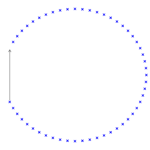
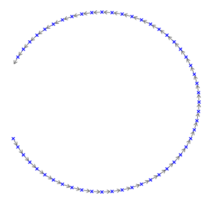
One argument in favour of the metric is its nice invariant properties that are not shared by the other . In particular, considering finite measures on satisfying , and , we have
| (4) | ||||
| (5) |
The first result is in general not true for any other , the second result holds with an additional factor on the right hand side. We prove these statements in the appendix. These invariance properties have important implications for image analysis, where it is quite common to adjust for differring levels of brightness (in greyscale images) by affine transformations. While the above equalities show that it is safe to do so for , it may change the resulting Wasserstein distance and the optimal transport plan dramatically for other ; see Appendix and Subsection 6.1.
It is sometimes considered problematic that optimal transport plans for are in general not unique. But this is not so in the semi-discrete case, as we will see in Section 2: The minimal transport cost in (1) is realized by a unique coupling , which is always deterministic. The same is true for . A major difference in the case is that for each cell of the optimal transport partition contains the support point of the target measure that it assigns its mass to. This can be seen as a consequence of cyclical monotonicity [51, beginning of Chapter 8]. In contrast, for , optimal transport cells can be separated by many other cells from their support points, which can make the resulting partition hard to interpret without drawing corresponding arrows for the assignment; see the bottom panels of Figure 5. For this reason we prefer to use for the goodness-of-fit partitions considered in Subsection 6.3.
2 Semi-discrete optimal transport
We first concretize the semi-discrete setting and introduce some additional notation. Let now and be Borel subsets of and let and be probability measures on and , respectively. This is just for notational convenience and does not change the set of admissible measures in an essential way: We may always set and any statement about and we make can be easily recovered for and for arbitrary .
For the rest of the article it is tacitly assumed that to avoid certain pathologies of the one-dimensional case that would lead to a somewhat tedious distinction of cases in various results for a case that is well-understood anyway. Moreover, we always require to be absolutely continuous with density with respect to -dimensional Lebesgue measure and to satisfy
| (6) |
We asssume further that , where , and . Condition (6) guarantees that
| (7) |
which simplifies certain arguments.
The set of Borel subsets of is denoted by . Lebesgue mass is denoted by absolute value bars, i.e. for every .
We call a partition of into Borel sets satisfying for every a transport partition from to . Any such partition characterizes a transport map from to , where we set for a given transport partition and for a given transport map . Monge’s problem for can then be equivalently formulated as finding
| (8) |
where the infima are taken over all transport partitions from to . Contrary to the difficulties encountered for more general measures and when considering Monge’s problem with Euclidean costs, we can give a clear-cut existence and uniqueness theorem in the semi-discrete case, without any further restrictions.
Theorem 1.
In the semi-discrete setting with Euclidean costs (always including and (6)) there is a -a.e. unique solution to Monge’s problem. The induced coupling is the unique solution to the Monge–Kantorovich problem, yielding
| (9) |
Proof.
The part concerning Monge’s problem is a consequence of the concrete construction in Section 3; see Theorem 2.
Clearly is an admissible transport plan for the Monge–Kantorovich problem. Since is non-atomic and the Euclidean cost function is continuous, Theorem B in [37] implies that the minimum in the Monge–Kantorovich problem is equal to the infimum in the Monge problem, so must be optimal.
For the uniqueness of in the Monge–Kantorovich problem, let be an arbitrary optimal transport plan. Define the measures on by for all and . Since , all are absolutely continuous with respect to with densities satisfying . Set then .
Assume first that there exist , , such that . Define and , analogously. There exists a for which both and have positive Lebesgue measure: Choose such that and ; using binary search between and , we find the desired in finitely many steps, because otherwise there would have to exist a such that , which is not possible. By the definition of and we thus have and . Switching and if necessary, we may assume . Define then
and for . It can be checked immediately that the measure given by for all and all is a transport plan from to again. It satisfies
because the integrands are strictly negative on the sets over which we integrate. But this contradicts the optimality of .
We thus have proved that for all pairs with . This implies that we can define a transport map inducing in the following way. If for some , set . Since the intersections are Lebesgue null sets, the value of on them does not matter. So we can for example set or for , where contains at least to elements and . It follows that . But by the optimality of and Theorem 2 we obtain -almost surely, which implies . ∎
It will be desirable to know in what way we may approximate the continuous and discrete Monge–Kantorovich problems by the semi-discrete problem we investigate here.
In the fully continuous case, we have a measure on with density with respect to instead of the discrete measure . In the fully discrete case, we have a discrete measure instead of the absolutely continuous measure , where , and . In both cases existence of an optimal transport plan is still guaranteed by [51, Theorem 4.1], however we lose to some extent the uniqueness property.
One reason for this is that mass transported within the same line segment can be reassigned at no extra cost; see the discussion on transport rays in Section 6 of [2]. In the continuous case this is the only reason, and uniqueness can be restored by minimizing a secondary functional (e.g. total cost with respect to ) over all optimal transport plans; see Theorem 7.2 in [2].
In the discrete case uniqueness depends strongly on the geometry of the support points of and . In addition to collinearity of support points, equality of interpoint distances can also lead to non-unique solutions. While uniqueness can typically be achieved when the support points are in sufficiently general position, we are not aware of any precise result to this effect.
When approximating the continuous problem with measures and by a semi-discrete problem, we quantize the measure to obtain a discrete measure , where for a partition of . The error we commit in Wasserstein distance by discretization of is bounded by the quantization error, i.e.
| (10) |
We can compute exactly by solving another semi-discrete transport problem, using the algorithm described in Section 4 to compute an optimal partition for the second inequality above. However, choosing for given in such a way that is minimal is usually practically infeasible. So we would use an algorithm that makes reasonably small, such as a suitable version of Lloyd’s algorithm; see Subsection 4.1 below.
When approximating the discrete problem with measures and by a semi-discrete problem, we blur each mass of over a neighborhood of using a probability density , to obtain a measure with density . Typical examples use , where is the standard normal density and the bandwidth is reasonably small, or , where is some small neighborhood of . In practice, discrete measures are often available in the form of images, where the support points form a fine rectangular grid; then the latter choice of s is very natural, where the s are just adjacent squares, each with an at the center. There are similar considerations for the approximation error as in the fully continuous case above. In particular the error we commit in Wasserstein distance is bounded by the blurring error
| (11) |
The right hand side is typically straightforward to compute exactly, e.g. in the normal density and grid cases described above. It can be made small by choosing the bandwidth very small or picking sets of small radius .
What about the approximation properties of the optimal transport plans obtained by the semi-discrete setting? Theorem 5.20 in [51] implies for weakly and weakly that every subsequence of the sequence of optimal transport plans between and has a further subsequence that converges weakly to an optimal transport plan between and . This implies that for every there is a such that for any the plan is within distance (in any fixed metrization of the weak topology) of some optimal transport plan between and , which is the best we could have hoped for in view of the non-uniqueness of optimal transport plans we have in general. If (in the discrete setting) there is a unique optimal transport plan , this yields that weakly.
3 Optimal transport maps via weighted Voronoi tessellations
As shown for bounded in [19], the solution to the semi-discrete transport problem has a nice geometrical interpretation, which is similar to the well-known result in [5]: We elaborate below that the sets of the optimal transport partition are the cells of an additively weighted Voronoi tessellation of around the support points of .
For the finite set of points and a vector that assigns to each a weight , the additively weighted Voronoi tessellation is the set of cells
Note that adjacent cells and have disjoint interiors. The intersection of their boundaries is a subset of , which is easily seen to have Lebesgue measure (and hence -measure) zero. If , the set is a branch of a hyperbola with foci at and . It may also be interpreted as the set of points that have the same distance from the spheres and , where . See Figure 2 for an illustration of these properties.
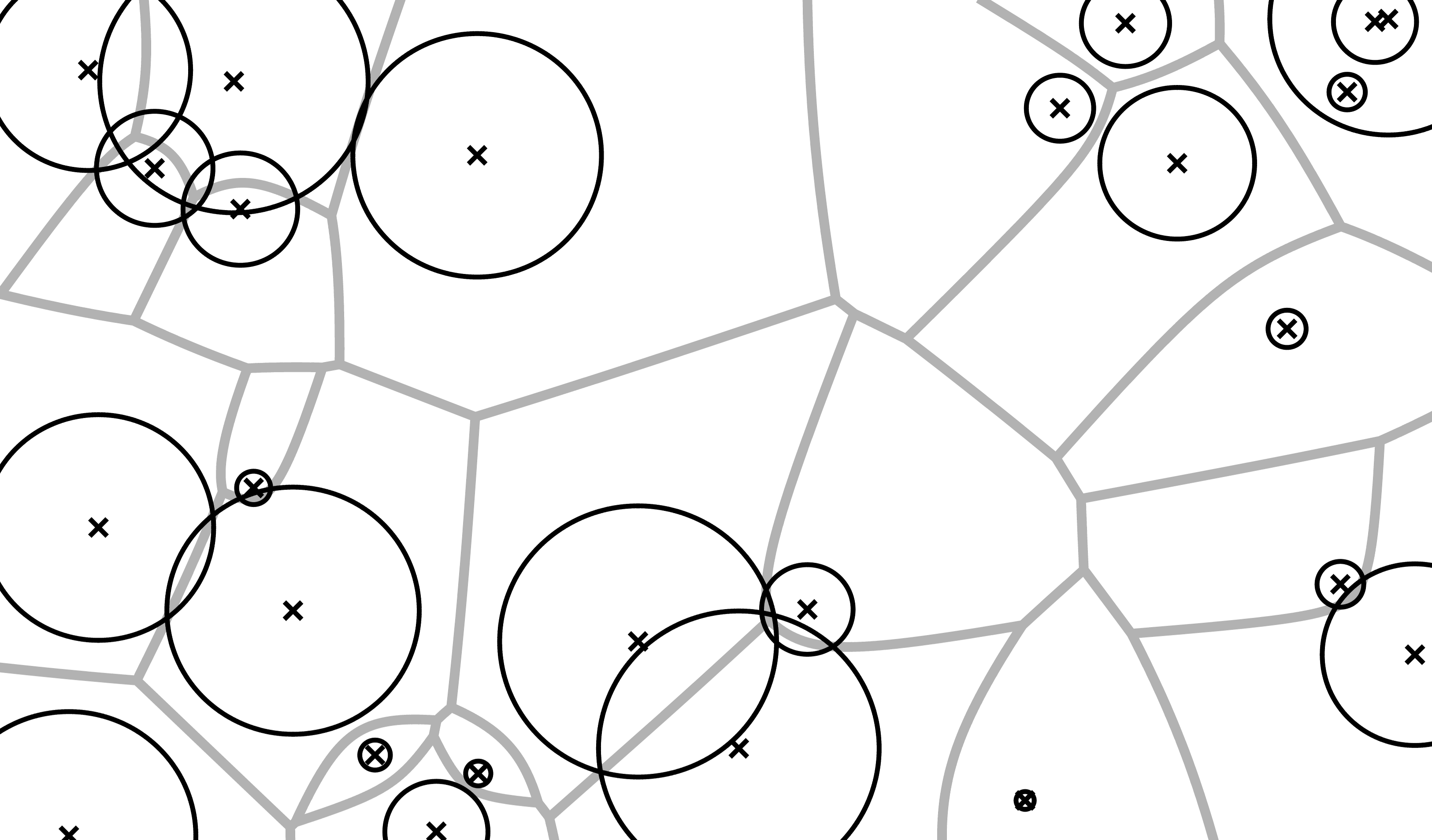
Of course not all weighted Voronoi tessellations are valid transport partitions from to . But suppose we can find a weight vector such that the resulting Voronoi tessellation satisfies indeed for every ; we call such a adapted to . Then this partition is automatically optimal.
Theorem 2.
If is adapted to , then is the -almost surely unique optimal transport partition from to .
A proof was given in [19, Theorem 2] for more general distance functions, but required to be bounded. For the Euclidean distance we consider here, we can easily extend it to unbounded ; see [24, Theorem 3.2].
Having identified this class of optimal transport partitions, it remains to show that for each pair we can find an adapted weight vector. We adapt the approach of [5] to the case , which gives us a constructive proof that forms the basis for the algorithm in Section 4. Our key tool is the function defined below.
Theorem 3.
Let ,
Then
-
a)
is convex;
-
b)
is continuously differentiable with partial derivatives
-
c)
takes a minimum in .
Remark 1.
of Theorem 3.
We take a few shortcuts; for full technical details see Chapter 3 of [24].
Part a) relies on the observation that can be written as
where
denotes the transport map induced by the Voronoi tessellation with weight vector and we write instead of for convenience. By definition of the weighted Voronoi tessellation is the infimum of the affine functions
over all measurable maps from to . Since pointwise infima of affine functions are concave and the first summand of is linear, we see that convex.
By geometric arguments it can be shown that is continuous; see [24, Lemma 3.3]. A short computation involving the representation used above yields for the difference quotient of , writing for the -th standard basis vector and letting ,
as . This implies that is with (continuous) -th partial derivative and hence statement b) follows.
Finally, for the existence of a minimizer of we consider an arbitrary sequence of weight vectors in with
We show below that a suitably shifted version of that has the same -values contains a bounded subsequence. This subsequence then has a further subsequence which converges towards some . Continuity of yields
and thus statement c).
To obtain the bounded subsequence, note first that adding to each weight the same constant neither affects the Voronoi tessellation nor the value of . We may therefore assume , , for all . Choosing an entry and an infinite set appropriately leaves us with a sequence satisfying for all and . Taking a further subsequence for some infinite allows the choice of an and the partitioning of into two sets and such that for every
-
i)
-
ii)
where denotes the rank of in .
Assume that . The Voronoi cells with indices in will at some point be shrunk to measure zero, meaning there exists an such that
Write
and recall the constant from (7), which may clearly serve as an upper bound for the transport cost under an arbitrary plan. We then obtain for every
which contradicts the statement . Thus we have .
We can then simply turn into a bounded sequence by substracting the minimal entry from each for all . ∎
4 The algorithm
The previous section provides the theory needed to compute the optimal transport partition. It is sufficient to find a vector where is locally optimal. By convexity, is then a global minimizer of and Remark 1 identifies the -a.e. unique optimal transport partition as .
For the optimization process we can choose from a variety of methods thanks to knowing the gradient of analytically from Theorem 3. We consider iterative methods that start at an initial weight vector and apply steps of the form
where denotes the search direction and the step size.
Newton’s method would use , but the Hessian matrix is not available to us. We therefore use a quasi-Newton method that makes use of the gradient. Just like [31] for the case , we have obtained many good results using L-BFGS [34], the limited-memory variant of the Broyden–Fletcher–Goldfarb–Shanno algorithm, which uses the value of the gradient at the current as well as at preceding steps for approximating the Hessian. The limited-memory variant works without storing the whole Hessian of size , which is important since in applications our is typically large.
To determine a suitable step size we use the Armijo rule [4], which has proven to be well suited for our problem. It considers different values for until it arrives at one that sufficiently decreases . We also considered replacing the Armijo rule with the strong Wolfe conditions [53, 54] as done in [31], which contain an additional decrease requirement on the gradient. In our case, however, this requirement could often not be fulfilled because of the pixel splitting method used for computing the gradient (cf. Sec. 4.2), which made it less suited.
4.1 Multiscale approach to determine starting value
To find a good starting value we use a multiscale method similar to the one proposed in [31]. We first create a decomposition of , i.e. a sequence of measures with decreasing cardinality of the support. Here is obtained as a coarsening of by merging the masses of several points into one point.
It seems intuitively reasonable to choose in such a way that is as small as possible, since the latter bounds . This comes down to a capacitated location-allocation problem, which is NP-hard even in the one-dimensional case; see [47]. Out of speed concerns and since we only need a reasonably good starting value for our algorithm, we decided to content ourselves with the same weighted -means clustering algorithm used by [31] (referred to as Lloyd’s algorithm), which iteratively improves an initial aggregation of the support of into clusters towards local optimality with respect to the squared Euclidean distance. The resulting is then the discrete measure with the cluster centers as its support points and as weights the summed up weights of the points of contained in each cluster; see Algorithm 3 in [24]. The corresponding weighted -median clustering algorithm, based on alternating between assignment of points to clusters and recomputation of cluster centers as the median of all weighted points in the cluster, should intuitively give a based on which we obtain a better starting solution. This may sometimes compensate for the much longer time needed for performing -median clustering.
Having created the decomposition , we minimize along the sequence of these coarsened measures, beginning at with the initial weight vector and computing the optimal weight vector for the transport from to . Every time we pass to a finer measure from the coarser measure , we generate the initial weight vector from the last optimal weight vector by assigning the weight of each support point of to all the support points of from whose merging the point of originated; see also Algorithm 2 in [24].
4.2 Numerical computation of and
For practical computation we assume here that is a bounded rectangle in and that the density of the measure is of the form
for , where we assume that is a finite index set and is a partition of the domain into (small) squares, called pixels, of equal side length. This is natural if is given as a grayscale image and we would then typically index the pixels by their centers . It may also serve as an approximation for arbitrary . It is however easy enough to adapt the following considerations to more general (not necessarily congruent) tiles and to obtain better approximations if the function is specified more generally than piecewise constant.
The optimization procedure requires the non-trivial evaluation of at a given weight vector . This includes the integration over Voronoi cells and therefore the construction of a weighted Voronoi diagram. The latter task is solved by the package 2D Apollonius Graphs as part of the Computational Geometry Algorithms Library [11]. The integrals we need to compute are
By definition the boundary of a Voronoi cell is made up of hyperbola segments, each between and one of the other support points of . The integration could be performed by drawing lines from to the end points of those segments and integrating over the resulting triangle-shaped areas separately. This would be executed by applying an affinely-linear transformation that moves the hyperbola segment onto the hyperbola to both the area and the function we want to integrate. The required transformation can be found in [24, Section 5.6].
However, we take a somewhat more crude, but also more efficient path here, because it is a quite time-consuming task to decide which pixels intersect which weighted Voronoi cells and then to compute the (areas of the) intersections. We therefore approximate the intersections by splitting the pixels into a quadratic number of subpixels (unless the former are already very small) and assuming that each of them is completely contained in the Voronoi cell in which its center lies. This reduces the problem from computing intersections to determining the corresponding cell for each center, which the data structure used for storing the Voronoi diagram enables us to do in roughly time; see [26]. The operation can be performed even more efficiently: When considering a subpixel other than the very first one, we already know the cell that one of the neighboring subpixel’s center belongs to. Hence, we can begin our search at this cell, which is either already the cell we are looking for or lies very close to it.
The downside of this approximation is that it can make the L-BFGS algorithm follow search directions along which the value of cannot be sufficiently decreased even though there exist different directions that allow a decrease. This usually only happens near a minimizing weight vector and can therefore be controlled by choosing a not too strict stopping criterion for a given subpixel resolution, see the next subsection.
4.3 Our implementation
Implementing the algorithm described in this section requires two technical choices: The number of subpixels every pixel is being split into and the stopping criterion for the minimization of . We found that choosing the number of subpixels to be the smallest square number such that their total number is larger than or equal to gives a good compromise between performance and precision.
The stopping criterion is implemented as follows: We terminate the optimization process once for some . Due to Theorem 3b) this criterion yields an intuitive interpretation: is the amount of mass that is being mistransported, i.e. the total amount of mass missing or being in surplus at some -location when transporting according to the current tessellation. In our experience this mass is typically rather proportionally distributed among the different cells and tends to be assigned in a close neighbourhood of the correct cell rather than far away. So even with somewhat larger , the computed Wasserstein distance and the overall visual impression of the optimal transport partition remain mostly the same. In the numerical examples in Sections 5 and 6 we choose the value of .
We implemented the algorithm in C++ and make it available on GitHub333https://github.com/valentin-hartmann-research/semi-discrete-transport under the MIT license. Our implementation uses libLBFGS [35] for the L-BFGS procedure and the geometry library CGAL [11] for the construction and querying of weighted Voronoi tessellations. The repository also contains a Matlab script to visualize such tessellations. Our implementation will also be included in a future version of the transport-package [46] for the statistical computing environment R [38].
5 Performance evaluation
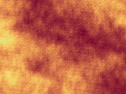
We evaluated the performance of our algorithm by randomly generating measures and with varying features and computing the optimal transport partitions between them. The measure was generated by simulating its density as a Gaussian random field with Matérn covariance function on the rectangle , applying a quadratic function and normalizing the result to a probability density. Corresponding images were produced at resolution pixels and were further divided into 25 subpixels each to compute integrals over Voronoi cells. In addition to a variance parameter, which we kept fixed, the Matérn covariance function has parameters for the scale of the correlations, which we varied among , and , and the smoothness of the generated surface, which we varied between and corresponding to a continuous surface and a -surface, respectively. The simulation mechanism is similar to the ones for classes 2–5 in the benchmark DOTmark proposed in [45], but allows to investigate the influence of individual parameters more directly. Figure 3 shows one realization for each parameter combination. For the performance evaluation we generated 10 realizations each.
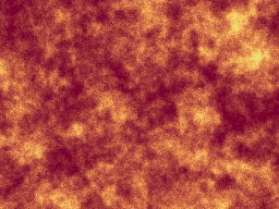



The measures have support points generated uniformly at random on , where we used and . We then assigned either mass or mass to each point and normalized to obtain probability measures. We generated 20 independent -measures of the first kind (unit mass) and computed the optimal transport from each of the -measures for each of the 6 parameter combinations. We further generated for each of the -measures corresponding -measure of the second kind (masses from ) and computed again the corresponding optimal transports. The stopping criterion for the optimization was an amount of of mistransported mass.
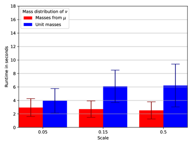
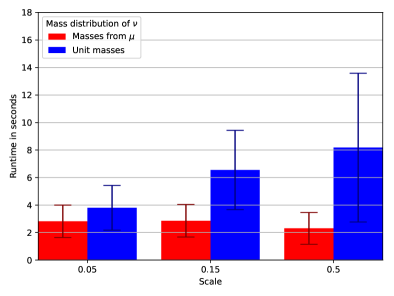
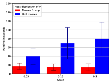
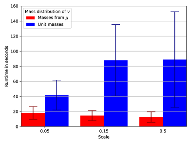
The results for support points of are shown in Figures 4(a) and 4(b), those for support points in Figures 4(c) and 4(d). Each bar shows the mean of the runtimes on one core of a mobile Intel Core i7 across the 200 experiments for the respective parameter combination; the blue bars are for the measures with uniform masses, the red bars for the measures with masses selected from the corresponding measure. The lines indicate the standard deviations.
We observe that computation times stay more or less the same between parameter choices (with some sampling variation) if the -masses are taken from the corresponding -measure. In this case mass can typically be assigned (very) locally, and slightly more so if has fewer local fluctuations (higher and/or ). This seems a plausible explanation for the relatively small computation times.
In contrast, if all -masses are the same, the computation times are considerably higher and increase substantially with increasing and somewhat with increasing smoothness. This seems consistent with the hypothesis that the more the optimal transport problem can be solved by assigning mass locally the lower the computation times. For larger scales many of the support points of compete strongly for the assignment of mass and a solution can only be found globally. A lower smoothness may alleviate the problem somewhat, because it creates locally more variation in the available mass.
We would like to note that to the best of our knowledge the present implementation is the first one for computing the optimal transport in the semi-discrete setting for the case , which means that fair performance comparisons with other algorithms are not easily possible.
6 Applications
We investigate three concrete problem settings in order to better understand the workings and performance of our algorithm as well as to illustrate various theoretical and practical aspects pointed out in the paper.
6.1 Optimal transport between two normal distributions
We consider two bivariate normal distributions and , where , and , i.e. they both have the same spherical covariance matrix such that one distribution is just a displacement of the other. For computations we have truncated both measures to the set . By discretization (quantization) a measure is obtained from . We then compute the optimal transport partition and the Wasserstein distances between and for both and . Computations and plots for are obtained with the package transport [46] for the statistical computing environment R [38]. For we use our implementation presented in the previous section.
Note that for the original problem of optimal transport from to the solution is known exactly, so we can use this example to investigate the correct working of our implementation. In fact, for any probability measure on and its displacement , where for some vector , it is immediately clear that the translation induces an optimal transport plan for (1) and that for arbitrary . This holds because we obtain by Jensen’s inequality for , ; therefore and is clearly a transport map from to that achieves this lower bound. For Theorem 9.4 in [51] yields that is the unique optimal transport map and the induced plan is the unique optimal transport plan. In the case neither of these objects is unique due to the possibility to rearrange mass transported within the same line segment at no extra cost.
Discretization was performed by applying the weighted -means algorithm based on the discretization of to a fine grid and an initial configuration of cluster centers drawn independently from distribution and equipped with the corresponding density values of as weights. The number of cluster centers was kept to for better visibility in the plots below. We write for the discretized measure. The discretization error can be computed numerically by solving another semi-discrete transport problem, see the third column of Table 1 below.
The first column of Figure 5 depicts the measures and and the resulting optimal transport partitions for and . In the case the nuclei of the weighted Voronoi tessellation are always contained in their cells, whereas for this need not be the case. We therefore indicate the relation by a gray arrow pointing from the centroid of the cell to its nucleus whenever the nucleus is outside the cell. The theory for the case , see e.g. [31, Section 2], identifies the tessellation as a Laguerre tessellation (or power diagram), which consists of convex polygons.
The partitions obtained for and look very different, but they both capture optimal transports along the direction very closely. For we clearly see a close approximation of the optimal transport map introduced above. For we see an approximation of an optimal transport plan that collects the mass for any somewhere along the way in the direction .
The second column of Table 1 gives the Wasserstein distances computed numerically based on these partitions. Both of them are very close to the theoretical value of , and in particular they are well inside the boundaries set by the approximation error.
| vs. | vs. | |||||
|---|---|---|---|---|---|---|
| theoretical | computed | discr. error | theoretical | computed | discr. error | |
| p=1 | 1.979899 | 1.965988 | 0.030962 | 1.979899 | 2.164697 | 0.653370 |
| p=2 | 1.979899 | 1.965753 | 0.034454 | unknown | 0.827809 | 0.220176 |
We also investigate the effect of adding a common measure to both and : Let and proceed in the same way as above for the measures and , calling the discretized measure . Note that the discretization error (sixth column of Table 1) is considerably higher, on the one hand due to the fact that the support points of have to be spread far wider, on the other hand because the total mass of each measure is now compared to before.


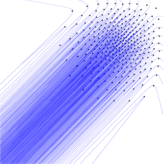
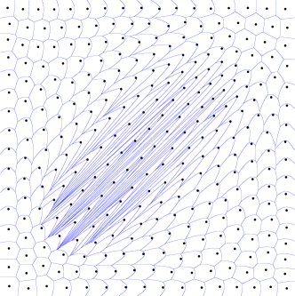
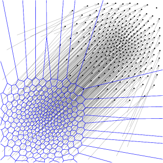
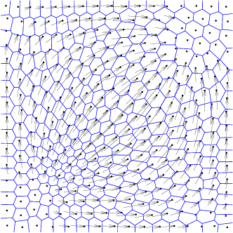
The second column of Figure 5 depicts the measures and and the resulting optimal transport partitions for and . Both partitions look very different from their counterparts when no is added. However the partition for clearly approximates a transport plan along the direction of again. Note that the movement of mass is much more local now, meaning the approximated optimal transport plan is not just obtained by keeping measure in place and moving the remaining measure according to the optimal transport plan approximated in Figure 5(c), but a substantial amount of mass available from is moved as well. Furthermore, Figure 5(d) gives the impression of a slightly curved movement of mass. We attribute this to a combination of a boundary effect from trimming the Lebesgue measure to and numerical error based on the coarse discretization and a small amount of mistransported mass.
The computed -value for this new example (last column of Table 1) lies in the vicinity of the theoretical value again if one allows for the rather large discretization error.
The case exhibits the distinctive curved behavior that goes with the fluid mechanics interpretation discussed in Subsection 1.2, see also Figure 1. Various of the other points mentioned in Subsection 1.2 can be observed as well, e.g. the numerically computed Wasserstein distance is much smaller than for , which illustrates the lack of invariance and seems plausible in view of the example in Remark 2 in the appendix.
6.2 A practical resource allocation problem
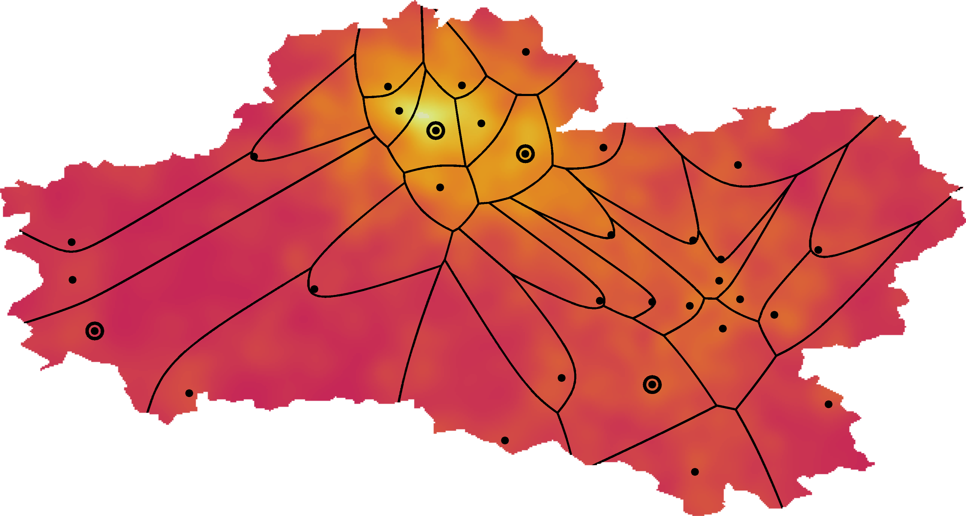
We revisit the delivery problem mentioned in the introduction. A fast-food delivery service has 32 branches throughout a city area, depicted by the black dots on the map in Figure 6. For simplicity of representation we assume that most branches have the same fixed production capacity and a few individual ones (marked by an extra circle around the dot) have twice that capacity. We assume further that the expected orders at peak times have a spatial distribution as indicated by the heatmap (where yellow to white means higher number of orders) and a total volume that matches the total capacity of the branches. The task of the fast-food chain is to partition the map into 32 delivery zones, matching expected orders in each zone with the capacity of the branches, in such a way that the expected cost in form of the travel distance between branch and customer is minimal. We assume here the Euclidean distance, either because of a street layout that comes close to it, see e.g. [9], or because the deliveries are performed by drones. The desired partition, computed by our implementation described in Subsection 4.3, is also displayed in Figure 6. A number of elongated cells in the western and central parts of the city area suggest that future expansions of the fast-food chain should concentrate on the city center in the north.
6.3 A visual tool for detecting deviations from a density map
Very recently, asymptotic theory has been developed that allows, among other things, to test based on the Wasserstein metric whether a sample in comes from a given multivariate probability distribution . More precisely, assuming independent and identically distributed random vectors with distribution , limiting distributions have been derived for suitable standardizations of both if and if . Based on an observed value , where , these distributions allow to assign a level of statistical certainty (p-value) to statements of and , respectively. See [50], which uses general , but requires discrete distributions and ; and [16], which is constraint to , but allows for quite general distributions ( and not both discrete).
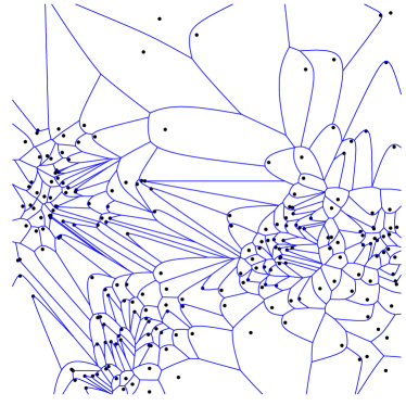
We propose here the optimal transport partition between an absolutely continuous and as a simple but useful tool for assessing the hypothesis . We refer to this tool as goodness-of-fit (GOF) partition. If relevant information may be gained from a simple plot of this partition in a similar way as residual plots are used for assessing the fit of linear models. As a general rule of thumb the partition is consistent with the hypothesis if it consists of many “round” cells that contain their respective -points roughly in their middle. The size of cells may vary according to local densities and there are bound to be some elongated cells due to sampling error (i.e. the fact that we can only sample from and do not know it exactly), but a local accumulation of many elongated cells should give rise to the suspicion that may be violated in a specific way. Thus GOF partitions provide the data scientist both with a global impression for the plausibility of and with detailed local information about the nature of potential deviations of from . Of course they are a purely explorative tool and do not give any quantitative guarantees.
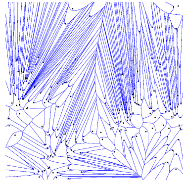
We give here an example for illustration. Suppose we have data as given in the left panel of Figure 7 and a distribution as represented by the heat map in the right panel. Figure 8 shows the optimal transport partition for this situation on the left hand side. The partition indicates that the global fit of the data is quite good. However it also points out some deviations that might be spurious, but might also well be worth further investigation: One is the absence of points close to the two highest peaks in the density map, another one that there are some points too many in the cluster on the very left of the plot. Both of them are quite clearly visible as accumulations of elongated cells.
As an example of a globally bad fit we show in the right panel of Figure 8 the GOF partition when taking as the uniform measure on the square.


For larger direct visual inspection becomes impossible. However, a substantial amount of information may still be extracted, either by considering statistics of the GOF partition in dimensions that are able to detect local regions of common orientation and high eccentricity of cells, or by applying dimension reduction methods, such as [18], before applying the GOF partition.
7 Discussion and outlook
We have given a comprehensive account on semi-discrete optimal transport for the Euclidean cost function, arguing that there are sometimes good reasons to prefer Euclidean over squared Euclidean cost and showing that for the Euclidean case the semi-discrete setting is particularly nice because we obtain a unique solution to the Monge–Kantorovich problem that is induced by a transport map. We have provided a reasonably fast algorithm that is similar to the AHA-algorithm described in detail in [31] but adapted in various aspects to the current situation of .
Our algorithm converges towards the optimal partition subject to the convergence conditions for the L-BFGS algorithm; see e.g. [34]. Very loosely, such conditions state that we start in a region around the minimizer where the objective function shows to some extent quadratic behavior. Similar to the AHA-algorithm in [31], a proof of such conditions is not available. In practice, the algorithm has converged in all the experiments and examples given in the present paper.
There are several avenues for further research, both with regard to improving speed and robustness of the algorithm and for solving more complicated problems where our algorithm may be useful. Some of them are:
-
•
As mentioned earlier, it may well be that the choice of our starting value is too simplistic and that faster convergence is obtained more often if the sequence of coarsenings is e.g. based on the -median algorithm or a similar method. The difficulty lies in finding that makes substantially smaller without investing too much time in its computation.
-
•
We currently keep the threshold in the stopping criterion of the multiscale approach in Subsection 4.1 fixed. Another alleviation of the computational burden may be obtained by choosing a suitable sequence of thresholds for the various scales. It seems particularly attractive to use for the threshold at the coarser scale a value that is smaller than the value at the finer scale, especially for the last step, where . The rationale is that at the coarser scale we do not run easily into numerical problems and still reach the stricter -target efficiently. The obtained weight vector is expected to result in a better starting solution for the finer problem that reaches the more relaxed threshold more quickly than a starting solution stemming from an -target at the coarser scale.
-
•
The L-BFGS algorithm used for the optimization process may be custom-tailored to our discretization of in order to reach the theoretically maximal numerical precision that the discretization allows. It could e.g. use simple gradient descent from the point on where L-BFGS cannot minimize any further since even in the discretized case the gradient always points in a descending direction.
-
•
The approximation of by a fine-grained discrete measure has shown good results. However, as mentioned earlier, higher numerical stability and precision at the expense of complexity and possibly runtime could be obtained by a version of our algorithm that computes the intersections between the Voronoi cells and the pixels of exactly.
-
•
Semi-discrete optimal transport may be used as an auxiliary step in a number of algorithms for more complicated problems. The most natural example is a simple alternating scheme for the capacitated location-allocation (or transportation-location) problem; see [12]. Suppose that our fast-food chain from Subsection 6.2 has not entered the market yet and would like to open branches anywhere in the city and divide up the area into delivery zones in such a way that (previously known) capacity constraints of the branches are met and the expected cost in terms of travel distance is minimized again. A natural heuristic algorithm would start with a random placement of branches and alternate between capacitated allocation of expected orders (the continuous measure ) using our algorithm described in Section 4 and the relocation of branches to the spatial medians of the zones. The latter can be computed by discrete approximation, see e.g. [14], and possibly by continuous techniques, see [17] for a vantage point.
Acknowledgements
The authors thank Marcel Klatt for helpful discussions and an anonymous referee for comments that lead to an improvement of the paper.
References
- Altschuler et al., [2017] Altschuler, J., Weed, J., and Rigollet, P. (2017). Near-linear time approximation algorithms for optimal transport via Sinkhorn iteration. In Proc. NIPS 2017, pages 1961–1971.
- Ambrosio and Pratelli, [2003] Ambrosio, L. and Pratelli, A. (2003). Existence and stability results in the theory of optimal transportation. In Optimal transportation and applications (Martina Franca, 2001), volume 1813 of Lecture Notes in Math., pages 123–160. Springer, Berlin.
- Arjovsky et al., [2017] Arjovsky, M., Chintala, S., and Bottou, L. (2017). Wasserstein generative adversarial networks. In Proceedings of the 34th International Conference on Machine Learning, volume 70 of PMLR, Sydney, Australia.
- Armijo, [1966] Armijo, L. (1966). Minimization of functions having Lipschitz continuous first partial derivatives. Pacific Journal of Mathematics, 16(1).
- Aurenhammer et al., [1998] Aurenhammer, F., Hoffmann, F., and Aronov, B. (1998). Minkowski-type theorems and least-squares clustering. Algorithmica, 20(1):61–76.
- Basua et al., [2014] Basua, S., Kolouria, S., and Rohde, G. K. (2014). Detecting and visualizing cell phenotype differences from microscopy images using transport-based morphometry. PNAS, 111(9):3448—3453.
- Beckmann, [1952] Beckmann, M. (1952). A continuous model of transportation. Econometrica, 20:643–660.
- Benamou and Brenier, [2000] Benamou, J.-D. and Brenier, Y. (2000). A computational fluid mechanics solution to the Monge–Kantorovich mass transfer problem. Numer. Math., 84:375–393.
- Boscoe et al., [2012] Boscoe, F. P., Henry, K. A., and Zdeb, M. S. (2012). A nationwide comparison of driving distance versus straight-line distance to hospitals. Prof. Geogr., 64(2):188–196.
- Bourne et al., [2018] Bourne, D. P., Schmitzer, B., and Wirth, B. (2018). Semi-discrete unbalanced optimal transport and quantization. Preprint. https://arxiv.org/abs/1808.01962v1.
- CGAL2015, [2015] CGAL2015 (2015). CGAL, Computational Geometry Algorithms Library (Version 4.6.1). http://www.cgal.org.
- Cooper, [1972] Cooper, L. (1972). The transportation-location problem. Oper. Res., 20(1):94–108.
- Courty et al., [2016] Courty, N., Flamary, R., Tuia, D., and Corpetti, T. (2016). Optimal transport for data fusion in remote sensing. In 2016 IEEE International Geoscience and Remote Sensing Symposium (IGARSS), pages 3571–3574.
- Croux et al., [2012] Croux, C., Filzmoser, P., and Fritz, H. (2012). A comparison of algorithms for the multivariate -median. Computational Statistics, 27(3):393–410.
- Cuturi, [2013] Cuturi, M. (2013). Sinkhorn distances: Lightspeed computation of optimal transport. In Proc. NIPS 2013, pages 2292–2300.
- del Barrio and Loubes, [2018] del Barrio, E. and Loubes, J.-M. (2018). Central limit theorems for empirical transportation cost in general dimension. Preprint. https://arxiv.org/abs/1705.01299v3.
- Fekete et al., [2005] Fekete, S. P., Mitchell, J. S. B., and Beurer, K. (2005). On the continuous Fermat-Weber problem. Operations Research, 53(1):61–76.
- Flamary et al., [2018] Flamary, R., Cuturi, M., Courty, N., and Rakotomamonjy, A. (2018). Wasserstein discriminant analysis. Machine Learning, 107(12):1923–1945.
- Geiß et al., [2013] Geiß, D., Klein, R., Penninger, R., and Rote, G. (2013). Optimally solving a transportation problem using Voronoi diagrams. Comput. Geom., 46(8):1009–1016.
- Genevay et al., [2016] Genevay, A., Cuturi, M., Peyré, G., and Bach, F. (2016). Stochastic optimization for large-scale optimal transport. In Proc. NIPS 2016, pages 3432–3440.
- Genevay et al., [2018] Genevay, A., Peyré, G., and Cuturi, M. (2018). Learning generative models with Sinkhorn divergences. In Proceedings of the 21st International Conference on Artificial Intelligence and Statistics, volume 84 of PMLR, Lanzarote, Spain.
- Gramfort et al., [2015] Gramfort, A., Peyré, G., and Cuturi, M. (2015). Fast optimal transport averaging of neuroimaging data. In 24th International Conference on Information Processing in Medical Imaging (IPMI 2015), volume 9123 of Lecture Notes in Computer Science, pages 123–160.
- Guo et al., [2017] Guo, J., Pan, Z., Lei, B., and Ding, C. (2017). Automatic color correction for multisource remote sensing images with Wasserstein CNN. Rem. Sens., 9(5):1–16 (electronic).
- Hartmann, [2016] Hartmann, V. (2016). A geometry-based approach for solving the transportation problem with Euclidean cost. Bachelor’s thesis, Institute of Mathematical Stochastics, University of Göttingen. https://arxiv.org/abs/1706.07403.
- Kantorovich, [1942] Kantorovich, L. (1942). On the translocation of masses. C. R. (Doklady) Acad. Sci. URSS (N.S.), 37:199–201.
- Karavelas and Yvinec, [2002] Karavelas, M. I. and Yvinec, M. (2002). Dynamic additively weighted Voronoi diagrams in 2D. In Algorithms – ESA 2002, pages 586–598. Springer.
- Kitagawa et al., [2018] Kitagawa, J., Mérigot, Q., and Thibert, B. (2018). Convergence of a Newton algorithm for semi-discrete optimal transport. J. Eur. Math. Soc., to appear. http://arxiv.org/abs/1603.05579v2.
- Klatt and Munk, [2018] Klatt, M. and Munk, A. (2018). Limit distributions for empirical regularized optimal transport and applications. In preparation.
- Luenberger and Ye, [2008] Luenberger, D. G. and Ye, Y. (2008). Linear and nonlinear programming. International Series in Operations Research & Management Science, 116. Springer, New York, third edition.
- McCann, [1995] McCann, R. J. (1995). Existence and uniqueness of monotone measure-preserving maps. Duke Math. J., 80(2):309–323.
- Mérigot, [2011] Mérigot, Q. (2011). A multiscale approach to optimal transport. Comput. Graph. Forum, 30(5):1583–1592.
- Monge, [1781] Monge, G. (1781). Mémoire sur la théorie des déblais et des remblais. In Histoire de l’Académie Royale des Sciences de Paris, avec les Mémoires de Mathématique et de Physique pour la même année,, pages 666–704.
- Nicolas, [2016] Nicolas, P. (2016). Optimal transport for image processing. Habilitation thesis, Signal and Image Processing, Université de Bordeaux. https://hal.archives-ouvertes.fr/tel-01246096v6.
- Nocedal, [1980] Nocedal, J. (1980). Updating quasi-Newton matrices with limited storage. Mathematics of computation, 35(151):773–782.
- Okazaki and Nocedal, [2010] Okazaki, N. and Nocedal, J. (2010). libLBFGS (Version 1.10). http://www.chokkan.org/software/liblbfgs/.
- Peyré and Cuturi, [2018] Peyré, G. and Cuturi, M. (2018). Computational Optimal Transport. now Publishers. https://arxiv.org/abs/1803.00567.
- Pratelli, [2007] Pratelli, A. (2007). On the equality between Monge’s infimum and Kantorovich’s minimum in optimal mass transportation. Ann. Inst. H. Poincaré Probab. Statist., 43(1):1–13.
- R Core Team, [2017] R Core Team (2017). R: A Language and Environment for Statistical Computing. R Foundation for Statistical Computing, Vienna, Austria. Version 3.3.0. https://www.R-project.org/.
- Rippl et al., [2016] Rippl, T., Munk, A., and Sturm, A. (2016). Limit laws of the empirical Wasserstein distance: Gaussian distributions. J. Multivar. Anal., 151:90–109.
- Santambrogio, [2015] Santambrogio, F. (2015). Optimal transport for applied mathematicians, volume 87 of Progress in Nonlinear Differential Equations and their Applications. Birkhäuser/Springer, Cham.
- Schmitz et al., [2018] Schmitz, M. A., Heitz, M., Bonneel, N., Ngolè, F., Coeurjolly, D., Cuturi, M., Peyré, G., and Starck, J.-L. (2018). Wasserstein dictionary learning: Optimal transport-based unsupervised nonlinear dictionary learning. SIAM Journal on Imaging Sciences, 11(1):643–678.
- [42] Schmitzer, B. (2016a). A sparse multiscale algorithm for dense optimal transport. J Math Imaging Vis, 56(2):238–259.
- [43] Schmitzer, B. (2016b). Stabilized sparse scaling algorithms for entropy regularized transport problems. Preprint. https://arxiv.org/abs/1610.06519v1.
- Schmitzer and Wirth, [2018] Schmitzer, B. and Wirth, B. (2018). A framework for Wasserstein-1-type metrics. Preprint. http://arxiv.org/abs/1701.01945v2.
- Schrieber et al., [2017] Schrieber, J., Schuhmacher, D., and Gottschlich, C. (2017). DOTmark — a benchmark for discrete optimal transport. IEEE Access, 5.
- Schuhmacher et al., [2018] Schuhmacher, D., Bähre, B., Gottschlich, C., Heinemann, F., and Schmitzer, B. (2018). transport: Optimal Transport in Various Forms. R package version 0.9-4. https://cran.r-project.org/package=transport.
- Sherali and Nordai, [1988] Sherali, H. D. and Nordai, F. L. (1988). NP-hard, capacitated, balanced p-median problems on a chain graph with a continuum of link demands. Math. Oper. Res., 13(1):32–49.
- Solomon et al., [2015] Solomon, J., de Goes, F., Peyré, G., Cuturi, M., Butscher, A., Nguyen, A., Du, T., and Guibas, L. (2015). Convolutional Wasserstein distances: Efficient optimal transportation on geometric domains. ACM Trans. Graph., 34(4):66:1–66:11.
- Solomon et al., [2014] Solomon, J., Rustamov, R., Guibas, L., and Butscher, A. (2014). Convolutional Wasserstein distances: Efficient optimal transportation on geometric domains. ACM Trans. Graph., 33(4):67:1–67:12.
- Sommerfeld and Munk, [2018] Sommerfeld, M. and Munk, A. (2018). Inference for empirical Wasserstein distances on finite spaces. Journal of the Royal Statistical Society: Series B (Statistical Methodology), 80(1):219–238.
- Villani, [2009] Villani, C. (2009). Optimal transport, old and new, volume 338 of Grundlehren der Mathematischen Wissenschaften [Fundamental Principles of Mathematical Sciences]. Springer-Verlag, Berlin.
- Wolansky, [2015] Wolansky, G. (2015). Semi-discrete approximation of optimal mass transport. Preprint. http://arxiv.org/abs/1502.04309v1.
- Wolfe, [1969] Wolfe, P. (1969). Convergence conditions for ascent methods. SIAM Rev., 11:226–235.
- Wolfe, [1971] Wolfe, P. (1971). Convergence conditions for ascent methods. II. Some corrections. SIAM Rev., 13:185–188.
Valentin Hartmann
IC IINFCOM DLAB
EPFL
Station 14
1015 Lausanne, Switzerland
E-mail: valentin.hartmann@epfl.ch
Dominic Schuhmacher
Institute for Mathematical Stochastics
University of Goettingen
Goldschmidtstr. 7
37077 Göttingen, Germany
E-mail: schuhmacher@math.uni-goettingen.de
Appendix: Formulae for affine transformations of measures
We have the following relations when adding a common measure or multiplying by a common nonnegative scalar. The proof easily extends to a complete separable metric space instead of equipped with the Euclidean metric.
Lemma 1.
Let be finite measures on satisfying . For and , we have
| (12) | ||||
| (13) | ||||
| (14) |
where we assume for that .
Proof.
Write . Denote by the push-forward of under the map . Let be an optimal transport plan for the computation of . Then is a feasible transport plan for that generates the same total cost as . Thus
Likewise is a feasible transport plan for that generates times the cost of for the integral in (1). Thus
Replacing by , as well as by and by , we obtain (14).
It remains to show . For this we use that a transport plan between and is optimal if and only if it is cyclical monotone, meaning that for all and all , we have
where ; see [51, Theorem 5.10(ii) and Definition 5.1].
Letting be an optimal transport plan for the computation of , we show optimality of for the computation of . We know that is cyclical monotone. Let and . Denote by , where , the indices of all pairs with , and hence . By the cyclical monotonicity of (writing ) and the triangle inequality, we obtain
Thus is cyclical monotone and since it is a feasible transport plan between and , it is optimal for the computation of , which concludes the proof. ∎
Remark 2.
Equation (13) is not generally true for any . To see this consider the case , , and , where . Clearly for all . Denote by and the cumulative distribution functions (CDFs) of and , respectively, i.e. and for all . Thus
We then even obtain
as if . For the first equality we used the representation of in terms of (generalized) inverses of their CDFs; see Equation (2) in [39] and the references given there and note that the generalization from the result for probability measures is immediate by (14).