Privacy Preserving Randomized Gossip Algorithms

Filip Hanzely    Jakub Konečný    Nicolas Loizou    Peter Richtárik⋄⋆    Dmitry Grishchenko
xxx
University of Edinburgh, UK
KAUST, KSA
Higher School of Economics, Russia
(June 21, 2017)
Abstract

In this work we present three different randomized gossip algorithms for solving the average consensus problem while at the same time protecting the information about the initial private values stored at the nodes. We give iteration complexity bounds for all methods, and perform extensive numerical experiments.

1 Introduction

In this paper we consider the average consensus (AC) problem. Let 𝒢=(𝒱,)𝒢𝒱{\cal G}=({\cal V},{\cal E}) be an undirected connected network with node set 𝒱={1,2,,n}𝒱12𝑛{\cal V}=\{1,2,\dots,n\} and edges {\cal E} such that ||=m𝑚|{\cal E}|=m. Each node i𝒱𝑖𝒱i\in{\cal V} “knows” a private value cisubscript𝑐𝑖c_{i}\in\mathbb{R}. The goal of AC is for every node of the network to compute the average of these values, c¯=def1nici¯𝑐def1𝑛subscript𝑖subscript𝑐𝑖\bar{c}\overset{\text{def}}{=}\tfrac{1}{n}\sum_{i}c_{i}, in a distributed fashion. That is, the exchange of information can only occur between connected nodes (neighbours).

The literature on methods for solving the average consensus problem is vast and has long history [52, 51, 4, 30]. The algorithms for solving this problem can be divided in two broad categories: the average consensus algorithms [54] and the gossip algorithms [5, 49]. The main difference is that the former work in a synchronous setting while the gossip algorithms model the case of asynchronous setting. In the average consensus algorithms, all nodes of the network update their values simultaneously by communicate with a set of their neighbours and in all iterations the same update occurs. In gossip algorithms, at each iteration, only one edge is selected randomly, and the corresponding nodes update their values to their average. In this work we focus on randomized gossip algorithms and propose techniques for protecting information of the initial values cisubscript𝑐𝑖c_{i}, in the case when these may be sensitive.

In this work we develop and analyze three private variants of the randomized pairwise gossip algorithm for solving the average consensus problem. As an additional requirement we wish to prevent nodes to “learn” information about the private values of other nodes. While we shall not formalize the notion of privacy preservation in this work, it will be intuitively clear that our methods indeed make it harder for nodes to infer information about the private values of other nodes.

1.1 Background

The average consensus problem and randomized gossip algorithms for solving it appear in many applications, including distributed data fusion in sensor networks [55], load balancing [10] and clock synchronization [18]. This subject was first introduced in [52], and was studied extensively in the last decade; the seminal 2006 paper of Boyd et al. [5] on randomized gossip algorithms motivated a large amount of subsequent research and generated more than 150015001500 citations to date.

In this work, we focus on modifying the basic algorithm of [5], which we refer to as “Standard Gossip” algorithm. In the following, we review several avenues of research the gossip algorithms were evolved. While we do not address any privacy considerations in these settings, they can serve as inspiration for further work. For a survey of relevant work prior to 2010, we refer the reader to reviews in [12, 40, 45].

The Geographic Gossip algorithm was proposed in [11], in which the authors combine the gossip approach with a geographic routing towards a randomly chosen location with main goal the improvement of the convergence rate of Standard Gossip algorithm. In each step, a node is activated, assuming that it is aware of its geographic location and some additional assumptions on the network topology, it chooses another node from the rest of the network (not necessarily one of its neighbours) and performs a pairwise averaging with this node. Later, using the same assumptions, this algorithm was extended into Geographic Gossip Algorithm with Path Averaging [3], in which connected sequences of nodes were chosen in each step and they averaged their values. More recently, in [19] and [20] authors propose a geographic and path averaging methods which converge to the average consensus without the assumption that nodes are aware of their geographic location.

Another important class of randomized gossip algorithms are the Broadcast Gossip algorithms, firts proposed in [2] and then extended in [17, 53, 29]. The idea of this algorithm is simple: In each step a node in the network is activated uniformly at random, following the asynchronous time model, and broadcasts its value to its neighbours. The neighbours receive this value and update their own values. It was experimentally shown that this method converge faster than the pairwise and geographic randomized gossip algorithms.

Alternative approach to the gossip framework are so called non-randomized Gossip algorithms [38, 27, 34, 56]. Typically, this class of algorithms executes the pairwise exchanges between nodes in a deterministic, such as pre-defined cyclic, order. T𝑇T-periodic gossiping is a protocol which stipulates that each node must interact with each of its neighbours exactly once every T𝑇T time units. Under suitable connectivity assumptions of the network 𝒢𝒢\mathcal{G}, the T𝑇T-periodic gossip sequence will converge at a rate determined by the magnitude of the second largest eigenvalue of the stochastic matrix determined by the sequence of pairwise exchanges which occurs over a period. It has been shown that if the underlying graph is a tree, this eigenvalue is the same for all possible T𝑇T-periodic gossip protocols.

A different approach, uses memory in the update of the values each node holds, to get Accelerated Gossip algorithms. The nodes update their value using an update rule that involve not only the current values of the sampled nodes but also their previous values. This idea is closely related to the shift register methods studied in numerical linear algebra for improving the convergence rate of linear system solvers. The works [6, 33] have shown theoretically and numerically, that under specific assumptions this idea can improve the performance of the Standard Gossip algorithm.

Randomized Kaczmarz-type Gossip algorithms. Very recently has been proved that popular randomized Kaczmarz-type methods for solving large linear systems can also solve the AC problem. In particular, in [23] and [35] it was shown how that existing Randomized Kaczmarz and Randomized Block Kaczmarz methods can be interpreted as randomized gossip algorithms for solving the AC problem, by solving a particular system encoding the underlying network structure. This approach was the first time that a connection between the two research areas of linear system solvers and distributed algorithms have been established.

In this work we are interested in the asynchronous time model [5, 4]. More precisely, we assume that each node of our network has a clock which ticks at a rate of 111 Poisson process. This is equivalent of having available a global clock which ticks according to a rate n𝑛n Poisson process and selects an edge of the network uniformly at random. In general the synchronous setting (all nodes update the values of their nodes simultaneously using information from a set of their neighbours) is convenient for theoretical considerations, but is not representative of some practical scenarios, such as the distributed nature of sensor networks. For more details on clock modelling we refer the reader to [5], as the contribution of this paper is orthogonal to these considerations.

Privacy and Average Consensus. Finally, the introduction of notions of privacy within the AC problem is relatively recent in the literature, and the existing works consider two different ideas.

The concept of differential privacy [13] is used to protect the output value c¯¯𝑐\bar{c} computed by all nodes in [28]. In this work, an exponentially decaying Laplacian noise is added to the consensus computation. This notion of privacy refers to protection of the final average, and formal guarantees are provided.

A different goal is the protection of the initial values cisubscript𝑐𝑖c_{i} the nodes know at the start. In [36, 37], the goal is to make sure that each node is unable to infer a lot about the initial values cisubscript𝑐𝑖c_{i} of any other node. Both of these methods add noise correlated across individual iterations, to make sure they converge to the exact average. A formal notion of privacy breach is formulated in [37], in which they also show that their algorithm is optimal in that particular sense.

1.2 Main Contributions

In this work we present three different approaches for solving the Average Consensus problem while at the same time protecting the information about the initial values. All of the above mentioned works focus on the synchronous setting of the AC problem. This work is the first which combines the gossip framework with the privacy concept of protection of the initial values. It is important to stress that we provide tools for protection of the initial values, but we do not address any specific notion of privacy or a threat model, nor how these quantitatively translate to any explicit measure. These would be highly application dependent, and we only provide theoretical convergence rates for the techniques we propose.

The methods we propose are all dual in nature. The dual approach is explained in detail in Section 2. It was first proposed for solving linear systems in [23] and then extend to the concept of average consensus problems in [35]. The dual updates immediately correspond to updates to the primal variables, via an affine mapping. One of the contributions of our work is that we exactly recover existing convergence rates for the primal iterates as a special case.

We now outline the three different techniques we propose in this paper, which we refer to as “Binary Oracle”, “ϵitalic-ϵ\epsilon-Gap Oracle” and “Controlled Noise Insertion”. The first two are, to the best of our knowledge, the first proposal of weakening the oracle used in the gossip framework. The latter is inspired by and similar to the addition of noise proposed in [37] for the synchronous setting. We extend this technique by providing explicit finite time convergence guarantees.

Binary Oracle. The difference from standard Gossip algorithms we propose is to reduce the amount of information transmitted in each iteration to a single bit. More precisely, when an edge is selected, each corresponding node will only receive information whether the value on the other node is smaller or larger. Instead of setting the value on each node to their average, each node increases or decreases its value by a pre-specified step.

ϵitalic-ϵ\epsilon-Gap Oracle. In this case, we have an oracle that returns one of three options, and is parametrized by ϵitalic-ϵ\epsilon. If the difference in values of sampled nodes is larger than ϵitalic-ϵ\epsilon, an update similar to the one in Binary Oracle is taken. Otherwise, the values remain unchanged. An advantage compared to the Binary Oracle is that this approach will converge to a certain accuracy and stop there, determined by ϵitalic-ϵ\epsilon (Binary Oracle will oscillate around optimum for a fixed stepsize). However, in general it will disclose more information about the initial values.

Controlled Noise Insertion. This approach is inspired by the works of [36, 37], and protects the initial values by inserting noise in the process. Broadly speaking, in each iteration, each of the sampled nodes first add a noise to its current value, and an average is computed afterwards. Convergence is guaranteed because of correlation in the noise across iterations. Each node remembers the noise it added last time it was sampled, and in the following iteration, the previously added noise is first subtracted, and a fresh noise of smaller magnitude is added.

Empirically, the protection of initial values is provided by first injecting noise in the system, which propagates across network, but is gradually withdrawn to ensure convergence to the true average.

Main Results
Randomized Gossip Methods Convergence Rate Success Measure Thm
Standard Gossip [5] (1α(𝒢)2m)ksuperscript1𝛼𝒢2𝑚𝑘\left(1-\frac{\alpha({\cal G})}{2m}\right)^{k} 𝔼[12c¯𝟏xk2]𝔼delimited-[]12superscriptnorm¯𝑐1superscript𝑥𝑘2{\mathbb{E}\left[\tfrac{1}{2}\|\bar{c}{\bf 1}-x^{k}\|^{2}\right]} 5
New: Private Gossip with Binary Oracle 1/k1𝑘1/\sqrt{k} mintk𝔼[1me|xitxjt|]subscript𝑡𝑘𝔼delimited-[]1𝑚subscript𝑒subscriptsuperscript𝑥𝑡𝑖subscriptsuperscript𝑥𝑡𝑗\min_{t\leq k}{\mathbb{E}\left[\frac{1}{m}\sum_{e}|x^{t}_{i}-x^{t}_{j}|\right]} 6
New: Private Gossip with ϵitalic-ϵ\epsilon-Gap Oracle 1/(kϵ2)1𝑘superscriptitalic-ϵ21/(k\epsilon^{2}) 𝔼[1kt=0k1Δt(ϵ)]𝔼delimited-[]1𝑘superscriptsubscript𝑡0𝑘1superscriptΔ𝑡italic-ϵ{\mathbb{E}\left[\frac{1}{k}\sum_{t=0}^{k-1}\Delta^{t}(\epsilon)\right]} 9
New: Private Gossip with Controlled Noise Insertion (1min(α(𝒢)2m,γm))ksuperscript1𝛼𝒢2𝑚𝛾𝑚𝑘\left(1-\min\left(\frac{\alpha({\cal G})}{2m},\frac{\gamma}{m}\right)\right)^{k} 𝔼[D(y)D(yk)]𝔼delimited-[]𝐷superscript𝑦𝐷superscript𝑦𝑘{\mathbb{E}\left[D(y^{*})-D(y^{k})\right]} 11
Table 1: Complexity results of all proposed gossip algorithms.

Convergence Rates of our Methods. In Table 1, we present summary of convergence guarantees for the above three techniques. By \|\cdot\| we denote the standard Euclidean norm.

The two approaches to restricting the amount of information disclosed, Binary Oracle and ϵitalic-ϵ\epsilon-Gap Oracle, converge slower than the standard Gossip. In particular, these algorithms have sublinear convergence rate. At first sight, this should not be surprising, since we indeed use much less information. However, in Theorem 7, we show that if we had in a certain sense perfect global information, we could use it to construct a sequence of adaptive stepsizes, which would push the capability of the binary oracle to a linear convergence rate. However, this rate is still m𝑚m-times slower than the standard rate of the binary gossip algorithm. We note, however, that having global information at hand is an impractical assumption. Nevertheless, this result highlights that there is a potentially large scope for improvement, which we leave for future work.

These two oracles could be in practice implemented using established secure multiparty computation protocols [8]. However, this would require the sampled nodes to exchange more than a single message in each iteration. This is inferior to the requirements of the standard gossip algorithm, but the concern of communication efficiency is orthogonal to the contribution of this work, and we do not address it further.

The approach of Controlled Noise Insertion yields a linear convergence rate which is driven by maximum of two factors. Without going into details, which of these is bigger depends on the speed by which the magnitude of the inserted noise decays. If the noise decays fast enough, we recover the convergence rate of standard the gossip algorithm. In the case of slow decay, the convergence is driven by this decay. By α(𝒢)𝛼𝒢\alpha({\cal G}) we denote the algebraic connectivity of graph 𝒢𝒢{\cal G} [16]. The parameter γ𝛾\gamma controls the decay speed of the inserted noise, see (20).

1.3 Measures of Success

Second major distinction to highlight is that convergence of each of these proposals naturally depend on a different measure of suboptimality. All of them go to 00 as we approach optimal solution. The details of these measures will be described later in the main body, but we give a brief summary of their connections below.

The standard Gossip and Controlled Noise Insertion depend on the same quantity, but we present the latter in terms of dual values as this is what our proofs are based on. Lemma 1 formally specifies this equivalence. The binary oracle depends on average difference among directly connected nodes. The measure for the ϵitalic-ϵ\epsilon-Gap Oracle depends on quantities Δt(ϵ)=1m|{(i,j):|xitxjt|ϵ}|superscriptΔ𝑡italic-ϵ1𝑚conditional-set𝑖𝑗superscriptsubscript𝑥𝑖𝑡superscriptsubscript𝑥𝑗𝑡italic-ϵ\Delta^{t}(\epsilon)=\frac{1}{m}\left|\{(i,j)\in{\cal E}:|x_{i}^{t}-x_{j}^{t}|\geq\epsilon\}\right|, which is the number of edges, connecting nodes, values of which differ by more than ϵitalic-ϵ\epsilon.

To draw connection between these measures, we provide the following lemma, proved in the Appendix. The dual function D𝐷D is formally defined in Section 2.

Lemma 1.

(Relationship between convergence measures) Suppose that x𝑥x is primal variable corresponding to the dual variable y𝑦y as defined in (9). Dual suboptimality can be expressed as the following [23]:

D(y)D(y)=12c¯𝟏x2.𝐷superscript𝑦𝐷𝑦12superscriptnorm¯𝑐1𝑥2D(y^{*})-D(y)=\tfrac{1}{2}\|\bar{c}{\bf 1}-x\|^{2}. (1)

Moreover, for any xn𝑥superscript𝑛x\in\mathbb{R}^{n} we have :

12ni=1nj=1n(xjxi)212𝑛superscriptsubscript𝑖1𝑛superscriptsubscript𝑗1𝑛superscriptsubscript𝑥𝑗subscript𝑥𝑖2\displaystyle\frac{1}{2n}\sum_{i=1}^{n}\sum_{j=1}^{n}(x_{j}-x_{i})^{2} =\displaystyle= c¯𝟏x2superscriptnorm¯𝑐1𝑥2\displaystyle\|\bar{c}{\bf 1}-x\|^{2} (2)
e=(i,j)|xixj|subscript𝑒𝑖𝑗subscript𝑥𝑖subscript𝑥𝑗\displaystyle\sum_{e=(i,j)\in{\cal E}}|x_{i}-x_{j}| \displaystyle\leq mnc¯𝟏x,𝑚𝑛norm¯𝑐1𝑥\displaystyle\sqrt{mn}\|\bar{c}{\bf 1}-x\|, (3)
e=(i,j)|xixj|subscript𝑒𝑖𝑗subscript𝑥𝑖subscript𝑥𝑗\displaystyle\sum_{e=(i,j)\in{\cal E}}|x_{i}-x_{j}| \displaystyle\geq α(𝒢)c¯𝟏x,𝛼𝒢norm¯𝑐1𝑥\displaystyle\sqrt{\alpha({\cal G})}\|\bar{c}{\bf 1}-x\|, (4)
e=(i,j)|xixj|subscript𝑒𝑖𝑗subscript𝑥𝑖subscript𝑥𝑗\displaystyle\sum_{e=(i,j)\in{\cal E}}|x_{i}-x_{j}| \displaystyle\geq ϵ|{(i,j):|xixj|ϵ}|.italic-ϵconditional-set𝑖𝑗subscript𝑥𝑖subscript𝑥𝑗italic-ϵ\displaystyle\epsilon\left|\{(i,j)\in{\cal E}:|x_{i}-x_{j}|\geq\epsilon\}\right|. (5)

1.4 Outline

The remainder of this paper is organized as follows: Section 2 introduces the basic setup that are used through the paper. A detailed explanation of the duality behind the randomized pairwise gossip algorithm is given. We also include a novel and insightful dual analysis of this method as it will make it easier to the reader to parse later development. In Section 3 we present our three private gossip algorithms as well as the associated iteration complexity results. Section 4 is devoted to the numerical evaluation of our methods. Finally, conclusions are drawn in Section 5. All proofs not included in the main text can be found in the Appendix.

2 Dual Analysis of Randomized Pairwise Gossip

As we outlined in the introduction, our approach to extending the (standard) randomized pairwise gossip algorithm to privacy preserving variants utilizes duality. The purpose of this section is to formalize this duality, following the development in [23]. In addition, we provide a novel and self-contain dual analysis of randomized pairwise gossip. While this is of an independent interest, we include the proofs as their understanding aids in the understanding of the more involved proofs of our private gossip algorithms developed in the remainder of the paper.

2.1 Primal and Dual Problems

Consider solving the (primal) problem of projecting a given vector c=x0n𝑐superscript𝑥0superscript𝑛c=x^{0}\in\mathbb{R}^{n} onto the solution space of a linear system:

minxn{P(x)=def12xx02}subject to𝐀x=b,subscript𝑥superscript𝑛𝑃𝑥def12superscriptnorm𝑥superscript𝑥02subject to𝐀𝑥𝑏\min_{x\in\mathbb{R}^{n}}\{P(x)\overset{\text{def}}{=}\tfrac{1}{2}\|x-x^{0}\|^{2}\}\quad\text{subject to}\quad{\bf A}x=b, (6)

where 𝐀m×n𝐀superscript𝑚𝑛{\bf A}\in\mathbb{R}^{m\times n}, bm𝑏superscript𝑚b\in\mathbb{R}^{m}, x0nsuperscript𝑥0superscript𝑛x^{0}\in\mathbb{R}^{n}. We assume the problem is feasible, i.e., that the system 𝐀x=b𝐀𝑥𝑏{\bf A}x=b is consistent. With the above optimization problem we associate the dual problem

maxymD(y)=def(b𝐀x0)y12𝐀y2.subscript𝑦superscript𝑚𝐷𝑦defsuperscript𝑏𝐀superscript𝑥0top𝑦12superscriptnormsuperscript𝐀top𝑦2\max_{y\in\mathbb{R}^{m}}D(y)\overset{\text{def}}{=}(b-{\bf A}x^{0})^{\top}y-\tfrac{1}{2}\|{\bf A}^{\top}y\|^{2}. (7)

The dual is an unconstrained concave (but not necessarily strongly concave) quadratic maximization problem. It can be seen that as soon as the system 𝐀x=b𝐀𝑥𝑏{\bf A}x=b is feasible, the dual problem is bounded. Moreover, all bounded concave quadratics in msuperscript𝑚\mathbb{R}^{m} can be written in the as D(y)𝐷𝑦D(y) for some matrix 𝐀𝐀{\bf A} and vectors b𝑏b and x0superscript𝑥0x^{0} (up to an additive constant).

With any dual vector y𝑦y we associate the primal vector via an affine transformation:

x(y)=x0+𝐀y.𝑥𝑦superscript𝑥0superscript𝐀top𝑦x(y)=x^{0}+{\bf A}^{\top}y.

It can be shown that if ysuperscript𝑦y^{*} is dual optimal, then x=x(y)superscript𝑥𝑥superscript𝑦x^{*}=x(y^{*}) is primal optimal. Hence, any dual algorithm producing a sequence of dual variables ytysuperscript𝑦𝑡superscript𝑦y^{t}\to y^{*} gives rise to a corresponding primal algorithm producing the sequence xt=defx(yt)xsuperscript𝑥𝑡def𝑥superscript𝑦𝑡superscript𝑥x^{t}\overset{\text{def}}{=}x(y^{t})\to x^{*}. We shall now consider one such dual algorithm.

2.2 Stochastic Dual Subspace Ascent

SDSA [23] is a stochastic method for solving the dual problem (7). If we assume that b=0𝑏0b=0, the iterates of SDSA take the form

yt+1=yt𝐒t(𝐒t𝐀𝐀𝐒t)𝐒t𝐀(x0+𝐀yt),superscript𝑦𝑡1superscript𝑦𝑡subscript𝐒𝑡superscriptsuperscriptsubscript𝐒𝑡topsuperscript𝐀𝐀topsubscript𝐒𝑡superscriptsubscript𝐒𝑡top𝐀superscript𝑥0superscript𝐀topsuperscript𝑦𝑡y^{t+1}=y^{t}-{\bf S}_{t}({\bf S}_{t}^{\top}{\bf A}{\bf A}^{\top}{\bf S}_{t})^{\dagger}{\bf S}_{t}^{\top}{\bf A}(x^{0}+{\bf A}^{\top}y^{t}), (8)

where 𝐒tsubscript𝐒𝑡{\bf S}_{t} is a random matrix drawn from independently at each iteration t𝑡t from an arbitrary but fixed distribution 𝒟𝒟{\cal D}, and \dagger denotes the Moore-Penrose pseudoinverse.

The corresponding primal iterates are defined via:

xt=defx(yt)=x0+𝐀ytsuperscript𝑥𝑡def𝑥superscript𝑦𝑡superscript𝑥0superscript𝐀topsuperscript𝑦𝑡x^{t}\overset{\text{def}}{=}x(y^{t})=x^{0}+{\bf A}^{\top}y^{t} (9)

The relevance of this all to average consensus follows through the observation, as we shall see next, that for a specific choice of matrix 𝐀𝐀{\bf A} (as defined in the next subsection) and distribution 𝒟𝒟{\cal D}, method (9) is equivalent to the (standard) randomized pairwise gossip method. In that case, SDSA is a dual variant of randomized pairwise gossip. In particular, we define 𝒟𝒟{\cal D} as follows: Stsubscript𝑆𝑡S_{t} is a unit basis vector in msuperscript𝑚\mathbb{R}^{m}, chosen uniformly at random from the collection of all such unit basis vectors, denoted {fe|e}conditional-setsubscript𝑓𝑒𝑒\{f_{e}\;|\;e\in{\cal E}\}. In this case, SDSA is a randomized coordinate ascent method applied to the dual problem.

For general distributions 𝒟𝒟{\cal D}, the primal methods obtained from SDSA via (9) (but without observing that it arises that way) was fist proposed and studied in [22] under a full rank assumption on 𝐀𝐀{\bf A}. This assumption was lifted, and duality exposed and studied as we explain it here, in [23]. For deeper insights and connections to stochastic optimization, stochastic fixed point methods, stochastic linear systems and probabilistic intersection problems, we refer the reader to [48]. The method can be extended to compute the inverse [25] and pseudoinverse [24] of a matrix, in which case it has deep connections with quasi-Newton updates [25]. In particular, it can be used to design a stochastic block extension of the famous BFGS method [25] and applied to the empirical risk minimization problem arising in machine learning to design a fast stochastic quasi-Newton training method [21].

2.3 Randomized Gossip Setup: Choosing 𝐀𝐀{\bf A}

We wish (𝐀,b)𝐀𝑏({\bf A},b) to be an average consensus (AC) system, defined next.

Definition 2.

([35]) Let 𝒢=(𝒱,)𝒢𝒱{\cal G}=({\cal V},{\cal E}) be an undirected graph with |𝒱|=n𝒱𝑛|{\cal V}|=n and ||=m𝑚|{\cal E}|=m. Let 𝐀𝐀{\bf A} be a real matrix with n𝑛n columns. The linear system 𝐀x=b𝐀𝑥𝑏{\bf A}x=b is an “average consensus (AC) system” for graph 𝒢𝒢{\cal G} if 𝐀x=b𝐀𝑥𝑏{\bf A}x=b iff xi=xjsubscript𝑥𝑖subscript𝑥𝑗x_{i}=x_{j} for all (i,j)𝑖𝑗(i,j)\in{\cal E}.

Note that if 𝐀x=b𝐀𝑥𝑏{\bf A}x=b is an AC system, then the solution of the primal problem (6) is necessarily x=c¯𝟏superscript𝑥¯𝑐1x^{*}=\bar{c}\cdot{\bf 1}, where c¯=1ni=1nxi0.¯𝑐1𝑛superscriptsubscript𝑖1𝑛subscriptsuperscript𝑥0𝑖\bar{c}=\frac{1}{n}\sum_{i=1}^{n}x^{0}_{i}. This is exactly what we want: we want the solution of the primal problem to be xi=c¯subscriptsuperscript𝑥𝑖¯𝑐x^{*}_{i}=\bar{c} for all i𝑖i: the average of the private values stored at the nodes.

It is easy to see that a linear system is an AC system precisely when b=0𝑏0b=0 and the nullspace of 𝐀𝐀{\bf A} is {t𝟏:t}conditional-set𝑡1𝑡\{t{\bf 1}:t\in\mathbb{R}\}, where 𝟏1{\bf 1} is the vector of all ones in nsuperscript𝑛\mathbb{R}^{n}. Hence, 𝐀𝐀{\bf A} has rank n1𝑛1n-1.

In the rest of this paper we focus on a specific AC system; one in which the matrix 𝐀𝐀{\bf A} is the incidence matrix of the graph 𝒢𝒢{\cal G} (see Model 1 in [23]). In particular, we let 𝐀m×n𝐀superscript𝑚𝑛{\bf A}\in\mathbb{R}^{m\times n} be the matrix defined as follows. Row e=(i,j)𝑒𝑖𝑗e=(i,j)\in{\cal E} of 𝐀𝐀{\bf A} is given by 𝐀ei=1subscript𝐀𝑒𝑖1{\bf A}_{ei}=1, 𝐀ej=1subscript𝐀𝑒𝑗1{\bf A}_{ej}=-1 and 𝐀el=0subscript𝐀𝑒𝑙0{\bf A}_{el}=0 if l{i,j}𝑙𝑖𝑗l\notin\{i,j\}. Notice that the system 𝐀x=0𝐀𝑥0{\bf A}x=0 encodes the constraints xi=xjsubscript𝑥𝑖subscript𝑥𝑗x_{i}=x_{j} for all (i,j)𝑖𝑗(i,j)\in{\cal E}, as desired.

2.4 Randomized Pairwise Gossip

We provide both primal and dual form of the (standard) randomized pairwise gossip algorithm.

The primal form is standard and needs no lengthy commentary. At the beginning of the process, node i𝑖i contains private information ci=xi0subscript𝑐𝑖subscriptsuperscript𝑥0𝑖c_{i}=x^{0}_{i}. In each iteration we sample a pair of connected nodes (i,j)𝑖𝑗(i,j)\in{\cal E} uniformly at random, and update xisubscript𝑥𝑖x_{i} and xjsubscript𝑥𝑗x_{j} to their average. We let the values at the remaining nodes intact.

Input: vector of private values cn𝑐superscript𝑛c\in\mathbb{R}^{n}
Initialize: Set x0=csuperscript𝑥0𝑐x^{0}=c.
for t=0,1,,k1𝑡01𝑘1t=0,1,\dots,k-1 do
      
  1. 1.

    Choose node e=(i,j)𝑒𝑖𝑗e=(i,j)\in{\cal E} uniformly at random

  2. 2.

    Update the primal variable:

    xlt+1={xit+xjt2,l{i,j}xlt,l{i,j}.subscriptsuperscript𝑥𝑡1𝑙casessubscriptsuperscript𝑥𝑡𝑖subscriptsuperscript𝑥𝑡𝑗2𝑙𝑖𝑗subscriptsuperscript𝑥𝑡𝑙𝑙𝑖𝑗x^{t+1}_{l}=\begin{cases}\frac{x^{t}_{i}+x^{t}_{j}}{2},\quad&l\in\{i,j\}\\ x^{t}_{l},\quad&l\notin\{i,j\}.\end{cases}
end for
return xksuperscript𝑥𝑘x^{k}
Algorithm 1 (Primal form)

The dual form of the standard randomized pairwise gossip method is a specific instance of SDSA, as described in (8), with x0=csuperscript𝑥0𝑐x^{0}=c and 𝐒tsubscript𝐒𝑡{\bf S}_{t} being a randomly chosen standard unit basis vector fesubscript𝑓𝑒f_{e} in msuperscript𝑚\mathbb{R}^{m} (e𝑒e is a randomly selected edge). It can be seen [23] that in that case, (8) takes the following form:

Input: vector of private values cn𝑐superscript𝑛c\in\mathbb{R}^{n}
Initialize: Set y0=0msuperscript𝑦00superscript𝑚y^{0}=0\in\mathbb{R}^{m}.
for t=0,1,,k1𝑡01𝑘1t=0,1,\dots,k-1 do
      
  1. 1.

    Choose node e=(i,j)𝑒𝑖𝑗e=(i,j)\in{\cal E} uniformly at random

  2. 2.

    Update the dual variable:

    yt+1=yt+λtfewhereλt=argmaxλD(yt+λfe).formulae-sequencesuperscript𝑦𝑡1superscript𝑦𝑡superscript𝜆𝑡subscript𝑓𝑒wheresuperscript𝜆𝑡subscriptargmaxsuperscript𝜆𝐷superscript𝑦𝑡superscript𝜆subscript𝑓𝑒y^{t+1}=y^{t}+\lambda^{t}f_{e}\quad\mathrm{where}\quad\lambda^{t}=\mathrm{argmax}_{\lambda^{\prime}}D(y^{t}+\lambda^{\prime}f_{e}).
end for
return yksuperscript𝑦𝑘y^{k}
Algorithm 1 (Dual form)

The following lemma is useful for the analysis of all our methods.It describes the increase in the dual function value after an arbitrary change to a single dual variable e𝑒e.

Lemma 3.

Define z=yt+λfe𝑧superscript𝑦𝑡𝜆subscript𝑓𝑒z=y^{t}+\lambda f_{e}, where e=(i,j)𝑒𝑖𝑗e=(i,j) and λ𝜆\lambda\in\mathbb{R}. Then

D(z)D(yt)=λ(xitxjt)λ2.𝐷𝑧𝐷superscript𝑦𝑡𝜆subscriptsuperscript𝑥𝑡𝑖subscriptsuperscript𝑥𝑡𝑗superscript𝜆2D(z)-D(y^{t})=-\lambda(x^{t}_{i}-x^{t}_{j})-\lambda^{2}. (10)
Proof.

The claim follows by direct calculation:

D(yt+λfe)D(yt)𝐷superscript𝑦𝑡𝜆subscript𝑓𝑒𝐷superscript𝑦𝑡\displaystyle D(y^{t}+\lambda f_{e})-D(y^{t}) =\displaystyle= (𝐀c)(yt+λfe)12𝐀(yt+λfe)2+(𝐀c)yt+12𝐀yt2superscript𝐀𝑐topsuperscript𝑦𝑡𝜆subscript𝑓𝑒12superscriptnormsuperscript𝐀topsuperscript𝑦𝑡𝜆subscript𝑓𝑒2superscript𝐀𝑐topsuperscript𝑦𝑡12superscriptnormsuperscript𝐀topsuperscript𝑦𝑡2\displaystyle-({\bf A}c)^{\top}(y^{t}+\lambda f_{e})-\tfrac{1}{2}\|{\bf A}^{\top}(y^{t}+\lambda f_{e})\|^{2}+({\bf A}c)^{\top}y^{t}+\tfrac{1}{2}\|{\bf A}^{\top}y^{t}\|^{2}
=\displaystyle= λfe𝐀(c+𝐀yt)xt12λ2𝐀fe2=2=λ(xitxjt)λ2.𝜆superscriptsubscript𝑓𝑒top𝐀subscript𝑐superscript𝐀topsuperscript𝑦𝑡superscript𝑥𝑡12superscript𝜆2subscriptsuperscriptnormsuperscript𝐀topsubscript𝑓𝑒2absent2𝜆subscriptsuperscript𝑥𝑡𝑖subscriptsuperscript𝑥𝑡𝑗superscript𝜆2\displaystyle-\lambda f_{e}^{\top}{\bf A}\underbrace{(c+{\bf A}^{\top}y^{t})}_{x^{t}}-\tfrac{1}{2}\lambda^{2}\underbrace{\|{\bf A}^{\top}f_{e}\|^{2}}_{=2}\quad=\quad-\lambda(x^{t}_{i}-x^{t}_{j})-\lambda^{2}.

The maximizer in λ𝜆\lambda of the expression in (10) leads to the exact line search formula λt=(xjtxit)/2superscript𝜆𝑡superscriptsubscript𝑥𝑗𝑡superscriptsubscript𝑥𝑖𝑡2\lambda^{t}=(x_{j}^{t}-x_{i}^{t})/2 used in the dual form of the method.

2.5 Complexity Results

With graph 𝒢={𝒱,}𝒢𝒱{\cal G}=\{{\cal V},{\cal E}\} we now associate a certain quantity, which we shall denote β=β(𝒢)𝛽𝛽𝒢\beta=\beta({\cal G}). It is the smallest nonnegative number β𝛽\beta such that the following inequality111We write (i,j)subscript𝑖𝑗\sum_{(i,j)} to indicate sum over all unordered pairs of vertices. That is, we do not count (i,j)𝑖𝑗(i,j) and (j,i)𝑗𝑖(j,i) separately, only once. By (i,j)subscript𝑖𝑗\sum_{(i,j)\in{\cal E}} we denote a sum over all edges of 𝒢𝒢{\cal G}. On the other hand, by writing ijsubscript𝑖subscript𝑗\sum_{i}\sum_{j}, we are summing over all (unordered) pairs of vertices twice. holds for all xn𝑥superscript𝑛x\in\mathbb{R}^{n}:

(i,j)(xjxi)2β(i,j)(xjxi)2.subscript𝑖𝑗superscriptsubscript𝑥𝑗subscript𝑥𝑖2𝛽subscript𝑖𝑗superscriptsubscript𝑥𝑗subscript𝑥𝑖2\sum_{(i,j)}(x_{j}-x_{i})^{2}\leq\beta\sum_{(i,j)\in{\cal E}}(x_{j}-x_{i})^{2}. (11)

The Laplacian matrix of graph 𝒢𝒢{\cal G} is given by 𝐋=𝐀𝐀𝐋superscript𝐀top𝐀{\bf L}={\bf A}^{\top}{\bf A}. Let λ1(𝐋)λ2(𝐋)λn1(𝐋)λn(𝐋)subscript𝜆1𝐋subscript𝜆2𝐋subscript𝜆𝑛1𝐋subscript𝜆𝑛𝐋\lambda_{1}({\bf L})\geq\lambda_{2}({\bf L})\geq\dots\geq\lambda_{n-1}({\bf L})\geq\lambda_{n}({\bf L}) be the eigenvalues of 𝐋𝐋{\bf L}. The algebraic connectivity of 𝒢𝒢{\cal G} is the second smallest eigenvalue of 𝐋𝐋{\bf L}:

α(𝒢)=λn1(𝐋).𝛼𝒢subscript𝜆𝑛1𝐋\alpha({\cal G})=\lambda_{n-1}({\bf L}). (12)

We have λn(𝐋)=0subscript𝜆𝑛𝐋0\lambda_{n}({\bf L})=0. Since we assume 𝒢𝒢{\cal G} to be connected, we have α(𝒢)>0𝛼𝒢0\alpha({\cal G})>0. Thus, α(𝒢)𝛼𝒢\alpha({\cal G}) is the smallest nonzero eigenvalue of the Laplacian: α(𝒢)=λmin+(𝐋)=λmin+(𝐀𝐀).𝛼𝒢superscriptsubscript𝜆𝐋superscriptsubscript𝜆superscript𝐀top𝐀\alpha({\cal G})=\lambda_{\min}^{+}({\bf L})=\lambda_{\min}^{+}({\bf A}^{\top}{\bf A}). As the next result states, the quantities β(𝒢)𝛽𝒢\beta({\cal G}) and α(𝒢)𝛼𝒢\alpha({\cal G}) are inversely proportional.

Lemma 4.

β(𝒢)=nα(𝒢).𝛽𝒢𝑛𝛼𝒢\beta({\cal G})=\frac{n}{\alpha({\cal G})}.

The following theorem gives a complexity result for (standard) randomized gossip. Our analysis is dual in nature (see the Appendix).

Theorem 5.

Consider the randomized gossip algorithm (Algorithm 1) with uniform edge-selection probabilities: pe=1/msubscript𝑝𝑒1𝑚p_{e}=1/m. Then:

𝔼[D(y)D(yk)](1α(𝒢)2m)k[D(y)D(y0)].𝔼delimited-[]𝐷superscript𝑦𝐷superscript𝑦𝑘superscript1𝛼𝒢2𝑚𝑘delimited-[]𝐷superscript𝑦𝐷superscript𝑦0{\mathbb{E}\left[D(y^{*})-D(y^{k})\right]}\leq\left(1-\frac{\alpha({\cal G})}{2m}\right)^{k}[D(y^{*})-D(y^{0})].

Theorem 5 yields the complexity estimate 𝒪(2mα(𝒢)log(1/ϵ))𝒪2𝑚𝛼𝒢1italic-ϵ{\cal O}\left(\frac{2m}{\alpha({\cal G})}\log(1/\epsilon)\right), which exactly matches the complexity result obtained from the primal analysis [23]. Hence, the primal and dual analyses give the same rate.

Randomized coordinate descent methods were first analyzed in [32, 39, 46, 47]. For a recent treatment, see [42, 43]. Duality in randomized coordinate descent methods was studied in [50, 44]. Acceleration was studied in [31, 15, 1]. These methods extend to nonsmooth problems of various flavours [14, 7].

With all of this preparation, we are now ready to formulate and analyze our private gossip algorithms; we do so in Section 3.

3 Private Gossip Algorithms

In this section we introduce three novel private gossip algorithms, complete with iteration complexity guarantees. In Section 3.1 we protect privacy via a binary communication protocol. In Section 3.2 we communicate more: besides binary information, we allow for the communication of a bound on the gap, introducing the ϵitalic-ϵ\epsilon-gap oracle. In Section 3.3 we introduce a privacy-protection mechanism based on a procedure we call controlled noise insertion.

3.1 Private Gossip via Binary Oracle

We now present the gossip algorithm with Binary Oracle in detail and provide theoretical convergence guarantee. The information exchanged between sampled nodes is constrained to a single bit, describing which of the nodes has the higher value. As mentioned earlier, we only present the conceptual idea, not how exactly would the oracle be implemented within a secure multiparty protocol between participating nodes [8].

We will first introduce dual version of the algorithm.

Input: vector of private values cn𝑐superscript𝑛c\in\mathbb{R}^{n}, sequence of positive stepsizes {λt}t=0superscriptsubscriptsuperscript𝜆𝑡𝑡0\{\lambda^{t}\}_{t=0}^{\infty}
Initialize: Set y0=0msuperscript𝑦00superscript𝑚y^{0}=0\in\mathbb{R}^{m}, x0=csuperscript𝑥0𝑐x^{0}=c
for t=0,1,,k1𝑡01𝑘1t=0,1,\dots,k-1 do
      
  1. 1.

    Choose node e=(i,j)𝑒𝑖𝑗e=(i,j)\in{\cal E} uniformly at random

  2. 2.

    Update the dual variable:

    yt+1={yt+λtfe,xit<xjt,ytλtfe,xitxjt.superscript𝑦𝑡1casessuperscript𝑦𝑡superscript𝜆𝑡subscript𝑓𝑒subscriptsuperscript𝑥𝑡𝑖subscriptsuperscript𝑥𝑡𝑗superscript𝑦𝑡superscript𝜆𝑡subscript𝑓𝑒subscriptsuperscript𝑥𝑡𝑖subscriptsuperscript𝑥𝑡𝑗y^{t+1}=\begin{cases}y^{t}+\lambda^{t}f_{e},&\quad x^{t}_{i}<x^{t}_{j},\\ y^{t}-\lambda^{t}f_{e},&\quad x^{t}_{i}\geq x^{t}_{j}.\end{cases}
  3. 3.

    Set

    xit+1subscriptsuperscript𝑥𝑡1𝑖\displaystyle x^{t+1}_{i} =\displaystyle= {xit+λt,xit<xjt,xitλt,xitxjt.casessubscriptsuperscript𝑥𝑡𝑖superscript𝜆𝑡subscriptsuperscript𝑥𝑡𝑖subscriptsuperscript𝑥𝑡𝑗subscriptsuperscript𝑥𝑡𝑖superscript𝜆𝑡subscriptsuperscript𝑥𝑡𝑖subscriptsuperscript𝑥𝑡𝑗\displaystyle\begin{cases}x^{t}_{i}+\lambda^{t},&\quad x^{t}_{i}<x^{t}_{j},\\ x^{t}_{i}-\lambda^{t},&\quad x^{t}_{i}\geq x^{t}_{j}.\end{cases}
    xjt+1subscriptsuperscript𝑥𝑡1𝑗\displaystyle x^{t+1}_{j} =\displaystyle= {xjtλt,xit<xjt,xjt+λtxitxjt.casessubscriptsuperscript𝑥𝑡𝑗superscript𝜆𝑡subscriptsuperscript𝑥𝑡𝑖subscriptsuperscript𝑥𝑡𝑗subscriptsuperscript𝑥𝑡𝑗superscript𝜆𝑡subscriptsuperscript𝑥𝑡𝑖subscriptsuperscript𝑥𝑡𝑗\displaystyle\begin{cases}x^{t}_{j}-\lambda^{t},&\quad x^{t}_{i}<x^{t}_{j},\\ x^{t}_{j}+\lambda^{t}&\quad x^{t}_{i}\geq x^{t}_{j}.\end{cases}
    xlt+1subscriptsuperscript𝑥𝑡1𝑙\displaystyle x^{t+1}_{l} =\displaystyle= xltl{i,j}subscriptsuperscript𝑥𝑡𝑙𝑙𝑖𝑗\displaystyle x^{t}_{l}\qquad l\not\in\{i,j\}
end for
return yksuperscript𝑦𝑘y^{k}
Algorithm 2 (Dual form)

The update of primal variables above is equivalent to set xt+1superscript𝑥𝑡1x^{t+1} as primal point corresponding to dual iterate: xt+1=c+𝐀yt+1=xt+𝐀(yt+1yt)superscript𝑥𝑡1𝑐superscript𝐀topsuperscript𝑦𝑡1superscript𝑥𝑡superscript𝐀topsuperscript𝑦𝑡1superscript𝑦𝑡x^{t+1}=c+{\bf A}^{\top}y^{t+1}=x^{t}+{\bf A}^{\top}(y^{t+1}-y^{t}). In other words, the primal iterates {xt}superscript𝑥𝑡\{x^{t}\} associated with the dual iterates {yt}superscript𝑦𝑡\{y^{t}\} can be written in the form:

xt+1={xt+λt𝐀e:,xit<xjt,xtλt𝐀e:,xitxjt.superscript𝑥𝑡1casessuperscript𝑥𝑡superscript𝜆𝑡superscriptsubscript𝐀:𝑒absenttopsubscriptsuperscript𝑥𝑡𝑖subscriptsuperscript𝑥𝑡𝑗superscript𝑥𝑡superscript𝜆𝑡superscriptsubscript𝐀:𝑒absenttopsubscriptsuperscript𝑥𝑡𝑖subscriptsuperscript𝑥𝑡𝑗x^{t+1}=\begin{cases}x^{t}+\lambda^{t}{\bf A}_{e:}^{\top},&\quad x^{t}_{i}<x^{t}_{j},\\ x^{t}-\lambda^{t}{\bf A}_{e:}^{\top},&\quad x^{t}_{i}\geq x^{t}_{j}.\end{cases}

It is easy to verify that due to the structure of 𝐀𝐀{\bf A}, this is equivalent to the updates above.

Since the evolution of dual variables {yk}superscript𝑦𝑘\{y^{k}\} serves only the purpose of the analysis, the method can be written in the primal-only form as follows:

Input: vector of private values cn𝑐superscript𝑛c\in\mathbb{R}^{n}, sequence of positive stepsizes {λt}t=0superscriptsubscriptsuperscript𝜆𝑡𝑡0\{\lambda^{t}\}_{t=0}^{\infty}
Initialize: Set x0=csuperscript𝑥0𝑐x^{0}=c
for t=0,1,,k1𝑡01𝑘1t=0,1,\dots,k-1 do
      
  1. 1.

    Choose node e=(i,j)𝑒𝑖𝑗e=(i,j)\in{\cal E} uniformly at random

  2. 2.

    Set

    xit+1subscriptsuperscript𝑥𝑡1𝑖\displaystyle x^{t+1}_{i} =\displaystyle= {xit+λt,xit<xjt,xitλt,xitxjt.casessubscriptsuperscript𝑥𝑡𝑖superscript𝜆𝑡subscriptsuperscript𝑥𝑡𝑖subscriptsuperscript𝑥𝑡𝑗subscriptsuperscript𝑥𝑡𝑖superscript𝜆𝑡subscriptsuperscript𝑥𝑡𝑖subscriptsuperscript𝑥𝑡𝑗\displaystyle\begin{cases}x^{t}_{i}+\lambda^{t},&\quad x^{t}_{i}<x^{t}_{j},\\ x^{t}_{i}-\lambda^{t},&\quad x^{t}_{i}\geq x^{t}_{j}.\end{cases}
    xjt+1subscriptsuperscript𝑥𝑡1𝑗\displaystyle x^{t+1}_{j} =\displaystyle= {xjtλt,xit<xjt,xjt+λtxitxjt.casessubscriptsuperscript𝑥𝑡𝑗superscript𝜆𝑡subscriptsuperscript𝑥𝑡𝑖subscriptsuperscript𝑥𝑡𝑗subscriptsuperscript𝑥𝑡𝑗superscript𝜆𝑡subscriptsuperscript𝑥𝑡𝑖subscriptsuperscript𝑥𝑡𝑗\displaystyle\begin{cases}x^{t}_{j}-\lambda^{t},&\quad x^{t}_{i}<x^{t}_{j},\\ x^{t}_{j}+\lambda^{t}&\quad x^{t}_{i}\geq x^{t}_{j}.\end{cases}
    xlt+1subscriptsuperscript𝑥𝑡1𝑙\displaystyle x^{t+1}_{l} =\displaystyle= xltl{i,j}subscriptsuperscript𝑥𝑡𝑙𝑙𝑖𝑗\displaystyle x^{t}_{l}\qquad l\not\in\{i,j\}
end for
return xksuperscript𝑥𝑘x^{k}
Algorithm 2 (Primal form)

Given a sequence of stepsizes {λt}superscript𝜆𝑡\{\lambda^{t}\}, it will be convenient to define αk=deft=0kλtsuperscript𝛼𝑘defsuperscriptsubscript𝑡0𝑘superscript𝜆𝑡\alpha^{k}\overset{\text{def}}{=}\sum_{t=0}^{k}\lambda^{t} and βk=deft=0k(λt)2superscript𝛽𝑘defsuperscriptsubscript𝑡0𝑘superscriptsuperscript𝜆𝑡2\beta^{k}\overset{\text{def}}{=}\sum_{t=0}^{k}\left(\lambda^{t}\right)^{2}. In the following theorem, we study the convergence of the quantity

Lt=def1me=(i,j)|xitxjt|.superscript𝐿𝑡def1𝑚subscript𝑒𝑖𝑗subscriptsuperscript𝑥𝑡𝑖subscriptsuperscript𝑥𝑡𝑗L^{t}\overset{\text{def}}{=}\frac{1}{m}\sum_{e=(i,j)\in{\cal E}}|x^{t}_{i}-x^{t}_{j}|. (13)
Theorem 6.

For all k1𝑘1k\geq 1 we have

mint=0,1,,k𝔼[Lt]t=0kλtαk𝔼[Lt]Uk=defD(y)D(y0)αk+βkαk.subscript𝑡01𝑘𝔼delimited-[]superscript𝐿𝑡superscriptsubscript𝑡0𝑘superscript𝜆𝑡superscript𝛼𝑘𝔼delimited-[]superscript𝐿𝑡superscript𝑈𝑘def𝐷superscript𝑦𝐷superscript𝑦0superscript𝛼𝑘superscript𝛽𝑘superscript𝛼𝑘\min_{t=0,1,\dots,k}{\mathbb{E}\left[L^{t}\right]}\leq\sum_{t=0}^{k}\frac{\lambda^{t}}{\alpha^{k}}{\mathbb{E}\left[L^{t}\right]}\leq U^{k}\overset{\text{def}}{=}\frac{D(y^{*})-D(y^{0})}{\alpha^{k}}+\frac{\beta^{k}}{\alpha^{k}}. (14)

Moreover:

  1. (i)

    If we set λt=λ0>0superscript𝜆𝑡superscript𝜆00\lambda^{t}=\lambda^{0}>0 for all t𝑡t, then Uk=D(y)D(y0)λ0(k+1)+λ0superscript𝑈𝑘𝐷superscript𝑦𝐷superscript𝑦0superscript𝜆0𝑘1superscript𝜆0U^{k}=\frac{D(y^{*})-D(y^{0})}{\lambda^{0}(k+1)}+\lambda^{0}.

  2. (ii)

    Let R𝑅R be any constant such that RD(y)D(y0)𝑅𝐷superscript𝑦𝐷superscript𝑦0R\geq D(y^{*})-D(y^{0}). If we fix k1𝑘1k\geq 1, then the choice of stepsizes {λ0,,λk}superscript𝜆0superscript𝜆𝑘\{\lambda^{0},\dots,\lambda^{k}\} which minimizes Uksuperscript𝑈𝑘U^{k} correspond to the constant stepsize rule λt=Rk+1superscript𝜆𝑡𝑅𝑘1\lambda^{t}=\sqrt{\tfrac{R}{k+1}} for all t=0,1,,k𝑡01𝑘t=0,1,\dots,k, and Uk=2Rk+1superscript𝑈𝑘2𝑅𝑘1U^{k}=2\sqrt{\tfrac{R}{k+1}}.

  3. (iii)

    If we set =ta/t+1{}^{t}=a/\sqrt{t+1} for all t=0,1,,k𝑡01𝑘t=0,1,\dots,k, then

    UkD(y)D(y0)+a2(log(k+3/2)+log(2))2a(k+21)=O(log(k)k)superscript𝑈𝑘𝐷superscript𝑦𝐷superscript𝑦0superscript𝑎2𝑘3222𝑎𝑘21𝑂𝑘𝑘U^{k}\leq\frac{D(y^{*})-D(y^{0})+a^{2}\left(\log(k+3/2)+\log(2)\right)}{2a\left(\sqrt{k+2}-1\right)}=O\left(\frac{\log(k)}{\sqrt{k}}\right)

The part (ii) of Theorem 6 is useful in the case if we know exactly the number of iterations before running the algorithm, providing in a sense optimal stepsizes and rate O(1/k)𝑂1𝑘O(1/\sqrt{k}). However, this might not be the case in practice. Therefore part (iii) is also relevant, which yields the rate O(log(k)/k)𝑂𝑘𝑘O(\log(k)/\sqrt{k}). These bounds are significantly weaker than the standard bound in Theorem 5. This should not be surprising though, as we use significantly less information than the Standard Gossip algorithm.

Nevertheless, there is a potential gap in terms of what rate can be practically achievable. The following theorem can be seen as a form of a bound on what convergence rate is possible to attain with the Binary Oracle. However, this is attained with access to very strong information needed to set the sequence of stepsizes λtsuperscript𝜆𝑡\lambda^{t}, likely unrealistic in any application. This result points at a gap in the analysis which we leave open. We do not know whether the sublinear convergence rate in Theorem 6 is necessary or improvable without additional information about the system.

Theorem 7.

For Algorithm 2 with stepsizes chosen in iteration t𝑡t adaptively to the current values of xtsuperscript𝑥𝑡x^{t} as λt=12me|xitxjt|superscript𝜆𝑡12𝑚subscript𝑒superscriptsubscript𝑥𝑖𝑡superscriptsubscript𝑥𝑗𝑡\lambda^{t}=\frac{1}{2m}\sum_{e\in{\cal E}}|x_{i}^{t}-x_{j}^{t}|, we have

𝔼[c¯𝟏xk2](1α(𝒢)2m2)kc¯𝟏x02𝔼delimited-[]superscriptnorm¯𝑐1superscript𝑥𝑘2superscript1𝛼𝒢2superscript𝑚2𝑘superscriptnorm¯𝑐1superscript𝑥02{\mathbb{E}\left[\|\overline{c}{\bf 1}-x^{k}\|^{2}\right]}\leq\left(1-\frac{\alpha({\cal G})}{2m^{2}}\right)^{k}\|\overline{c}{\bf 1}-x^{0}\|^{2}

Comparing Theorem 7 with the result for standard Gossip in Theorem 5, the convergence rate is worse by factor of m𝑚m, which is the price we pay for the weaker oracle.

An alternative to choosing adaptive stepsizes is the use of adaptive probabilities [9]. We leave such a study to future work.

3.2 Private Gossip via ϵitalic-ϵ\epsilon-Gap Oracle

Here we present the gossip algorithm with ϵitalic-ϵ\epsilon-Gap Oracle in detail and provide theoretical convergence guarantees. The information exchanged between sampled nodes is restricted to be one of three cases, based on difference in values on sampled nodes. As mentioned earlier, we only present the conceptual idea, not how exactly would the oracle be implemented within a secure multiparty protocol between participating nodes [8].

We will first introduce dual version of the algorithm.

Input: vector of private values cn𝑐superscript𝑛c\in\mathbb{R}^{n}; error tolerance ϵ>0italic-ϵ0\epsilon>0
Initialize: Set y0=0msuperscript𝑦00superscript𝑚y^{0}=0\in\mathbb{R}^{m}; x0=csuperscript𝑥0𝑐x^{0}=c.
for t=0,1,,k1𝑡01𝑘1t=0,1,\dots,k-1 do
      
  1. 1.

    Choose node e=(i,j)𝑒𝑖𝑗e=(i,j)\in{\cal E} uniformly at random

  2. 2.

    Update the dual variable:

    yt+1={yt+ϵ2fe,xitxjt<ϵytϵ2fe,xjtxit<ϵ,yt,otherwise.superscript𝑦𝑡1casessuperscript𝑦𝑡italic-ϵ2subscript𝑓𝑒subscriptsuperscript𝑥𝑡𝑖subscriptsuperscript𝑥𝑡𝑗italic-ϵsuperscript𝑦𝑡italic-ϵ2subscript𝑓𝑒subscriptsuperscript𝑥𝑡𝑗subscriptsuperscript𝑥𝑡𝑖italic-ϵsuperscript𝑦𝑡otherwise.y^{t+1}=\begin{cases}y^{t}+\frac{\epsilon}{2}f_{e},&\quad x^{t}_{i}-x^{t}_{j}<-\epsilon\\ y^{t}-\frac{\epsilon}{2}f_{e},&\quad x^{t}_{j}-x^{t}_{i}<-\epsilon,\\ y^{t},&\quad\text{otherwise.}\end{cases}
  3. 3.

    If xitxjtϵsubscriptsuperscript𝑥𝑡𝑖subscriptsuperscript𝑥𝑡𝑗italic-ϵx^{t}_{i}\leq x^{t}_{j}-\epsilon then xit+1=xit+ϵ2subscriptsuperscript𝑥𝑡1𝑖subscriptsuperscript𝑥𝑡𝑖italic-ϵ2x^{t+1}_{i}=x^{t}_{i}+\frac{\epsilon}{2} and xjt+1=xjtϵ2subscriptsuperscript𝑥𝑡1𝑗subscriptsuperscript𝑥𝑡𝑗italic-ϵ2x^{t+1}_{j}=x^{t}_{j}-\frac{\epsilon}{2}

  4. 4.

    If xjtxitϵsubscriptsuperscript𝑥𝑡𝑗subscriptsuperscript𝑥𝑡𝑖italic-ϵx^{t}_{j}\leq x^{t}_{i}-\epsilon then xit+1=xitϵ2subscriptsuperscript𝑥𝑡1𝑖subscriptsuperscript𝑥𝑡𝑖italic-ϵ2x^{t+1}_{i}=x^{t}_{i}-\frac{\epsilon}{2} and xjt+1=xjt+ϵ2subscriptsuperscript𝑥𝑡1𝑗subscriptsuperscript𝑥𝑡𝑗italic-ϵ2x^{t+1}_{j}=x^{t}_{j}+\frac{\epsilon}{2}

end for
return xksuperscript𝑥𝑘x^{k}
Algorithm 3 (Dual form)

Note that the primal iterates {xt}superscript𝑥𝑡\{x^{t}\} associated with the dual iterates {yt}superscript𝑦𝑡\{y^{t}\} can be written in the form:

xt+1={xt+ϵ2𝐀e:,xitxjt<ϵxtϵ2𝐀e:,xjtxit<ϵ,xt,otherwise.superscript𝑥𝑡1casessuperscript𝑥𝑡italic-ϵ2superscriptsubscript𝐀:𝑒absenttopsubscriptsuperscript𝑥𝑡𝑖subscriptsuperscript𝑥𝑡𝑗italic-ϵsuperscript𝑥𝑡italic-ϵ2superscriptsubscript𝐀:𝑒absenttopsubscriptsuperscript𝑥𝑡𝑗subscriptsuperscript𝑥𝑡𝑖italic-ϵsuperscript𝑥𝑡otherwise.x^{t+1}=\begin{cases}x^{t}+\frac{\epsilon}{2}{\bf A}_{e:}^{\top},&\quad x^{t}_{i}-x^{t}_{j}<-\epsilon\\ x^{t}-\frac{\epsilon}{2}{\bf A}_{e:}^{\top},&\quad x^{t}_{j}-x^{t}_{i}<-\epsilon,\\ x^{t},&\quad\text{otherwise.}\end{cases}

The above is equivalent to setting xt+1=xt+𝐀(yt+1yt)=c+𝐀yt+1superscript𝑥𝑡1superscript𝑥𝑡superscript𝐀topsuperscript𝑦𝑡1superscript𝑦𝑡𝑐superscript𝐀topsuperscript𝑦𝑡1x^{t+1}=x^{t}+{\bf A}^{\top}(y^{t+1}-y^{t})=c+{\bf A}^{\top}y^{t+1}.

Since the evolution of dual variables {yt}superscript𝑦𝑡\{y^{t}\} serves only the purpose of the analysis, the method can be written in the primal-only form as follows:

Input: vector of private values cn𝑐superscript𝑛c\in\mathbb{R}^{n}; error tolerance ϵ>0italic-ϵ0\epsilon>0
Initialize: Set x0=csuperscript𝑥0𝑐x^{0}=c.
for t=0,1,,k1𝑡01𝑘1t=0,1,\dots,k-1 do
      
  1. 1.

    Set xt+1=xtsuperscript𝑥𝑡1superscript𝑥𝑡x^{t+1}=x^{t}

  2. 2.

    Choose node e=(i,j)𝑒𝑖𝑗e=(i,j)\in{\cal E} uniformly at random

  3. 3.

    If xitxjtϵsubscriptsuperscript𝑥𝑡𝑖subscriptsuperscript𝑥𝑡𝑗italic-ϵx^{t}_{i}\leq x^{t}_{j}-\epsilon then xit+1=xit+ϵ2subscriptsuperscript𝑥𝑡1𝑖subscriptsuperscript𝑥𝑡𝑖italic-ϵ2x^{t+1}_{i}=x^{t}_{i}+\frac{\epsilon}{2} and xjt+1=xjtϵ2subscriptsuperscript𝑥𝑡1𝑗subscriptsuperscript𝑥𝑡𝑗italic-ϵ2x^{t+1}_{j}=x^{t}_{j}-\frac{\epsilon}{2}

  4. 4.

    If xjtxitϵsubscriptsuperscript𝑥𝑡𝑗subscriptsuperscript𝑥𝑡𝑖italic-ϵx^{t}_{j}\leq x^{t}_{i}-\epsilon then xit+1=xitϵ2subscriptsuperscript𝑥𝑡1𝑖subscriptsuperscript𝑥𝑡𝑖italic-ϵ2x^{t+1}_{i}=x^{t}_{i}-\frac{\epsilon}{2} and xjt+1=xjt+ϵ2subscriptsuperscript𝑥𝑡1𝑗subscriptsuperscript𝑥𝑡𝑗italic-ϵ2x^{t+1}_{j}=x^{t}_{j}+\frac{\epsilon}{2}

end for
return xksuperscript𝑥𝑘x^{k}
Algorithm 3 (Primal form)

Before stating the convergence result, let us define a quantity the convergence will naturally depend on. For each edge e=(i,j)𝑒𝑖𝑗e=(i,j)\in{\cal E} and iteration t0𝑡0t\geq 0 define the random variable

Δet(ϵ)=def{1,|xitxjt|ϵ,0,otherwise.subscriptsuperscriptΔ𝑡𝑒italic-ϵdefcases1subscriptsuperscript𝑥𝑡𝑖subscriptsuperscript𝑥𝑡𝑗italic-ϵotherwise0otherwise.otherwise\Delta^{t}_{e}(\epsilon)\quad\overset{\text{def}}{=}\quad\begin{cases}1,\qquad|x^{t}_{i}-x^{t}_{j}|\geq\epsilon,\\ 0,\qquad\text{otherwise.}\end{cases}

Moreover, let

Δt(ϵ)=def1meΔet(ϵ).superscriptΔ𝑡italic-ϵdef1𝑚subscript𝑒subscriptsuperscriptΔ𝑡𝑒italic-ϵ\Delta^{t}(\epsilon)\quad\overset{\text{def}}{=}\quad\frac{1}{m}\sum_{e\in{\cal E}}\Delta^{t}_{e}(\epsilon). (15)

The following Lemma bounds the expected increase in dual function value in each iteration.

Lemma 8.

For all t0𝑡0t\geq 0 we have 𝔼[D(yt+1)D(yt)]ϵ24𝔼[Δt(ϵ)].𝔼delimited-[]𝐷superscript𝑦𝑡1𝐷superscript𝑦𝑡superscriptitalic-ϵ24𝔼delimited-[]superscriptΔ𝑡italic-ϵ{\mathbb{E}\left[D(y^{t+1})-D(y^{t})\right]}\geq\frac{\epsilon^{2}}{4}{\mathbb{E}\left[\Delta^{t}(\epsilon)\right]}.

Our complexity result will be expressed in terms of the quantity:

δk(ϵ)=def𝔼[1kt=0k1Δt(ϵ)]=1kt=0k1𝔼[Δt(ϵ)].superscript𝛿𝑘italic-ϵdef𝔼delimited-[]1𝑘superscriptsubscript𝑡0𝑘1superscriptΔ𝑡italic-ϵ1𝑘superscriptsubscript𝑡0𝑘1𝔼delimited-[]superscriptΔ𝑡italic-ϵ\delta^{k}(\epsilon)\quad\overset{\text{def}}{=}\quad{\mathbb{E}\left[\frac{1}{k}\sum_{t=0}^{k-1}\Delta^{t}(\epsilon)\right]}=\frac{1}{k}\sum_{t=0}^{k-1}{\mathbb{E}\left[\Delta^{t}(\epsilon)\right]}. (16)
Theorem 9.

For all k1𝑘1k\geq 1 we have

δk(ϵ)4(D(y)D(y0))kϵ2.superscript𝛿𝑘italic-ϵ4𝐷superscript𝑦𝐷superscript𝑦0𝑘superscriptitalic-ϵ2\delta^{k}(\epsilon)\leq\frac{4\left(D(y^{*})-D(y^{0})\right)}{k\epsilon^{2}}.

Note that if Δk(ϵ)=0superscriptΔ𝑘italic-ϵ0\Delta^{k}(\epsilon)=0, it does not mean the primal iterate xksuperscript𝑥𝑘x^{k} is optimal. This only implies that the values of all pairs of directly connected nodes are differ by less than ϵitalic-ϵ\epsilon.

3.3 Private Gossip via Controlled Noise Insertion

In this section, we present the Gossip algorithm with Controlled Noise Insertion. As mentioned in the introduction, the approach is similar the technique proposed in [36, 37]. Those works, however, address only algorithms in the synchronous setting, while our work is the first to use this idea in the asynchronous setting. Unlike the above, we provide finite time convergence guarantees and allow each node to add the noise differently, which yields a stronger result.

In our approach, each node adds noise to the computation independently of all other nodes. However, the noise added is correlated between iterations for each node. We assume that every node owns two parameters — initial magnitude of the generated noise σi2superscriptsubscript𝜎𝑖2\sigma_{i}^{2} and rate of decay of the noise ϕisubscriptitalic-ϕ𝑖\phi_{i}. The node inserts noise witisuperscriptsubscript𝑤𝑖subscript𝑡𝑖w_{i}^{t_{i}} to the system every time that an edge corresponding to the node was chosen, where variable tisubscript𝑡𝑖t_{i} carries an information how many times the noise was added to the system in the past by node i𝑖i. Thus, if we denote by t𝑡t the current number of iterations, we have i=1nti=2tsuperscriptsubscript𝑖1𝑛subscript𝑡𝑖2𝑡\sum_{i=1}^{n}t_{i}=2t.

In order to ensure convergence to the optimal solution, we need to choose a specific structure of the noise in order to guarantee the mean of the values xisubscript𝑥𝑖x_{i} converges to the initial mean. In particular, in each iteration a node i𝑖i is selected, we subtract the noise that was added last time, and add a fresh noise with smaller magnitude:

witi=ϕitivitiϕiti1viti1,superscriptsubscript𝑤𝑖subscript𝑡𝑖superscriptsubscriptitalic-ϕ𝑖subscript𝑡𝑖superscriptsubscript𝑣𝑖subscript𝑡𝑖superscriptsubscriptitalic-ϕ𝑖subscript𝑡𝑖1superscriptsubscript𝑣𝑖subscript𝑡𝑖1w_{i}^{t_{i}}=\phi_{i}^{t_{i}}v_{i}^{t_{i}}-\phi_{i}^{t_{i}-1}v_{i}^{t_{i}-1},

where 0ϕi<1,vi1=0formulae-sequence0subscriptitalic-ϕ𝑖1superscriptsubscript𝑣𝑖100\leq\phi_{i}<1,v_{i}^{-1}=0 and vitiN(0,σi2)similar-tosuperscriptsubscript𝑣𝑖subscript𝑡𝑖𝑁0superscriptsubscript𝜎𝑖2v_{i}^{t_{i}}\sim N(0,\sigma_{i}^{2}) for all iteration counters ki0subscript𝑘𝑖0k_{i}\geq 0 is independent to all other randomness in the algorithm. This ensures that all noise added initially is gradually withdrawn from the whole network.

After the addition of noise, a standard Gossip update is made, which sets the values of sampled nodes to their average. Hence, we have

limt𝔼[(c¯1ni=1nxit)2]subscript𝑡𝔼delimited-[]superscript¯𝑐1𝑛superscriptsubscript𝑖1𝑛superscriptsubscript𝑥𝑖𝑡2\displaystyle\lim_{t\rightarrow\infty}{\mathbb{E}\left[\left(\overline{c}-\frac{1}{n}\sum_{i=1}^{n}x_{i}^{t}\right)^{2}\right]} =\displaystyle= limt𝔼[(1ni=1nϕiti1viti1)2]limt𝔼[1ni=1n(ϕiti1viti1)2]subscript𝑡𝔼delimited-[]superscript1𝑛superscriptsubscript𝑖1𝑛superscriptsubscriptitalic-ϕ𝑖subscript𝑡𝑖1superscriptsubscript𝑣𝑖subscript𝑡𝑖12subscript𝑡𝔼delimited-[]1𝑛superscriptsubscript𝑖1𝑛superscriptsuperscriptsubscriptitalic-ϕ𝑖subscript𝑡𝑖1superscriptsubscript𝑣𝑖subscript𝑡𝑖12\displaystyle\lim_{t\rightarrow\infty}{\mathbb{E}\left[\left(\frac{1}{n}\sum_{i=1}^{n}\phi_{i}^{t_{i}-1}v_{i}^{t_{i}-1}\right)^{2}\right]}\quad\leq\quad\lim_{t\rightarrow\infty}{\mathbb{E}\left[\frac{1}{n}\sum_{i=1}^{n}\left(\phi_{i}^{t_{i}-1}v_{i}^{t_{i}-1}\right)^{2}\right]}
=\displaystyle= 1nlimti=1n𝔼[(ϕiti1viti1)2]=1nlimti=1n𝔼[ϕi2ti2]𝔼[(viti1)2]1𝑛subscript𝑡superscriptsubscript𝑖1𝑛𝔼delimited-[]superscriptsuperscriptsubscriptitalic-ϕ𝑖subscript𝑡𝑖1superscriptsubscript𝑣𝑖subscript𝑡𝑖121𝑛subscript𝑡superscriptsubscript𝑖1𝑛𝔼delimited-[]superscriptsubscriptitalic-ϕ𝑖2subscript𝑡𝑖2𝔼delimited-[]superscriptsuperscriptsubscript𝑣𝑖subscript𝑡𝑖12\displaystyle\frac{1}{n}\lim_{t\rightarrow\infty}\sum_{i=1}^{n}{\mathbb{E}\left[\left(\phi_{i}^{t_{i}-1}v_{i}^{t_{i}-1}\right)^{2}\right]}\quad=\quad\frac{1}{n}\lim_{t\rightarrow\infty}\sum_{i=1}^{n}{\mathbb{E}\left[\phi_{i}^{2t_{i}-2}\right]}{\mathbb{E}\left[\left(v_{i}^{t_{i}-1}\right)^{2}\right]}
=\displaystyle= 1nlimti=1n𝔼[ϕi2ti2]σi2=1ni=1nσi2limt𝔼[ϕi2ti2]1𝑛subscript𝑡superscriptsubscript𝑖1𝑛𝔼delimited-[]superscriptsubscriptitalic-ϕ𝑖2subscript𝑡𝑖2superscriptsubscript𝜎𝑖21𝑛superscriptsubscript𝑖1𝑛superscriptsubscript𝜎𝑖2subscript𝑡𝔼delimited-[]superscriptsubscriptitalic-ϕ𝑖2subscript𝑡𝑖2\displaystyle\frac{1}{n}\lim_{t\rightarrow\infty}\sum_{i=1}^{n}{\mathbb{E}\left[\phi_{i}^{2t_{i}-2}\right]}\sigma_{i}^{2}\quad=\quad\frac{1}{n}\sum_{i=1}^{n}\sigma_{i}^{2}\lim_{t\rightarrow\infty}{\mathbb{E}\left[\phi_{i}^{2t_{i}-2}\right]}
=\displaystyle= 0,0\displaystyle 0,

as desired.

It is not the purpose of this paper to define any quantifiable notion of protection of the initial values formally. However, we note that it is likely the case that the protection of private value cisubscript𝑐𝑖c_{i} will be stronger for bigger σisubscript𝜎𝑖\sigma_{i} and for ϕisubscriptitalic-ϕ𝑖\phi_{i} closer to 111.

For simplicity, we provide only the primal algorithm below.

Input: vector of private values cn𝑐superscript𝑛c\in\mathbb{R}^{n}; initial variances σi2+subscriptsuperscript𝜎2𝑖subscript\sigma^{2}_{i}\in\mathbb{R}_{+} and variance decrease rate ϕisubscriptitalic-ϕ𝑖\phi_{i} such that 0ϕi<10subscriptitalic-ϕ𝑖10\leq\phi_{i}<1 for all nodes i𝑖i.
Initialize: Set x0=csuperscript𝑥0𝑐x^{0}=c; t1=t2==tn=0subscript𝑡1subscript𝑡2subscript𝑡𝑛0t_{1}=t_{2}=\dots=t_{n}=0, v11=v21==vn1=0superscriptsubscript𝑣11superscriptsubscript𝑣21superscriptsubscript𝑣𝑛10v_{1}^{-1}=v_{2}^{-1}=\dots=v_{n}^{-1}=0.
for t=0,1,k1𝑡01𝑘1t=0,1,\dots k-1 do
      
  1. 1.

    Choose node e=(i,j)𝑒𝑖𝑗e=(i,j)\in{\cal E} uniformly at random

  2. 2.

    Generate vitiN(0,σi2)similar-tosuperscriptsubscript𝑣𝑖subscript𝑡𝑖𝑁0subscriptsuperscript𝜎2𝑖v_{i}^{t_{i}}\sim N(0,\sigma^{2}_{i}) and vjtjN(0,σj2)similar-tosuperscriptsubscript𝑣𝑗subscript𝑡𝑗𝑁0subscriptsuperscript𝜎2𝑗v_{j}^{t_{j}}\sim N(0,\sigma^{2}_{j})

  3. 3.

    Set

    witi=ϕitivitiϕiti1viti1superscriptsubscript𝑤𝑖subscript𝑡𝑖superscriptsubscriptitalic-ϕ𝑖subscript𝑡𝑖superscriptsubscript𝑣𝑖subscript𝑡𝑖superscriptsubscriptitalic-ϕ𝑖subscript𝑡𝑖1superscriptsubscript𝑣𝑖subscript𝑡𝑖1w_{i}^{t_{i}}=\phi_{i}^{t_{i}}v_{i}^{t_{i}}-\phi_{i}^{t_{i}-1}v_{i}^{t_{i}-1}
    wjtj=ϕjtjvjtjϕjtj1vjtj1superscriptsubscript𝑤𝑗subscript𝑡𝑗superscriptsubscriptitalic-ϕ𝑗subscript𝑡𝑗superscriptsubscript𝑣𝑗subscript𝑡𝑗superscriptsubscriptitalic-ϕ𝑗subscript𝑡𝑗1superscriptsubscript𝑣𝑗subscript𝑡𝑗1w_{j}^{t_{j}}=\phi_{j}^{t_{j}}v_{j}^{t_{j}}-\phi_{j}^{t_{j}-1}v_{j}^{t_{j}-1}
  4. 4.

    Update the primal variable:

    xit+1=xjt+1=xit+witi+xjt+wjtj2,li,j:xlt+1=xltx^{t+1}_{i}=x^{t+1}_{j}=\frac{x^{t}_{i}+w^{t_{i}}_{i}+x^{t}_{j}+w^{t_{j}}_{j}}{2},\ \forall\,l\neq i,j:\,x^{t+1}_{l}=x^{t}_{l}
  5. 5.

    Set ti=ti+1subscript𝑡𝑖subscript𝑡𝑖1t_{i}=t_{i}+1, tj=tj+1subscript𝑡𝑗subscript𝑡𝑗1t_{j}=t_{j}+1

end for
return xksuperscript𝑥𝑘x^{k}
Algorithm 4 (Primal form)

We now provide results of dual analysis of Algorithm 4. The following lemma provides us the expected decrease in dual suboptimality for each iteration.

Lemma 10.

Let disubscript𝑑𝑖d_{i} denote the number of neighbours of node i𝑖i. Then,

𝔼[D(y)D(yt+1)](1α(𝒢)2m)𝔼[D(y)D(yt)]+14mi=1ndiσi2𝔼[ϕi2ti]12me𝔼[(ϕiti1viti1xjt+ϕjtj1vjtj1xit)].𝔼delimited-[]𝐷superscript𝑦𝐷superscript𝑦𝑡11𝛼𝒢2𝑚𝔼delimited-[]𝐷superscript𝑦𝐷superscript𝑦𝑡14𝑚superscriptsubscript𝑖1𝑛subscript𝑑𝑖subscriptsuperscript𝜎2𝑖𝔼delimited-[]superscriptsubscriptitalic-ϕ𝑖2subscript𝑡𝑖12𝑚subscript𝑒𝔼delimited-[]superscriptsubscriptitalic-ϕ𝑖subscript𝑡𝑖1superscriptsubscript𝑣𝑖subscript𝑡𝑖1superscriptsubscript𝑥𝑗𝑡superscriptsubscriptitalic-ϕ𝑗subscript𝑡𝑗1superscriptsubscript𝑣𝑗subscript𝑡𝑗1superscriptsubscript𝑥𝑖𝑡\displaystyle\begin{split}{\mathbb{E}\left[D(y^{*})-D(y^{t+1})\right]}\leq&\left(1-\frac{\alpha({\cal G})}{2m}\right){\mathbb{E}\left[D(y^{*})-D(y^{t})\right]}+\frac{1}{4m}\sum_{i=1}^{n}d_{i}\sigma^{2}_{i}{\mathbb{E}\left[\phi_{i}^{2t_{i}}\right]}\\ &\qquad-\frac{1}{2m}\sum_{e\in{\cal E}}{\mathbb{E}\left[\left(\phi_{i}^{t_{i}-1}v_{i}^{t_{i}-1}x_{j}^{t}+\phi_{j}^{t_{j}-1}v_{j}^{t_{j}-1}x_{i}^{t}\right)\right]}.\end{split} (17)

We use the lemma to prove our main result, in which we show linear convergence for the algorithm. For notational simplicity, we decided to have ρt=(ρ)tsuperscript𝜌𝑡superscript𝜌𝑡\rho^{t}=(\rho)^{t}, i.e. superscript of ρ𝜌\rho denotes its power, not an iteration counter.

Theorem 11.

Let us define the following quantities:

ρ𝜌\displaystyle\rho =defdef\displaystyle\overset{\text{def}}{=} 1α(𝒢)2m,1𝛼𝒢2𝑚\displaystyle 1-\frac{\alpha({\cal G})}{2m},
ψtsuperscript𝜓𝑡\displaystyle\psi^{t} =defdef\displaystyle\overset{\text{def}}{=} 1i=1n(diσi2)i=1ndiσi2(1dim(1ϕi2))t.1superscriptsubscript𝑖1𝑛subscript𝑑𝑖superscriptsubscript𝜎𝑖2superscriptsubscript𝑖1𝑛subscript𝑑𝑖superscriptsubscript𝜎𝑖2superscript1subscript𝑑𝑖𝑚1superscriptsubscriptitalic-ϕ𝑖2𝑡\displaystyle\frac{1}{\sum_{i=1}^{n}\left(d_{i}\sigma_{i}^{2}\right)}\sum_{i=1}^{n}d_{i}\sigma_{i}^{2}\left(1-\frac{d_{i}}{m}\left(1-\phi_{i}^{2}\right)\right)^{t}.

Then for all k1𝑘1k\geq 1 we have the following bound

𝔼[D(y)D(yk)]ρk(D(y)D(y0))+(diσi2)4mt=1kρktψt.𝔼delimited-[]𝐷superscript𝑦𝐷superscript𝑦𝑘superscript𝜌𝑘𝐷superscript𝑦𝐷superscript𝑦0subscript𝑑𝑖superscriptsubscript𝜎𝑖24𝑚superscriptsubscript𝑡1𝑘superscript𝜌𝑘𝑡superscript𝜓𝑡{\mathbb{E}\left[D(y^{*})-D(y^{k})\right]}\leq\rho^{k}\left(D(y^{*})-D(y^{0})\right)+\frac{\sum\left(d_{i}\sigma_{i}^{2}\right)}{4m}\sum_{t=1}^{k}\rho^{k-t}\psi^{t}.

Note that ψtsuperscript𝜓𝑡\psi^{t} is a weighted sum of t𝑡t-th powers of real numbers smaller than one. For large enough t𝑡t, this quantity will depend on the largest of these numbers. This brings us to define M𝑀M as the set of indices i𝑖i for which the quantity 1dim(1ϕi2)1subscript𝑑𝑖𝑚1superscriptsubscriptitalic-ϕ𝑖21-\frac{d_{i}}{m}\left(1-\phi_{i}^{2}\right) is maximized:

M=argmaxi{1dim(1ϕi2)}.𝑀subscript𝑖1subscript𝑑𝑖𝑚1superscriptsubscriptitalic-ϕ𝑖2M=\arg\max_{i}\left\{1-\frac{d_{i}}{m}\left(1-\phi_{i}^{2}\right)\right\}.

Then for any imaxMsubscript𝑖max𝑀i_{\mathrm{max}}\in M we have

ψt1i=1n(diσi2)iMdiσi2(1dim(1ϕi2))t=iMdiσi2i=1n(diσi2)(1dimaxm(1ϕimax2))t,superscript𝜓𝑡1superscriptsubscript𝑖1𝑛subscript𝑑𝑖superscriptsubscript𝜎𝑖2subscript𝑖𝑀subscript𝑑𝑖superscriptsubscript𝜎𝑖2superscript1subscript𝑑𝑖𝑚1superscriptsubscriptitalic-ϕ𝑖2𝑡subscript𝑖𝑀subscript𝑑𝑖superscriptsubscript𝜎𝑖2superscriptsubscript𝑖1𝑛subscript𝑑𝑖superscriptsubscript𝜎𝑖2superscript1subscript𝑑subscript𝑖max𝑚1superscriptsubscriptitalic-ϕsubscript𝑖max2𝑡\psi^{t}\approx\frac{1}{\sum_{i=1}^{n}\left(d_{i}\sigma_{i}^{2}\right)}\sum_{i\in M}d_{i}\sigma_{i}^{2}\left(1-\frac{d_{i}}{m}\left(1-\phi_{i}^{2}\right)\right)^{t}=\frac{\sum_{i\in M}d_{i}\sigma_{i}^{2}}{\sum_{i=1}^{n}\left(d_{i}\sigma_{i}^{2}\right)}\left(1-\frac{d_{i_{\mathrm{max}}}}{m}\left(1-\phi_{i_{\mathrm{max}}}^{2}\right)\right)^{t},

which means that increasing ϕjsubscriptitalic-ϕ𝑗\phi_{j} for jM𝑗𝑀j\not\in M will not substantially influence convergence rate.

Note that as soon as we have

ρ>1dim(1ϕi2)𝜌1subscript𝑑𝑖𝑚1superscriptsubscriptitalic-ϕ𝑖2\rho>1-\frac{d_{i}}{m}\left(1-\phi_{i}^{2}\right) (18)

for all i𝑖i, the rate from theorem 11 will be driven by ρksuperscript𝜌𝑘\rho^{k} (as k𝑘k\rightarrow\infty) and we will have

𝔼[D(y)D(yk)]=O~(ρk)𝔼delimited-[]𝐷superscript𝑦𝐷superscript𝑦𝑘~𝑂superscript𝜌𝑘{\mathbb{E}\left[D(y^{*})-D(y^{k})\right]}=\tilde{O}\left(\rho^{k}\right) (19)

One can think of the above as a threshold: if there is i𝑖i such that ϕisubscriptitalic-ϕ𝑖\phi_{i} is large enough so that the inequality (18) does not hold, the convergence rate is driven by ϕimaxsubscriptitalic-ϕsubscript𝑖max\phi_{i_{\mathrm{max}}}. Otherwise, the rate is not influenced by the insertion of noise. Thus, in theory, we do not pay anything in terms of performance as long as we do not hit the threshold. One might be interested in choosing ϕisubscriptitalic-ϕ𝑖\phi_{i} so that the threshold is attained for all i𝑖i, and thus M={1,,n}𝑀1𝑛M=\{1,\dots,n\}. This motivates the following result:

Corollary 12.

Let us choose

ϕi=def1γdisubscriptitalic-ϕ𝑖def1𝛾subscript𝑑𝑖\phi_{i}\overset{\text{def}}{=}\sqrt{1-\frac{\gamma}{d_{i}}} (20)

for all i𝑖i, where γdmin𝛾subscript𝑑min\gamma\leq d_{\mathrm{min}}. Then

𝔼[D(y)D(yk)]𝔼delimited-[]𝐷superscript𝑦𝐷superscript𝑦𝑘\displaystyle{\mathbb{E}\left[D(y^{*})-D(y^{k})\right]} \displaystyle\leq (1min(α(𝒢)2m,γm))k(D(y)D(y0)+i=1n(diσi2)4mk).superscript1𝛼𝒢2𝑚𝛾𝑚𝑘𝐷superscript𝑦𝐷superscript𝑦0superscriptsubscript𝑖1𝑛subscript𝑑𝑖superscriptsubscript𝜎𝑖24𝑚𝑘\displaystyle\left(1-\min\left(\frac{\alpha({\cal G})}{2m},\frac{\gamma}{m}\right)\right)^{k}\left(D(y^{*})-D(y^{0})+\frac{\sum_{i=1}^{n}\left(d_{i}\sigma_{i}^{2}\right)}{4m}k\right).

As a consequence, ϕi=1α(𝒢)2disubscriptitalic-ϕ𝑖1𝛼𝒢2subscript𝑑𝑖\phi_{i}=\sqrt{1-\tfrac{\alpha({\cal G})}{2d_{i}}} is the largest decrease rate of noise for node i𝑖i such that the guaranteed convergence rate of the algorithm is not violated.

While the above result clearly states the important threshold, it is not always practical as α(𝒢)𝛼𝒢\alpha({\cal G}) might not be known. However, note that if we choose ndmin2(n1)γdmin𝑛subscript𝑑min2𝑛1𝛾subscript𝑑min\tfrac{nd_{\mathrm{min}}}{2(n-1)}\leq\gamma\leq d_{\mathrm{min}}, we have min(α(𝒢)2m,γm)=α(𝒢)2m𝛼𝒢2𝑚𝛾𝑚𝛼𝒢2𝑚\min\left(\frac{\alpha({\cal G})}{2m},\frac{\gamma}{m}\right)=\frac{\alpha({\cal G})}{2m} since α(𝒢)2nn1dmin2γ,𝛼𝒢2𝑛𝑛1subscript𝑑min2𝛾\frac{\alpha({\cal G})}{2}\leq\frac{n}{n-1}\frac{d_{\mathrm{min}}}{2}\leq\gamma, where e(𝒢)𝑒𝒢e({\cal G}) denotes graph edge connectivity: the minimal number of edges to be removed so that the graph becomes disconnected. Inequality α(𝒢)nn1dmin𝛼𝒢𝑛𝑛1subscript𝑑min\alpha({\cal G})\leq\tfrac{n}{n-1}d_{\mathrm{min}} is a well known result in spectral graph theory [16]. As a consequence, if for all i𝑖i we have

ϕi1(n1)dmin2ndi,subscriptitalic-ϕ𝑖1𝑛1subscript𝑑min2𝑛subscript𝑑𝑖\phi_{i}\leq\sqrt{1-\frac{(n-1)d_{\mathrm{min}}}{2nd_{i}}},

then the convergence rate is not driven by the noise.

4 Numerical Evaluation

We devote this section to experimentally evaluate the performance of the Algorithms 2, 3 and 4 we proposed in the previous sections, applied to the Average Consensus problem. In the following experiments, we used the following popular graph topologies.

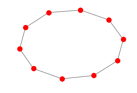
  • Cycle graph with n𝑛n nodes: 𝒞(n)𝒞𝑛\mathcal{C}(n). In our experiments we choose n=10𝑛10n=10. This small simple graph with regular topology is chosen for illustration purposes.

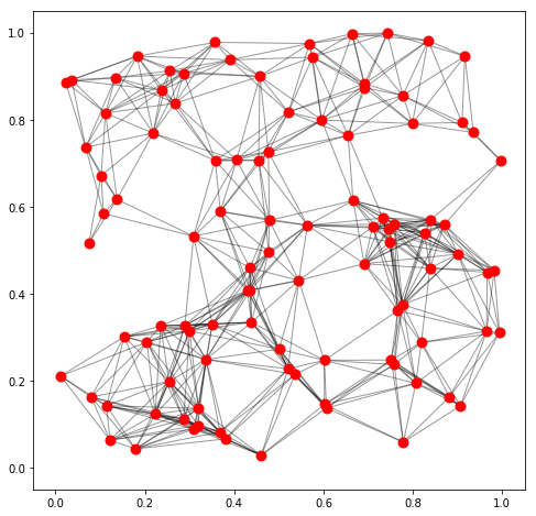
  • Random geometric graph with n𝑛n nodes and radius r𝑟r: 𝒢(n,r)𝒢𝑛𝑟\mathcal{G}(n,r). Random geometric graphs [41] are very important in practice because of their particular formulation which is ideal for modeling wireless sensor networks [26, 5]. In our experiments we focus on a 222-dimensional randomized geometric graph 𝒢(n,r)𝒢𝑛𝑟{\cal G}(n,r) which is formed by placing n𝑛n nodes uniformly at random in a unit square with edges between nodes which are having euclidean distance less than the given radius r𝑟r. We set this to be to be r=r(n)=log(n)/n𝑟𝑟𝑛𝑛𝑛r=r(n)=\sqrt{\log(n)/n} — it is well know that the connectivity is preserved in this case [26]. We set n=100𝑛100n=100.

An illustration of the two graphs appears is in Figure 1.
Refer to caption
(a) Cycle Graph: 𝒞(10)𝒞10{\cal C}(10)
Refer to caption
(b) Random Geometric Graph: 𝒢(n,r)𝒢𝑛𝑟{\cal G}(n,r)
Figure 1: Illustration of the two graph topologies we focus on in this section.

Setup: In all experiments we generate a vector with of initial values cisubscript𝑐𝑖c_{i} from a uniform distribution over [0,1]01[0,1]. We run several experiments and present two kinds of figures that helps us to understand how the algorithms evolve and verify the theoretical results of the previous sections. These figures are:

  1. 1.

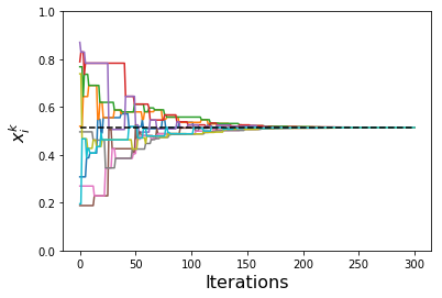
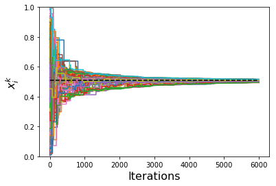
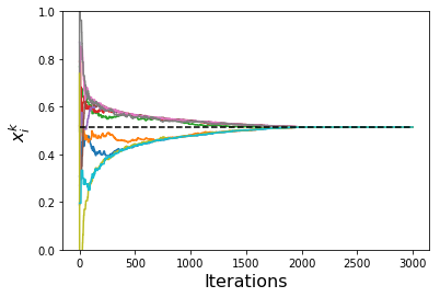
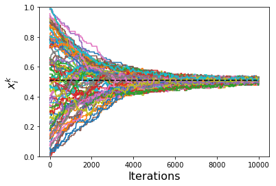
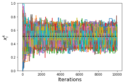
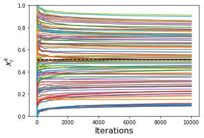
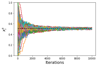
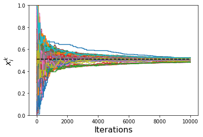
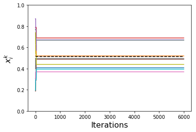
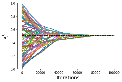
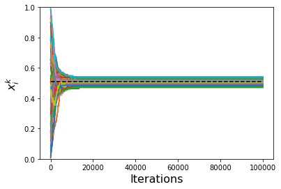
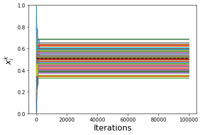
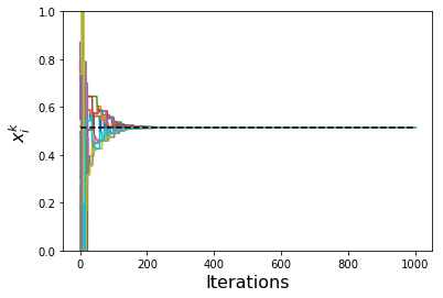
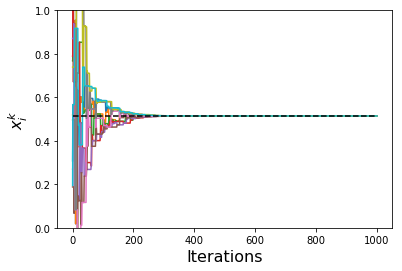
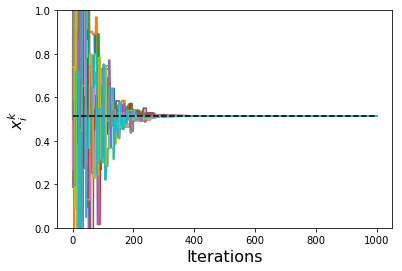
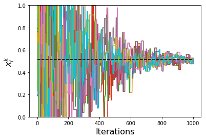
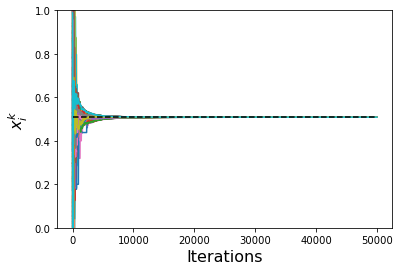
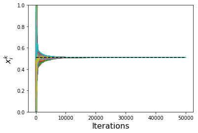
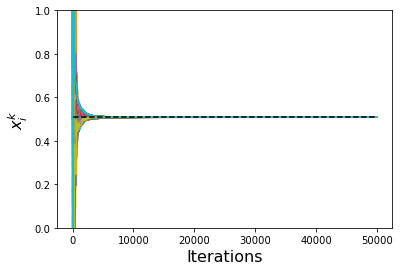
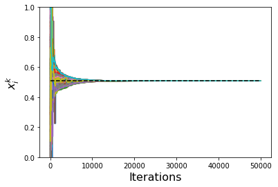
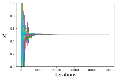
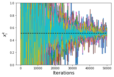
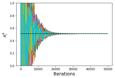
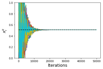
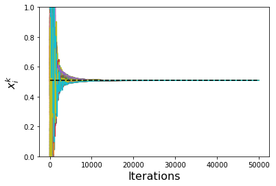
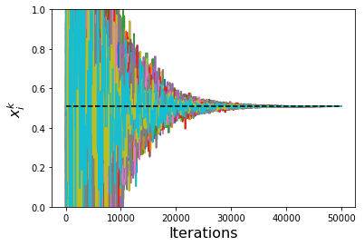
    The evolution of the initial values of the nodes. In these figures we plot how the trajectory of the values xiksuperscriptsubscript𝑥𝑖𝑘x_{i}^{k} of each node i𝑖i evolves throughout iterations. The black doted horizontal line represents the exact average consensus value which all nodes should approach, and thus all other lines should approach this level.

  2. 2.

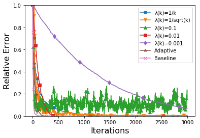
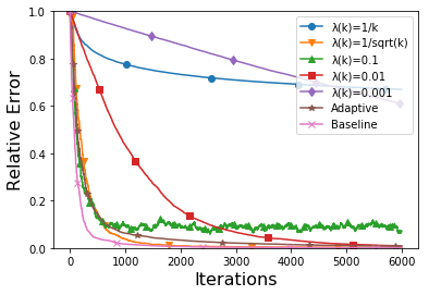
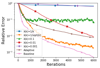
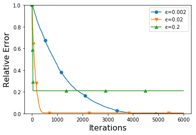
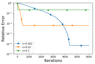
    The evolution of the relative error measure qt=defxtx2x0x2.superscript𝑞𝑡defsuperscriptnormsuperscript𝑥𝑡superscript𝑥2superscriptnormsuperscript𝑥0superscript𝑥2q^{t}\overset{\text{def}}{=}\frac{\|x^{t}-x^{*}\|^{2}}{\|x^{0}-x^{*}\|^{2}}.

We run each method for several parameters and for a pre-specified number of iterations not necessarily the same for each experiment. In each figure we have the relative error, both in normal scale or logarithmic scale, on the vertical axis and number of iterations on the horizontal axis.

To illustrate the first concept, we provide a simple example with the evolution of the initial values xiksuperscriptsubscript𝑥𝑖𝑘x_{i}^{k} for the case of the Standard Gossip algorithm [5] in Figure 2. The horizontal black dotted line represents the average consensus value. It is the exact average of the initial values cisubscript𝑐𝑖c_{i} of the nodes in the network.

Refer to caption
(a) Cycle Graph
Refer to caption
(b) Random Geometric Graph
Figure 2: Trajectories of the values xitsuperscriptsubscript𝑥𝑖𝑡x_{i}^{t} for the Standard Gossip algorithm for Cycle Graph and a random geometric graph. Each line corresponds to xisubscript𝑥𝑖x_{i} for some i𝑖i.

In the rest of this section we evaluate the performance of the novel algorithms we propose, and contrast with the above Standard Gossip algorithm, which we refer to as “Baseline” in the following figures labels.

4.1 Private Gossip via Binary Oracle

In this section we evaluate the performance of Algorithm 2 presented in Section 3.1. In the algorithm, the input parameters are the positive stepsizes {λt}t=0superscriptsubscriptsuperscript𝜆𝑡𝑡0\{\lambda^{t}\}_{t=0}^{\infty}. The goal of the experiments is to compare the performance of the proposed algorithm using different choices of λtsuperscript𝜆𝑡\lambda^{t}.

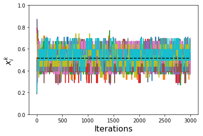
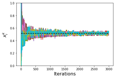
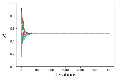
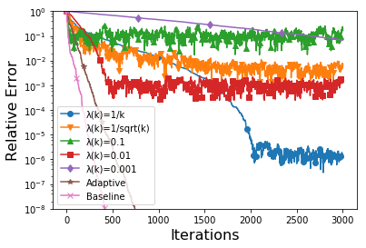
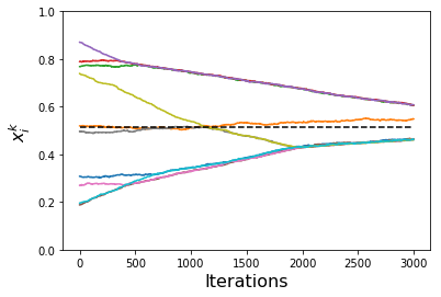
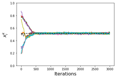
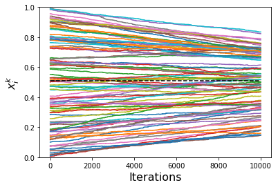
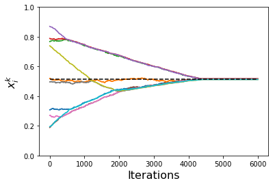
In particular, we use decreasing sequences of stepsizes λt=1/tsuperscript𝜆𝑡1𝑡\lambda^{t}=1/t and λt=1/tsuperscript𝜆𝑡1𝑡\lambda^{t}=1/\sqrt{t}, and three different fixed values for the stepsizes λt=λ{0.001,0.01,0.1}superscript𝜆𝑡𝜆0.0010.010.1\lambda^{t}=\lambda\in\{0.001,0.01,0.1\}. We also include the adaptive choice λt=14me|xitxjt|superscript𝜆𝑡14𝑚subscript𝑒superscriptsubscript𝑥𝑖𝑡superscriptsubscript𝑥𝑗𝑡\lambda^{t}=\frac{1}{4m}\sum_{e\in{\cal E}}|x_{i}^{t}-x_{j}^{t}| which we have proven to converge with linear rate in Theorem 7. We compare these choices in Figures 4 and 6, along with the Standard Gossip algorithm for clear comparison.
Refer to caption
(a) λt=λ=0.001superscript𝜆𝑡𝜆0.001\lambda^{t}=\lambda=0.001
Refer to caption
(b) λt=λ=0.01superscript𝜆𝑡𝜆0.01\lambda^{t}=\lambda=0.01
Refer to caption
(c) λt=λ=0.1superscript𝜆𝑡𝜆0.1\lambda^{t}=\lambda=0.1
Refer to caption
(d) λt=1ksuperscript𝜆𝑡1𝑘\lambda^{t}=\frac{1}{k}
Refer to caption
(e) λt=1ksuperscript𝜆𝑡1𝑘\lambda^{t}=\frac{1}{\sqrt{k}}
Refer to caption
(f) λt=Adaptivesuperscript𝜆𝑡Adaptive\lambda^{t}=\text{Adaptive}
Figure 3: Trajectories of the values of xitsuperscriptsubscript𝑥𝑖𝑡x_{i}^{t} for Binary Oracle run on the cycle graph.
Refer to caption
(a) Linear Scale
Refer to caption
(b) Logarithmic Scale
Figure 4: Convergence of the Binary Oracle run on the cycle graph.

In general, we clearly see what is expected with the constant stepsizes — that they converge to a certain neighbourhood and oscillate around optimum. With smaller stepsize, this neighbourhood is more accurate, but it takes longer to reach. With decreasing stepsizes, Theorem 6 suggests that λtsuperscript𝜆𝑡\lambda^{t} of order 1/t1𝑡1/\sqrt{t} should be optimal. Figure 6 demonstrates this, as the choice of λt=1/tsuperscript𝜆𝑡1𝑡\lambda^{t}=1/t decreases the stepsizes too quickly. However, this is not the case in Figure 4 in which we observe the opposite effect. This is due to the cycle graph being small and simple, and hence the diminishing stepsize becomes problem only after relatively large number of iterations. With the adaptive choice of stepsizes, we recover linear convergence rate as predicted by Theorem 7.

The results in Figure 6 show one surprising comparison. The adaptive choice of stepsizes does not seem to perform better than λt=1/tsuperscript𝜆𝑡1𝑡\lambda^{t}=1/\sqrt{t}. However, we verified that when running for more iterations, the linear rate of adaptive stepsize is present and converges significantly faster to higher accuracies. We chose to present the results for 600060006000 iterations since we found it overall more clean.
Refer to caption
(a) λt=λ=0.001superscript𝜆𝑡𝜆0.001\lambda^{t}=\lambda=0.001
Refer to caption
(b) λt=λ=0.01superscript𝜆𝑡𝜆0.01\lambda^{t}=\lambda=0.01
Refer to caption
(c) λt=λ=0.1superscript𝜆𝑡𝜆0.1\lambda^{t}=\lambda=0.1
Refer to caption
(d) λt=1tsuperscript𝜆𝑡1𝑡\lambda^{t}=\frac{1}{t}
Refer to caption
(e) λt=1tsuperscript𝜆𝑡1𝑡\lambda^{t}=\frac{1}{\sqrt{t}}
Refer to caption
(f) λt=Adaptivesuperscript𝜆𝑡Adaptive\lambda^{t}=\text{Adaptive}
Figure 5: Trajectories of the values of xitsuperscriptsubscript𝑥𝑖𝑡x_{i}^{t} for Binary Oracle run on the random geometric graph.
Refer to caption
(a) Linear Scale
Refer to caption
(b) Logarithmic Scale
Figure 6: Convergence of the Binary Oracle run on the random geometric graph.

4.2 Private Gossip via ϵitalic-ϵ\epsilon-Gap Oracle

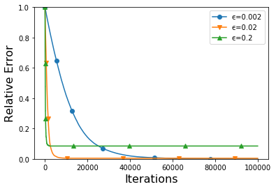
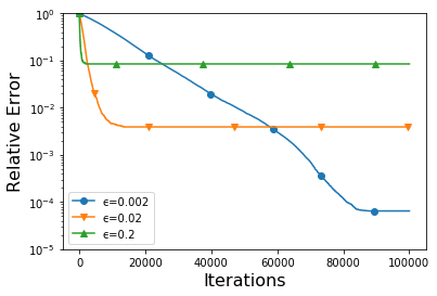
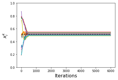
In this section we evaluate the performance of the Algorithm 3 presented in Section 3.2. In the algorithm, the input parameter is the positive error tolerance variable ϵitalic-ϵ\epsilon. For experimental evaluation. we choose three different values for the input, ϵ{0.2,0.02,0.002}italic-ϵ0.20.020.002\epsilon\in\{0.2,0.02,0.002\}, and again use the same cycle and random geometric graphs. The trajectories of the values xitsuperscriptsubscript𝑥𝑖𝑡x_{i}^{t} are presented in Figures 7 and 9, respectively. The performance of the algorithm in terms of the relative error is presented in Figures 8 and 10.

The performance is exactly matching the expectation — with larger ϵitalic-ϵ\epsilon, the method converges very fast to a wide neighbourhood of the optimum. For a small value, it converges much closer to the optimum, but it requires more iterations.
Refer to caption
(a) ϵ=0.002italic-ϵ0.002\epsilon=0.002
Refer to caption
(b) ϵ=0.02italic-ϵ0.02\epsilon=0.02
Refer to caption
(c) ϵ=0.2italic-ϵ0.2\epsilon=0.2
Figure 7: Trajectories of the values of xitsuperscriptsubscript𝑥𝑖𝑡x_{i}^{t} for ϵitalic-ϵ\epsilon-Gap Oracle run on the cycle graph.
Refer to caption
(a) Linear Scale
Refer to caption
(b) Logarithmic Scale
Figure 8: Convergence of the ϵitalic-ϵ\epsilon-Gap Oracle run on the cycle graph.
Refer to caption
(a) ϵ=0.002italic-ϵ0.002\epsilon=0.002
Refer to caption
(b) ϵ=0.02italic-ϵ0.02\epsilon=0.02
Refer to caption
(c) ϵ=0.2italic-ϵ0.2\epsilon=0.2
Figure 9: Trajectories of the values of xitsuperscriptsubscript𝑥𝑖𝑡x_{i}^{t} for ϵitalic-ϵ\epsilon-Gap Oracle run on the random geometric graph.
Refer to caption
(a) Linear Scale
Refer to caption
(b) Logarithmic Scale
Figure 10: Convergence of the ϵitalic-ϵ\epsilon-Gap Oracle run on the random geometric graph.

4.3 Private Gossip via Controlled Noise Insertion

In this section we evaluate the performance of Algorithm 4 presented in Section 3.3. This algorithm has two different parameters for each node i𝑖i. These are the initial variance σi20superscriptsubscript𝜎𝑖20\sigma_{i}^{2}\geq 0 and the rate of decay, ϕisubscriptitalic-ϕ𝑖\phi_{i}, of the noise.

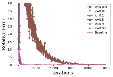
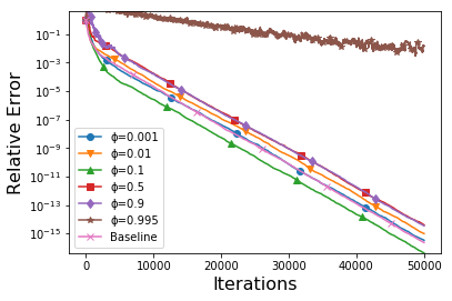
To evaluate the impact of these parameters, we perform several experiments. As earlier, we use the same graph structures for evaluation: cycle graph and random geometric graph. The algorithm converges with a linear rate depending on maximum of two factors — see Theorem 11 and Corollary 12. We will verify that this is indeed the case, and for values of ϕisubscriptitalic-ϕ𝑖\phi_{i} above a certain threshold, the convergence is driven by the rate at which the noise decays. This is true for both identical values of ϕisubscriptitalic-ϕ𝑖\phi_{i} for all i𝑖i, and for varying values as per (20). We further demonstrate the latter is superior in the sense that it enables insertion of more noise, without sacrificing the convergence speed. Finally, we study the effect of various magnitudes of the noise inserted initially.

4.3.1 Fixed variance, identical decay rates

In this part, we run Algorithm 4 with σi=1subscript𝜎𝑖1\sigma_{i}=1 for all i𝑖i, and set ϕi=ϕsubscriptitalic-ϕ𝑖italic-ϕ\phi_{i}=\phi for all i𝑖i and some ϕitalic-ϕ\phi. We study the effect of varying the value of ϕitalic-ϕ\phi on the convergence of the algorithm.

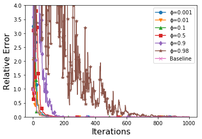
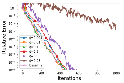
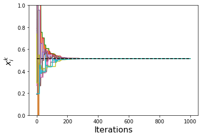
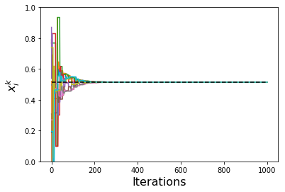
In both Figures 12b and 14b, we see that for small values of ϕitalic-ϕ\phi, we eventually recover the same rate of linear convergence as the Standard Gossip algorithm. If the value of ϕitalic-ϕ\phi is sufficiently close to 111 however, the rate is driven by the noise and not by the convergence of the Standard Gossip algorithm. This value is ϕ=0.98italic-ϕ0.98\phi=0.98 for cycle graph, and ϕ=0.995italic-ϕ0.995\phi=0.995 for the random geometric graph in the plots we present.

Looking at the individual runs for small values of ϕitalic-ϕ\phi in Figure 14b, we see some variance in terms of when the asymptotic rate is realized. We would like to point out that this does not provide additional insight into whether specific small values of ϕitalic-ϕ\phi are in general better for the following reason. The Standard Gossip algorithm is itself a randomized algorithm, with an inherent uncertainty in the convergence of any particular run. If we ran the algorithms multiple times, we observe variance in the evolution of the suboptimality of similar magnitude, just as what we see in the figure. Hence, the variance is expected, and not significantly influenced by the noise.
Refer to caption
(a) ϕ=0.001italic-ϕ0.001\phi=0.001
Refer to caption
(b) ϕ=0.01italic-ϕ0.01\phi=0.01
Refer to caption
(c) ϕ=0.1italic-ϕ0.1\phi=0.1
Refer to caption
(d) ϕ=0.5italic-ϕ0.5\phi=0.5
Refer to caption
(e) ϕ=0.9italic-ϕ0.9\phi=0.9
Refer to caption
(f) ϕ=0.98italic-ϕ0.98\phi=0.98
Figure 11: Trajectories of the values of xitsuperscriptsubscript𝑥𝑖𝑡x_{i}^{t} for Controlled Noise Insertion run on the cycle graph for different values of ϕitalic-ϕ\phi.
Refer to caption
(a) Linear Scale
Refer to caption
(b) Logarithmic Scale
Figure 12: Convergence of the Controlled Noise Insertion run on the cycle graph for different values of ϕitalic-ϕ\phi.
Refer to caption
(a) ϕ=0.001italic-ϕ0.001\phi=0.001
Refer to caption
(b) ϕ=0.01italic-ϕ0.01\phi=0.01
Refer to caption
(c) ϕ=0.1italic-ϕ0.1\phi=0.1
Refer to caption
(d) ϕ=0.5italic-ϕ0.5\phi=0.5
Refer to caption
(e) ϕ=0.9italic-ϕ0.9\phi=0.9
Refer to caption
(f) ϕ=0.995italic-ϕ0.995\phi=0.995
Figure 13: Trajectories of the values of xitsuperscriptsubscript𝑥𝑖𝑡x_{i}^{t} for Controlled Noise Insertion run on the random geometric graph for different values of ϕitalic-ϕ\phi.
Refer to caption
(a) Linear Scale
Refer to caption
(b) Logarithmic Scale
Figure 14: Convergence of the Controlled Noise Insertion run on the random geometric graph for different values of ϕitalic-ϕ\phi.

4.3.2 Variance 1 and different decay rates

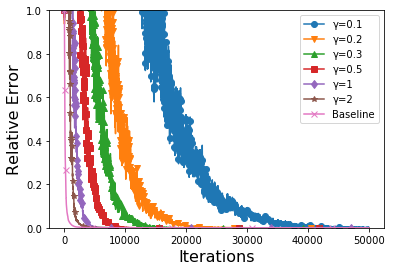
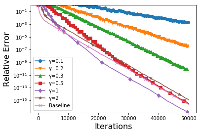
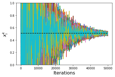
In this section, we perform similar experiment as above, but let the values ϕisubscriptitalic-ϕ𝑖\phi_{i} be vary for different nodes i𝑖i. This is controlled by the choice of γ𝛾\gamma as in (20). Note that by decreasing γ𝛾\gamma, we increase ϕisubscriptitalic-ϕ𝑖\phi_{i}, and thus smaller γ𝛾\gamma means the noise decays at a slower rate. Here, due to the regular structure of the cycle graph, we present only results for the random geometric graph.

It is not straightforward to compare this setting with the setting of identical ϕisubscriptitalic-ϕ𝑖\phi_{i}, and we return to it in the next section. Here we only remark that we again see the existence of a threshold predicted by theory, beyond which the convergence is dominated by the inserted noise. Otherwise, we recover the rate of the Standard Gossip algorithm.
Refer to caption
(a) γ=0.1𝛾0.1\gamma=0.1
Refer to caption
(b) γ=0.2𝛾0.2\gamma=0.2
Refer to caption
(c) γ=0.3𝛾0.3\gamma=0.3
Refer to caption
(d) γ=0.5𝛾0.5\gamma=0.5
Refer to caption
(e) γ=1𝛾1\gamma=1
Refer to caption
(f) γ=2𝛾2\gamma=2
Figure 15: Trajectories of the values of xitsuperscriptsubscript𝑥𝑖𝑡x_{i}^{t} for Controlled Noise Insertion run on the random geometric graph for different values of ϕisubscriptitalic-ϕ𝑖\phi_{i}, controlled by γ𝛾\gamma.
Refer to caption
(a) Normal Scale
Refer to caption
(b) Logarithmic Scale
Figure 16: Convergence of the Controlled Noise Insertion run on the random geometric graph for different values of ϕisubscriptitalic-ϕ𝑖\phi_{i}, controlled by γ𝛾\gamma.

4.3.3 Impact of varying ϕisubscriptitalic-ϕ𝑖\phi_{i}

In this experiment, we demonstrate the practical utility of letting the rate of decay ϕisubscriptitalic-ϕ𝑖\phi_{i} to be different on each node i𝑖i. In order to do so, we run experiment on the random geometric graph and compare the settings investigated in the previous two sections — the noise decay rate driven by ϕitalic-ϕ\phi, or by γ𝛾\gamma.

In first place, we choose the values of ϕisubscriptitalic-ϕ𝑖\phi_{i} such that that the two factors in Corollary 12 are equal. For the particular graph we used, this corresponds to γ0.17𝛾0.17\gamma\approx 0.17 with ϕi=1α(𝒢)2disubscriptitalic-ϕ𝑖1𝛼𝒢2subscript𝑑𝑖\phi_{i}=\sqrt{1-\frac{\alpha({\cal G})}{2d_{i}}}. Second, we make the factors equal, but with constraint of having ϕisubscriptitalic-ϕ𝑖\phi_{i} to be equal for all i𝑖i. This corresponds to ϕi0.983subscriptitalic-ϕ𝑖0.983\phi_{i}\approx 0.983 for all i𝑖i.

The performance for a large number of iterations is displayed in left side of Figure 17. We see that theabove two choices indeed yield very similar practical performance, which also eventually matches the rate predicted by theory. For complete comparison, we also include performance of the Standard Gossip algorithm.
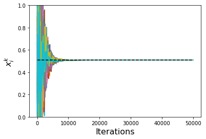
The important message is conveyed in the histogram in the right side of Figure 17. The histogram shows the distribution of the values of ϕisubscriptitalic-ϕ𝑖\phi_{i} for different nodes i𝑖i. The minimum of these values is what we needed in the case of identical ϕisubscriptitalic-ϕ𝑖\phi_{i} for all i𝑖i. However, most of the values are significantly higher. This means, that if we allow the noise decay rates to depend on the number of neighbours, we are able to increase the amount of noise inserted, without sacrificing practical performance. This is beneficial, as more noise will likely be beneficial for any formal notion of protection of the initial values.
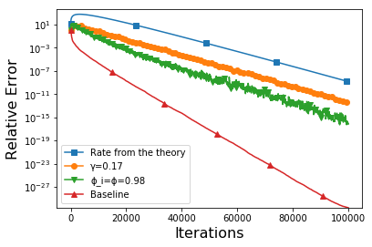
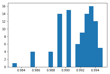
Refer to caption
Refer to caption
Figure 17: Left: Performance of the noise oracle with noise decrease rate chosen according to Corollary 12. Right: Histogram of of distribution of ϕisubscriptitalic-ϕ𝑖\phi_{i}

5 Conclusion

In this work we addressed the Average Consensus problem via novel asynchronous randomized gossip algorithms. We propose algorithmic tools for protection of the private values each node in the network holds initially. However, we do not quantify any formal notion of privacy protection achievable using these tools; this is left for future research.

In particular, we propose two ways to achieve this goal. First, which we believe is the first of its kind, weakens the oracle used in the gossip framework, to provide only categorical (or even binary) information to each participating node about the value of the other node. In the second approach, we systematically inject and withdraw noise throughout the iterations, so as to ensure convergence to the average consensus value. In all cases, we provide explicit convergence rates and evaluate practical convergence on common simulated network topologies.

References

  • [1] Zeyuan Allen-Zhu, Zheng Qu, Peter Richtárik, and Yang Yuan. Even faster accelerated coordinate descent using non-uniform sampling. In Proceedings of The 33rd International Conference on Machine Learning, pages 1110–1119, 2016.
  • [2] Tuncer Can Aysal, Mehmet Ercan Yildiz, Anand D Sarwate, and Anna Scaglione. Broadcast gossip algorithms for consensus. IEEE Transactions on Signal processing, 57(7):2748–2761, 2009.
  • [3] Florence Bénézit, Alexandros G Dimakis, Patrick Thiran, and Martin Vetterli. Order-optimal consensus through randomized path averaging. IEEE Transactions on Information Theory, 56(10):5150–5167, 2010.
  • [4] Dimitri P Bertsekas and John N Tsitsiklis. Parallel and distributed computation: numerical methods, volume 23. Prentice hall Englewood Cliffs, NJ, 1989.
  • [5] Stephen Boyd, Arpita Ghosh, Balaji Prabhakar, and Devavrat Shah. Randomized gossip algorithms. IEEE Transactions on Information Theory, 14(SI):2508–2530, 2006.
  • [6] Ming Cao, Daniel A Spielman, and Edmund M Yeh. Accelerated gossip algorithms for distributed computation. In Proceedings of the 44th Annual Allerton Conference on Communication, Control, and Computation, pages 952–959, 2006.
  • [7] Antonin Chambolle, Matthias J. Ehrhardt, Peter Richtárik, and Carola-Bibiane Schoenlieb. Stochastic primal-dual hybrid gradient algorithm with arbitrary sampling and imaging applications. arXiv:1706.04957, 2017.
  • [8] Ronald Cramer, Ivan Bjerre Damgård, and Jesper Buus Nielsen. Secure Multiparty Computation and Secret Sharing. Cambridge University Press, 2015.
  • [9] Dominik Csiba, Zheng Qu, and Peter Richtárik. Stochastic Dual Coordinate Ascent with Adaptive Probabilities. ICML 2015, 2015.
  • [10] George Cybenko. Dynamic load balancing for distributed memory multiprocessors. Journal of Parallel and Distributed Computing, 7(2):279–301, 1989.
  • [11] Alexandros DG Dimakis, Anand D Sarwate, and Martin J Wainwright. Geographic gossip: Efficient averaging for sensor networks. IEEE Transactions on Signal Processing, 56(3):1205–1216, 2008.
  • [12] Alexandros G Dimakis, Soummya Kar, José MF Moura, Michael G Rabbat, and Anna Scaglione. Gossip algorithms for distributed signal processing. Proceedings of the IEEE, 98(11):1847–1864, 2010.
  • [13] Cynthia Dwork, Aaron Roth, et al. The algorithmic foundations of differential privacy. Foundations and Trends® in Theoretical Computer Science, 9(3–4):211–407, 2014.
  • [14] Olivier Fercoq and Peter Richtárik. Smooth minimization of nonsmooth functions by parallel coordinate descent. arXiv:1309.5885, 2013.
  • [15] Olivier Fercoq and Peter Richtárik. Accelerated, parallel and proximal coordinate descent. SIAM Journal on Optimization, (25):1997–2023, 2015.
  • [16] Miroslav Fiedler. Algebraic connectivity of graphs. Czechoslovak mathematical journal, 23(2):298–305, 1973.
  • [17] Mauro Franceschelli, Alessandro Giua, and Carla Seatzu. Distributed averaging in sensor networks based on broadcast gossip algorithms. IEEE Sensors Journal, 11(3):808–817, 2011.
  • [18] Nikolaos M Freris and Anastasios Zouzias. Fast distributed smoothing of relative measurements. In IEEE 51st Annual Conference on Decision and Control (CDC), pages 1411–1416. IEEE, 2012.
  • [19] Valerio Freschi, Emanuele Lattanzi, and Alessandro Bogliolo. Accelerating distributed averaging in sensor networks: Randomized gossip over virtual coordinates. In Sensors Applications Symposium (SAS), 2016 IEEE, pages 1–6. IEEE, 2016.
  • [20] Valerio Freschi, Emanuele Lattanzi, and Alessandro Bogliolo. Fast distributed consensus through path averaging on random walks. Wireless Pers Commun, doi:10.1007/s11277-017-4451-5:1–15, 2017.
  • [21] Robert Mansel Gower, Donald Goldfarb, and Peter Richtárik. Stochastic block BFGS: squeezing more curvature out of data. In Proceedings of The 33rd International Conference on Machine Learning, pages 1869–1878, 2016.
  • [22] Robert Mansel Gower and Peter Richtárik. Randomized iterative methods for linear systems. SIAM Journal on Matrix Analysis and Applications, 36(4):1660–1690, 2015.
  • [23] Robert Mansel Gower and Peter Richtárik. Stochastic dual ascent for solving linear systems. arXiv:1512.06890, 2015.
  • [24] Robert Mansel Gower and Peter Richtárik. Linearly convergent randomized iterative methods for computing the pseudoinverse. arXiv preprint arXiv:1612.06255, 2016.
  • [25] Robert Mansel Gower and Peter Richtárik. Randomized quasi-Newton updates are linearly convergent matrix inversion algorithms. arXiv preprint arXiv:1602.01768, 2016.
  • [26] Piyush Gupta and Panganmala R Kumar. The capacity of wireless networks. IEEE Transactions on Information Theory, 46(2):388–404, 2000.
  • [27] Fenghua He, A Stephen Morse, Ji Liu, and Shaoshuai Mou. Periodic gossiping. IFAC Proceedings Volumes, 44(1):8718–8723, 2011.
  • [28] Zhenqi Huang, Sayan Mitra, and Geir Dullerud. Differentially private iterative synchronous consensus. In Proceedings of the 2012 ACM workshop on Privacy in the electronic society, pages 81–90. ACM, 2012.
  • [29] Ye Yu Jun and Michael Rabbat. Performance comparison of randomized gossip, broadcast gossip and collection tree protocol for distributed averaging. In IEEE 5th International Workshop on Computational Advances in Multi-Sensor Adaptive Processing (CAMSAP), pages 93–96. IEEE, 2013.
  • [30] David Kempe, Alin Dobra, and Johannes Gehrke. Gossip-based computation of aggregate information. In Foundations of Computer Science, 2003. Proceedings. 44th Annual IEEE Symposium on, pages 482–491. IEEE, 2003.
  • [31] Yin Tat Lee and Aaron Sidford. Efficient accelerated coordinate descent methods and faster algorithms for solving linear systems. In Foundations of Computer Science (FOCS), 2013 IEEE 54th Annual Symposium on, pages 147–156. IEEE, 2013.
  • [32] Dennis Leventhal and Adrian S. Lewis. Randomized methods for linear constraints: Convergence rates and conditioning. Mathematics of Operations Research, 35(3):641–654, 2010.
  • [33] Ji Liu, Brian D.O. Anderson, Ming Cao, and A Stephen Morse. Analysis of accelerated gossip algorithms. Automatica, 49(4):873–883, 2013.
  • [34] Ji Liu, Shaoshuai Mou, A Stephen Morse, Brian DO Anderson, and Changbin Yu. Deterministic gossiping. Proceedings of the IEEE, 99(9):1505–1524, 2011.
  • [35] Nicolas Loizou and Peter Richtárik. A new perspective on randomized gossip algorithms. In 4th IEEE Global Conference on Signal and Information Processing (GlobalSIP), 2016.
  • [36] Nicolaos E Manitara and Christoforos N Hadjicostis. Privacy-preserving asymptotic average consensus. In Control Conference (ECC), 2013 European, pages 760–765. IEEE, 2013.
  • [37] Yilin Mo and Richard M Murray. Privacy preserving average consensus. IEEE Transactions on Automatic Control, 62(2):753–765, 2017.
  • [38] Shaoshuai Mou, Changbin Yu, Brian DO Anderson, and A Stephen Morse. Deterministic gossiping with a periodic protocol. In Decision and Control (CDC), 2010 49th IEEE Conference on, pages 5787–5791. IEEE, 2010.
  • [39] Yurii Nesterov. Efficiency of coordinate descent methods on huge-scale optimization problems. SIAM Journal on Optimization, 22(2):341–362, 2012.
  • [40] Reza Olfati-Saber, J Alex Fax, and Richard M Murray. Consensus and cooperation in networked multi-agent systems. Proceedings of the IEEE, 95(1):215–233, 2007.
  • [41] Mathew Penrose. Random geometric graphs. Number 5. Oxford University Press, 2003.
  • [42] Zheng Qu and Richtárik. Coordinate descent with arbitrary sampling I: algorithms and complexity. Optimization Methods and Software, 31(5):829–857, 2016.
  • [43] Zheng Qu and Richtárik. Coordinate descent with arbitrary sampling II: expected separable overapproximation. Optimization Methods and Software, 31(5):858–884, 2016.
  • [44] Zheng Qu, Peter Richtárik, and Tong Zhang. Quartz: Randomized dual coordinate ascent with arbitrary sampling. In Advances in Neural Information Processing Systems 28, 2015.
  • [45] Wei Ren, Randal W Beard, and Ella M Atkins. Information consensus in multivehicle cooperative control. IEEE Control Systems, 27(2):71–82, 2007.
  • [46] Peter Richtárik and Martin Takáč. Iteration complexity of randomized block-coordinate descent methods for minimizing a composite function. Mathematical Programming, 144(2):1–38, 2014.
  • [47] Peter Richtárik and Martin Takáč. Parallel coordinate descent methods for big data optimization. Mathematical Programming, 156(1):433–484, 2016.
  • [48] Peter Richtárik and Martin Takáč. Stochastic reformulations of linear systems: algorithms and convergence theory. arXiv preprint arXiv:1706.01108, 2017.
  • [49] Devavrat Shah. Gossip algorithms. Foundations and Trends® in Networking, 3(1):1–125, 2009.
  • [50] Shai Shalev-Shwartz and Tong Zhang. Stochastic Dual Coordinate Ascent Methods for Regularized Loss Minimization. Journal of Machine Learning Research, 14:567–599, 2012.
  • [51] John Tsitsiklis, Dimitri Bertsekas, and Michael Athans. Distributed asynchronous deterministic and stochastic gradient optimization algorithms. IEEE transactions on automatic control, 31(9):803–812, 1986.
  • [52] John Nikolas Tsitsiklis. Problems in decentralized decision making and computation. Technical report, DTIC Document, 1984.
  • [53] Shaochuan Wu and Michael G Rabbat. Broadcast gossip algorithms for consensus on strongly connected digraphs. IEEE Transactions on Signal Processing, 61(16):3959–3971, 2013.
  • [54] Lin Xiao and Stephen Boyd. Fast linear iterations for distributed averaging. Systems & Control Letters, 53(1):65–78, 2004.
  • [55] Lin Xiao, Stephen Boyd, and Sanjay Lall. A scheme for robust distributed sensor fusion based on average consensus. In Proceedings of the 4th international symposium on Information processing in sensor networks, page 9. IEEE Press, 2005.
  • [56] Changbin Brad Yu, Brian DO Anderson, Shaoshuai Mou, Ji Liu, Fenghua He, and A Stephen Morse. Distributed averaging using periodic gossiping. IEEE Transactions on Automatic Control, 2017.

Appendix A Proofs for Section 1

A.1 Proof of Lemma 1

Lemma 13.
i=1n(j=1n(xjxi))2=n2i=1nj=1n(xjxi)2superscriptsubscript𝑖1𝑛superscriptsuperscriptsubscript𝑗1𝑛subscript𝑥𝑗subscript𝑥𝑖2𝑛2superscriptsubscript𝑖1𝑛superscriptsubscript𝑗1𝑛superscriptsubscript𝑥𝑗subscript𝑥𝑖2\sum_{i=1}^{n}\left(\sum_{j=1}^{n}(x_{j}-x_{i})\right)^{2}=\frac{n}{2}\sum_{i=1}^{n}\sum_{j=1}^{n}(x_{j}-x_{i})^{2} (21)
Proof.

Using simple algebra we have

i=1n(j=1n(xjxi))2superscriptsubscript𝑖1𝑛superscriptsuperscriptsubscript𝑗1𝑛subscript𝑥𝑗subscript𝑥𝑖2\displaystyle\sum_{i=1}^{n}\left(\sum_{j=1}^{n}(x_{j}-x_{i})\right)^{2} =\displaystyle= i=1n(j=1nxjnxi)2superscriptsubscript𝑖1𝑛superscriptsuperscriptsubscript𝑗1𝑛subscript𝑥𝑗𝑛subscript𝑥𝑖2\displaystyle\sum_{i=1}^{n}\left(\sum_{j=1}^{n}x_{j}-nx_{i}\right)^{2}
=\displaystyle= i=1n((j=1nxj)2+n2xi22nxi(j=1nxj))superscriptsubscript𝑖1𝑛superscriptsuperscriptsubscript𝑗1𝑛subscript𝑥𝑗2superscript𝑛2superscriptsubscript𝑥𝑖22𝑛subscript𝑥𝑖superscriptsubscript𝑗1𝑛subscript𝑥𝑗\displaystyle\sum_{i=1}^{n}\left(\left(\sum_{j=1}^{n}x_{j}\right)^{2}+n^{2}x_{i}^{2}-2nx_{i}\left(\sum_{j=1}^{n}x_{j}\right)\right)
=\displaystyle= n(j=1nxj)2+n2i=1nxi22n(j=1nxj)2𝑛superscriptsuperscriptsubscript𝑗1𝑛subscript𝑥𝑗2superscript𝑛2superscriptsubscript𝑖1𝑛superscriptsubscript𝑥𝑖22𝑛superscriptsuperscriptsubscript𝑗1𝑛subscript𝑥𝑗2\displaystyle n\left(\sum_{j=1}^{n}x_{j}\right)^{2}+n^{2}\sum_{i=1}^{n}x_{i}^{2}-2n\left(\sum_{j=1}^{n}x_{j}\right)^{2}
=\displaystyle= n2i=1nxi2n(i=1nxi)2.superscript𝑛2superscriptsubscript𝑖1𝑛superscriptsubscript𝑥𝑖2𝑛superscriptsuperscriptsubscript𝑖1𝑛subscript𝑥𝑖2\displaystyle n^{2}\sum_{i=1}^{n}x_{i}^{2}-n\left(\sum_{i=1}^{n}x_{i}\right)^{2}.

Manipulating right hand side of (21) we obtain

n2i=1nj=1n(xjxi)2𝑛2superscriptsubscript𝑖1𝑛superscriptsubscript𝑗1𝑛superscriptsubscript𝑥𝑗subscript𝑥𝑖2\displaystyle\frac{n}{2}\sum_{i=1}^{n}\sum_{j=1}^{n}(x_{j}-x_{i})^{2} =\displaystyle= n2i=1nj=1n(xj2+xi22xixj)𝑛2superscriptsubscript𝑖1𝑛superscriptsubscript𝑗1𝑛superscriptsubscript𝑥𝑗2superscriptsubscript𝑥𝑖22subscript𝑥𝑖subscript𝑥𝑗\displaystyle\frac{n}{2}\sum_{i=1}^{n}\sum_{j=1}^{n}\left(x_{j}^{2}+x_{i}^{2}-2x_{i}x_{j}\right)
=\displaystyle= n2i=1nxi2ni=1nj=1nxixj=n2i=1nxi2n(i=1nxi)2.superscript𝑛2superscriptsubscript𝑖1𝑛superscriptsubscript𝑥𝑖2𝑛superscriptsubscript𝑖1𝑛superscriptsubscript𝑗1𝑛subscript𝑥𝑖subscript𝑥𝑗superscript𝑛2superscriptsubscript𝑖1𝑛superscriptsubscript𝑥𝑖2𝑛superscriptsuperscriptsubscript𝑖1𝑛subscript𝑥𝑖2\displaystyle n^{2}\sum_{i=1}^{n}x_{i}^{2}-n\sum_{i=1}^{n}\sum_{j=1}^{n}x_{i}x_{j}\quad=\quad n^{2}\sum_{i=1}^{n}x_{i}^{2}-n\left(\sum_{i=1}^{n}x_{i}\right)^{2}.

Clearly, LHS and RHS of (21) are equal.

In order to show (2) it is enough to notice that

c¯𝟏x2superscriptnorm¯𝑐1𝑥2\displaystyle\|\bar{c}{\bf 1}-x\|^{2} =\displaystyle= i=1n(c¯xi)2=i=1n(1nj=1nxjxi)2superscriptsubscript𝑖1𝑛superscript¯𝑐subscript𝑥𝑖2superscriptsubscript𝑖1𝑛superscript1𝑛superscriptsubscript𝑗1𝑛subscript𝑥𝑗subscript𝑥𝑖2\displaystyle\sum_{i=1}^{n}(\bar{c}-x_{i})^{2}\quad=\quad\sum_{i=1}^{n}\left(\frac{1}{n}\sum_{j=1}^{n}x_{j}-x_{i}\right)^{2}
=\displaystyle= i=1n(j=1n1n(xjxi))2=(21)12i=1nj=1n1n(xjxi)2superscriptsubscript𝑖1𝑛superscriptsuperscriptsubscript𝑗1𝑛1𝑛subscript𝑥𝑗subscript𝑥𝑖2italic-(21italic-)12superscriptsubscript𝑖1𝑛superscriptsubscript𝑗1𝑛1𝑛superscriptsubscript𝑥𝑗subscript𝑥𝑖2\displaystyle\sum_{i=1}^{n}\left(\sum_{j=1}^{n}\frac{1}{n}(x_{j}-x_{i})\right)^{2}\quad\overset{\eqref{Eq: sum lemma}}{=}\quad\frac{1}{2}\sum_{i=1}^{n}\sum_{j=1}^{n}\frac{1}{n}(x_{j}-x_{i})^{2}
=\displaystyle= 12ni=1nj=1n(xjxi)2.12𝑛superscriptsubscript𝑖1𝑛superscriptsubscript𝑗1𝑛superscriptsubscript𝑥𝑗subscript𝑥𝑖2\displaystyle\frac{1}{2n}\sum_{i=1}^{n}\sum_{j=1}^{n}(x_{j}-x_{i})^{2}.

Note that we have

1nm(e=(i,j)|xixj|)21ne(xixj)21n(i,j)(xixj)2=(2)c¯𝟏x2,1𝑛𝑚superscriptsubscript𝑒𝑖𝑗subscript𝑥𝑖subscript𝑥𝑗21𝑛subscript𝑒superscriptsubscript𝑥𝑖subscript𝑥𝑗21𝑛subscript𝑖𝑗superscriptsubscript𝑥𝑖subscript𝑥𝑗2superscriptitalic-(2italic-)superscriptnorm¯𝑐1𝑥2\frac{1}{nm}\left(\sum_{e=(i,j)\in{\cal E}}|x_{i}-x_{j}|\right)^{2}\leq\frac{1}{n}\sum_{e\in{\cal E}}(x_{i}-x_{j})^{2}\leq\frac{1}{n}\sum_{(i,j)}(x_{i}-x_{j})^{2}\stackrel{{\scriptstyle\eqref{Eq: equality}}}{{=}}\|\bar{c}{\bf 1}-x\|^{2},

which proves (3). On the other hand, we have

1α(𝒢)(e=(i,j)|xixj|)21α(𝒢)e(xixj)2(23)c¯𝟏x2,1𝛼𝒢superscriptsubscript𝑒𝑖𝑗subscript𝑥𝑖subscript𝑥𝑗21𝛼𝒢subscript𝑒superscriptsubscript𝑥𝑖subscript𝑥𝑗2superscriptitalic-(23italic-)superscriptnorm¯𝑐1𝑥2\frac{1}{\alpha({\cal G})}\left(\sum_{e=(i,j)\in{\cal E}}|x_{i}-x_{j}|\right)^{2}\geq\frac{1}{\alpha({\cal G})}\sum_{e\in{\cal E}}\left(x_{i}-x_{j}\right)^{2}\stackrel{{\scriptstyle\eqref{eq:8998gd98gikd}}}{{\geq}}\|\bar{c}{\bf 1}-x\|^{2},

which concludes (4). Inequality (5) holds trivially.

Appendix B Proofs for Section 2.4

We now perform the analysis of Algorithm 1.

B.1 Proof of Lemma 4

Lemma 14.

The eigenvalues of 𝐋~=n𝐈𝟏𝟏~𝐋𝑛𝐈superscript11top\tilde{{\bf L}}=n{\bf I}-{\bf 1}{\bf 1}^{\top} are {0,n,n,,n}0𝑛𝑛𝑛\{0,n,n,\dots,n\}

Proof.

Clearly, 𝐋~𝟏=0~𝐋10\tilde{{\bf L}}{\bf 1}=0. Consider some vector x𝑥x such that x,𝟏=0𝑥10\langle x,{\bf 1}\rangle=0. Then, 𝐋~x=n𝐈x𝟏𝟏x=nx+𝟏𝟏x=nx~𝐋𝑥𝑛𝐈𝑥superscript11top𝑥𝑛𝑥superscript11top𝑥𝑛𝑥\tilde{{\bf L}}x=n{\bf I}x-{\bf 1}{\bf 1}^{\top}x=nx+{\bf 1}{\bf 1}^{\top}x=nx thus x𝑥x is an eigenvector corresponding to eigenvalue n𝑛n. Thus, we can pick n1𝑛1n-1 linearly independent eigenvectors of 𝐋~~𝐋\tilde{{\bf L}} corresponding to eigenvalue n𝑛n, which concludes the proof. ∎

The Laplacian matrix of 𝒢𝒢{\cal G} is the matrix 𝐋=𝐀𝐀𝐋superscript𝐀top𝐀{\bf L}={\bf A}^{\top}{\bf A}. We have 𝐋ii=disubscript𝐋𝑖𝑖subscript𝑑𝑖{\bf L}_{ii}=d_{i} (degree of vertex i𝑖i), 𝐋ij=𝐋ji=1subscript𝐋𝑖𝑗subscript𝐋𝑗𝑖1{\bf L}_{ij}={\bf L}_{ji}=-1 if (i,j)𝑖𝑗(i,j)\in{\cal E} and 𝐋ij=0subscript𝐋𝑖𝑗0{\bf L}_{ij}=0 otherwise. A simple computation reveals that for any xn𝑥superscript𝑛x\in\mathbb{R}^{n} we have

x𝐋x=e=(i,j)(xixj)2.superscript𝑥top𝐋𝑥subscript𝑒𝑖𝑗superscriptsubscript𝑥𝑖subscript𝑥𝑗2x^{\top}{\bf L}x=\sum_{e=(i,j)\in{\cal E}}(x_{i}-x_{j})^{2}.

Let 𝐀~~𝐀\tilde{{\bf A}} be the n(n1)/2×n𝑛𝑛12𝑛n(n-1)/2\times n matrix corresponding to the complete graph 𝒢~~𝒢\tilde{{\cal G}} on 𝒱𝒱{\cal V}. Let 𝐋~=𝐀~𝐀~~𝐋superscript~𝐀top~𝐀\tilde{{\bf L}}=\tilde{{\bf A}}^{\top}\tilde{{\bf A}} be its Laplacian. We have 𝐋~ii=n1subscript~𝐋𝑖𝑖𝑛1\tilde{{\bf L}}_{ii}=n-1 for all i𝑖i and 𝐋~ij=1subscript~𝐋𝑖𝑗1\tilde{{\bf L}}_{ij}=-1 for ij𝑖𝑗i\neq j. So, 𝐋~=n𝐈𝟏𝟏~𝐋𝑛𝐈superscript11top\tilde{{\bf L}}=n{\bf I}-{\bf 1}{\bf 1}^{\top}. Then

x𝐋~x=nx2(i=1nxi)2=(i,j)(xixj)2.superscript𝑥top~𝐋𝑥𝑛superscriptnorm𝑥2superscriptsuperscriptsubscript𝑖1𝑛subscript𝑥𝑖2subscript𝑖𝑗superscriptsubscript𝑥𝑖subscript𝑥𝑗2x^{\top}\tilde{{\bf L}}x=n\|x\|^{2}-\left(\sum_{i=1}^{n}x_{i}\right)^{2}=\sum_{(i,j)}(x_{i}-x_{j})^{2}.

Inequality (11) can therefore be recast as follows:

x(n𝐈𝟏𝟏)xxβ(𝒢)𝐋x,xn.formulae-sequencesuperscript𝑥top𝑛𝐈superscript11top𝑥superscript𝑥top𝛽𝒢𝐋𝑥𝑥superscript𝑛x^{\top}(n{\bf I}-{\bf 1}{\bf 1}^{\top})x\leq x^{\top}\beta({\cal G}){\bf L}x,\qquad x\in\mathbb{R}^{n}.

Let β=β(𝒢)𝛽𝛽𝒢\beta=\beta({\cal G}). Note that both 𝐋~~𝐋\tilde{{\bf L}} and β𝐋𝛽𝐋\beta{\bf L} are Hermitian thus have real eigenvalues and there exist an orthonormal basis of their eigenvectors. Suppose that {x1,xn}subscript𝑥1subscript𝑥𝑛\{x_{1},\dots x_{n}\} are eigenvectors of βL𝛽𝐿\beta L corresponding to eigenvalues λ1(β𝐋),λ2(β𝐋),λn(β𝐋)subscript𝜆1𝛽𝐋subscript𝜆2𝛽𝐋subscript𝜆𝑛𝛽𝐋\lambda_{1}(\beta{\bf L}),\lambda_{2}(\beta{\bf L})\dots,\lambda_{n}(\beta{\bf L}). Without loss of generality assume that these eigenvectors form an orthonormal basis and λ1(β𝐋)λn(β𝐋)subscript𝜆1𝛽𝐋subscript𝜆𝑛𝛽𝐋\lambda_{1}(\beta{\bf L})\geq\dots\geq\lambda_{n}(\beta{\bf L})

Clearly, λn(β𝐋)=0subscript𝜆𝑛𝛽𝐋0\lambda_{n}(\beta{\bf L})=0, xn=𝟏/nsubscript𝑥𝑛1𝑛x_{n}={\bf 1}/\sqrt{n}, and λn1(β𝐋)=nsubscript𝜆𝑛1𝛽𝐋𝑛\lambda_{n-1}(\beta{\bf L})=n. Lemma 14 states that eigenvalues of 𝐋~~𝐋\tilde{{\bf L}} are {0,n,n,,n}0𝑛𝑛𝑛\{0,n,n,\dots,n\}.

One can easily see that eigenvector corresponding to zero eigenvalue of 𝐋~~𝐋\tilde{{\bf L}} is xnsubscript𝑥𝑛x_{n}. Note that eigenvectors x1,,xn1subscript𝑥1subscript𝑥𝑛1x_{1},\dots,x_{n-1} generate an eigenspace corresponding to eigenvalue n𝑛n of 𝐋~~𝐋\tilde{{\bf L}}.

Consider some x=i=1ncixi𝑥superscriptsubscript𝑖1𝑛subscript𝑐𝑖subscript𝑥𝑖x=\sum_{i=1}^{n}c_{i}x_{i}, cisubscript𝑐𝑖c_{i}\in\mathbb{R} for all i𝑖i. Then we have

x𝐋~x=i=1nλi(𝐋~)ci2i=1nλi(β𝐋)ci2=xβ𝐋x,superscript𝑥top~𝐋𝑥superscriptsubscript𝑖1𝑛subscript𝜆𝑖~𝐋superscriptsubscript𝑐𝑖2superscriptsubscript𝑖1𝑛subscript𝜆𝑖𝛽𝐋superscriptsubscript𝑐𝑖2superscript𝑥top𝛽𝐋𝑥x^{\top}\tilde{{\bf L}}x=\sum_{i=1}^{n}\lambda_{i}\left(\tilde{{\bf L}}\right)c_{i}^{2}\leq\sum_{i=1}^{n}\lambda_{i}\left(\beta{\bf L}\right)c_{i}^{2}=x^{\top}\beta{\bf L}x,

which concludes the proof.

B.2 Two Lemmas

We first establish two lemmas which will be needed to prove Theorem 5.

Lemma 15.

Assume that edge e=(i,j)𝑒𝑖𝑗e=(i,j) is selected in iteration t𝑡t of Algorithm 1. Then

D(yt+1)D(yt)=14(xitxjt)2.𝐷superscript𝑦𝑡1𝐷superscript𝑦𝑡14superscriptsubscriptsuperscript𝑥𝑡𝑖subscriptsuperscript𝑥𝑡𝑗2D(y^{t+1})-D(y^{t})=\tfrac{1}{4}(x^{t}_{i}-x^{t}_{j})^{2}. (22)
Proof.

We have yt+1=yt+λtfesuperscript𝑦𝑡1superscript𝑦𝑡superscript𝜆𝑡subscript𝑓𝑒y^{t+1}=y^{t}+\lambda^{t}f_{e} where λtsuperscript𝜆𝑡\lambda^{t} is chosen so that D(yt+1)D(yt)𝐷superscript𝑦𝑡1𝐷superscript𝑦𝑡D(y^{t+1})-D(y^{t}) is maximized. Applying Lemma 3, we have

D(yt+1)D(yt)=maxλλ(xitxjt)λ2=14(xitxjt)2.𝐷superscript𝑦𝑡1𝐷superscript𝑦𝑡subscript𝜆𝜆subscriptsuperscript𝑥𝑡𝑖subscriptsuperscript𝑥𝑡𝑗superscript𝜆214superscriptsuperscriptsubscript𝑥𝑖𝑡superscriptsubscript𝑥𝑗𝑡2D(y^{t+1})-D(y^{t})=\max_{\lambda}-\lambda(x^{t}_{i}-x^{t}_{j})-\lambda^{2}\\ =\tfrac{1}{4}(x_{i}^{t}-x_{j}^{t})^{2}.

Lemma 16.

Let xn𝑥superscript𝑛x\in\mathbb{R}^{n} such that 1nixi=c¯1𝑛subscript𝑖subscript𝑥𝑖¯𝑐\frac{1}{n}\sum_{i}x_{i}=\bar{c}. Then

12c¯𝟏x212α(𝒢)e=(i,j)(xixj)2.12superscriptnorm¯𝑐1𝑥212𝛼𝒢subscript𝑒𝑖𝑗superscriptsubscript𝑥𝑖subscript𝑥𝑗2\frac{1}{2}\|\bar{c}{\bf 1}-x\|^{2}\leq\frac{1}{2\alpha({\cal G})}\sum_{e=(i,j)\in{\cal E}}(x_{i}-x_{j})^{2}. (23)
Proof.
12c¯𝟏x212superscriptnorm¯𝑐1𝑥2\displaystyle\frac{1}{2}\|\bar{c}{\bf 1}-x\|^{2} =(2)italic-(2italic-)\displaystyle\overset{\eqref{Eq: equality}}{=} 14ni=1nj=1n(xjxi)2=12n(i,j)(xjxi)214𝑛superscriptsubscript𝑖1𝑛superscriptsubscript𝑗1𝑛superscriptsubscript𝑥𝑗subscript𝑥𝑖212𝑛subscript𝑖𝑗superscriptsubscript𝑥𝑗subscript𝑥𝑖2\displaystyle\frac{1}{4n}\sum_{i=1}^{n}\sum_{j=1}^{n}(x_{j}-x_{i})^{2}\quad=\quad\frac{1}{2n}\sum_{(i,j)}(x_{j}-x_{i})^{2}
(11)italic-(11italic-)\displaystyle\overset{\eqref{eq:hdgugvej}}{\leq} β(𝒢)2ne=(i,j)(xixj)2=Lemma412α(𝒢)e=(i,j)(xixj)2𝛽𝒢2𝑛subscript𝑒𝑖𝑗superscriptsubscript𝑥𝑖subscript𝑥𝑗2Lemma412𝛼𝒢subscript𝑒𝑖𝑗superscriptsubscript𝑥𝑖subscript𝑥𝑗2\displaystyle\frac{\beta({\cal G})}{2n}\sum_{e=(i,j)\in{\cal E}}(x_{i}-x_{j})^{2}\quad\overset{\text{Lemma}~{}\ref{lem:beta}}{=}\quad\frac{1}{2\alpha({\cal G})}\sum_{e=(i,j)\in{\cal E}}(x_{i}-x_{j})^{2}

B.3 Proof of Theorem 5

Having established Lemmas 15 and 16, we can now proceed with the proof of Theorem 5:

𝔼[D(y)D(yt+1)|yt]𝔼delimited-[]𝐷superscript𝑦conditional𝐷superscript𝑦𝑡1superscript𝑦𝑡\displaystyle{\mathbb{E}\left[D(y^{*})-D(y^{t+1})\;|\;y^{t}\right]} =\displaystyle= D(y)D(yt)𝔼[D(yt+1)D(yt)|yt]𝐷superscript𝑦𝐷superscript𝑦𝑡𝔼delimited-[]𝐷superscript𝑦𝑡1conditional𝐷superscript𝑦𝑡superscript𝑦𝑡\displaystyle D(y^{*})-D(y^{t})-{\mathbb{E}\left[D(y^{t+1})-D(y^{t})\;|\;y^{t}\right]}
=(22)italic-(22italic-)\displaystyle\overset{\eqref{eq:89g9s8guff}}{=} D(y)D(yt)e=(i,j)14m(xitxjt)2𝐷superscript𝑦𝐷superscript𝑦𝑡subscript𝑒𝑖𝑗14𝑚superscriptsubscriptsuperscript𝑥𝑡𝑖subscriptsuperscript𝑥𝑡𝑗2\displaystyle D(y^{*})-D(y^{t})-\sum_{e=(i,j)\in{\cal E}}\frac{1}{4m}(x^{t}_{i}-x^{t}_{j})^{2}
=(1)italic-(1italic-)\displaystyle\overset{\eqref{eq:99d8gds}}{=} 12c¯𝟏xt2e=(i,j)14m(xitxjt)212superscriptnorm¯𝑐1superscript𝑥𝑡2subscript𝑒𝑖𝑗14𝑚superscriptsubscriptsuperscript𝑥𝑡𝑖subscriptsuperscript𝑥𝑡𝑗2\displaystyle\frac{1}{2}\|\bar{c}{\bf 1}-x^{t}\|^{2}-\sum_{e=(i,j)\in{\cal E}}\frac{1}{4m}(x^{t}_{i}-x^{t}_{j})^{2}
(23)italic-(23italic-)\displaystyle\overset{\eqref{eq:8998gd98gikd}}{\leq} (1α(𝒢)2m)12c¯𝟏xt21𝛼𝒢2𝑚12superscriptnorm¯𝑐1superscript𝑥𝑡2\displaystyle\left(1-\frac{\alpha({\cal G})}{2m}\right)\frac{1}{2}\|\bar{c}{\bf 1}-x^{t}\|^{2}
=(1)italic-(1italic-)\displaystyle\overset{\eqref{eq:99d8gds}}{=} (1α(𝒢)2m)(D(y)D(yt)).1𝛼𝒢2𝑚𝐷superscript𝑦𝐷superscript𝑦𝑡\displaystyle\left(1-\frac{\alpha({\cal G})}{2m}\right)\left(D(y^{*})-D(y^{t})\right)\ .

Taking expectation again, we get the recursion

𝔼[D(y)D(yt+1)](1α(𝒢)2m)𝔼[D(y)D(yt)].𝔼delimited-[]𝐷superscript𝑦𝐷superscript𝑦𝑡11𝛼𝒢2𝑚𝔼delimited-[]𝐷superscript𝑦𝐷superscript𝑦𝑡{\mathbb{E}\left[D(y^{*})-D(y^{t+1})\right]}\quad\leq\quad\left(1-\frac{\alpha({\cal G})}{2m}\right){\mathbb{E}\left[D(y^{*})-D(y^{t})\right]}.

Appendix C Proofs for Section 3

C.1 Proof of Theorem 6

Lemma 17.

Fix k0𝑘0k\geq 0 and let R>0𝑅0R>0. Then

minλ=(λ0,,λk)k+1R+βkαk=2Rk+1,subscript𝜆superscript𝜆0superscript𝜆𝑘superscript𝑘1𝑅superscript𝛽𝑘superscript𝛼𝑘2𝑅𝑘1\min_{\lambda=(\lambda^{0},\dots,\lambda^{k})\in\mathbb{R}^{k+1}}\frac{R+\beta^{k}}{\alpha^{k}}=2\sqrt{\frac{R}{k+1}},

and the optimal solution is given by λt=Rk+1superscript𝜆𝑡𝑅𝑘1\lambda^{t}=\sqrt{\tfrac{R}{k+1}} for all t𝑡t.

Proof.

Define ϕ(λ)=R+βkαkitalic-ϕ𝜆𝑅superscript𝛽𝑘superscript𝛼𝑘\phi(\lambda)=\tfrac{R+\beta^{k}}{\alpha^{k}}. If we write λ=rx𝜆𝑟𝑥\lambda=rx, where r=λ𝑟norm𝜆r=\|\lambda\| and x𝑥x is of unit norm, then ϕ(tx)=R+r2r𝟏,xitalic-ϕ𝑡𝑥𝑅superscript𝑟2𝑟1𝑥\phi(tx)=\tfrac{R+r^{2}}{r\langle{\bf 1},x\rangle}. Clearly, for any fixed r𝑟r, the xk+1𝑥superscript𝑘1x\in\mathbb{R}^{k+1} minimizing xϕ(rx)maps-to𝑥italic-ϕ𝑟𝑥x\mapsto\phi(rx) is x=𝟏/𝟏𝑥1norm1x={\bf 1}/\|{\bf 1}\|, where 𝟏1{\bf 1} is the vector of ones in k+1superscript𝑘1\mathbb{R}^{k+1}. It now only remains to minimize the function rR+r2r𝟏maps-to𝑟𝑅superscript𝑟2𝑟norm1r\mapsto\tfrac{R+r^{2}}{r\|{\bf 1}\|}. This function is convex and differentiable. Setting the derivative to zero leads to r=R𝑟𝑅r=\sqrt{R}. Combining the above, we get the optimal solution λ=r𝟏𝟏=R𝟏𝟏𝜆𝑟norm11𝑅norm11\lambda=\frac{r}{\|{\bf 1}\|}{\bf 1}=\tfrac{\sqrt{R}}{\|{\bf 1}\|}{\bf 1}. ∎

Let e=(i,j)𝑒𝑖𝑗e=(i,j) be the edge selected at iteration t0𝑡0t\geq 0. Applying Lemma 3, we see that D(yt+1)D(yt)=λt|xitxjt|(λt)2.𝐷superscript𝑦𝑡1𝐷superscript𝑦𝑡superscript𝜆𝑡subscriptsuperscript𝑥𝑡𝑖subscriptsuperscript𝑥𝑡𝑗superscriptsuperscript𝜆𝑡2D(y^{t+1})-D(y^{t})=\lambda^{t}|x^{t}_{i}-x^{t}_{j}|-\left(\lambda^{t}\right)^{2}. Taking expectation with respect to edge selection, we get

𝔼[D(yt+1)D(yt)|yt]=(λt)2+λt1me=(i,j)|xitxjt|,𝔼delimited-[]𝐷superscript𝑦𝑡1conditional𝐷superscript𝑦𝑡superscript𝑦𝑡superscriptsuperscript𝜆𝑡2superscript𝜆𝑡1𝑚subscript𝑒𝑖𝑗subscriptsuperscript𝑥𝑡𝑖subscriptsuperscript𝑥𝑡𝑗{\mathbb{E}\left[D(y^{t+1})-D(y^{t})\;|\;y^{t}\right]}=-\left(\lambda^{t}\right)^{2}+\lambda^{t}\cdot\frac{1}{m}\sum_{e=(i,j)\in{\cal E}}|x^{t}_{i}-x^{t}_{j}|,

and taking expectation again and using the tower property, we get the identity 𝔼[D(yt+1)D(yt)]=(λt)2+λt𝔼[Lt].𝔼delimited-[]𝐷superscript𝑦𝑡1𝐷superscript𝑦𝑡superscriptsuperscript𝜆𝑡2superscript𝜆𝑡𝔼delimited-[]superscript𝐿𝑡{\mathbb{E}\left[D(y^{t+1})-D(y^{t})\right]}=-\left(\lambda^{t}\right)^{2}+\lambda^{t}\cdot{\mathbb{E}\left[L^{t}\right]}. Therefore,

D(y)D(y0)𝐷superscript𝑦𝐷superscript𝑦0\displaystyle D(y^{*})-D(y^{0}) \displaystyle\geq 𝔼[D(yk+1)D(y0)]𝔼delimited-[]𝐷superscript𝑦𝑘1𝐷superscript𝑦0\displaystyle{\mathbb{E}\left[D(y^{k+1})-D(y^{0})\right]}
=\displaystyle= 𝔼[t=0kD(yt+1)D(yt)]𝔼delimited-[]superscriptsubscript𝑡0𝑘𝐷superscript𝑦𝑡1𝐷superscript𝑦𝑡\displaystyle{\mathbb{E}\left[\sum_{t=0}^{k}D(y^{t+1})-D(y^{t})\right]}
=\displaystyle= t=0k𝔼[D(yt+1)D(yt)]=t=0k(λt)2+t=0kλt𝔼[Lt].superscriptsubscript𝑡0𝑘𝔼delimited-[]𝐷superscript𝑦𝑡1𝐷superscript𝑦𝑡superscriptsubscript𝑡0𝑘superscriptsuperscript𝜆𝑡2superscriptsubscript𝑡0𝑘superscript𝜆𝑡𝔼delimited-[]superscript𝐿𝑡\displaystyle\sum_{t=0}^{k}{\mathbb{E}\left[D(y^{t+1})-D(y^{t})\right]}\quad=\quad-\sum_{t=0}^{k}\left(\lambda^{t}\right)^{2}+\sum_{t=0}^{k}\lambda^{t}\cdot{\mathbb{E}\left[L^{t}\right]}.

It remains to reshuffle the resulting inequality to obtain (14).

We can see that part (i) follows directly. Optimality of stepsizes in (ii) is due to Lemma 17. To show (iii) we should state that

αk=t=0kλk=1k+1atat=1k+2t1/2𝑑t=2a(k+21)superscript𝛼𝑘superscriptsubscript𝑡0𝑘superscript𝜆𝑘superscriptsubscript1𝑘1𝑎𝑡𝑎superscriptsubscript𝑡1𝑘2superscript𝑡12differential-d𝑡2𝑎𝑘21\alpha^{k}=\sum_{t=0}^{k}\lambda^{k}=\sum_{1}^{k+1}\frac{a}{\sqrt{t}}\geq a\int_{t=1}^{k+2}t^{-1/2}dt=2a\left(\sqrt{k+2}-1\right)
βk=t=0k(λk)2=t=1k+1a2ta21/2k+3/2t1𝑑t=a2(log(k+3/2)+log(2))superscript𝛽𝑘superscriptsubscript𝑡0𝑘superscriptsuperscript𝜆𝑘2superscriptsubscript𝑡1𝑘1superscript𝑎2𝑡superscript𝑎2superscriptsubscript12𝑘32superscript𝑡1differential-d𝑡superscript𝑎2𝑘322\beta^{k}=\sum_{t=0}^{k}\left(\lambda^{k}\right)^{2}=\sum_{t=1}^{k+1}\frac{a^{2}}{t}\leq a^{2}\int_{1/2}^{k+3/2}t^{-1}dt=a^{2}\left(\log(k+3/2)+\log(2)\right)

The inequality above holds due to the fact that for t>1/2𝑡12t>1/2 we have t1t1/2t+1/2x1𝑑xsuperscript𝑡1superscriptsubscript𝑡12𝑡12superscript𝑥1differential-d𝑥t^{-1}\leq\int_{t-1/2}^{t+1/2}x^{-1}dx since x1superscript𝑥1x^{-1} is convex function.

C.2 Proof of Theorem 7

Using Lemma 3 with we have

𝔼[D(yt+1)D(yt)|yt]𝔼delimited-[]𝐷superscript𝑦𝑡1conditional𝐷superscript𝑦𝑡superscript𝑦𝑡\displaystyle{\mathbb{E}\left[D(y^{t+1})-D(y^{t})\;|\;y^{t}\right]} =\displaystyle= (λt)2+λt1me|xitxjt|superscriptsuperscript𝜆𝑡2superscript𝜆𝑡1𝑚subscript𝑒superscriptsubscript𝑥𝑖𝑡superscriptsubscript𝑥𝑗𝑡\displaystyle-\left(\lambda^{t}\right)^{2}+\lambda^{t}\frac{1}{m}\sum_{e\in{\cal E}}|x_{i}^{t}-x_{j}^{t}|
=\displaystyle= 14m2(e|xitxjt|)214m2e(xitxjt)2.14superscript𝑚2superscriptsubscript𝑒superscriptsubscript𝑥𝑖𝑡superscriptsubscript𝑥𝑗𝑡214superscript𝑚2subscript𝑒superscriptsuperscriptsubscript𝑥𝑖𝑡superscriptsubscript𝑥𝑗𝑡2\displaystyle\frac{1}{4m^{2}}\left(\sum_{e\in{\cal E}}|x_{i}^{t}-x_{j}^{t}|\right)^{2}\quad\geq\quad\frac{1}{4m^{2}}\sum_{e\in{\cal E}}\left(x_{i}^{t}-x_{j}^{t}\right)^{2}.

Taking the expectation again we obtain

𝔼[D(yt+1)D(yt)]14m2𝔼[e(xitxjt)2].𝔼delimited-[]𝐷superscript𝑦𝑡1𝐷superscript𝑦𝑡14superscript𝑚2𝔼delimited-[]subscript𝑒superscriptsuperscriptsubscript𝑥𝑖𝑡superscriptsubscript𝑥𝑗𝑡2{\mathbb{E}\left[D(y^{t+1})-D(y^{t})\right]}\geq\frac{1}{4m^{2}}{\mathbb{E}\left[\sum_{e\in{\cal E}}\left(x_{i}^{t}-x_{j}^{t}\right)^{2}\right]}. (24)

On the other hand, we have

D(yt+1)D(yt)𝐷superscript𝑦𝑡1𝐷superscript𝑦𝑡\displaystyle D(y^{t+1})-D(y^{t}) =\displaystyle= (D(yt+1)D(y))+(D(y)D(yt))𝐷superscript𝑦𝑡1𝐷superscript𝑦𝐷superscript𝑦𝐷superscript𝑦𝑡\displaystyle\left(D(y^{t+1})-D(y^{*})\right)+\left(D(y^{*})-D(y^{t})\right)
=\displaystyle= 12c¯𝟏xt212c¯𝟏xt+1212superscriptnorm¯𝑐1superscript𝑥𝑡212superscriptnorm¯𝑐1superscript𝑥𝑡12\displaystyle\frac{1}{2}\|\overline{c}{\bf 1}-x^{t}\|^{2}-\frac{1}{2}\|\overline{c}{\bf 1}-x^{t+1}\|^{2}
=\displaystyle= α(𝒢)4m2c¯𝟏xt2+(1α(𝒢)2m2)12c¯𝟏xt212c¯𝟏xt+12𝛼𝒢4superscript𝑚2superscriptnorm¯𝑐1superscript𝑥𝑡21𝛼𝒢2superscript𝑚212superscriptnorm¯𝑐1superscript𝑥𝑡212superscriptnorm¯𝑐1superscript𝑥𝑡12\displaystyle\frac{\alpha({\cal G})}{4m^{2}}\|\overline{c}{\bf 1}-x^{t}\|^{2}+\left(1-\frac{\alpha({\cal G})}{2m^{2}}\right)\frac{1}{2}\|\overline{c}{\bf 1}-x^{t}\|^{2}-\frac{1}{2}\|\overline{c}{\bf 1}-x^{t+1}\|^{2}
(23)superscriptitalic-(23italic-)\displaystyle\stackrel{{\scriptstyle\eqref{eq:8998gd98gikd}}}{{\leq}} 14m2e=(i,j)(xitxjt)2+(1α(𝒢)2m2)12c¯𝟏xt212c¯𝟏xt+12.14superscript𝑚2subscript𝑒𝑖𝑗superscriptsuperscriptsubscript𝑥𝑖𝑡superscriptsubscript𝑥𝑗𝑡21𝛼𝒢2superscript𝑚212superscriptnorm¯𝑐1superscript𝑥𝑡212superscriptnorm¯𝑐1superscript𝑥𝑡12\displaystyle\frac{1}{4m^{2}}\sum_{e=(i,j)\in{\cal E}}\left(x_{i}^{t}-x_{j}^{t}\right)^{2}+\left(1-\frac{\alpha({\cal G})}{2m^{2}}\right)\frac{1}{2}\|\overline{c}{\bf 1}-x^{t}\|^{2}-\frac{1}{2}\|\overline{c}{\bf 1}-x^{t+1}\|^{2}.

Taking the expectation of the above and combining with (24) we obtain the desired recursion

𝔼[c¯𝟏xt+12](1α(𝒢)2m2)𝔼[c¯𝟏xt2].𝔼delimited-[]superscriptnorm¯𝑐1superscript𝑥𝑡121𝛼𝒢2superscript𝑚2𝔼delimited-[]superscriptnorm¯𝑐1superscript𝑥𝑡2{\mathbb{E}\left[\|\overline{c}{\bf 1}-x^{t+1}\|^{2}\right]}\quad\leq\quad\left(1-\frac{\alpha({\cal G})}{2m^{2}}\right){\mathbb{E}\left[\|\overline{c}{\bf 1}-x^{t}\|^{2}\right]}.

C.3 Proof of Lemma 8

Let e=(i,j)𝑒𝑖𝑗e=(i,j) be the edge selected at iteration t𝑡t. Applying Lemma 3, we see that

D(yt+1)D(yt)={ϵ2(xitxjt)ϵ24,xitxjtϵϵ2(xitxjt)ϵ24,xjtxitϵ,0,otherwise.𝐷superscript𝑦𝑡1𝐷superscript𝑦𝑡casesitalic-ϵ2subscriptsuperscript𝑥𝑡𝑖subscriptsuperscript𝑥𝑡𝑗superscriptitalic-ϵ24subscriptsuperscript𝑥𝑡𝑖subscriptsuperscript𝑥𝑡𝑗italic-ϵitalic-ϵ2subscriptsuperscript𝑥𝑡𝑖subscriptsuperscript𝑥𝑡𝑗superscriptitalic-ϵ24subscriptsuperscript𝑥𝑡𝑗subscriptsuperscript𝑥𝑡𝑖italic-ϵ0otherwise.D(y^{t+1})-D(y^{t})=\begin{cases}-\frac{\epsilon}{2}(x^{t}_{i}-x^{t}_{j})-\frac{\epsilon^{2}}{4},&\quad x^{t}_{i}-x^{t}_{j}\leq-\epsilon\\ \frac{\epsilon}{2}(x^{t}_{i}-x^{t}_{j})-\frac{\epsilon^{2}}{4},&\quad x^{t}_{j}-x^{t}_{i}\leq-\epsilon,\\ 0,&\quad\text{otherwise.}\end{cases}

This implies that

D(yt+1)D(yt){ϵ24,ifΔet=1,=0,ifΔet=0.𝐷superscript𝑦𝑡1𝐷superscript𝑦𝑡casesabsentsuperscriptitalic-ϵ24ifsubscriptsuperscriptΔ𝑡𝑒1absent0ifsubscriptsuperscriptΔ𝑡𝑒0D(y^{t+1})-D(y^{t})\begin{cases}\geq\frac{\epsilon^{2}}{4},&\qquad\text{if}\;\Delta^{t}_{e}=1,\\ =0,&\qquad\text{if}\;\Delta^{t}_{e}=0.\end{cases}

Taking expectation in the selection of e𝑒e, we get

𝔼[D(yt+1)D(yt)|yt]ϵ24(Δet=1|yt)+0(Δet=0|yt)=ϵ24Δt.𝔼delimited-[]𝐷superscript𝑦𝑡1conditional𝐷superscript𝑦𝑡superscript𝑦𝑡superscriptitalic-ϵ24subscriptsuperscriptΔ𝑡𝑒conditional1superscript𝑦𝑡0subscriptsuperscriptΔ𝑡𝑒conditional0superscript𝑦𝑡superscriptitalic-ϵ24superscriptΔ𝑡{\mathbb{E}\left[D(y^{t+1})-D(y^{t})\;|\;y^{t}\right]}\geq\frac{\epsilon^{2}}{4}\cdot\mathbb{P}(\Delta^{t}_{e}=1\;|\;y^{t})+0\cdot\mathbb{P}(\Delta^{t}_{e}=0\;|\;y^{t})=\frac{\epsilon^{2}}{4}\Delta^{t}.

It remains to take expectation again.

C.4 Proof of Theorem 9

Since for all k0𝑘0k\geq 0 we have D(yk)D(y)𝐷superscript𝑦𝑘𝐷superscript𝑦D(y^{k})\leq D(y^{*}), it follows that

D(y)D(y0)𝔼[D(yk)D(y0)]=𝔼[t=0k1D(yt+1)D(yt)]=t=0k1𝔼[D(yt+1)D(yt)].𝐷superscript𝑦𝐷superscript𝑦0𝔼delimited-[]𝐷superscript𝑦𝑘𝐷superscript𝑦0𝔼delimited-[]superscriptsubscript𝑡0𝑘1𝐷superscript𝑦𝑡1𝐷superscript𝑦𝑡superscriptsubscript𝑡0𝑘1𝔼delimited-[]𝐷superscript𝑦𝑡1𝐷superscript𝑦𝑡D(y^{*})-D(y^{0})\geq{\mathbb{E}\left[D(y^{k})-D(y^{0})\right]}={\mathbb{E}\left[\sum_{t=0}^{k-1}D(y^{t+1})-D(y^{t})\right]}=\sum_{t=0}^{k-1}{\mathbb{E}\left[D(y^{t+1})-D(y^{t})\right]}.

It remains to apply Lemma 8.

C.5 Proof of Lemma 10

Firstly we will compute increase in the dual function value in iteration t𝑡t:

D(yt+1)D(yt)𝐷superscript𝑦𝑡1𝐷superscript𝑦𝑡\displaystyle D(y^{t+1})-D(y^{t}) =\displaystyle= 12c¯𝟏xt212c¯𝟏xt+1212superscriptnorm¯𝑐1superscript𝑥𝑡212superscriptnorm¯𝑐1superscript𝑥𝑡12\displaystyle\frac{1}{2}\|\overline{c}{\bf 1}-x^{t}\|^{2}-\frac{1}{2}\|\overline{c}{\bf 1}-x^{t+1}\|^{2} (25)
=\displaystyle= 12((c¯xjt)2+(c¯xit)2(c¯xjt+1)2(c¯xit+1)2)12superscript¯𝑐subscriptsuperscript𝑥𝑡𝑗2superscript¯𝑐subscriptsuperscript𝑥𝑡𝑖2superscript¯𝑐subscriptsuperscript𝑥𝑡1𝑗2superscript¯𝑐subscriptsuperscript𝑥𝑡1𝑖2\displaystyle\frac{1}{2}\left((\overline{c}-x^{t}_{j})^{2}+(\overline{c}-x^{t}_{i})^{2}-(\overline{c}-x^{t+1}_{j})^{2}-(\overline{c}-x^{t+1}_{i})^{2}\right)
=\displaystyle= c¯(xjt+1+xit+1xjtxit)+12((xjt)2+(xit)2(xjt+1)2(xit+1)2)¯𝑐subscriptsuperscript𝑥𝑡1𝑗subscriptsuperscript𝑥𝑡1𝑖subscriptsuperscript𝑥𝑡𝑗subscriptsuperscript𝑥𝑡𝑖12superscriptsubscriptsuperscript𝑥𝑡𝑗2superscriptsubscriptsuperscript𝑥𝑡𝑖2superscriptsubscriptsuperscript𝑥𝑡1𝑗2superscriptsubscriptsuperscript𝑥𝑡1𝑖2\displaystyle-\overline{c}\left(x^{t+1}_{j}+x^{t+1}_{i}-x^{t}_{j}-x^{t}_{i}\right)+\frac{1}{2}\left(\left(x^{t}_{j}\right)^{2}+\left(x^{t}_{i}\right)^{2}-\left(x^{t+1}_{j}\right)^{2}-\left(x^{t+1}_{i}\right)^{2}\right)
=\displaystyle= c¯(wjtj+witi)+12((xjt)2+(xit)2)¯𝑐superscriptsubscript𝑤𝑗subscript𝑡𝑗superscriptsubscript𝑤𝑖subscript𝑡𝑖12superscriptsubscriptsuperscript𝑥𝑡𝑗2superscriptsubscriptsuperscript𝑥𝑡𝑖2\displaystyle-\overline{c}\left(w_{j}^{t_{j}}+w_{i}^{t_{i}}\right)+\frac{1}{2}\left(\left(x^{t}_{j}\right)^{2}+\left(x^{t}_{i}\right)^{2}\right)
14((xjt+xit)2+2(xjt+xit)(wjtj+witi)+(wjtj+witi)2)14superscriptsuperscriptsubscript𝑥𝑗𝑡superscriptsubscript𝑥𝑖𝑡22superscriptsubscript𝑥𝑗𝑡superscriptsubscript𝑥𝑖𝑡superscriptsubscript𝑤𝑗subscript𝑡𝑗superscriptsubscript𝑤𝑖subscript𝑡𝑖superscriptsuperscriptsubscript𝑤𝑗subscript𝑡𝑗superscriptsubscript𝑤𝑖subscript𝑡𝑖2\displaystyle\qquad-\frac{1}{4}\left(\left(x_{j}^{t}+x_{i}^{t}\right)^{2}+2\left(x_{j}^{t}+x_{i}^{t}\right)\left(w_{j}^{t_{j}}+w_{i}^{t_{i}}\right)+\left(w_{j}^{t_{j}}+w_{i}^{t_{i}}\right)^{2}\right)
=\displaystyle= 14(xjtxit)2(witi+wjtj)(c¯+12(xjt+xit))14(witi+wjtj)2.14superscriptsuperscriptsubscript𝑥𝑗𝑡superscriptsubscript𝑥𝑖𝑡2superscriptsubscript𝑤𝑖subscript𝑡𝑖superscriptsubscript𝑤𝑗subscript𝑡𝑗¯𝑐12superscriptsubscript𝑥𝑗𝑡superscriptsubscript𝑥𝑖𝑡14superscriptsuperscriptsubscript𝑤𝑖subscript𝑡𝑖superscriptsubscript𝑤𝑗subscript𝑡𝑗2\displaystyle\frac{1}{4}\left(x_{j}^{t}-x_{i}^{t}\right)^{2}-\left(w_{i}^{t_{i}}+w_{j}^{t_{j}}\right)\left(\overline{c}+\frac{1}{2}\left(x_{j}^{t}+x_{i}^{t}\right)\right)-\frac{1}{4}\left(w_{i}^{t_{i}}+w_{j}^{t_{j}}\right)^{2}.

Now we want to estimate the expectation of this gap. Our main goal is to find 𝔼[D(yt+1)D(yt)]𝔼delimited-[]𝐷superscript𝑦𝑡1𝐷superscript𝑦𝑡{\mathbb{E}\left[D(y^{t+1})-D(y^{t})\right]}. There are 333 terms in (25). Since expectation is linear, we will evaluate expectations of the 3 terms separately and merge them at the end.

Taking the expectation over the choice of edge and inserted noise in iteration t𝑡t we obtain

𝔼[14(xitxjt)2|xt]=14me(xitxjt)2.𝔼delimited-[]conditional14superscriptsuperscriptsubscript𝑥𝑖𝑡superscriptsubscript𝑥𝑗𝑡2superscript𝑥𝑡14𝑚subscript𝑒superscriptsuperscriptsubscript𝑥𝑖𝑡superscriptsubscript𝑥𝑗𝑡2{\mathbb{E}\left[\frac{1}{4}\left(x_{i}^{t}-x_{j}^{t}\right)^{2}|x^{t}\right]}=\frac{1}{4m}\sum\limits_{e\in{\cal E}}\left(x_{i}^{t}-x_{j}^{t}\right)^{2}. (26)

Thus we have

𝔼[D(yt+1)D(yt)14(xitxjt)2|xt]𝔼delimited-[]𝐷superscript𝑦𝑡1𝐷superscript𝑦𝑡conditional14superscriptsuperscriptsubscript𝑥𝑖𝑡superscriptsubscript𝑥𝑗𝑡2superscript𝑥𝑡\displaystyle{\mathbb{E}\left[D(y^{t+1})-D(y^{t})-\frac{1}{4}\left(x_{i}^{t}-x_{j}^{t}\right)^{2}\;|\;x^{t}\right]}
=(26)𝔼[D(yt+1)D(yt)|xt]14me(xitxjt)2superscriptitalic-(26italic-)absent𝔼delimited-[]𝐷superscript𝑦𝑡1conditional𝐷superscript𝑦𝑡superscript𝑥𝑡14𝑚subscript𝑒superscriptsuperscriptsubscript𝑥𝑖𝑡superscriptsubscript𝑥𝑗𝑡2\displaystyle\qquad\stackrel{{\scriptstyle\eqref{Eq: first_term}}}{{=}}{\mathbb{E}\left[D(y^{t+1})-D(y^{t})\;|\;x^{t}\right]}-\frac{1}{4m}\sum\limits_{e\in{\cal E}}\left(x_{i}^{t}-x_{j}^{t}\right)^{2}
=𝔼[D(y)D(yt)|xt]+𝔼[D(yt+1)D(y)|xt]14me(xitxjt)2absent𝔼delimited-[]𝐷superscript𝑦conditional𝐷superscript𝑦𝑡superscript𝑥𝑡𝔼delimited-[]𝐷superscript𝑦𝑡1conditional𝐷superscript𝑦superscript𝑥𝑡14𝑚subscript𝑒superscriptsuperscriptsubscript𝑥𝑖𝑡superscriptsubscript𝑥𝑗𝑡2\displaystyle\qquad={\mathbb{E}\left[D(y^{*})-D(y^{t})\;|\;x^{t}\right]}+{\mathbb{E}\left[D(y^{t+1})-D(y^{*})\;|\;x^{t}\right]}-\frac{1}{4m}\sum\limits_{e\in{\cal E}}\left(x_{i}^{t}-x_{j}^{t}\right)^{2}
=(1)12c¯𝟏xt2𝔼[12c¯𝟏xt+12|xt]14me=(i,j)(xitxjt)2superscriptitalic-(1italic-)absent12superscriptnorm¯𝑐1superscript𝑥𝑡2𝔼delimited-[]conditional12superscriptnorm¯𝑐1superscript𝑥𝑡12superscript𝑥𝑡14𝑚subscript𝑒𝑖𝑗superscriptsuperscriptsubscript𝑥𝑖𝑡superscriptsubscript𝑥𝑗𝑡2\displaystyle\qquad\stackrel{{\scriptstyle\eqref{eq:99d8gds}}}{{=}}\frac{1}{2}\|\overline{c}{\bf 1}-x^{t}\|^{2}-{\mathbb{E}\left[\frac{1}{2}\|\overline{c}{\bf 1}-x^{t+1}\|^{2}\;|\;x^{t}\right]}-\frac{1}{4m}\sum\limits_{e=(i,j)\in{\cal E}}\left(x_{i}^{t}-x_{j}^{t}\right)^{2}
(23)12c¯𝟏xt2𝔼[12c¯𝟏xt+12|xt]α(𝒢)4mc¯𝟏xt2superscriptitalic-(23italic-)absent12superscriptnorm¯𝑐1superscript𝑥𝑡2𝔼delimited-[]conditional12superscriptnorm¯𝑐1superscript𝑥𝑡12superscript𝑥𝑡𝛼𝒢4𝑚superscriptnorm¯𝑐1superscript𝑥𝑡2\displaystyle\qquad\stackrel{{\scriptstyle\eqref{eq:8998gd98gikd}}}{{\leq}}\frac{1}{2}\|\overline{c}{\bf 1}-x^{t}\|^{2}-{\mathbb{E}\left[\frac{1}{2}\|\overline{c}{\bf 1}-x^{t+1}\|^{2}\;|\;x^{t}\right]}-\frac{\alpha({\cal G})}{4m}\|\overline{c}{\bf 1}-x^{t}\|^{2}
=(1α(𝒢)2m)12c¯𝟏xt2𝔼[12c¯𝟏xt+12|xt]absent1𝛼𝒢2𝑚12superscriptnorm¯𝑐1superscript𝑥𝑡2𝔼delimited-[]conditional12superscriptnorm¯𝑐1superscript𝑥𝑡12superscript𝑥𝑡\displaystyle\qquad=\left(1-\frac{\alpha({\cal G})}{2m}\right)\frac{1}{2}\|\overline{c}{\bf 1}-x^{t}\|^{2}-{\mathbb{E}\left[\frac{1}{2}\|\overline{c}{\bf 1}-x^{t+1}\|^{2}\;|\;x^{t}\right]}
=(1)(1α(𝒢)2m)(D(y)D(yt))𝔼[D(y)D(yt+1)|yt].superscriptitalic-(1italic-)absent1𝛼𝒢2𝑚𝐷superscript𝑦𝐷superscript𝑦𝑡𝔼delimited-[]𝐷superscript𝑦conditional𝐷superscript𝑦𝑡1superscript𝑦𝑡\displaystyle\qquad\stackrel{{\scriptstyle\eqref{eq:99d8gds}}}{{=}}\left(1-\frac{\alpha({\cal G})}{2m}\right)\left(D(y^{*})-D(y^{t})\right)-{\mathbb{E}\left[D(y^{*})-D(y^{t+1})\;|\;y^{t}\right]}.

Taking the full expectation of the above and using tower property, we get

𝔼[D(yt+1)D(yt)14(xitxjt)2](1α(𝒢)2m)𝔼[D(y)D(yt)]𝔼[D(y)D(yt+1)].𝔼delimited-[]𝐷superscript𝑦𝑡1𝐷superscript𝑦𝑡14superscriptsuperscriptsubscript𝑥𝑖𝑡superscriptsubscript𝑥𝑗𝑡21𝛼𝒢2𝑚𝔼delimited-[]𝐷superscript𝑦𝐷superscript𝑦𝑡𝔼delimited-[]𝐷superscript𝑦𝐷superscript𝑦𝑡1{\mathbb{E}\left[D(y^{t+1})-D(y^{t})-\frac{1}{4}\left(x_{i}^{t}-x_{j}^{t}\right)^{2}\right]}\leq\left(1-\frac{\alpha({\cal G})}{2m}\right){\mathbb{E}\left[D(y^{*})-D(y^{t})\right]}-{\mathbb{E}\left[D(y^{*})-D(y^{t+1})\right]}. (27)
Lemma 18.

Suppose that we run Algorithm 4 for t𝑡t iterations and tisubscript𝑡𝑖t_{i} denotes the number of times that some edge corresponding to node i𝑖i was selected during the algorithm.

  1. 1.

    vitisuperscriptsubscript𝑣𝑖subscript𝑡𝑖v_{i}^{t_{i}} and tjsubscript𝑡𝑗t_{j} are independent for all (i.e., not necessarily distinct) i,j𝑖𝑗i,j.

  2. 2.

    vitisuperscriptsubscript𝑣𝑖subscript𝑡𝑖v_{i}^{t_{i}} and ϕjtjsuperscriptsubscriptitalic-ϕ𝑗subscript𝑡𝑗\phi_{j}^{t_{j}} are independent for all (i.e., not necessarily distinct) i,j𝑖𝑗i,j.

  3. 3.

    witisuperscriptsubscript𝑤𝑖subscript𝑡𝑖w_{i}^{t_{i}} and wjtjsuperscriptsubscript𝑤𝑗subscript𝑡𝑗w_{j}^{t_{j}} have zero correlation for all ij𝑖𝑗i\neq j.

  4. 4.

    xjtsuperscriptsubscript𝑥𝑗𝑡x_{j}^{t} and ϕitivitisuperscriptsubscriptitalic-ϕ𝑖subscript𝑡𝑖superscriptsubscript𝑣𝑖subscript𝑡𝑖\phi_{i}^{t_{i}}v_{i}^{t_{i}} have zero correlation for all (i.e., not necessarily distinct) i,j𝑖𝑗i,j.

Proof.
  1. 1.

    Follows from the definition of vitsuperscriptsubscript𝑣𝑖𝑡v_{i}^{t}.

  2. 2.

    Follows from the definition of vitsuperscriptsubscript𝑣𝑖𝑡v_{i}^{t}.

  3. 3.

    Note that we have witi=ϕitivitiϕiti1viti1superscriptsubscript𝑤𝑖subscript𝑡𝑖superscriptsubscriptitalic-ϕ𝑖subscript𝑡𝑖superscriptsubscript𝑣𝑖subscript𝑡𝑖superscriptsubscriptitalic-ϕ𝑖subscript𝑡𝑖1superscriptsubscript𝑣𝑖subscript𝑡𝑖1w_{i}^{t_{i}}=\phi_{i}^{t_{i}}v_{i}^{t_{i}}-\phi_{i}^{t_{i}-1}v_{i}^{t_{i}-1} and wjtj=ϕjtjvjtjϕjtj1vjtj1superscriptsubscript𝑤𝑗subscript𝑡𝑗superscriptsubscriptitalic-ϕ𝑗subscript𝑡𝑗superscriptsubscript𝑣𝑗subscript𝑡𝑗superscriptsubscriptitalic-ϕ𝑗subscript𝑡𝑗1superscriptsubscript𝑣𝑗subscript𝑡𝑗1w_{j}^{t_{j}}=\phi_{j}^{t_{j}}v_{j}^{t_{j}}-\phi_{j}^{t_{j}-1}v_{j}^{t_{j}-1}. Clearly, vitisuperscriptsubscript𝑣𝑖subscript𝑡𝑖v_{i}^{t_{i}} and wjtjsuperscriptsubscript𝑤𝑗subscript𝑡𝑗w_{j}^{t_{j}} have zero correlation. Similarly viti1superscriptsubscript𝑣𝑖subscript𝑡𝑖1v_{i}^{t_{i}-1} and wjtjsuperscriptsubscript𝑤𝑗subscript𝑡𝑗w_{j}^{t_{j}} have zero correlation. Thus, witisuperscriptsubscript𝑤𝑖subscript𝑡𝑖w_{i}^{t_{i}} and wjtjsuperscriptsubscript𝑤𝑗subscript𝑡𝑗w_{j}^{t_{j}} have zero correlation.

  4. 4.

    Clearly, xjtsuperscriptsubscript𝑥𝑗𝑡x_{j}^{t} is a function initial state and all instances of random variables up to the iteration t𝑡t. Thus, vitisuperscriptsubscript𝑣𝑖subscript𝑡𝑖v_{i}^{t_{i}} is independent to xjtsuperscriptsubscript𝑥𝑗𝑡x_{j}^{t} from the definition. Thus, xjtsuperscriptsubscript𝑥𝑗𝑡x_{j}^{t} and ϕitivitisuperscriptsubscriptitalic-ϕ𝑖subscript𝑡𝑖superscriptsubscript𝑣𝑖subscript𝑡𝑖\phi_{i}^{t_{i}}v_{i}^{t_{i}} have zero correlation.

Now we are going to take the expectation of the second term of (25). We will use the “tower rule” of expectations in the form 𝔼[𝔼[𝔼[X|Y,Z]|Y]]=𝔼[X]𝔼delimited-[]𝔼delimited-[]conditional𝔼delimited-[]conditional𝑋𝑌𝑍𝑌𝔼delimited-[]𝑋{\mathbb{E}\left[{\mathbb{E}\left[{\mathbb{E}\left[X\;|\;Y,Z\right]}\;|\;Y\right]}\right]}={\mathbb{E}\left[X\right]}, where X,Y,Z𝑋𝑌𝑍X,Y,Z are random variables. In particular, we get

𝔼[(witi+wjtj)(c¯+12(xjt+xit))]=𝔼[𝔼[𝔼[(witi+wjtj)(c¯+12(xjt+xit))|et,xt]|xt]].𝔼delimited-[]superscriptsubscript𝑤𝑖subscript𝑡𝑖superscriptsubscript𝑤𝑗subscript𝑡𝑗¯𝑐12superscriptsubscript𝑥𝑗𝑡superscriptsubscript𝑥𝑖𝑡𝔼delimited-[]𝔼delimited-[]conditional𝔼delimited-[]conditionalsuperscriptsubscript𝑤𝑖subscript𝑡𝑖superscriptsubscript𝑤𝑗subscript𝑡𝑗¯𝑐12superscriptsubscript𝑥𝑗𝑡superscriptsubscript𝑥𝑖𝑡superscript𝑒𝑡superscript𝑥𝑡superscript𝑥𝑡\displaystyle{\mathbb{E}\left[-\left(w_{i}^{t_{i}}+w_{j}^{t_{j}}\right)\left(\overline{c}+\frac{1}{2}\left(x_{j}^{t}+x_{i}^{t}\right)\right)\right]}={\mathbb{E}\left[{\mathbb{E}\left[{\mathbb{E}\left[-\left(w_{i}^{t_{i}}+w_{j}^{t_{j}}\right)\left(\overline{c}+\frac{1}{2}\left(x_{j}^{t}+x_{i}^{t}\right)\right)\;|\;e^{t},x^{t}\right]}\;|\;x^{t}\right]}\right]}.

In the equation above, etsuperscript𝑒𝑡e^{t} denotes an edge selected at in the iteration t𝑡t. Let us first calculate the inner most expectation on the right hand side of the above identity:

𝔼[(witi+wjtj)(c¯+12(xjt+xit))|et,xt]𝔼delimited-[]conditionalsuperscriptsubscript𝑤𝑖subscript𝑡𝑖superscriptsubscript𝑤𝑗subscript𝑡𝑗¯𝑐12superscriptsubscript𝑥𝑗𝑡superscriptsubscript𝑥𝑖𝑡superscript𝑒𝑡superscript𝑥𝑡\displaystyle{\mathbb{E}\left[-\left(w_{i}^{t_{i}}+w_{j}^{t_{j}}\right)\left(\overline{c}+\frac{1}{2}\left(x_{j}^{t}+x_{i}^{t}\right)\right)\;|\;e^{t},x^{t}\right]}
=(1)𝔼[(ϕiti1viti1+ϕjtj1vjtj1ϕitivitiϕjtjvjtj)(c¯+12(xjt+xit))|et,xt]superscriptsuperscript1absent𝔼delimited-[]conditionalsuperscriptsubscriptitalic-ϕ𝑖subscript𝑡𝑖1superscriptsubscript𝑣𝑖subscript𝑡𝑖1superscriptsubscriptitalic-ϕ𝑗subscript𝑡𝑗1superscriptsubscript𝑣𝑗subscript𝑡𝑗1superscriptsubscriptitalic-ϕ𝑖subscript𝑡𝑖superscriptsubscript𝑣𝑖subscript𝑡𝑖superscriptsubscriptitalic-ϕ𝑗subscript𝑡𝑗superscriptsubscript𝑣𝑗subscript𝑡𝑗¯𝑐12superscriptsubscript𝑥𝑗𝑡superscriptsubscript𝑥𝑖𝑡superscript𝑒𝑡superscript𝑥𝑡\displaystyle\qquad\stackrel{{\scriptstyle(*^{1})}}{{=}}{\mathbb{E}\left[\left(\phi_{i}^{t_{i}-1}v_{i}^{t_{i}-1}+\phi_{j}^{t_{j}-1}v_{j}^{t_{j}-1}-\phi_{i}^{t_{i}}v_{i}^{t_{i}}-\phi_{j}^{t_{j}}v_{j}^{t_{j}}\right)\left(\overline{c}+\frac{1}{2}\left(x_{j}^{t}+x_{i}^{t}\right)\right)\;|\;e^{t},x^{t}\right]}
=(2)𝔼[(ϕiti1viti1+ϕjtj1vjtj1)constant(c¯+12(xjt+xit))constant|et,xt]superscriptsuperscript2absent𝔼delimited-[]conditionalsuperscriptsuperscriptsubscriptitalic-ϕ𝑖subscript𝑡𝑖1superscriptsubscript𝑣𝑖subscript𝑡𝑖1superscriptsubscriptitalic-ϕ𝑗subscript𝑡𝑗1superscriptsubscript𝑣𝑗subscript𝑡𝑗1constantsuperscript¯𝑐12superscriptsubscript𝑥𝑗𝑡superscriptsubscript𝑥𝑖𝑡constantsuperscript𝑒𝑡superscript𝑥𝑡\displaystyle\qquad\stackrel{{\scriptstyle(*^{2})}}{{=}}{\mathbb{E}\left[\overbrace{\left(\phi_{i}^{t_{i}-1}v_{i}^{t_{i}-1}+\phi_{j}^{t_{j}-1}v_{j}^{t_{j}-1}\right)}^{\text{constant}}\overbrace{\left(\overline{c}+\frac{1}{2}\left(x_{j}^{t}+x_{i}^{t}\right)\right)}^{\text{constant}}\;|\;e^{t},x^{t}\right]}
+𝔼[(ϕitivitiϕjtjvjtj)(c¯+12(xjt+xit))constant|et,xt]𝔼delimited-[]conditionalsuperscriptsubscriptitalic-ϕ𝑖subscript𝑡𝑖superscriptsubscript𝑣𝑖subscript𝑡𝑖superscriptsubscriptitalic-ϕ𝑗subscript𝑡𝑗superscriptsubscript𝑣𝑗subscript𝑡𝑗superscript¯𝑐12superscriptsubscript𝑥𝑗𝑡superscriptsubscript𝑥𝑖𝑡constantsuperscript𝑒𝑡superscript𝑥𝑡\displaystyle\qquad\qquad+{\mathbb{E}\left[\left(-\phi_{i}^{t_{i}}v_{i}^{t_{i}}-\phi_{j}^{t_{j}}v_{j}^{t_{j}}\right)\overbrace{\left(\overline{c}+\frac{1}{2}\left(x_{j}^{t}+x_{i}^{t}\right)\right)}^{\text{constant}}\;|\;e^{t},x^{t}\right]}
=(ϕiti1viti1+ϕjtj1vjtj1)(c¯+12(xjt+xit))absentsuperscriptsubscriptitalic-ϕ𝑖subscript𝑡𝑖1superscriptsubscript𝑣𝑖subscript𝑡𝑖1superscriptsubscriptitalic-ϕ𝑗subscript𝑡𝑗1superscriptsubscript𝑣𝑗subscript𝑡𝑗1¯𝑐12superscriptsubscript𝑥𝑗𝑡superscriptsubscript𝑥𝑖𝑡\displaystyle\qquad=\left(\phi_{i}^{t_{i}-1}v_{i}^{t_{i}-1}+\phi_{j}^{t_{j}-1}v_{j}^{t_{j}-1}\right)\left(\overline{c}+\frac{1}{2}\left(x_{j}^{t}+x_{i}^{t}\right)\right)
+𝔼[(ϕitivitiϕjtjvjtj)|e,xt]0(c¯+12(xjt+xit))superscriptcancel𝔼delimited-[]conditionalsuperscriptsubscriptitalic-ϕ𝑖subscript𝑡𝑖superscriptsubscript𝑣𝑖subscript𝑡𝑖superscriptsubscriptitalic-ϕ𝑗subscript𝑡𝑗superscriptsubscript𝑣𝑗subscript𝑡𝑗𝑒superscript𝑥𝑡0¯𝑐12superscriptsubscript𝑥𝑗𝑡superscriptsubscript𝑥𝑖𝑡\displaystyle\qquad\qquad+\cancelto{0}{{\mathbb{E}\left[\left(-\phi_{i}^{t_{i}}v_{i}^{t_{i}}-\phi_{j}^{t_{j}}v_{j}^{t_{j}}\right)|e,x^{t}\right]}}\left(\overline{c}+\frac{1}{2}\left(x_{j}^{t}+x_{i}^{t}\right)\right)
=L.18(ϕiti1viti1+ϕjtj1vjtj1)(c¯+12(xjt+xit))superscriptformulae-sequence𝐿18absentsuperscriptsubscriptitalic-ϕ𝑖subscript𝑡𝑖1superscriptsubscript𝑣𝑖subscript𝑡𝑖1superscriptsubscriptitalic-ϕ𝑗subscript𝑡𝑗1superscriptsubscript𝑣𝑗subscript𝑡𝑗1¯𝑐12superscriptsubscript𝑥𝑗𝑡superscriptsubscript𝑥𝑖𝑡\displaystyle\qquad\stackrel{{\scriptstyle L.\ref{Lm: independence}}}{{=}}\left(\phi_{i}^{t_{i}-1}v_{i}^{t_{i}-1}+\phi_{j}^{t_{j}-1}v_{j}^{t_{j}-1}\right)\left(\overline{c}+\frac{1}{2}\left(x_{j}^{t}+x_{i}^{t}\right)\right)
=(ϕiti1viti1+ϕjtj1vjtj1)c¯+12(ϕiti1viti1+ϕjtj1vjtj1)(xjt+xit),absentsuperscriptsubscriptitalic-ϕ𝑖subscript𝑡𝑖1superscriptsubscript𝑣𝑖subscript𝑡𝑖1superscriptsubscriptitalic-ϕ𝑗subscript𝑡𝑗1superscriptsubscript𝑣𝑗subscript𝑡𝑗1¯𝑐12superscriptsubscriptitalic-ϕ𝑖subscript𝑡𝑖1superscriptsubscript𝑣𝑖subscript𝑡𝑖1superscriptsubscriptitalic-ϕ𝑗subscript𝑡𝑗1superscriptsubscript𝑣𝑗subscript𝑡𝑗1superscriptsubscript𝑥𝑗𝑡superscriptsubscript𝑥𝑖𝑡\displaystyle\qquad=\left(\phi_{i}^{t_{i}-1}v_{i}^{t_{i}-1}+\phi_{j}^{t_{j}-1}v_{j}^{t_{j}-1}\right)\overline{c}+\frac{1}{2}\left(\phi_{i}^{t_{i}-1}v_{i}^{t_{i}-1}+\phi_{j}^{t_{j}-1}v_{j}^{t_{j}-1}\right)\left(x_{j}^{t}+x_{i}^{t}\right),

where (1)superscript1(*^{1}) means definition of witisuperscriptsubscript𝑤𝑖subscript𝑡𝑖w_{i}^{t_{i}} and (2)superscript2(*^{2}) means linearity of expectation.

Now we take the expectation of last expression above with respect to choice of edge on t𝑡t-th iteration. We obtain

𝔼[(ϕiti1viti1+ϕjtj1vjtj1)c¯+12(ϕiti1viti1+ϕjtj1vjtj1)(xjt+xit)|xt]𝔼delimited-[]superscriptsubscriptitalic-ϕ𝑖subscript𝑡𝑖1superscriptsubscript𝑣𝑖subscript𝑡𝑖1superscriptsubscriptitalic-ϕ𝑗subscript𝑡𝑗1superscriptsubscript𝑣𝑗subscript𝑡𝑗1¯𝑐conditional12superscriptsubscriptitalic-ϕ𝑖subscript𝑡𝑖1superscriptsubscript𝑣𝑖subscript𝑡𝑖1superscriptsubscriptitalic-ϕ𝑗subscript𝑡𝑗1superscriptsubscript𝑣𝑗subscript𝑡𝑗1superscriptsubscript𝑥𝑗𝑡superscriptsubscript𝑥𝑖𝑡superscript𝑥𝑡\displaystyle{\mathbb{E}\left[\left(\phi_{i}^{t_{i}-1}v_{i}^{t_{i}-1}+\phi_{j}^{t_{j}-1}v_{j}^{t_{j}-1}\right)\overline{c}+\frac{1}{2}\left(\phi_{i}^{t_{i}-1}v_{i}^{t_{i}-1}+\phi_{j}^{t_{j}-1}v_{j}^{t_{j}-1}\right)\left(x_{j}^{t}+x_{i}^{t}\right)|x^{t}\right]}
=(2)12𝔼[(ϕiti1viti1+ϕjtj1vjtj1)(xjt+xit)|xt]+𝔼[(ϕiti1viti1+ϕjtj1vjtj1)c¯|xt0]superscriptsuperscript2absent12𝔼delimited-[]conditionalsuperscriptsubscriptitalic-ϕ𝑖subscript𝑡𝑖1superscriptsubscript𝑣𝑖subscript𝑡𝑖1superscriptsubscriptitalic-ϕ𝑗subscript𝑡𝑗1superscriptsubscript𝑣𝑗subscript𝑡𝑗1superscriptsubscript𝑥𝑗𝑡superscriptsubscript𝑥𝑖𝑡superscript𝑥𝑡𝔼delimited-[]superscriptcancelconditionalsuperscriptsubscriptitalic-ϕ𝑖subscript𝑡𝑖1superscriptsubscript𝑣𝑖subscript𝑡𝑖1superscriptsubscriptitalic-ϕ𝑗subscript𝑡𝑗1superscriptsubscript𝑣𝑗subscript𝑡𝑗1¯𝑐superscript𝑥𝑡0\displaystyle\qquad\stackrel{{\scriptstyle(*^{2})}}{{=}}\frac{1}{2}{\mathbb{E}\left[\left(\phi_{i}^{t_{i}-1}v_{i}^{t_{i}-1}+\phi_{j}^{t_{j}-1}v_{j}^{t_{j}-1}\right)\left(x_{j}^{t}+x_{i}^{t}\right)|x^{t}\right]}+{\mathbb{E}\left[\cancelto{0}{\left(\phi_{i}^{t_{i}-1}v_{i}^{t_{i}-1}+\phi_{j}^{t_{j}-1}v_{j}^{t_{j}-1}\right)\overline{c}|x^{t}}\right]}
=L.1812𝔼[(ϕiti1viti1+ϕjtj1vjtj1)(xjt+xit)|xt]superscriptformulae-sequence𝐿18absent12𝔼delimited-[]conditionalsuperscriptsubscriptitalic-ϕ𝑖subscript𝑡𝑖1superscriptsubscript𝑣𝑖subscript𝑡𝑖1superscriptsubscriptitalic-ϕ𝑗subscript𝑡𝑗1superscriptsubscript𝑣𝑗subscript𝑡𝑗1superscriptsubscript𝑥𝑗𝑡superscriptsubscript𝑥𝑖𝑡superscript𝑥𝑡\displaystyle\qquad\stackrel{{\scriptstyle L.\ref{Lm: independence}}}{{=}}\frac{1}{2}{\mathbb{E}\left[\left(\phi_{i}^{t_{i}-1}v_{i}^{t_{i}-1}+\phi_{j}^{t_{j}-1}v_{j}^{t_{j}-1}\right)\left(x_{j}^{t}+x_{i}^{t}\right)|x^{t}\right]}
=(3)12me(ϕiti1viti1+ϕjtj1vjtj1)(xjt+xit)superscriptsuperscript3absent12𝑚subscript𝑒superscriptsubscriptitalic-ϕ𝑖subscript𝑡𝑖1superscriptsubscript𝑣𝑖subscript𝑡𝑖1superscriptsubscriptitalic-ϕ𝑗subscript𝑡𝑗1superscriptsubscript𝑣𝑗subscript𝑡𝑗1superscriptsubscript𝑥𝑗𝑡superscriptsubscript𝑥𝑖𝑡\displaystyle\qquad\stackrel{{\scriptstyle(*^{3})}}{{=}}\frac{1}{2m}\sum_{e\in{\cal E}}\left(\phi_{i}^{t_{i}-1}v_{i}^{t_{i}-1}+\phi_{j}^{t_{j}-1}v_{j}^{t_{j}-1}\right)\left(x_{j}^{t}+x_{i}^{t}\right)
=12me(ϕiti1viti1xit+ϕjtj1vjtj1xjt)+12me(ϕiti1viti1xjt+ϕjtj1vjtj1xit)absent12𝑚subscript𝑒superscriptsubscriptitalic-ϕ𝑖subscript𝑡𝑖1superscriptsubscript𝑣𝑖subscript𝑡𝑖1superscriptsubscript𝑥𝑖𝑡superscriptsubscriptitalic-ϕ𝑗subscript𝑡𝑗1superscriptsubscript𝑣𝑗subscript𝑡𝑗1superscriptsubscript𝑥𝑗𝑡12𝑚subscript𝑒superscriptsubscriptitalic-ϕ𝑖subscript𝑡𝑖1superscriptsubscript𝑣𝑖subscript𝑡𝑖1superscriptsubscript𝑥𝑗𝑡superscriptsubscriptitalic-ϕ𝑗subscript𝑡𝑗1superscriptsubscript𝑣𝑗subscript𝑡𝑗1superscriptsubscript𝑥𝑖𝑡\displaystyle\qquad=\frac{1}{2m}\sum_{e\in{\cal E}}\left(\phi_{i}^{t_{i}-1}v_{i}^{t_{i}-1}x_{i}^{t}+\phi_{j}^{t_{j}-1}v_{j}^{t_{j}-1}x_{j}^{t}\right)+\frac{1}{2m}\sum_{e\in{\cal E}}\left(\phi_{i}^{t_{i}-1}v_{i}^{t_{i}-1}x_{j}^{t}+\phi_{j}^{t_{j}-1}v_{j}^{t_{j}-1}x_{i}^{t}\right)
=(4)12mi=1ndiϕiti1viti1xit+12me(ϕiti1viti1xjt+ϕjtj1vjtj1xit),superscriptsuperscript4absent12𝑚superscriptsubscript𝑖1𝑛subscript𝑑𝑖superscriptsubscriptitalic-ϕ𝑖subscript𝑡𝑖1superscriptsubscript𝑣𝑖subscript𝑡𝑖1superscriptsubscript𝑥𝑖𝑡12𝑚subscript𝑒superscriptsubscriptitalic-ϕ𝑖subscript𝑡𝑖1superscriptsubscript𝑣𝑖subscript𝑡𝑖1superscriptsubscript𝑥𝑗𝑡superscriptsubscriptitalic-ϕ𝑗subscript𝑡𝑗1superscriptsubscript𝑣𝑗subscript𝑡𝑗1superscriptsubscript𝑥𝑖𝑡\displaystyle\qquad\stackrel{{\scriptstyle(*^{4})}}{{=}}\frac{1}{2m}\sum_{i=1}^{n}d_{i}\phi_{i}^{t_{i}-1}v_{i}^{t_{i}-1}x_{i}^{t}+\frac{1}{2m}\sum_{e\in{\cal E}}\left(\phi_{i}^{t_{i}-1}v_{i}^{t_{i}-1}x_{j}^{t}+\phi_{j}^{t_{j}-1}v_{j}^{t_{j}-1}x_{i}^{t}\right),

where (3)superscript3(*^{3}) means definition of expectation and (4)superscript4(*^{4}) means change of the summation order.

Lemma 19.
𝔼[ϕiti1viti1xit]=12𝔼[(ϕiti1viti1)2].𝔼delimited-[]superscriptsubscriptitalic-ϕ𝑖subscript𝑡𝑖1superscriptsubscript𝑣𝑖subscript𝑡𝑖1superscriptsubscript𝑥𝑖𝑡12𝔼delimited-[]superscriptsuperscriptsubscriptitalic-ϕ𝑖subscript𝑡𝑖1superscriptsubscript𝑣𝑖subscript𝑡𝑖12{\mathbb{E}\left[\phi_{i}^{t_{i}-1}v_{i}^{t_{i}-1}x_{i}^{t}\right]}=\frac{1}{2}{\mathbb{E}\left[\left(\phi_{i}^{t_{i}-1}v_{i}^{t_{i}-1}\right)^{2}\right]}. (28)
Proof.
𝔼[ϕiti1viti1xit]𝔼delimited-[]superscriptsubscriptitalic-ϕ𝑖subscript𝑡𝑖1superscriptsubscript𝑣𝑖subscript𝑡𝑖1superscriptsubscript𝑥𝑖𝑡\displaystyle{\mathbb{E}\left[\phi_{i}^{t_{i}-1}v_{i}^{t_{i}-1}x_{i}^{t}\right]}
=(5)𝔼[ϕiti1viti1((xitϕiti1viti12)+ϕiti1viti12)]superscriptsuperscript5absent𝔼delimited-[]superscriptsubscriptitalic-ϕ𝑖subscript𝑡𝑖1superscriptsubscript𝑣𝑖subscript𝑡𝑖1superscriptsubscript𝑥𝑖𝑡superscriptsubscriptitalic-ϕ𝑖subscript𝑡𝑖1superscriptsubscript𝑣𝑖subscript𝑡𝑖12superscriptsubscriptitalic-ϕ𝑖subscript𝑡𝑖1superscriptsubscript𝑣𝑖subscript𝑡𝑖12\displaystyle\qquad\stackrel{{\scriptstyle(*^{5})}}{{=}}{\mathbb{E}\left[\phi_{i}^{t_{i}-1}v_{i}^{t_{i}-1}\left(\left(x_{i}^{t}-\frac{\phi_{i}^{t_{i}-1}v_{i}^{t_{i}-1}}{2}\right)+\frac{\phi_{i}^{t_{i}-1}v_{i}^{t_{i}-1}}{2}\right)\right]}
=(2)𝔼[ϕiti1viti1(xitϕiti1viti12)]+12𝔼[(ϕiti1viti1)2]superscriptsuperscript2absent𝔼delimited-[]superscriptsubscriptitalic-ϕ𝑖subscript𝑡𝑖1superscriptsubscript𝑣𝑖subscript𝑡𝑖1superscriptsubscript𝑥𝑖𝑡superscriptsubscriptitalic-ϕ𝑖subscript𝑡𝑖1superscriptsubscript𝑣𝑖subscript𝑡𝑖1212𝔼delimited-[]superscriptsuperscriptsubscriptitalic-ϕ𝑖subscript𝑡𝑖1superscriptsubscript𝑣𝑖subscript𝑡𝑖12\displaystyle\qquad\stackrel{{\scriptstyle(*^{2})}}{{=}}{\mathbb{E}\left[\phi_{i}^{t_{i}-1}v_{i}^{t_{i}-1}\left(x_{i}^{t}-\frac{\phi_{i}^{t_{i}-1}v_{i}^{t_{i}-1}}{2}\right)\right]}+\frac{1}{2}{\mathbb{E}\left[\left(\phi_{i}^{t_{i}-1}v_{i}^{t_{i}-1}\right)^{2}\right]}
=(6)𝔼[ϕiti1viti1(xiti1+xltl0+wti1+wtl0ϕiti1viti12)]+12𝔼[(ϕiti1viti1)2]superscriptsuperscript6absent𝔼delimited-[]superscriptsubscriptitalic-ϕ𝑖subscript𝑡𝑖1superscriptsubscript𝑣𝑖subscript𝑡𝑖1superscriptsubscript𝑥𝑖subscript𝑡𝑖1superscriptsubscript𝑥𝑙superscriptsubscript𝑡𝑙0superscript𝑤subscript𝑡𝑖1superscript𝑤superscriptsubscript𝑡𝑙0superscriptsubscriptitalic-ϕ𝑖subscript𝑡𝑖1superscriptsubscript𝑣𝑖subscript𝑡𝑖1212𝔼delimited-[]superscriptsuperscriptsubscriptitalic-ϕ𝑖subscript𝑡𝑖1superscriptsubscript𝑣𝑖subscript𝑡𝑖12\displaystyle\qquad\stackrel{{\scriptstyle(*^{6})}}{{=}}{\mathbb{E}\left[\phi_{i}^{t_{i}-1}v_{i}^{t_{i}-1}\left(\frac{x_{i}^{t_{i}-1}+x_{l}^{t_{l}^{0}}+w^{t_{i}-1}+w^{t_{l}^{0}}-\phi_{i}^{t_{i}-1}v_{i}^{t_{i}-1}}{2}\right)\right]}+\frac{1}{2}{\mathbb{E}\left[\left(\phi_{i}^{t_{i}-1}v_{i}^{t_{i}-1}\right)^{2}\right]}
=(1)𝔼[ϕiti1viti1(xiti1+xltl0+ϕiti1viti1ϕiti2viti2+ϕitl0vltl0ϕitl01vltl01ϕiti1viti12)]superscriptsuperscript1absent𝔼delimited-[]superscriptsubscriptitalic-ϕ𝑖subscript𝑡𝑖1superscriptsubscript𝑣𝑖subscript𝑡𝑖1superscriptsubscript𝑥𝑖subscript𝑡𝑖1superscriptsubscript𝑥𝑙superscriptsubscript𝑡𝑙0superscriptsubscriptitalic-ϕ𝑖subscript𝑡𝑖1superscriptsubscript𝑣𝑖subscript𝑡𝑖1superscriptsubscriptitalic-ϕ𝑖subscript𝑡𝑖2superscriptsubscript𝑣𝑖subscript𝑡𝑖2superscriptsubscriptitalic-ϕ𝑖superscriptsubscript𝑡𝑙0superscriptsubscript𝑣𝑙superscriptsubscript𝑡𝑙0superscriptsubscriptitalic-ϕ𝑖superscriptsubscript𝑡𝑙01superscriptsubscript𝑣𝑙superscriptsubscript𝑡𝑙01superscriptsubscriptitalic-ϕ𝑖subscript𝑡𝑖1superscriptsubscript𝑣𝑖subscript𝑡𝑖12\displaystyle\qquad\stackrel{{\scriptstyle(*^{1})}}{{=}}{\mathbb{E}\left[\phi_{i}^{t_{i}-1}v_{i}^{t_{i}-1}\left(\frac{x_{i}^{t_{i}-1}+x_{l}^{t_{l}^{0}}+\phi_{i}^{t_{i}-1}v_{i}^{t_{i}-1}-\phi_{i}^{t_{i}-2}v_{i}^{t_{i}-2}+\phi_{i}^{t_{l}^{0}}v_{l}^{t_{l}^{0}}-\phi_{i}^{t_{l}^{0}-1}v_{l}^{t_{l}^{0}-1}-\phi_{i}^{t_{i}-1}v_{i}^{t_{i}-1}}{2}\right)\right]}
+12𝔼[(ϕiti1viti1)2]12𝔼delimited-[]superscriptsuperscriptsubscriptitalic-ϕ𝑖subscript𝑡𝑖1superscriptsubscript𝑣𝑖subscript𝑡𝑖12\displaystyle\qquad\qquad\qquad+\frac{1}{2}{\mathbb{E}\left[\left(\phi_{i}^{t_{i}-1}v_{i}^{t_{i}-1}\right)^{2}\right]}
=𝔼[ϕiti1viti1(xiti1+xltl0+ϕitl0vltl0ϕitl01vltl01ϕiti2viti22)]+12𝔼[(ϕiti1viti1)2]absent𝔼delimited-[]superscriptsubscriptitalic-ϕ𝑖subscript𝑡𝑖1superscriptsubscript𝑣𝑖subscript𝑡𝑖1superscriptsubscript𝑥𝑖subscript𝑡𝑖1superscriptsubscript𝑥𝑙superscriptsubscript𝑡𝑙0superscriptsubscriptitalic-ϕ𝑖superscriptsubscript𝑡𝑙0superscriptsubscript𝑣𝑙superscriptsubscript𝑡𝑙0superscriptsubscriptitalic-ϕ𝑖superscriptsubscript𝑡𝑙01superscriptsubscript𝑣𝑙superscriptsubscript𝑡𝑙01superscriptsubscriptitalic-ϕ𝑖subscript𝑡𝑖2superscriptsubscript𝑣𝑖subscript𝑡𝑖2212𝔼delimited-[]superscriptsuperscriptsubscriptitalic-ϕ𝑖subscript𝑡𝑖1superscriptsubscript𝑣𝑖subscript𝑡𝑖12\displaystyle\qquad={\mathbb{E}\left[\phi_{i}^{t_{i}-1}v_{i}^{t_{i}-1}\left(\frac{x_{i}^{t_{i}-1}+x_{l}^{t_{l}^{0}}+\phi_{i}^{t_{l}^{0}}v_{l}^{t_{l}^{0}}-\phi_{i}^{t_{l}^{0}-1}v_{l}^{t_{l}^{0}-1}-\phi_{i}^{t_{i}-2}v_{i}^{t_{i}-2}}{2}\right)\right]}+\frac{1}{2}{\mathbb{E}\left[\left(\phi_{i}^{t_{i}-1}v_{i}^{t_{i}-1}\right)^{2}\right]}
=L.18𝔼[ϕiti1viti1]0𝔼[(xiti1+xltl0+ϕitl0vltl0ϕitl01vltl01ϕiti2viti22)]superscriptformulae-sequence𝐿18absentsuperscriptcancel𝔼delimited-[]superscriptsubscriptitalic-ϕ𝑖subscript𝑡𝑖1superscriptsubscript𝑣𝑖subscript𝑡𝑖10𝔼delimited-[]superscriptsubscript𝑥𝑖subscript𝑡𝑖1superscriptsubscript𝑥𝑙superscriptsubscript𝑡𝑙0superscriptsubscriptitalic-ϕ𝑖superscriptsubscript𝑡𝑙0superscriptsubscript𝑣𝑙superscriptsubscript𝑡𝑙0superscriptsubscriptitalic-ϕ𝑖superscriptsubscript𝑡𝑙01superscriptsubscript𝑣𝑙superscriptsubscript𝑡𝑙01superscriptsubscriptitalic-ϕ𝑖subscript𝑡𝑖2superscriptsubscript𝑣𝑖subscript𝑡𝑖22\displaystyle\qquad\stackrel{{\scriptstyle L.\ref{Lm: independence}}}{{=}}\cancelto{0}{{\mathbb{E}\left[\phi_{i}^{t_{i}-1}v_{i}^{t_{i}-1}\right]}}{\mathbb{E}\left[\left(\frac{x_{i}^{t_{i}-1}+x_{l}^{t_{l}^{0}}+\phi_{i}^{t_{l}^{0}}v_{l}^{t_{l}^{0}}-\phi_{i}^{t_{l}^{0}-1}v_{l}^{t_{l}^{0}-1}-\phi_{i}^{t_{i}-2}v_{i}^{t_{i}-2}}{2}\right)\right]}
+12𝔼[(ϕiti1viti1)2]12𝔼delimited-[]superscriptsuperscriptsubscriptitalic-ϕ𝑖subscript𝑡𝑖1superscriptsubscript𝑣𝑖subscript𝑡𝑖12\displaystyle\qquad\qquad\qquad+\frac{1}{2}{\mathbb{E}\left[\left(\phi_{i}^{t_{i}-1}v_{i}^{t_{i}-1}\right)^{2}\right]}
=12𝔼[(ϕiti1viti1)2],absent12𝔼delimited-[]superscriptsuperscriptsubscriptitalic-ϕ𝑖subscript𝑡𝑖1superscriptsubscript𝑣𝑖subscript𝑡𝑖12\displaystyle\qquad=\frac{1}{2}{\mathbb{E}\left[\left(\phi_{i}^{t_{i}-1}v_{i}^{t_{i}-1}\right)^{2}\right]},

where in step (5)superscript5(*^{5}) we add and subtracting ϕiti1viti12superscriptsubscriptitalic-ϕ𝑖subscript𝑡𝑖1superscriptsubscript𝑣𝑖subscript𝑡𝑖12\frac{\phi_{i}^{t_{i}-1}v_{i}^{t_{i}-1}}{2}. In the step (6)superscript6(*^{6}) we denote by l𝑙l a node such that that the noise ϕiti1viti1superscriptsubscriptitalic-ϕ𝑖subscript𝑡𝑖1superscriptsubscript𝑣𝑖subscript𝑡𝑖1\phi_{i}^{t_{i}-1}v_{i}^{t_{i}-1} was added to the system when the edge (i,l)𝑖𝑙(i,l) was chosen (we do not consider ti=0subscript𝑡𝑖0t_{i}=0 since in this case the Lemma 19 trivially holds).

Taking the expectation with respect to the algorithm we obtain

𝔼[(witi+wjtj)(c¯+12(xjt+xit))]𝔼delimited-[]superscriptsubscript𝑤𝑖subscript𝑡𝑖superscriptsubscript𝑤𝑗subscript𝑡𝑗¯𝑐12superscriptsubscript𝑥𝑗𝑡superscriptsubscript𝑥𝑖𝑡\displaystyle{\mathbb{E}\left[-\left(w_{i}^{t_{i}}+w_{j}^{t_{j}}\right)\left(\overline{c}+\frac{1}{2}\left(x_{j}^{t}+x_{i}^{t}\right)\right)\right]}
=(7)𝔼[𝔼[𝔼[(witi+wjtj)(c¯+12(xjt+xit))|xt,e]|xt]]superscriptsuperscript7absent𝔼delimited-[]𝔼delimited-[]conditional𝔼delimited-[]conditionalsuperscriptsubscript𝑤𝑖subscript𝑡𝑖superscriptsubscript𝑤𝑗subscript𝑡𝑗¯𝑐12superscriptsubscript𝑥𝑗𝑡superscriptsubscript𝑥𝑖𝑡superscript𝑥𝑡𝑒superscript𝑥𝑡\displaystyle\qquad\stackrel{{\scriptstyle(*^{7})}}{{=}}{\mathbb{E}\left[{\mathbb{E}\left[{\mathbb{E}\left[-\left(w_{i}^{t_{i}}+w_{j}^{t_{j}}\right)\left(\overline{c}+\frac{1}{2}\left(x_{j}^{t}+x_{i}^{t}\right)\right)|x^{t},e\right]}|x^{t}\right]}\right]}
=𝔼[12mi=1ndiϕiti1viti1xit+12me(ϕiti1viti1xjt+ϕjtj1vjtj1xit)]absent𝔼delimited-[]12𝑚superscriptsubscript𝑖1𝑛subscript𝑑𝑖superscriptsubscriptitalic-ϕ𝑖subscript𝑡𝑖1superscriptsubscript𝑣𝑖subscript𝑡𝑖1superscriptsubscript𝑥𝑖𝑡12𝑚subscript𝑒superscriptsubscriptitalic-ϕ𝑖subscript𝑡𝑖1superscriptsubscript𝑣𝑖subscript𝑡𝑖1superscriptsubscript𝑥𝑗𝑡superscriptsubscriptitalic-ϕ𝑗subscript𝑡𝑗1superscriptsubscript𝑣𝑗subscript𝑡𝑗1superscriptsubscript𝑥𝑖𝑡\displaystyle\qquad={\mathbb{E}\left[\frac{1}{2m}\sum_{i=1}^{n}d_{i}\phi_{i}^{t_{i}-1}v_{i}^{t_{i}-1}x_{i}^{t}+\frac{1}{2m}\sum_{e\in{\cal E}}\left(\phi_{i}^{t_{i}-1}v_{i}^{t_{i}-1}x_{j}^{t}+\phi_{j}^{t_{j}-1}v_{j}^{t_{j}-1}x_{i}^{t}\right)\right]}
=(2)12mi=1ndi𝔼[ϕiti1viti1xit]+12me𝔼[(ϕiti1viti1xjt+ϕjtj1vjtj1xit)]superscriptsuperscript2absent12𝑚superscriptsubscript𝑖1𝑛subscript𝑑𝑖𝔼delimited-[]superscriptsubscriptitalic-ϕ𝑖subscript𝑡𝑖1superscriptsubscript𝑣𝑖subscript𝑡𝑖1superscriptsubscript𝑥𝑖𝑡12𝑚subscript𝑒𝔼delimited-[]superscriptsubscriptitalic-ϕ𝑖subscript𝑡𝑖1superscriptsubscript𝑣𝑖subscript𝑡𝑖1superscriptsubscript𝑥𝑗𝑡superscriptsubscriptitalic-ϕ𝑗subscript𝑡𝑗1superscriptsubscript𝑣𝑗subscript𝑡𝑗1superscriptsubscript𝑥𝑖𝑡\displaystyle\qquad\stackrel{{\scriptstyle(*^{2})}}{{=}}\frac{1}{2m}\sum_{i=1}^{n}d_{i}{\mathbb{E}\left[\phi_{i}^{t_{i}-1}v_{i}^{t_{i}-1}x_{i}^{t}\right]}+\frac{1}{2m}\sum_{e\in{\cal E}}{\mathbb{E}\left[\left(\phi_{i}^{t_{i}-1}v_{i}^{t_{i}-1}x_{j}^{t}+\phi_{j}^{t_{j}-1}v_{j}^{t_{j}-1}x_{i}^{t}\right)\right]}
=L.1914mi=1ndi𝔼[(ϕiti1viti1)2]+12me𝔼[(ϕiti1viti1xjt+ϕjtj1vjtj1xit)],superscriptformulae-sequence𝐿19absent14𝑚superscriptsubscript𝑖1𝑛subscript𝑑𝑖𝔼delimited-[]superscriptsuperscriptsubscriptitalic-ϕ𝑖subscript𝑡𝑖1superscriptsubscript𝑣𝑖subscript𝑡𝑖1212𝑚subscript𝑒𝔼delimited-[]superscriptsubscriptitalic-ϕ𝑖subscript𝑡𝑖1superscriptsubscript𝑣𝑖subscript𝑡𝑖1superscriptsubscript𝑥𝑗𝑡superscriptsubscriptitalic-ϕ𝑗subscript𝑡𝑗1superscriptsubscript𝑣𝑗subscript𝑡𝑗1superscriptsubscript𝑥𝑖𝑡\displaystyle\qquad\stackrel{{\scriptstyle L.\ref{Lm: another_independence}}}{{=}}\frac{1}{4m}\sum_{i=1}^{n}d_{i}{\mathbb{E}\left[\left(\phi_{i}^{t_{i}-1}v_{i}^{t_{i}-1}\right)^{2}\right]}+\frac{1}{2m}\sum_{e\in{\cal E}}{\mathbb{E}\left[\left(\phi_{i}^{t_{i}-1}v_{i}^{t_{i}-1}x_{j}^{t}+\phi_{j}^{t_{j}-1}v_{j}^{t_{j}-1}x_{i}^{t}\right)\right]}, (29)

where (7)superscript7(*^{7}) means tower rule.

Lemma 20.
𝔼[(ϕitiviti+ϕjtjvjtj)2|xt,et]=σi2ϕi2ti+σj2ϕj2tj.𝔼delimited-[]conditionalsuperscriptsuperscriptsubscriptitalic-ϕ𝑖subscript𝑡𝑖superscriptsubscript𝑣𝑖subscript𝑡𝑖superscriptsubscriptitalic-ϕ𝑗subscript𝑡𝑗superscriptsubscript𝑣𝑗subscript𝑡𝑗2superscript𝑥𝑡superscript𝑒𝑡subscriptsuperscript𝜎2𝑖superscriptsubscriptitalic-ϕ𝑖2subscript𝑡𝑖subscriptsuperscript𝜎2𝑗superscriptsubscriptitalic-ϕ𝑗2subscript𝑡𝑗{\mathbb{E}\left[\left(\phi_{i}^{t_{i}}v_{i}^{t_{i}}+\phi_{j}^{t_{j}}v_{j}^{t_{j}}\right)^{2}|x^{t},e^{t}\right]}=\sigma^{2}_{i}\phi_{i}^{2t_{i}}+\sigma^{2}_{j}\phi_{j}^{2t_{j}}. (30)
Proof.

Since we have 𝔼[(ϕitiviti+ϕjtjvjtj)|xt,et]=0𝔼delimited-[]conditionalsuperscriptsubscriptitalic-ϕ𝑖subscript𝑡𝑖superscriptsubscript𝑣𝑖subscript𝑡𝑖superscriptsubscriptitalic-ϕ𝑗subscript𝑡𝑗superscriptsubscript𝑣𝑗subscript𝑡𝑗superscript𝑥𝑡superscript𝑒𝑡0{\mathbb{E}\left[\left(\phi_{i}^{t_{i}}v_{i}^{t_{i}}+\phi_{j}^{t_{j}}v_{j}^{t_{j}}\right)|x^{t},e^{t}\right]}=0, and also for any random variable X𝑋X: 𝔼[X2]=𝕍(X)+𝔼[X]2𝔼delimited-[]superscript𝑋2𝕍𝑋𝔼superscriptdelimited-[]𝑋2{\mathbb{E}\left[X^{2}\right]}=\operatorname{\mathbb{V}}{\left(X\right)}+{\mathbb{E}\left[X\right]}^{2}, we only need to compute the variance:

𝕍(ϕitiviti+ϕjtjvjtj)=𝕍(ϕitiviti)+𝕍(ϕjtjvjtj)=(ϕiti)2𝕍(viti)+(ϕjtj)2𝕍(vjtj).𝕍superscriptsubscriptitalic-ϕ𝑖subscript𝑡𝑖superscriptsubscript𝑣𝑖subscript𝑡𝑖superscriptsubscriptitalic-ϕ𝑗subscript𝑡𝑗superscriptsubscript𝑣𝑗subscript𝑡𝑗𝕍superscriptsubscriptitalic-ϕ𝑖subscript𝑡𝑖superscriptsubscript𝑣𝑖subscript𝑡𝑖𝕍superscriptsubscriptitalic-ϕ𝑗subscript𝑡𝑗superscriptsubscript𝑣𝑗subscript𝑡𝑗superscriptsuperscriptsubscriptitalic-ϕ𝑖subscript𝑡𝑖2𝕍superscriptsubscript𝑣𝑖subscript𝑡𝑖superscriptsuperscriptsubscriptitalic-ϕ𝑗subscript𝑡𝑗2𝕍superscriptsubscript𝑣𝑗subscript𝑡𝑗\displaystyle\operatorname{\mathbb{V}}\left(\phi_{i}^{t_{i}}v_{i}^{t_{i}}+\phi_{j}^{t_{j}}v_{j}^{t_{j}}\right)=\operatorname{\mathbb{V}}{\left(\phi_{i}^{t_{i}}v_{i}^{t_{i}}\right)}+\operatorname{\mathbb{V}}{\left(\phi_{j}^{t_{j}}v_{j}^{t_{j}}\right)}=\left(\phi_{i}^{t_{i}}\right)^{2}\operatorname{\mathbb{V}}{\left(v_{i}^{t_{i}}\right)}+\left(\phi_{j}^{t_{j}}\right)^{2}\operatorname{\mathbb{V}}{\left(v_{j}^{t_{j}}\right)}.

Taking an expectation of the third term of (25) with respect to lastly added noise, the expression 𝔼[(witi+wjtj)2|xt,et]𝔼delimited-[]conditionalsuperscriptsuperscriptsubscript𝑤𝑖subscript𝑡𝑖superscriptsubscript𝑤𝑗subscript𝑡𝑗2superscript𝑥𝑡superscript𝑒𝑡{\mathbb{E}\left[\left(w_{i}^{t_{i}}+w_{j}^{t_{j}}\right)^{2}|x^{t},e^{t}\right]} is equal to

=(1)𝔼[(ϕitiviti+ϕjtjvjtjϕiti1viti1ϕjtj1vjtj1)2|xt,et]superscriptsuperscript1absent𝔼delimited-[]conditionalsuperscriptsuperscriptsubscriptitalic-ϕ𝑖subscript𝑡𝑖superscriptsubscript𝑣𝑖subscript𝑡𝑖superscriptsubscriptitalic-ϕ𝑗subscript𝑡𝑗superscriptsubscript𝑣𝑗subscript𝑡𝑗superscriptsubscriptitalic-ϕ𝑖subscript𝑡𝑖1superscriptsubscript𝑣𝑖subscript𝑡𝑖1superscriptsubscriptitalic-ϕ𝑗subscript𝑡𝑗1superscriptsubscript𝑣𝑗subscript𝑡𝑗12superscript𝑥𝑡superscript𝑒𝑡\displaystyle\stackrel{{\scriptstyle(*^{1})}}{{=}}{\mathbb{E}\left[\left(\phi_{i}^{t_{i}}v_{i}^{t_{i}}+\phi_{j}^{t_{j}}v_{j}^{t_{j}}-\phi_{i}^{t_{i}-1}v_{i}^{t_{i}-1}-\phi_{j}^{t_{j}-1}v_{j}^{t_{j}-1}\right)^{2}|x^{t},e^{t}\right]}
=(2)𝔼[(ϕitiviti+ϕjtjvjtj)2|xt,et]2𝔼[(ϕitiviti+ϕjtjvjtj)𝔼[ϕitiviti+ϕjtjvjtj]=0(ϕiti1viti1+ϕjtj1vjtj1)constant|xt,et]superscriptsuperscript2absent𝔼delimited-[]conditionalsuperscriptsuperscriptsubscriptitalic-ϕ𝑖subscript𝑡𝑖superscriptsubscript𝑣𝑖subscript𝑡𝑖superscriptsubscriptitalic-ϕ𝑗subscript𝑡𝑗superscriptsubscript𝑣𝑗subscript𝑡𝑗2superscript𝑥𝑡superscript𝑒𝑡2𝔼delimited-[]conditionalsuperscriptsuperscriptsubscriptitalic-ϕ𝑖subscript𝑡𝑖superscriptsubscript𝑣𝑖subscript𝑡𝑖superscriptsubscriptitalic-ϕ𝑗subscript𝑡𝑗superscriptsubscript𝑣𝑗subscript𝑡𝑗𝔼delimited-[]superscriptsubscriptitalic-ϕ𝑖subscript𝑡𝑖superscriptsubscript𝑣𝑖subscript𝑡𝑖superscriptsubscriptitalic-ϕ𝑗subscript𝑡𝑗superscriptsubscript𝑣𝑗subscript𝑡𝑗0superscriptsuperscriptsubscriptitalic-ϕ𝑖subscript𝑡𝑖1superscriptsubscript𝑣𝑖subscript𝑡𝑖1superscriptsubscriptitalic-ϕ𝑗subscript𝑡𝑗1superscriptsubscript𝑣𝑗subscript𝑡𝑗1constantsuperscript𝑥𝑡superscript𝑒𝑡\displaystyle\stackrel{{\scriptstyle(*^{2})}}{{=}}{\mathbb{E}\left[\left(\phi_{i}^{t_{i}}v_{i}^{t_{i}}+\phi_{j}^{t_{j}}v_{j}^{t_{j}}\right)^{2}|x^{t},e^{t}\right]}-2{\mathbb{E}\left[\overbrace{\left(\phi_{i}^{t_{i}}v_{i}^{t_{i}}+\phi_{j}^{t_{j}}v_{j}^{t_{j}}\right)}^{{\mathbb{E}\left[\phi_{i}^{t_{i}}v_{i}^{t_{i}}+\phi_{j}^{t_{j}}v_{j}^{t_{j}}\right]}=0}\overbrace{\left(\phi_{i}^{t_{i}-1}v_{i}^{t_{i}-1}+\phi_{j}^{t_{j}-1}v_{j}^{t_{j}-1}\right)}^{\text{constant}}|x^{t},e^{t}\right]}
+𝔼[(ϕiti1viti1+ϕjtj1vjtj1)2|xt,et]constantsuperscript𝔼delimited-[]conditionalsuperscriptsuperscriptsubscriptitalic-ϕ𝑖subscript𝑡𝑖1superscriptsubscript𝑣𝑖subscript𝑡𝑖1superscriptsubscriptitalic-ϕ𝑗subscript𝑡𝑗1superscriptsubscript𝑣𝑗subscript𝑡𝑗12superscript𝑥𝑡superscript𝑒𝑡constant\displaystyle\qquad+\overbrace{{\mathbb{E}\left[\left(\phi_{i}^{t_{i}-1}v_{i}^{t_{i}-1}+\phi_{j}^{t_{j}-1}v_{j}^{t_{j}-1}\right)^{2}|x^{t},e^{t}\right]}}^{\text{constant}}
=(30)σi2ϕi2ti+σj2ϕj2tj+(ϕiti1viti1+ϕjtj1vjtj1)2.superscriptitalic-(30italic-)absentsuperscriptsubscript𝜎𝑖2superscriptsubscriptitalic-ϕ𝑖2subscript𝑡𝑖subscriptsuperscript𝜎2𝑗superscriptsubscriptitalic-ϕ𝑗2subscript𝑡𝑗superscriptsuperscriptsubscriptitalic-ϕ𝑖subscript𝑡𝑖1superscriptsubscript𝑣𝑖subscript𝑡𝑖1superscriptsubscriptitalic-ϕ𝑗subscript𝑡𝑗1superscriptsubscript𝑣𝑗subscript𝑡𝑗12\displaystyle\qquad\stackrel{{\scriptstyle\eqref{Eq: squared expectation}}}{{=}}\sigma_{i}^{2}\phi_{i}^{2t_{i}}+\sigma^{2}_{j}\phi_{j}^{2t_{j}}+\left(\phi_{i}^{t_{i}-1}v_{i}^{t_{i}-1}+\phi_{j}^{t_{j}-1}v_{j}^{t_{j}-1}\right)^{2}.

Taking the expectation over etsuperscript𝑒𝑡e^{t} we obtain:

𝔼[(witi+wjtj)2|xt]𝔼delimited-[]conditionalsuperscriptsuperscriptsubscript𝑤𝑖subscript𝑡𝑖superscriptsubscript𝑤𝑗subscript𝑡𝑗2superscript𝑥𝑡\displaystyle{\mathbb{E}\left[\left(w_{i}^{t_{i}}+w_{j}^{t_{j}}\right)^{2}|x^{t}\right]} =(7)superscriptsuperscript7\displaystyle\stackrel{{\scriptstyle(*^{7})}}{{=}} 𝔼[𝔼[(witi+wjtj)2|et,xt]|xt]𝔼delimited-[]conditional𝔼delimited-[]conditionalsuperscriptsuperscriptsubscript𝑤𝑖subscript𝑡𝑖superscriptsubscript𝑤𝑗subscript𝑡𝑗2superscript𝑒𝑡superscript𝑥𝑡superscript𝑥𝑡\displaystyle{\mathbb{E}\left[{\mathbb{E}\left[\left(w_{i}^{t_{i}}+w_{j}^{t_{j}}\right)^{2}|e^{t},x^{t}\right]}|x^{t}\right]}
=\displaystyle= 𝔼[σi2ϕi2ti+σj2ϕj2tj+(ϕiti1viti1+ϕjtj1vjtj1)2|xt]𝔼delimited-[]superscriptsubscript𝜎𝑖2superscriptsubscriptitalic-ϕ𝑖2subscript𝑡𝑖subscriptsuperscript𝜎2𝑗superscriptsubscriptitalic-ϕ𝑗2subscript𝑡𝑗conditionalsuperscriptsuperscriptsubscriptitalic-ϕ𝑖subscript𝑡𝑖1superscriptsubscript𝑣𝑖subscript𝑡𝑖1superscriptsubscriptitalic-ϕ𝑗subscript𝑡𝑗1superscriptsubscript𝑣𝑗subscript𝑡𝑗12superscript𝑥𝑡\displaystyle{\mathbb{E}\left[\sigma_{i}^{2}\phi_{i}^{2t_{i}}+\sigma^{2}_{j}\phi_{j}^{2t_{j}}+\left(\phi_{i}^{t_{i}-1}v_{i}^{t_{i}-1}+\phi_{j}^{t_{j}-1}v_{j}^{t_{j}-1}\right)^{2}|x^{t}\right]}
=(3)superscriptsuperscript3\displaystyle\stackrel{{\scriptstyle(*^{3})}}{{=}} 1me(σi2ϕi2ti+σj2ϕj2tj)+1me(ϕiti1viti1+ϕjtj1vjtj1)21𝑚subscript𝑒superscriptsubscript𝜎𝑖2superscriptsubscriptitalic-ϕ𝑖2subscript𝑡𝑖subscriptsuperscript𝜎2𝑗superscriptsubscriptitalic-ϕ𝑗2subscript𝑡𝑗1𝑚subscript𝑒superscriptsuperscriptsubscriptitalic-ϕ𝑖subscript𝑡𝑖1superscriptsubscript𝑣𝑖subscript𝑡𝑖1superscriptsubscriptitalic-ϕ𝑗subscript𝑡𝑗1superscriptsubscript𝑣𝑗subscript𝑡𝑗12\displaystyle\frac{1}{m}\sum_{e\in{\cal E}}\left(\sigma_{i}^{2}\phi_{i}^{2t_{i}}+\sigma^{2}_{j}\phi_{j}^{2t_{j}}\right)+\frac{1}{m}\sum_{e\in{\cal E}}\left(\phi_{i}^{t_{i}-1}v_{i}^{t_{i}-1}+\phi_{j}^{t_{j}-1}v_{j}^{t_{j}-1}\right)^{2}
=(4)superscriptsuperscript4\displaystyle\stackrel{{\scriptstyle(*^{4})}}{{=}} 1mi=1ndiσi2ϕi2ti+1me(ϕiti1viti1+ϕjtj1vjtj1)2.1𝑚superscriptsubscript𝑖1𝑛subscript𝑑𝑖subscriptsuperscript𝜎2𝑖superscriptsubscriptitalic-ϕ𝑖2subscript𝑡𝑖1𝑚subscript𝑒superscriptsuperscriptsubscriptitalic-ϕ𝑖subscript𝑡𝑖1superscriptsubscript𝑣𝑖subscript𝑡𝑖1superscriptsubscriptitalic-ϕ𝑗subscript𝑡𝑗1superscriptsubscript𝑣𝑗subscript𝑡𝑗12\displaystyle\frac{1}{m}\sum_{i=1}^{n}d_{i}\sigma^{2}_{i}\phi_{i}^{2t_{i}}+\frac{1}{m}\sum_{e\in{\cal E}}\left(\phi_{i}^{t_{i}-1}v_{i}^{t_{i}-1}+\phi_{j}^{t_{j}-1}v_{j}^{t_{j}-1}\right)^{2}.

Finally, taking the expectation with respect to the algorithm we get

𝔼[(witi+wjtj)2]𝔼delimited-[]superscriptsuperscriptsubscript𝑤𝑖subscript𝑡𝑖superscriptsubscript𝑤𝑗subscript𝑡𝑗2\displaystyle{\mathbb{E}\left[\left(w_{i}^{t_{i}}+w_{j}^{t_{j}}\right)^{2}\right]}
=(7)𝔼[𝔼[(witi+wjtj)2|xt]]superscriptsuperscript7absent𝔼delimited-[]𝔼delimited-[]conditionalsuperscriptsuperscriptsubscript𝑤𝑖subscript𝑡𝑖superscriptsubscript𝑤𝑗subscript𝑡𝑗2superscript𝑥𝑡\displaystyle\qquad\stackrel{{\scriptstyle(*^{7})}}{{=}}{\mathbb{E}\left[{\mathbb{E}\left[\left(w_{i}^{t_{i}}+w_{j}^{t_{j}}\right)^{2}|x^{t}\right]}\right]}
=(2)1mi=1ndiσi2𝔼[ϕi2ti]+1me𝔼[(ϕiti1viti1+ϕjtj1vjtj1)2]superscriptsuperscript2absent1𝑚superscriptsubscript𝑖1𝑛subscript𝑑𝑖subscriptsuperscript𝜎2𝑖𝔼delimited-[]superscriptsubscriptitalic-ϕ𝑖2subscript𝑡𝑖1𝑚subscript𝑒𝔼delimited-[]superscriptsuperscriptsubscriptitalic-ϕ𝑖subscript𝑡𝑖1superscriptsubscript𝑣𝑖subscript𝑡𝑖1superscriptsubscriptitalic-ϕ𝑗subscript𝑡𝑗1superscriptsubscript𝑣𝑗subscript𝑡𝑗12\displaystyle\qquad\stackrel{{\scriptstyle(*^{2})}}{{=}}\frac{1}{m}\sum_{i=1}^{n}d_{i}\sigma^{2}_{i}{\mathbb{E}\left[\phi_{i}^{2t_{i}}\right]}+\frac{1}{m}\sum_{e\in{\cal E}}{\mathbb{E}\left[\left(\phi_{i}^{t_{i}-1}v_{i}^{t_{i}-1}+\phi_{j}^{t_{j}-1}v_{j}^{t_{j}-1}\right)^{2}\right]}
=1mi=1ndiσi2𝔼[ϕi2ti]+1me𝔼[(ϕiti1viti1)2+(ϕjtj1vjtj1)2+2ϕiti1viti1ϕjtj1vjtj1]absent1𝑚superscriptsubscript𝑖1𝑛subscript𝑑𝑖subscriptsuperscript𝜎2𝑖𝔼delimited-[]superscriptsubscriptitalic-ϕ𝑖2subscript𝑡𝑖1𝑚subscript𝑒𝔼delimited-[]superscriptsuperscriptsubscriptitalic-ϕ𝑖subscript𝑡𝑖1superscriptsubscript𝑣𝑖subscript𝑡𝑖12superscriptsuperscriptsubscriptitalic-ϕ𝑗subscript𝑡𝑗1superscriptsubscript𝑣𝑗subscript𝑡𝑗122superscriptsubscriptitalic-ϕ𝑖subscript𝑡𝑖1superscriptsubscript𝑣𝑖subscript𝑡𝑖1superscriptsubscriptitalic-ϕ𝑗subscript𝑡𝑗1superscriptsubscript𝑣𝑗subscript𝑡𝑗1\displaystyle\qquad=\frac{1}{m}\sum_{i=1}^{n}d_{i}\sigma^{2}_{i}{\mathbb{E}\left[\phi_{i}^{2t_{i}}\right]}+\frac{1}{m}\sum_{e\in{\cal E}}{\mathbb{E}\left[\left(\phi_{i}^{t_{i}-1}v_{i}^{t_{i}-1}\right)^{2}+\left(\phi_{j}^{t_{j}-1}v_{j}^{t_{j}-1}\right)^{2}+2\phi_{i}^{t_{i}-1}v_{i}^{t_{i}-1}\phi_{j}^{t_{j}-1}v_{j}^{t_{j}-1}\right]}
=(4)1mi=1ndiσi2𝔼[ϕi2ti]+1mi=1ndi𝔼[(ϕiti1viti1)2]+2me𝔼[ϕiti1viti1ϕjtj1vjtj1]superscriptsuperscript4absent1𝑚superscriptsubscript𝑖1𝑛subscript𝑑𝑖subscriptsuperscript𝜎2𝑖𝔼delimited-[]superscriptsubscriptitalic-ϕ𝑖2subscript𝑡𝑖1𝑚superscriptsubscript𝑖1𝑛subscript𝑑𝑖𝔼delimited-[]superscriptsuperscriptsubscriptitalic-ϕ𝑖subscript𝑡𝑖1superscriptsubscript𝑣𝑖subscript𝑡𝑖122𝑚subscript𝑒𝔼delimited-[]superscriptsubscriptitalic-ϕ𝑖subscript𝑡𝑖1superscriptsubscript𝑣𝑖subscript𝑡𝑖1superscriptsubscriptitalic-ϕ𝑗subscript𝑡𝑗1superscriptsubscript𝑣𝑗subscript𝑡𝑗1\displaystyle\qquad\stackrel{{\scriptstyle(*^{4})}}{{=}}\frac{1}{m}\sum_{i=1}^{n}d_{i}\sigma^{2}_{i}{\mathbb{E}\left[\phi_{i}^{2t_{i}}\right]}+\frac{1}{m}\sum_{i=1}^{n}d_{i}{\mathbb{E}\left[\left(\phi_{i}^{t_{i}-1}v_{i}^{t_{i}-1}\right)^{2}\right]}+\frac{2}{m}\sum_{e\in{\cal E}}{\mathbb{E}\left[\phi_{i}^{t_{i}-1}v_{i}^{t_{i}-1}\phi_{j}^{t_{j}-1}v_{j}^{t_{j}-1}\right]}
=L.181mi=1ndiσi2𝔼[ϕi2ti]+1mi=1ndi𝔼[(ϕiti1viti1)2]+2me𝔼[ϕiti1viti1]0𝔼[ϕjtj1vjtj1]0superscriptformulae-sequence𝐿18absent1𝑚superscriptsubscript𝑖1𝑛subscript𝑑𝑖subscriptsuperscript𝜎2𝑖𝔼delimited-[]superscriptsubscriptitalic-ϕ𝑖2subscript𝑡𝑖1𝑚superscriptsubscript𝑖1𝑛subscript𝑑𝑖𝔼delimited-[]superscriptsuperscriptsubscriptitalic-ϕ𝑖subscript𝑡𝑖1superscriptsubscript𝑣𝑖subscript𝑡𝑖122𝑚subscript𝑒superscriptcancel𝔼delimited-[]superscriptsubscriptitalic-ϕ𝑖subscript𝑡𝑖1superscriptsubscript𝑣𝑖subscript𝑡𝑖10superscriptcancel𝔼delimited-[]superscriptsubscriptitalic-ϕ𝑗subscript𝑡𝑗1superscriptsubscript𝑣𝑗subscript𝑡𝑗10\displaystyle\qquad\stackrel{{\scriptstyle L.\ref{Lm: independence}}}{{=}}\frac{1}{m}\sum_{i=1}^{n}d_{i}\sigma^{2}_{i}{\mathbb{E}\left[\phi_{i}^{2t_{i}}\right]}+\frac{1}{m}\sum_{i=1}^{n}d_{i}{\mathbb{E}\left[\left(\phi_{i}^{t_{i}-1}v_{i}^{t_{i}-1}\right)^{2}\right]}+\frac{2}{m}\sum_{e\in{\cal E}}\cancelto{0}{{\mathbb{E}\left[\phi_{i}^{t_{i}-1}v_{i}^{t_{i}-1}\right]}}\cancelto{0}{{\mathbb{E}\left[\phi_{j}^{t_{j}-1}v_{j}^{t_{j}-1}\right]}}
=1mi=1ndiσi2𝔼[ϕi2ti]+1mi=1ndi𝔼[(ϕiti1viti1)2].absent1𝑚superscriptsubscript𝑖1𝑛subscript𝑑𝑖subscriptsuperscript𝜎2𝑖𝔼delimited-[]superscriptsubscriptitalic-ϕ𝑖2subscript𝑡𝑖1𝑚superscriptsubscript𝑖1𝑛subscript𝑑𝑖𝔼delimited-[]superscriptsuperscriptsubscriptitalic-ϕ𝑖subscript𝑡𝑖1superscriptsubscript𝑣𝑖subscript𝑡𝑖12\displaystyle\qquad=\frac{1}{m}\sum_{i=1}^{n}d_{i}\sigma^{2}_{i}{\mathbb{E}\left[\phi_{i}^{2t_{i}}\right]}+\frac{1}{m}\sum_{i=1}^{n}d_{i}{\mathbb{E}\left[\left(\phi_{i}^{t_{i}-1}v_{i}^{t_{i}-1}\right)^{2}\right]}. (31)

Combining (25) with (27), (29) and (31) we obtain

𝔼[D(y)D(yt+1)]𝔼delimited-[]𝐷superscript𝑦𝐷superscript𝑦𝑡1\displaystyle{\mathbb{E}\left[D(y^{*})-D(y^{t+1})\right]} \displaystyle\leq (1α(𝒢)2m)𝔼[D(y)D(yt)]14mi=1ndi𝔼[(ϕiti1viti1)2]1𝛼𝒢2𝑚𝔼delimited-[]𝐷superscript𝑦𝐷superscript𝑦𝑡14𝑚superscriptsubscript𝑖1𝑛subscript𝑑𝑖𝔼delimited-[]superscriptsuperscriptsubscriptitalic-ϕ𝑖subscript𝑡𝑖1superscriptsubscript𝑣𝑖subscript𝑡𝑖12\displaystyle\left(1-\frac{\alpha({\cal G})}{2m}\right){\mathbb{E}\left[D(y^{*})-D(y^{t})\right]}-\frac{1}{4m}\sum_{i=1}^{n}d_{i}{\mathbb{E}\left[\left(\phi_{i}^{t_{i}-1}v_{i}^{t_{i}-1}\right)^{2}\right]}
12me𝔼[(ϕiti1viti1xjt+ϕjtj1vjtj1xit)]12𝑚subscript𝑒𝔼delimited-[]superscriptsubscriptitalic-ϕ𝑖subscript𝑡𝑖1superscriptsubscript𝑣𝑖subscript𝑡𝑖1superscriptsubscript𝑥𝑗𝑡superscriptsubscriptitalic-ϕ𝑗subscript𝑡𝑗1superscriptsubscript𝑣𝑗subscript𝑡𝑗1superscriptsubscript𝑥𝑖𝑡\displaystyle\qquad-\frac{1}{2m}\sum_{e\in{\cal E}}{\mathbb{E}\left[\left(\phi_{i}^{t_{i}-1}v_{i}^{t_{i}-1}x_{j}^{t}+\phi_{j}^{t_{j}-1}v_{j}^{t_{j}-1}x_{i}^{t}\right)\right]}
+14mi=1ndiσi2𝔼[ϕi2ti]+14mi=1ndi𝔼[(ϕiti1viti1)2]14𝑚superscriptsubscript𝑖1𝑛subscript𝑑𝑖subscriptsuperscript𝜎2𝑖𝔼delimited-[]superscriptsubscriptitalic-ϕ𝑖2subscript𝑡𝑖14𝑚superscriptsubscript𝑖1𝑛subscript𝑑𝑖𝔼delimited-[]superscriptsuperscriptsubscriptitalic-ϕ𝑖subscript𝑡𝑖1superscriptsubscript𝑣𝑖subscript𝑡𝑖12\displaystyle\qquad+\frac{1}{4m}\sum_{i=1}^{n}d_{i}\sigma^{2}_{i}{\mathbb{E}\left[\phi_{i}^{2t_{i}}\right]}+\frac{1}{4m}\sum_{i=1}^{n}d_{i}{\mathbb{E}\left[\left(\phi_{i}^{t_{i}-1}v_{i}^{t_{i}-1}\right)^{2}\right]}
=\displaystyle= (1α(𝒢)2m)𝔼[D(y)D(yt)]+14mi=1ndiσi2𝔼[ϕi2ti]1𝛼𝒢2𝑚𝔼delimited-[]𝐷superscript𝑦𝐷superscript𝑦𝑡14𝑚superscriptsubscript𝑖1𝑛subscript𝑑𝑖subscriptsuperscript𝜎2𝑖𝔼delimited-[]superscriptsubscriptitalic-ϕ𝑖2subscript𝑡𝑖\displaystyle\left(1-\frac{\alpha({\cal G})}{2m}\right){\mathbb{E}\left[D(y^{*})-D(y^{t})\right]}+\frac{1}{4m}\sum_{i=1}^{n}d_{i}\sigma^{2}_{i}{\mathbb{E}\left[\phi_{i}^{2t_{i}}\right]}
12me𝔼[(ϕiti1viti1xjt+ϕjtj1vjtj1xit)],12𝑚subscript𝑒𝔼delimited-[]superscriptsubscriptitalic-ϕ𝑖subscript𝑡𝑖1superscriptsubscript𝑣𝑖subscript𝑡𝑖1superscriptsubscript𝑥𝑗𝑡superscriptsubscriptitalic-ϕ𝑗subscript𝑡𝑗1superscriptsubscript𝑣𝑗subscript𝑡𝑗1superscriptsubscript𝑥𝑖𝑡\displaystyle\qquad-\frac{1}{2m}\sum_{e\in{\cal E}}{\mathbb{E}\left[\left(\phi_{i}^{t_{i}-1}v_{i}^{t_{i}-1}x_{j}^{t}+\phi_{j}^{t_{j}-1}v_{j}^{t_{j}-1}x_{i}^{t}\right)\right]},

which concludes the proof.

C.6 Proof of Theorem 11

Lemma 21.

After t𝑡t iterations of algorithm 4 we have

𝔼[ϕi2ti]=(1dim(1ϕi2))t.𝔼delimited-[]superscriptsubscriptitalic-ϕ𝑖2subscript𝑡𝑖superscript1subscript𝑑𝑖𝑚1superscriptsubscriptitalic-ϕ𝑖2𝑡{\mathbb{E}\left[\phi_{i}^{2t_{i}}\right]}=\left(1-\frac{d_{i}}{m}\left(1-\phi_{i}^{2}\right)\right)^{t}. (32)
Proof.
𝔼[ϕi2ti]𝔼delimited-[]superscriptsubscriptitalic-ϕ𝑖2subscript𝑡𝑖\displaystyle{\mathbb{E}\left[\phi_{i}^{2t_{i}}\right]} =\displaystyle= j=0t(ti=j)ϕi2j=j=0t(tj)(mdim)tj(dimϕi2)jsuperscriptsubscript𝑗0𝑡subscript𝑡𝑖𝑗superscriptsubscriptitalic-ϕ𝑖2𝑗superscriptsubscript𝑗0𝑡binomial𝑡𝑗superscript𝑚subscript𝑑𝑖𝑚𝑡𝑗superscriptsubscript𝑑𝑖𝑚superscriptsubscriptitalic-ϕ𝑖2𝑗\displaystyle\sum_{j=0}^{t}\mathbb{P}(t_{i}=j)\phi_{i}^{2j}\quad=\quad\sum_{j=0}^{t}\binom{t}{j}\left(\frac{m-d_{i}}{m}\right)^{t-j}\left(\frac{d_{i}}{m}\phi_{i}^{2}\right)^{j}
=\displaystyle= (mdim+dimϕi2)t=(1dim(1ϕi2))t.superscript𝑚subscript𝑑𝑖𝑚subscript𝑑𝑖𝑚superscriptsubscriptitalic-ϕ𝑖2𝑡superscript1subscript𝑑𝑖𝑚1superscriptsubscriptitalic-ϕ𝑖2𝑡\displaystyle\left(\frac{m-d_{i}}{m}+\frac{d_{i}}{m}\phi_{i}^{2}\right)^{t}\quad=\quad\left(1-\frac{d_{i}}{m}\left(1-\phi_{i}^{2}\right)\right)^{t}.

Lemma 22.

Random variables ϕiti1viti1superscriptsubscriptitalic-ϕ𝑖subscript𝑡𝑖1superscriptsubscript𝑣𝑖subscript𝑡𝑖1\phi_{i}^{t_{i}-1}v_{i}^{t_{i}-1} and xjtsuperscriptsubscript𝑥𝑗𝑡x_{j}^{t} are nonegatively correlated, i.e.

𝔼[ϕiti1viti1xjt]0.𝔼delimited-[]superscriptsubscriptitalic-ϕ𝑖subscript𝑡𝑖1superscriptsubscript𝑣𝑖subscript𝑡𝑖1superscriptsubscript𝑥𝑗𝑡0{\mathbb{E}\left[\phi_{i}^{t_{i}-1}v_{i}^{t_{i}-1}x_{j}^{t}\right]}\geq 0. (33)
Proof.

Denote Ri,jsubscript𝑅𝑖𝑗R_{i,j} to be a random variable equal to 1 if the noise witisuperscriptsubscript𝑤𝑖subscript𝑡𝑖w_{i}^{t_{i}} was added to the system when edge (i,j)𝑖𝑗(i,j) was chosen and equal to 0 otherwise. We can rewrite the expectation in the following way:

𝔼[ϕiti1viti1xjt]𝔼delimited-[]superscriptsubscriptitalic-ϕ𝑖subscript𝑡𝑖1superscriptsubscript𝑣𝑖subscript𝑡𝑖1superscriptsubscript𝑥𝑗𝑡\displaystyle{\mathbb{E}\left[\phi_{i}^{t_{i}-1}v_{i}^{t_{i}-1}x_{j}^{t}\right]} =\displaystyle= 𝔼[ϕiti1viti1xjt|Ri,j=1]0(Ri,j=1)superscript𝔼delimited-[]conditionalsuperscriptsubscriptitalic-ϕ𝑖subscript𝑡𝑖1superscriptsubscript𝑣𝑖subscript𝑡𝑖1superscriptsubscript𝑥𝑗𝑡subscript𝑅𝑖𝑗1absent0subscript𝑅𝑖𝑗1\displaystyle\overbrace{{\mathbb{E}\left[\phi_{i}^{t_{i}-1}v_{i}^{t_{i}-1}x_{j}^{t}\;|\;R_{i,j}=1\right]}}^{\geq 0}\mathbb{P}(R_{i,j}=1)
+𝔼[ϕiti1viti1xjt|Ri,j=0]0(Ri,j=0)0.superscript𝔼delimited-[]conditionalsuperscriptsubscriptitalic-ϕ𝑖subscript𝑡𝑖1superscriptsubscript𝑣𝑖subscript𝑡𝑖1superscriptsubscript𝑥𝑗𝑡subscript𝑅𝑖𝑗00subscript𝑅𝑖𝑗00\displaystyle+\overbrace{{\mathbb{E}\left[\phi_{i}^{t_{i}-1}v_{i}^{t_{i}-1}x_{j}^{t}\;|\;R_{i,j}=0\right]}}^{0}\mathbb{P}(R_{i,j}=0)\quad\geq\quad 0.

The inequality 𝔼[ϕiti1viti1xjt|Ri,j=1]0𝔼delimited-[]conditionalsuperscriptsubscriptitalic-ϕ𝑖subscript𝑡𝑖1superscriptsubscript𝑣𝑖subscript𝑡𝑖1superscriptsubscript𝑥𝑗𝑡subscript𝑅𝑖𝑗10{\mathbb{E}\left[\phi_{i}^{t_{i}-1}v_{i}^{t_{i}-1}x_{j}^{t}\;|\;R_{i,j}=1\right]}\geq 0 holds due to the fact that ϕiti1viti1superscriptsubscriptitalic-ϕ𝑖subscript𝑡𝑖1superscriptsubscript𝑣𝑖subscript𝑡𝑖1\phi_{i}^{t_{i}-1}v_{i}^{t_{i}-1} was added to xjsubscript𝑥𝑗x_{j} with the positive sign. ∎

Combining (17) with Lemmas 32 and 33 we obtain

𝔼[D(y)D(yt+1)]𝔼delimited-[]𝐷superscript𝑦𝐷superscript𝑦𝑡1\displaystyle{\mathbb{E}\left[D(y^{*})-D(y^{t+1})\right]} \displaystyle\leq (1α(𝒢)2m)𝔼[D(y)D(yt)]+14mi=1ndiσi2𝔼[ϕi2ti]1𝛼𝒢2𝑚𝔼delimited-[]𝐷superscript𝑦𝐷superscript𝑦𝑡14𝑚superscriptsubscript𝑖1𝑛subscript𝑑𝑖subscriptsuperscript𝜎2𝑖𝔼delimited-[]superscriptsubscriptitalic-ϕ𝑖2subscript𝑡𝑖\displaystyle\left(1-\frac{\alpha({\cal G})}{2m}\right){\mathbb{E}\left[D(y^{*})-D(y^{t})\right]}+\frac{1}{4m}\sum_{i=1}^{n}d_{i}\sigma^{2}_{i}{\mathbb{E}\left[\phi_{i}^{2t_{i}}\right]}
12me𝔼[(ϕiti1viti1xjt+ϕitj1vjtj1xit)]12𝑚subscript𝑒𝔼delimited-[]superscriptsubscriptitalic-ϕ𝑖subscript𝑡𝑖1superscriptsubscript𝑣𝑖subscript𝑡𝑖1superscriptsubscript𝑥𝑗𝑡superscriptsubscriptitalic-ϕ𝑖subscript𝑡𝑗1superscriptsubscript𝑣𝑗subscript𝑡𝑗1superscriptsubscript𝑥𝑖𝑡\displaystyle\qquad-\frac{1}{2m}\sum_{e\in{\cal E}}{\mathbb{E}\left[\left(\phi_{i}^{t_{i}-1}v_{i}^{t_{i}-1}x_{j}^{t}+\phi_{i}^{t_{j}-1}v_{j}^{t_{j}-1}x_{i}^{t}\right)\right]}
(33)superscriptitalic-(33italic-)\displaystyle\stackrel{{\scriptstyle\eqref{Eq: positive corelation}}}{{\leq}} (1α(𝒢)2m)𝔼[D(y)D(yt)]+14mi=1ndiσi2𝔼[ϕi2ti]1𝛼𝒢2𝑚𝔼delimited-[]𝐷superscript𝑦𝐷superscript𝑦𝑡14𝑚superscriptsubscript𝑖1𝑛subscript𝑑𝑖subscriptsuperscript𝜎2𝑖𝔼delimited-[]superscriptsubscriptitalic-ϕ𝑖2subscript𝑡𝑖\displaystyle\left(1-\frac{\alpha({\cal G})}{2m}\right){\mathbb{E}\left[D(y^{*})-D(y^{t})\right]}+\frac{1}{4m}\sum_{i=1}^{n}d_{i}\sigma^{2}_{i}{\mathbb{E}\left[\phi_{i}^{2t_{i}}\right]}
=(32)superscriptitalic-(32italic-)\displaystyle\stackrel{{\scriptstyle\eqref{Eq: binomial}}}{{=}} (1α(𝒢)2m)𝔼[D(y)D(yt)]+14mi=1ndiσi2(1dim(1ϕi2))t1𝛼𝒢2𝑚𝔼delimited-[]𝐷superscript𝑦𝐷superscript𝑦𝑡14𝑚superscriptsubscript𝑖1𝑛subscript𝑑𝑖subscriptsuperscript𝜎2𝑖superscript1subscript𝑑𝑖𝑚1superscriptsubscriptitalic-ϕ𝑖2𝑡\displaystyle\left(1-\frac{\alpha({\cal G})}{2m}\right){\mathbb{E}\left[D(y^{*})-D(y^{t})\right]}+\frac{1}{4m}\sum_{i=1}^{n}d_{i}\sigma^{2}_{i}\left(1-\frac{d_{i}}{m}\left(1-\phi_{i}^{2}\right)\right)^{t}
=\displaystyle= (1α(𝒢)2m)𝔼[D(y)D(yt)]+(diσi2)4mψt.1𝛼𝒢2𝑚𝔼delimited-[]𝐷superscript𝑦𝐷superscript𝑦𝑡subscript𝑑𝑖superscriptsubscript𝜎𝑖24𝑚superscript𝜓𝑡\displaystyle\left(1-\frac{\alpha({\cal G})}{2m}\right){\mathbb{E}\left[D(y^{*})-D(y^{t})\right]}+\frac{\sum\left(d_{i}\sigma_{i}^{2}\right)}{4m}\psi^{t}.

The recursion above gives us inductively the following

𝔼[D(y)D(yk)]ρk(D(y)D(y0))+(diσi2)4mt=1kρktψt,𝔼delimited-[]𝐷superscript𝑦𝐷superscript𝑦𝑘superscript𝜌𝑘𝐷superscript𝑦𝐷superscript𝑦0subscript𝑑𝑖superscriptsubscript𝜎𝑖24𝑚superscriptsubscript𝑡1𝑘superscript𝜌𝑘𝑡superscript𝜓𝑡{\mathbb{E}\left[D(y^{*})-D(y^{k})\right]}\leq\rho^{k}\left(D(y^{*})-D(y^{0})\right)+\frac{\sum\left(d_{i}\sigma_{i}^{2}\right)}{4m}\sum_{t=1}^{k}\rho^{k-t}\psi^{t},

which concludes the proof of the theorem.

C.7 Proof of Corollary 12

Note that we have

ψtsuperscript𝜓𝑡\displaystyle\psi^{t} =\displaystyle= 1i=1ndiσi2i=1ndiσi2(1dim(1(1γdi)))t1superscriptsubscript𝑖1𝑛subscript𝑑𝑖superscriptsubscript𝜎𝑖2superscriptsubscript𝑖1𝑛subscript𝑑𝑖subscriptsuperscript𝜎2𝑖superscript1subscript𝑑𝑖𝑚11𝛾subscript𝑑𝑖𝑡\displaystyle\frac{1}{\sum_{i=1}^{n}d_{i}\sigma_{i}^{2}}\sum_{i=1}^{n}d_{i}\sigma^{2}_{i}\left(1-\frac{d_{i}}{m}\left(1-\left(1-\frac{\gamma}{d_{i}}\right)\right)\right)^{t}
=\displaystyle= 1i=1ndiσi2i=1ndiσi2(1γm)t=(1γm)t.1superscriptsubscript𝑖1𝑛subscript𝑑𝑖superscriptsubscript𝜎𝑖2superscriptsubscript𝑖1𝑛subscript𝑑𝑖subscriptsuperscript𝜎2𝑖superscript1𝛾𝑚𝑡superscript1𝛾𝑚𝑡\displaystyle\frac{1}{\sum_{i=1}^{n}d_{i}\sigma_{i}^{2}}\sum_{i=1}^{n}d_{i}\sigma^{2}_{i}\left(1-\frac{\gamma}{m}\right)^{t}\quad=\quad\left(1-\frac{\gamma}{m}\right)^{t}.

In view of Theorem 11, this gives us the following:

𝔼[D(y)D(yk)]𝔼delimited-[]𝐷superscript𝑦𝐷superscript𝑦𝑘\displaystyle{\mathbb{E}\left[D(y^{*})-D(y^{k})\right]} \displaystyle\leq (D(y)D(y0))ρk+(diσi2)4mt=1kρktψt𝐷superscript𝑦𝐷superscript𝑦0superscript𝜌𝑘subscript𝑑𝑖superscriptsubscript𝜎𝑖24𝑚superscriptsubscript𝑡1𝑘superscript𝜌𝑘𝑡superscript𝜓𝑡\displaystyle\left(D(y^{*})-D(y^{0})\right)\rho^{k}+\frac{\sum\left(d_{i}\sigma_{i}^{2}\right)}{4m}\sum_{t=1}^{k}\rho^{k-t}\psi^{t}
\displaystyle\leq (D(y)D(y0))ρk+(diσi2)4mt=1kρkt(1γm)t𝐷superscript𝑦𝐷superscript𝑦0superscript𝜌𝑘subscript𝑑𝑖superscriptsubscript𝜎𝑖24𝑚superscriptsubscript𝑡1𝑘superscript𝜌𝑘𝑡superscript1𝛾𝑚𝑡\displaystyle\left(D(y^{*})-D(y^{0})\right)\rho^{k}+\frac{\sum\left(d_{i}\sigma_{i}^{2}\right)}{4m}\sum_{t=1}^{k}\rho^{k-t}\left(1-\frac{\gamma}{m}\right)^{t}
\displaystyle\leq (D(y)D(y0))ρk+(diσi2)4mkmax(ρ,1γm)k\displaystyle\left(D(y^{*})-D(y^{0})\right)\rho^{k}+\frac{\sum\left(d_{i}\sigma_{i}^{2}\right)}{4m}k\max\left(\rho,1-\frac{\gamma}{m}\right)^{k}
\displaystyle\leq (D(y)D(y0)+(diσi2)4mk)max(ρ,1γm)k.\displaystyle\left(D(y^{*})-D(y^{0})+\frac{\sum\left(d_{i}\sigma_{i}^{2}\right)}{4m}k\right)\max\left(\rho,1-\frac{\gamma}{m}\right)^{k}.

Appendix D Notation Glossary

The following notational conventions are used throughout the paper. Boldface upper case letters will denote matrices and boldface lower case letters will denote vectors.

Graphs
𝒢=(𝒱,)𝒢𝒱{\cal G}=({\cal V},{\cal E}) an undirected graph with vertices 𝒱𝒱{\cal V} and edges {\cal E}
n𝑛n =|𝒱|absent𝒱=|{\cal V}| (number of vertices)
m𝑚m =||absent=|{\cal E}| (number of edges)
e=(i,j)𝑒𝑖𝑗e=(i,j)\in{\cal E} edge of 𝒢𝒢{\cal G} connecting nodes i,j𝒱𝑖𝑗𝒱i,j\in{\cal V}
disubscript𝑑𝑖d_{i} degree of node i𝑖i
cn𝑐superscript𝑛c\in\mathbb{R}^{n} =(c1,,cn)absentsubscript𝑐1subscript𝑐𝑛=(c_{1},\dots,c_{n}); a vector of private values stored at the nodes of 𝒢𝒢{\cal G}
c¯¯𝑐\bar{c} c¯=1nici¯𝑐1𝑛subscript𝑖subscript𝑐𝑖\bar{c}=\tfrac{1}{n}\sum_{i}c_{i} (the average of the private values)
𝐀m×n𝐀superscript𝑚𝑛{\bf A}\in\mathbb{R}^{m\times n}
𝐋m×m𝐋superscript𝑚𝑚{\bf L}\in\mathbb{R}^{m\times m} =𝐀𝐀absentsuperscript𝐀𝐀top={\bf A}{\bf A}^{\top} (Laplacian of 𝒢𝒢{\cal G})
α(𝒢)𝛼𝒢\alpha({\cal G}) =λmin+(𝐋)absentsuperscriptsubscript𝜆𝐋=\lambda_{\min}^{+}({\bf L}) (algebraic connectivity of 𝒢𝒢{\cal G})
β(𝒢)𝛽𝒢\beta({\cal G}) =n/α(𝒢)absent𝑛𝛼𝒢=n/\alpha({\cal G})
Randomness
𝔼𝔼\mathbb{E} expectation
\mathbb{P} probability
𝕍𝕍\operatorname{\mathbb{V}} variance
viksuperscriptsubscript𝑣𝑖𝑘v_{i}^{k} random variable from N(0,σi2)𝑁0superscriptsubscript𝜎𝑖2N(0,\sigma_{i}^{2})
Optimization
P:n:𝑃superscript𝑛P:\mathbb{R}^{n}\to\mathbb{R} primal objective function
D:m:𝐷superscript𝑚D:\mathbb{R}^{m}\to\mathbb{R} dual objective function (a concave quadratic)
ym𝑦superscript𝑚y\in\mathbb{R}^{m} dual variable
ymsuperscript𝑦superscript𝑚y^{*}\in\mathbb{R}^{m} optimal dual variable
xn𝑥superscript𝑛x\in\mathbb{R}^{n} primal variable
xnsuperscript𝑥superscript𝑛x^{*}\in\mathbb{R}^{n} =c¯𝟏absent¯𝑐1=\bar{c}{\bf 1} (optimal primal variable)
𝟏1{\bf 1} a vector of all ones in nsuperscript𝑛\mathbb{R}^{n}
Summation
ijsubscript𝑖subscript𝑗\sum_{i}\sum_{j} sum through all ordered pairs of i𝑖i and j𝑗j
(i,j)subscript𝑖𝑗\sum_{(i,j)} sum through all unordered pairs of i𝑖i and j𝑗j
(i,j)subscript𝑖𝑗\sum_{(i,j)\in{\cal E}} sum through all edges of 𝒢𝒢{\cal G}
Table 2: The main notation used in the paper.