Consistent Estimation in General Sublinear Preferential Attachment Trees

Abstract

We propose an empirical estimator of the preferential attachment function $f$ in the setting of general preferential attachment trees. Using a supercritical continuous-time branching process framework, we prove the almost sure consistency of the proposed estimator. We perform simulations to study the empirical properties of our estimators.

t1Research supported by the Netherlands Organization for Scientific Research and by the NNSF of China grant 1169010013. t2The research leading to these results has received funding from the European Research Council under ERC Grant Agreement 320637. and t3Research supported by the Netherlands Organisation for Scientific Research (NWO) through VICI grant 639.033.806 and the Gravitation Networks grant 024.002.003.

1 Introduction

After the conception of the scale-free phenomenon in Barabási’s series of seminal work (Barabási and Albert (1999); Barabási et al. (1999, 2000)), scientists from numerous disciplines have made discoveries that support the ubiquity of real-world scale-free networks. Together with the notion of small-world networks, these discoveries mark the emergence of network science at the turn of the century. Preferential attachment models, which received their modern conception in Barabási and Albert (1999), have become popular, because they are one of the few generative models that give rise to scale-free behavior.

Consider the following dynamical network model. The network starts at stage $n=2$ with two nodes $v_{1}$ and $v_{2}$ connected by a single edge. Next it evolves recursively by adding nodes $v_{3},v_{4}\ldots$, which each connect by a single edge to a single node of the existing network. The incoming nodes choose the node to which they connect by a probabilistic mechanism. Given the network with nodes $v_{1},\dots,v_{n}$ having degrees $d_{1}(n),\ldots,d_{n}(n)$, the node $v_{n+1}$ connects to the existing node $v_{i}\in\{v_{1},\ldots,v_{n}\}$ with probability proportional to $f\bigl{(}d_{i}(n)\bigr{)}$, i.e., with probability

$$\frac{f\bigl{(}d_{i}(n)\bigr{)}}{\sum_{j=1}^{n}f(d_{j}(n))}.$$

Here $f:\mathbb{N}_{+}\to\mathbb{R}_{+}$ is a given function, which we call the preferential attachment (pa) function, and we refer to $f(d_{i}(n))$ as the preference for node $v_{i}$ at stage $n$. The pa function $f$ is typically assumed to be non-decreasing, so that nodes of higher degrees inspire more incoming connections. This explains the name preferential attachment model. After the incoming node $v_{n+1}$ has made its choice, the network evolves to the stage of $n+1$ nodes and the scheme repeats with the set of existing nodes $\{v_{1},\dots,v_{n+1}\}$ and the incoming node $v_{n+2}$. The recursive procedure may be repeated to reach any number of nodes.

The empirical degree distribution $P_{k}(n)$ is defined as the proportion of nodes of degree $k$ at time $n$:

$$P_{k}(n)=\frac{1}{n}\sum_{i\in\{1,\ldots,n\}}\mathbb{1}_{\{d_{i}(n)=k\}}.$$

In the case that $f$ is affine with $f(k)=k+\delta$, it is well known that $P_{k}(n)\rightarrow p_{k}$ almost surely, as $n\rightarrow\infty$, for any fixed $k$, for a limit $p_{k}$ that satisfies $p_{k}\sim c_{\delta}k^{-3-\delta}$ as $k\rightarrow\infty$, for some constant $c_{\delta}$ (where $\sim$ means that the quotient of the two sides tends to 1; see Móri (2002); van der Hofstad (2017)). Thus in this scenario the limiting degree distribution follows a power law with exponent $3+\delta$, and the scale-free phenomenon occurs. In particular, for $f(k)=k$ the exact asymptotic degree distribution can be worked out to be $p_{k}=4/(k(k+1)(k+2))$, and the power-law exponent is $3$ (Móri (2002); Bollobás et al. (2001)).

For pa functions $f$ that are not affine, there are roughly two possible cases: super- and sublinear. If $f$ grows faster than linearly (the super-linear case; more precisely if $\sum_{k}1/f(k)<\infty$), then one node will function as a hub (or a star) that connects to a large fraction of all nodes, if not virtually to all the nodes (Oliveira and Spencer (2005); Krapivsky and Redner (2001)). In this case the continuous-time branching process that describes the pa tree (see Section 3) no longer has a Malthusian parameter, and the precise behavior of the pa model is not well understood.

In this paper we focus on the case of sublinear pa functions $f$. This includes the affine case, but also strictly sublinear cases, which lead to a variety of possible limiting degree distributions. Next to power laws these include for instance power-laws with exponential truncation, which arise when the pa function $f(k)$ becomes constant for large enough $k$. In general, the limiting degree distribution may be much lighter tailed than in the affine case, corresponding to rarer occurrence of nodes of high degrees (see Rudas et al. (2007)). Such scenarios have been reported frequently in empirical work on real-world networks.

The paper is concerned with the problem of statistical estimation of a pa function from an observed realization of a network. Most empirical work to date has focused on estimating a power law exponent, which is presumed to describe the data. However, despite the seeming omni-presence of power laws, studying them is often problematic. The numbers of nodes of high degrees in an observed network usually exhibit large variations and irregular behavior as a function of the degree. This is to be expected, as they are rare, but makes it hard to determine whether there is a power law at all. In applications where an affine pa model and ensuing power law are in doubt, it might be wise to estimate the pa function $f$ using a more general model instead. In this paper we focus on the set of general sublinear pa functions. Besides being of interest in itself, fitting a general sublinear function will also shed light on the fit of an affine function, as the general estimate of $f$ may or may not resemble an affine function. In other words, estimating $f$ in our nonparametric setting will also help validate the modelling of power laws in pa networks.

The main contribution of our work is to propose an empirical estimator of a general pa function, and to prove its consistency. Statistical estimation in a pa network is not a conventional statistical problem that admits a standard asymptotic analysis, in two ways. First, although Markovian, the growth of the tree in the pa scheme (i.e., each transition of the Markov process) depends on the full history of the evolution, where the dependence on the history may be long range. Bubeck et al. (2015) even show that the influence of the so-called seed graph—the initial configuration from which the preferential attachment graph starts to grow—does not vanish as the network size tends to infinity. Second, for practical purposes it is desirable to base a statistical estimator on the current day snapshot of the network and not on the evolution of the tree, as this will often not be oberved. Thus we observe only the last realization of the Markov chain. Perhaps the most surprising part in our study is that indeed one can consistently estimate a pa function from this final shapshot.

The main mathematical tool of the paper is the theory of branching processes, as introduced in this context by Rudas et al. (2007). Given nodes $v_{1},v_{2},\ldots,v_{n}$ with degrees $(d_{i}(n))_{i=1}^{n}$ and preferences $\bigl{(}f(d_{i}(n))\bigr{)}_{i=1}^{n}$, the total preference $\sum_{i=1}^{n}f(d_{i}(n))$ is needed to normalize the multinomial distribution on the nodes. In the affine case that $f(k)=k+\delta$, the total preference is deterministic and takes the form $\sum_{i=1}^{n}(d_{i}(n)+\delta)=n\delta+2n.$ This property allows to study the limiting degree distribution with simple recursions on the degree evolution, and is also handy for the study of statistical estimators, as shown in Gao and van der Vaart (2017). However, in the case of general attachment functions, this ceases to hold and the total preference is an involved random quantity that depends on the entire history of the network evolution. Rudas et al. (2007) overcome this difficulty by embedding the pa model in a continuous-time branching-process framework, in which each individual has children according to a pure birth process with birth rate $f(k)$, if $k$ is the current number of chlidren. This embedding takes care of the normalization by the total preference. In the continuous-time dynamics the size of the network is random at any given time, but the process reduces to the pa network at the stopping times where the tree reaches a given size. Rudas et al. (2007) apply results from the classical work of branching processes dating back to the 1970s and 1980s (see Jagers (1975); Nerman (1981)) to prove that the empirical degree proportions $P_{k}(n)$ converge to the limits $p_{k}$ as in (13) almost surely, for any fixed $k$. We use similar arguments to derive the asymptotic consistency of our estimator.

This paper is organized as follows. In Section 2 we give the intuition behind the estimator and present our main result on its consistency. Section 3 introduces the terminology of branching processes and gives a random tree model that is equivalent to the evolution of pa networks. We prove the main consistency result in Section 4. In the last section, we present a simulation study on the performance of the proposed empirical estimators in different settings and discuss our observations. Several simulation studies are carried out in order to uncover a more detailed picture of the properties of the empirical estimator, the most interesting one being that the estimator seems to be asymptotically normal with a $\sqrt{n}$ rate.

2 Construction of the Empirical Estimator and Main Result

Suppose we have a pa tree of $n$ nodes and $n$ is large enough so that the limiting degree distribution $(p_{k})_{k=1}^{\infty}$ is “close” to the empirical degree distribution $(P_{k}(n))_{k=1}^{\infty}$. Suppose a new node comes in and needs to pick an existing node to attach to according to the pa rule associated with the pa function $f$. Let $N_{k}(n)$ denote the number of nodes of degree $k$ (which is close to $np_{k}$ in the limiting regime). Then, the probability of choosing an existing node of degree $k$ is

$$\frac{f(k)N_{k}(n)}{\sum_{j=1}^{\infty}f(j)N_{j}(n)}\approx\frac{f(k)p_{k}}{\sum_{j=1}^{\infty}f(j)p_{j}}.$$

We are interested in the quantity $f(k)$ for each $k\geq 1$. However, $f$ is only identifiable up to scale and the denominator on the right hand side of the above display $\sum_{j=1}^{\infty}f(j)p_{j}$ is a constant only depending on the pa function $f$. If we multiply the above display by an extra factor $n/N_{k}(n)\approx 1/p_{k}$, then we get a rescaled version of $f(k)$

$$\frac{f(k)}{\sum_{j=1}^{\infty}f(j)P_{j}(n)}\approx\frac{f(k)}{\sum_{j=1}^{\infty}f(j)p_{j}},$$

where $P_{j}(n)=N_{j}(n)/n$ is the proportion of nodes of degree $j$ among all the $n$ nodes. Henceforth, we define $r_{k}$ as the rescaled version of $f(k)$ for each $k$ and summarize the above heuristic as

$$r_{k}:=\frac{f(k)}{\sum_{j=1}^{\infty}f(j)p_{j}}\approx\text{Probability of choosing a node of degree }k\times\frac{n}{N_{k}(n)}.$$

Here we note that while $k\mapsto f(k)$ is not uniquely defined (as multiplying by a non-zero constant gives rise to the same attachment rules), the quantity $r_{k}$ is unique as it is normalized such that $\sum_{k}r_{k}p_{k}=1$.

We aim for an empirical estimator that mimics the above equation. This estimation, furthermore, should also work in the non-limiting regime. Note that $n/N_{k}(n)$ is always readily available in any network, so it suffices to estimate the probability of the incoming node choosing an existing node of degree $k$. This probability can be estimated by counting the number of times that the incoming node chooses an existing node of degree $k$ during the evolution of the pa network.

Let us now work the above heuristic out in a more formal way. Let $N_{\rightarrow k}(n)$ denote the number of times that a node is attached to a node of degree $k$. Further, denote the number of nodes of degree $k$ in the pa network at time $n$ by $N_{k}(n)$. The empirical estimator (ee) $\hat{r}_{k}(n)$ is then defined as

$$\hat{r}_{k}(n)=\frac{N_{\rightarrow k}(n)}{N_{k}(n)}.$$ (1)

Let $N_{>k}(n)=\sum_{j>k}N_{j}(n)$ denote the number of nodes of degree strictly larger than $k$ at time $n$. For the pa networks considered here, we have the following crucial observation:

Lemma 1.

For all $k,n\geq 1$, $N_{\rightarrow k}(n)=N_{>k}(n).$

Proof.

Observe that $N_{\rightarrow k}(n)$ counts the number of times that the incoming node chooses an existing node of degree $k$ to connect to up to time $n$. Note that, if a node was chosen to be connected to as a node of degree $k$ at some point before time $n$, its degree at time $n$ is at least $k+1$. On the other hand, we notice the node degree may only jump from $1$ to $2$, $2$ to $3$, …, $k$ to $k+1$, etc. Therefore, if a node has degree strictly larger than $k$, it must have been chosen to be connected to as a node of degree $k$ at some time. This gives the equality as in the statement of the lemma.   

In the light of the above observation, we note that (1) is equivalent to

$$\hat{r}_{k}(n)=\frac{N_{>k}(n)}{N_{k}(n)}.$$ (2)

We give the main result of this paper in the following theorem, which applies to pa functions satisfying the following condition. Given a function $f:\mathbb{N}_{+}\to[0,\infty)$ define a function $\rho_{f}:(0,\infty)\to[0,\infty]$ by

$$\rho_{f}(\lambda)=\sum_{l=1}^{\infty}\prod_{k=1}^{l}\frac{f(k)}{\lambda+f(k)}.$$ (3)

Then the theorem assumes that the range of $\rho_{f}$ contains an open neighbourhbood of 1. In Section 3 below we note that this condition is satisfied by most sublinear pa functions $f$, whereas for pa functions that increase faster than linear $\rho_{f}(\lambda)$ will typically be infinite for every $\lambda>0$ and the condition fails.

Theorem 2.

If the range of the function $\rho_{f}$ attached to the true pa function $f$ contains an open neighhourhood of 1, then the estimator $\hat{r}_{k}(n)$ defined in (2) is consistent almost surely, i.e., for any $k$,

$$\hat{r}_{k}(n)\xrightarrow{\text{a.s.}}r_{k},\quad\text{as }n\rightarrow\infty,$$ (4)

where $\xrightarrow{\text{a.s.}}$ denotes convergence almost surely.

The proof of the theorem is deferred to Section 4.

The estimator (2) can be computed from the network as observed at time $n$, without needing access to the evolution of the network up to this time. This is important when modelling a real-world network as a pa network, because in real-world applications it is often difficult, expensive, or even impossible to recover the evolution history of a network.

The form of the empirical estimator $\hat{r}_{k}(n)$ in (2) sparks some philosophical considerations. Consider the degree of a node as a measure of its wealth, i.e., the more neighbors, the richer. Suppose that a node of degree $k$ asks how likely it is to get richer, i.e., to receive an extra connection. This is equivalent to asking for an estimate of $f(k)$. The estimator (2) counts the number of the richer nodes $N_{>k}(n)$ and the number of nodes at the same level $N_{k}(n)$, and returns the quotient of these numbers as an estimate of $f(k)$ (up to normalization). If you live in the world of these nodes and wonder about your chance of moving up, then you might naturally come up with the aforementioned ratio. The higher the number of people above you relative to the number of people sharing your rank, the better your chance to move up.

3 Borrowing strength from branching processes

In this section we introduce the terminology needed to reformulate the pa model in the language of branching processes, similar to Rudas et al. (2007). As the pa function is no longer affine, the conventional (and somewhat elementary) techniques, e.g., the martingale method as in (van der Hofstad, 2017, Chapter 8), do not work anymore. However, the supercritical branching processes observed at the random stopping times where their size is fixed, designed first by Rudas et al. (2007), are (almost) equivalent to the pa trees, which in turn enables us to study the pa trees with the well-established results of general branching processes.

3.1 Rooted ordered tree

The pa network is a rooted ordered tree, which can be described as an evolving genealogical tree, where the nodes are individuals and the edges are parent-child relations. The usual notation for the nodes are $\emptyset$ for the root of the tree and $l$-tuples $(i_{1},\dots,i_{l})$ of positive natural numbers $i_{j}\in\mathbb{N}_{+}$ for the other nodes ($l\in\mathbb{N}_{+}$). The children of the root are labeled $(1),(2),\ldots$, and in general $x=(i_{1},\dots,i_{l})$ denotes the $i_{l}$-th child of the $i_{l-1}$-th child of $\cdots$ of the $i_{1}$-th child of the root. Thus the set of all possible individuals is

$$\mathscr{I}=\{\emptyset\}\cup\left(\bigcup_{l=1}^{\infty}\mathscr{I}_{l}\right),\qquad\mathscr{I}_{l}=\mathbb{N}_{+}^{l}.$$

For $x=(x_{1},\dots,x_{k})$ and $y=(y_{1},\dots,y_{l})$ the notation $xy$ is shorthand for the concatenation $(x_{1},\dots,x_{k},y_{1},\dots,y_{l})$, and, in particular, $xl=(x_{1},\dots,x_{k},l)$.

Since the edges of the tree can be inferred from the labels of the nodes $(i_{1},\ldots,i_{l})$, a rooted ordered tree can be identified with a subset $G\subset\mathscr{I}$. (Not every subset corresponds to a rooted ordered tree, as the labels need to satisfy the compatibility conditions that for every $(x_{1},\dots,x_{k})\in G$ we have $(x_{1},\dots,x_{k-1})\in G$ (parent must be in tree) as well as $(x_{1},\dots,x_{k}-1)\in G$ if $x_{k}\geq 2$ (older sibling must be in tree).) The set of all finite rooted ordered trees is denoted by $\mathcal{G}$. In this terminology and notation the degree of node $x\in G$ that is not the root is the number of its children in $G$ plus $1$ (for its parent), given by

$$\deg(x,G)=|\{l\in\mathbb{N}_{+}\mid xl\in G\}|+1.$$ (5)

3.2 Branching process

The evolution in time of the genealogical tree is described through stochastic processes $\bigl{(}\xi_{x}(t)\bigr{)}_{t\geq 0}$, one for each individual $x\in\mathscr{I}$. The random point process $\xi_{x}$ on $[0,\infty)$, given the ages of the parent $x$ at the births of its children, describes the node $x$ giving births to its children. The birth time $\sigma_{x}$ of individual $x$ in calendar time is defined recursively, by setting $\sigma_{\emptyset}=0$ (the root is born at time zero) and

$$\sigma_{y}=\sigma_{x}+\inf\{u\geq 0\colon\xi_{x}(u)\geq l\},\qquad\text{ if }y=xl.$$

Thus the $l$-th child of $x$ is born at the birth time of $x$ plus the time of the $l$-th event in $\xi_{x}$.

It is assumed that the birth processes $\xi_{x}$ for different $x\in\mathscr{I}$ are iid. This is the defining property of a continuous-time branching process. Formally, we may define all processes $\xi_{x}$ on the product probability space

$$(\Omega,\mathcal{B},P)=\prod_{x\in\mathscr{I}}(\Omega_{x},\mathcal{B}_{x},P_{x}),$$

where every $(\Omega_{x},\mathcal{B}_{x},P_{x})$ is an independent copy of a single probability space $(\Omega_{0},\mathcal{B}_{0},P_{0})$ and every $\xi_{x}$ is defined as $\xi_{x}(\omega)=\xi(\omega_{x})$ if $\omega=(\omega_{x})_{x\in\mathscr{I}}\in\Omega$, for $\xi$ a given point process defined on $(\Omega_{0},\mathcal{B}_{0},P_{0})$. We identify the point process $\xi$ with the process $\xi(t)$ giving the number of points in $[0,t]$, for $t\geq 0$, and write $\mu(t)=\mathbb{E}[\xi(t)]$ for its intensity measure, which is often called the reproduction function in this context.

Besides the reproductive process $\xi_{x}$ we also attach a random characteristic $\phi_{x}$ to every individual $x\in\mathscr{I}$. This is also a stochastic process $\bigl{(}\phi_{x}(t)\bigr{)}_{t\geq 0}$, which we take non-negative, measurable and separable. For simplicity, we define $\phi_{x}(t)=0$ for $t<0$. We then proceed to define

$$Z_{t}^{\phi}=\sum_{x\in\mathscr{I}\colon\sigma_{x}\leq t}\phi_{x}(t-\sigma_{x}).$$

If $\phi_{x}(t)$ is viewed as a characteristic of individual $x$ when $x$ has age $t$, then the variable $\phi_{x}(t-\sigma_{x})$ is the characteristic of individual $x$ at calendar time $t$, and $Z_{t}^{\phi}$ is the sum of all such characteristics over the individuals that are alive at time $t$ (i.e., individuals $x$ for which $\sigma_{x}\leq t$).

The characteristics $\phi_{x}$ are assumed independent and identically distributed for different individuals $x$, as the reproductive processes. Formally this may be achieved by defining $\phi_{x}(\omega)=\phi(\omega_{x})$ if $\omega=(\omega_{x})_{x\in\mathscr{I}}\in\Omega$, for a given stochastic process $\phi$ on $(\Omega_{0},\mathcal{B}_{0},P_{0})$. This allows the two processes $\xi_{x}$ and $\phi_{x}$ attached to a given individual to be dependent. In fact, we shall be interested in the choices, for a given natural number $k$,

$$\phi(t) \equiv 1,$$ (6)

$$\phi(t) =\mathbb{1}_{\{\xi(t)=k-1\}},$$

$$\phi(t) =\mathbb{1}_{\{\xi(t)>k-1\}}.$$

For the first characteristic the variable $Z_{t}^{\phi}=Z_{t}^{1}$ is equal to the total number of individuals born up to time $t$, for the second it equals the total number of those individuals with exactly $k-1$ (and hence of degree $k$), and for the second more than $k-1$ children at time $t$ (hence of degree $>k$). As we will soon see, we are interested in the degree distribution of the network and the degree of a node is defined to be its number of children ($\xi(t)$) plus one, this is why $k-1$ appears instead of $k$.

We consider supercritical, Malthusian branching processes for which the following three conditions hold:

1. $\mu$ does not concentrate on any lattice $\{0,h,2h,\dots\}$ for $h>0$.

2. There exists a number $\lambda^{*}>0$ such that

   $$\int_{0}^{\infty}{\mathrm{e}}^{-\lambda^{*}t}\mu(dt)=1.$$ (7)

3. The second moment of ${\mathrm{e}}^{-\lambda^{*}t}\,\mu(dt)$ is finite, i.e.,

   $$\int_{0}^{\infty}t^{2}\mathrm{e}^{-\lambda^{*}t}\,\mu(dt)<\infty.$$ (8)

Condition (7) is the Malthusian assumption, and $\lambda^{*}$ is called the Malthusian parameter.

The following combines Theorems 5.4 and 6.3 of Nerman (1981) (also compare Theorem A from Rudas et al. (2007)).

Proposition 3.

Consider a supercritical, Malthusian branching process with Malthusian parameter $\lambda^{*}$ as in (7) and satisfying (8), and two associated bounded characteristics $\phi$ and $\psi$. Then there exists a random variable $Y_{\infty}$ depending on $\xi$ only such that almost surely on the event that the total population size $Z_{t}^{1}$ tends to infinity, as $t\rightarrow\infty$,

$$\mathrm{e}^{-\lambda^{*}t}Z_{t}^{\phi}\rightarrow Y_{\infty}\frac{\int_{0}^{\infty}{\mathrm{e}}^{-\lambda^{*}t}\mathbb{E}[\phi(t)]\,dt}{\int_{0}^{\infty}t{\mathrm{e}}^{-\lambda^{*}t}\,\mu(dt)},$$ (9)

Furthermore, if $\mathbb{E}[{}_{\lambda^{*}}\xi(\infty)\log_{+}{}_{\lambda^{*}}\xi(\infty)]<\infty$, for ${}_{\lambda}\xi(t)=\int_{0}^{t}\mathrm{e}^{-\lambda s}\,\xi(ds)$, then $Y_{\infty}$ can be taken strictly positive, and almost surely on the event that the total population size $Z_{t}^{1}$ tends to infinity,

$$\frac{Z_{t}^{\phi}}{Z_{t}^{\psi}}\xrightarrow{\text{a.s.}}\frac{\int_{0}^{\infty}\mathrm{e}^{-\lambda^{*}t}\mathbb{E}[\phi(t)]\,dt}{\int_{0}^{\infty}\mathrm{e}^{-\lambda^{*}t}\mathbb{E}[\psi(t)]\,dt},$$ (10)

as $t\rightarrow\infty$. The convergence (10) is true, more generally, if $\int_{0}^{\infty}\mathrm{e}^{-\lambda t}\mu(dt)<\infty$, for some number $\lambda<\lambda^{*}$.

Proof.

Assertion (9) follows by Theorem 5.4 of Nerman (1981). Note that Condition 5.1 of the latter theorem is satisfied because of (8) (see (5.7) of Nerman (1981)), while Condition 5.2 follows by the assumed boundedness of $\phi$ and $\psi$. By Proposition 1.1 and (3.10) in the same reference, the convergence of the integral $\mathbb{E}{}_{\lambda^{*}}[\xi(\infty)\log_{+}{}_{\lambda^{*}}\xi(\infty)]$ implies that the variable $Y_{\infty}$ is strictly positive almost surely on the event that the total population size $Z_{t}^{1}$ tends to infinity. Then (10) follows by applying (9) to both $e^{-\lambda^{*}t}Z_{t}^{\phi}$ and $e^{-\lambda^{*}t}Z_{t}^{\psi}$, and taking the quotient. The last assertion of the proposition follows from Theorem 6.3 of Nerman (1981).   

3.3 The continuous random tree model

To connect back to the pa model, given a pa function $f$, we now define the process $\xi$ as a pure birth process with birth rate equal to $f(\xi(t)+1)$, i.e., the continuous-time Markov process with state space being the non-negative integers and the only possible transitions given by

$$P(\xi(t+dt)=k+1\mid\xi(t)=k)=f(k+1)\,dt+o(dt).$$ (11)

The genealogical tree is then also a Markov process on the state space $\mathcal{G}$. The initial state of the process is the root $\{\emptyset\}$ of the tree, and the jumps of this process correspond to an individual $x\in G$ giving birth to a child, which is then incorporated in the tree as an additional node. In the preceding notation this means that the process can jump from a state $G$ to a state of the form $G\cup\{xk\}$, where necessarily $x\in G$ and $k=\deg(x,G)$ is the number of children that $x$ already has in the tree plus 1. This jump is made with rate $f(\deg(x,G))$, since according to (11) with $\xi=\xi_{x}$ the individual $x$ gives birth to a new child with rate $f(k)$ if $x$ already has $k-1$ children. The description in terms of rates means more concretely that given the current state $G$, the Markov process can jump to the finitely many possible states $G\cup\{xk\}$, $x\in G$ and $k=\deg(x,G)$, and it chooses between these states with probabilities

$$\frac{f(\deg(x,G))}{\sum_{y\in G}f(\deg(y,G))},\qquad x\in G.$$

Furthermore, the waiting time in state $G$ to the next jump is an exponential variable with intensity equal to the total preference

$$F(G)=\sum_{x\in G}f(\deg(x,G)).$$

The continuous-time scale of the process is not essential to us, but it is convenient for our calculations. We shall use that when $t\rightarrow\infty$ the continuous-time tree visits the same states (trees) as the pa model, and taking limits as $t\rightarrow\infty$ is equivalent to taking limits in the pa model as the number of nodes increases to infinity almost surely.

In order to apply Proposition 3 in our setting we need to verify its conditions on the birth process $\xi$ and the reproduction function $\mu(t)=\mathbb{E}[\xi(t)]$, and determine the Malthusian parameter. The events of the pure birth process (11) can be written as $T_{1}<T_{1}+T_{2}<T_{1}+T_{2}+T_{3}<\cdots$, where $(T_{k})_{k=1}^{\infty}$ are independent random variables exponentially distributed with rates $(f(k))_{k=1}^{\infty}$. The total number of births $\xi(t)=\int\mathbb{1}_{(0,t]}(u)\,\xi(du)$ at time $t$ is equal to $\sum_{l=1}^{\infty}\mathbb{1}_{(0,t]}(T_{1}+\cdots+T_{l})$, which clearly tends to infinity almost surely as $t\rightarrow\infty$. Furthermore, we have $\int\mathrm{e}^{-\lambda u}\,\xi(du)=\sum_{l=1}^{\infty}\mathrm{e}^{-u(T_{1}+\cdots+T_{l})}$, and hence

$$\int_{0}^{\infty}\mathrm{e}^{-\lambda u}\,\mu(du)=\mathbb{E}\Bigl{[}\sum_{l=1}^{\infty}\mathrm{e}^{-\lambda(T_{1}+\cdots+T_{l})}\Bigr{]}=\sum_{l=1}^{\infty}\prod_{k=1}^{l}\frac{f(k)}{\lambda+f(k)}=\rho_{f}(\lambda),$$ (12)

for $\rho_{f}$ defined in (3). The Malthusian parameter $\lambda^{*}$ is defined as the argument where the function $\rho_{f}$ in the display equals one. The terms of the series definining this function are nonnegative, and strictly decreasing and convex in $\lambda$. Hence if $\rho_{f}$ is finite for some $\lambda>0$, then it is finite and continuous on an interval $(\underline{\lambda},\infty)$ and tends to zero as $\lambda\rightarrow\infty$, by the dominated convergence theorem. If $\lim_{\lambda\downarrow\underline{\lambda}}\rho_{f}(\lambda)>1$, then $\lambda^{*}$ exists and is interior to the interval $(\underline{\lambda},\infty)$. It is shown in Lemma 1 on page 200 of Rudas et al. (2007) that in this case the associated birth process $\xi$ satisfies $\mathbb{E}[{}_{\lambda^{*}}\xi(\infty)]^{2}<\infty$ as soon as $f(k)\rightarrow\infty$.

Thus all conditions of Proposition 3 are satisfied if $\lim_{\lambda\downarrow\underline{\lambda}}\rho_{f}(\lambda)>1$, and this is equivalent to 1 being an inner point of the range of $\rho_{f}$.

Example 4.

If $f$ is strongly sublinear in the sense that $f(k)\leq(k+\delta)^{\beta}$, for some $0<{\beta}<1$ and every $k\in\mathbb{N}_{+}$, then $\rho_{f}(\lambda)<\infty$ for every $\lambda>0$, and hence $\underline{\lambda}=0$. By the monotone convergence theorem $\rho_{f}(\lambda)\uparrow\rho_{f}(0)=\infty$, as $\lambda\downarrow 0$. Hence all conditions of Proposition 3 are satisfied.

To see that $\rho_{f}$ is finite on $(0,\infty)$, note that $\rho_{f}$ is increasing in $f$, so that it suffices to prove the claim in the special case that $f(k)=(k+\delta)^{\beta}$. Since $\log(1+x)>x/2$, for $x\in[0,1]$, we have for $K$ such that $\min_{k\geq K}f(k)\geq\lambda$,

$$\prod_{k=K}^{l}\frac{f(k)}{\lambda+f(k)}=\exp\Bigl{[}-\sum_{k=K}^{l}\log\Bigl{(}1+\frac{\lambda}{f(k)}\Bigr{)}\Bigr{]}\leq\mathrm{e}^{-(1/2)\sum_{k=K}^{l}{\lambda}/f(k)}.$$

For $f(k)=(k+\delta)^{\beta}$, we can choose $K=\lambda^{1/\beta}$ and then find that the right side is bounded above by a multiple of $\mathrm{e}^{-\lambda(l+{\delta})^{1-\beta}/(2-2\beta)}$. This sums finitely with respect to $l$, and hence $\rho_{f}(\lambda)<\infty$.

Example 5.

In the exact linear case $f(k)=k+\delta$ for some ${\delta}\geq 0$, the function $\rho_{f}$ can be computed exactly as $\rho_{f}(\lambda)=(1+\delta)/(\lambda-1)$ (cf., Section 4.2 of Rudas et al. (2007)). Then $\underline{\lambda}=1$ and $\rho_{f}(\lambda)$ increases to infinity as $\lambda\downarrow\underline{\lambda}$, and all conditions of Proposition 3 are satisfied.

If $f$ is sublinear in the sense that $f(k)\leq k+\delta$, for some $\delta\geq 0$ and every $k\in\mathbb{N}_{+}$, then $\rho_{f}(\lambda)<\infty$ for every $\lambda>1$, but the behaviour of the function $\rho_{f}$ near $\underline{\lambda}$, which will be contained in $[0,1]$, appears to depend on the fine properties of $f$.

When applied to the root node $x=\emptyset$, the right side of formula (5) gives the degree plus 1 and not the degree, as the root $v_{1}$ in the pa model in Section 1 does not have a parent. The preceding branching model then can be viewed as the description of an alternative pa model in which the root is also considered to have a parent (say $v_{0}$), whom, however, will never give birth to other children than the initial one. This approach is followed by Rudas et al. (2007). Alternatively, to match the continuous-time branching process exactly to the original description of the pa model, the birth process $\xi_{\emptyset}$ of the root should be defined by (11) but with $f(k)dt+o(dt)$ instead of $f(k+1)dt+o(dt)$ on the right side. Intuitively, this replacement makes little difference for our asymptotics. However, as the birth processes will then not be identically distributed, a direct reference to Nerman (1981) will be impossible. Below we solve this by running two separate, independent branching processes from each of the two starting nodes $v_{1}$ and $v_{2}$.

4 Consistency of the Empirical Estimators

For completeness, we present a result without proof from Rudas et al. (2007) giving the limiting degree distribution of the pa model.

Proposition 6.

If the range of the function $\rho_{f}$ attached to the true pa function $f$ contains an open neighhourhood of 1, then as $n\rightarrow\infty$, the empirical degree distribution $P_{k}(n)$ converges almost surely for any $k$ to some limit $p_{k}$, i.e.,

$$P_{k}(n)\xrightarrow{\text{a.s.}}p_{k}=\frac{\lambda^{*}}{\lambda^{*}+f(k)}\prod_{j=1}^{k-1}\frac{f(j)}{\lambda^{*}+f(j)},\quad\forall k\in\mathbb{N}_{+},$$ (13)

where the empty product is defined to be $1$, so that $p_{1}=\lambda^{*}/\bigl{(}\lambda^{*}+f(1)\bigr{)}$.

It follow from (13) that $p_{k+1}=p_{k}f(k)/(\lambda^{*}+f({k+1}))$. Furthermore,

$$\sum_{k=1}^{\infty}f(k)p_{k} =\sum_{k=1}^{\infty}\frac{\lambda^{*}f(k)}{\lambda^{*}+f(k)}\prod_{i=1}^{k-1}\frac{f(i)}{\lambda^{*}+f(i)}$$ (14)

$$=\sum_{k=1}^{\infty}\lambda^{*}\prod_{i=1}^{k}\frac{f(i)}{\lambda^{*}+f(i)}=\lambda^{*}\rho_{f}(\lambda^{*})=\lambda^{*}.$$

Proof of Theorem 2.

We embed the evolution of the pa model within the continuous time branching process framework described in Section 3. As explained at the end of the latter section a straightforward embedding gives a slightly different pa model, in which the degree of the root node is counted one higher than in the original pa model. We first give the proof for the adapted pa model, and next explain how this proof can be adapted to treat the original pa model.

The degree $\deg(x,t)$ of node $x$ in the continuous time branching tree at time $t$ relates to its associated reproductive process as $\deg(x,t)=\xi_{x}(t-\sigma_{x})+1$. Therefore the total number of nodes of degree strictly larger than $k$ present in the tree at time $t$, and the total number of nodes of degree $k$ are given by

$$\sum_{x\in\mathscr{I}}\mathbb{1}_{\{\xi_{x}(t-\sigma_{x})+1>k\}},\qquad\text{ and }\qquad\sum_{x\in\mathscr{I}}\mathbb{1}_{\{\xi_{x}(t-\sigma_{x})+1=k\}}.$$

These are the processes $Z_{t}^{\phi}$ and $Z_{t}^{\psi}$ corresponding to the characteristics $\phi(t)=\mathbb{1}_{\{\xi(t)+1>k\}}$ and $\psi(t)=\mathbb{1}_{\{\xi(t)+1=k\}}$, respectively. It follows that

$$\frac{|\{x\colon\deg(x,t)>k\}|}{|\{x\colon\deg(x,t)=k\}|}=\frac{Z_{t}^{\phi}}{Z_{t}^{\psi}}\rightarrow\frac{\int_{0}^{\infty}{\mathrm{e}}^{-\lambda^{*}t}\mathbb{P}(\xi(t)+1>k)\,dt}{\int_{0}^{\infty}{\mathrm{e}}^{-\lambda^{*}t}\mathbb{P}(\xi(t)+1=k)\,dt},$$ (15)

almost surely, as $t\rightarrow\infty$, by the second assertion of Proposition 3. When evaluated at the (random) time $t$ such that the total population size $Z_{t}^{1}$ is equal to $n$, the left side of the display gives the empirical estimator (2). Since these random times tend to infinity almost surely as $n\rightarrow\infty$ , we conclude that the empirical estimator converges almost surely to the right side of the preceding display. To complete the proof we must identify this right side as $r_{k}=f(k)/\sum_{j}f(j)p_{j}$.

From $\mathbb{P}\bigl{(}\xi(t)>k-1\bigr{)}=\mathbb{P}(T_{1}+\cdots+T_{k}<t)=\int_{0}^{t}h_{k}(u)\,du$, for $h_{k}$ the density of $T_{1}+\cdots+T_{k}$, we have by Fubini’s theorem (or partial integration),

$$\lambda\int_{0}^{\infty}{\mathrm{e}}^{-\lambda t}\mathbb{P}\bigl{(}\xi(t)>k-1\bigr{)}\,dt =\int_{0}^{\infty}\int_{u}^{\infty}\lambda{\mathrm{e}}^{-\lambda t}\,dt\,h_{k}(u)\,du$$ (16)

$$=\mathbb{E}[{\mathrm{e}}^{-\lambda(T_{1}+\cdots+T_{k})}]=\prod_{j=1}^{k}\frac{f(j)}{\lambda+f(j)}.$$

Furthermore, writing $\mathbb{P}\bigl{(}\xi(t)=k-1\bigr{)}$ as the difference of the preceding with $k-2$ and $k-1$, we obtain

$$\lambda\int_{0}^{\infty}{\mathrm{e}}^{-\lambda t}\mathbb{P}\bigl{(}\xi(t)=k-1\bigr{)}\,dt=\frac{\lambda}{\lambda+f(k)}\prod_{j=1}^{k-1}\frac{f(j)}{\lambda+f(j)}.$$ (17)

At $\lambda=\lambda^{*}$ the right hand side of (17) is the same as the limiting proportion $p_{k}$ in (13), while the right hand side of (16) can be seen to be $p_{>k}:=\sum_{j>k}p_{j}$, with the help of Fubini’s theorem. Therefore, their quotient is $r_{k}$ by the succeeding Lemma 18.

This concludes the proof for the adapted pa model in which the root has degree 1 higher than in the original pa model. The original model starts with two connected nodes $v_{1}$ and $v_{2}$, which initially both have degree 1. We start two independent branching processes of the type described in Section 3 and attach these to the nodes $v_{1}$ and $v_{2}$ as their roots, thus forming a single tree. This union of the two processes evolves as the original pa model. If $Z_{t,i}^{\phi}$ and $Z_{t,i}^{\psi}$, for $i\in\{1,2\}$, are the processes counting the number of nodes of degree strictly larger than $k$ and equal to $k$ at time $t$ in the two branching processes, then $Z_{t,1}^{\phi}+Z_{t,2}^{\phi}$ and $Z_{t,1}^{\psi}+Z_{t,2}^{\psi}$ are the number of such nodes in the union of the two branching processes, and

$$\frac{|\{x\colon\deg(x,t)>k\}|}{|\{x\colon\deg(x,t)=k\}|} =\frac{\mathrm{e}^{-\lambda^{*}t}(Z_{t,1}^{\phi}+Z_{t,2}^{\phi})}{\mathrm{e}^{-\lambda^{*}t}(Z_{t,1}^{\psi}+Z_{t,2}^{\psi})}$$

$$\rightarrow\frac{(Y_{1,\infty}+Y_{2,\infty})\int_{0}^{\infty}{\mathrm{e}}^{-\lambda^{*}t}\mathbb{P}(\xi(t)+1>k)\,dt}{(Y_{1,\infty}+Y_{2,\infty})\int_{0}^{\infty}{\mathrm{e}}^{-\lambda^{*}t}\mathbb{P}(\xi(t)+1=k)\,dt},$$

almost surely, as $t\rightarrow\infty$, by the first assertion of Proposition 3. The almost sure positivity of the variables $Y_{i,\infty}$ allows to cancel them from the right side, whence the limit is the same as before.   

Lemma 7.

Suppose $(p_{k})_{k=1}^{\infty}$ is the limiting degree distribution specified in (13) for the pa function $f$. Then, for all $k\geq 1$,

$$\frac{f(k)}{\sum_{j=1}^{\infty}p_{j}f(j)}=\frac{p_{>k}}{p_{k}}.$$ (18)

Proof.

Define the auxiliary quantity $q_{k}$ as the limiting preference towards degree $k$ to be

$$q_{k}=\frac{f(k)p_{k}}{\sum_{i=1}^{\infty}f(i)p_{i}}=\frac{f(k)p_{k}}{\lambda^{*}}.$$

Note $q_{k}=r_{k}p_{k}$ and proving (18) is the same as proving $q_{k}=p_{>k}$.

We use induction in $k$. For $k=1$, we note $p_{1}=\lambda^{*}/(f(1)+\lambda^{*})$, $p_{>1}=1-p_{1}=f(1)/\bigl{(}\lambda^{*}+f(1)\bigr{)}=f(1)p_{1}/\lambda^{*}=q_{1}$. Assuming $p_{>k}=q_{k}$ holds, consider the case of $k+1$. By (13), we have $p_{k+1}=f(k)p_{k}/\bigl{(}\lambda^{*}+f({k+1})\bigr{)}$.

$$p_{>k+1} =p_{>k}-p_{k+1}=q_{k}-p_{k+1}$$

$$=f(k)p_{k}\left(\frac{1}{\lambda^{*}}-\frac{1}{\lambda^{*}+f({k+1})}\right)$$

$$=\frac{f({k+1})}{\lambda^{*}}\frac{f(k)p_{k}}{\lambda^{*}+f({k+1})}$$

$$=\frac{f({k+1})p_{k+1}}{\lambda^{*}}=q_{k+1}.$$

Then by mathematical induction, $p_{>k}=q_{k}$ holds for all $k\in\mathbb{N}_{+}$.   

5 Simulation Studies

In this section we present a numerical illustration of the behavior of the empirical estimator. We run the simulation for the following pa functions (after normalization such that $f(1)=1$ for easy comparisons)

$$f^{\scriptscriptstyle(1)}(k)=(k+1/2)/(3/2),$$

$$f^{\scriptscriptstyle(2)}(k)=k^{2/3},$$

$$f^{\scriptscriptstyle(3)}(k)=\sqrt[4]{k+2}/\sqrt[4]{3}.$$

We simulate 1,000 pa networks of 10,000, 100,000 and 1,000,000 nodes for each of the three functions, so 9,000 networks in total. In each experiment, since the model is only identifiable up to scale, we apply the empirical estimation on some finite degrees and then normalize the obtained estimation such that the preference on degree 1 is $1$ for the sake of easy comparisons. In other words, we study $\hat{r}_{k}(n)/\hat{r}_{1}(n)$—another rescaled estimate of $f(k)$—instead of $\hat{r}_{k}(n)$. We summarize our simulation study in Figure 1.

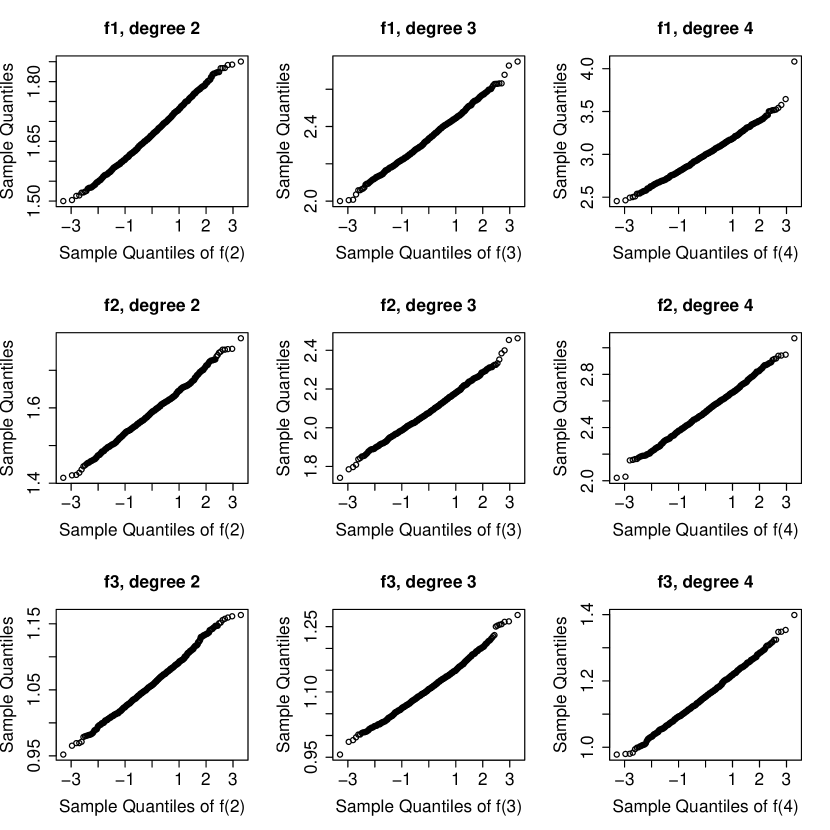
Figure 1: Boxplots of ee’s in different settings. The three rows correspond to the pa functions $f^{\scriptscriptstyle(1)}$, $f^{\scriptscriptstyle(2)}$, $f^{\scriptscriptstyle(3)}$, respectively and the three columns correspond to three network sizes, respectively. In each panel the horizontal axis is the degree and the vertical axis correspond to the value of the preference function and a boxplot of the 1,000 estimates. The ground truth is marked in red.

These plots suggest the following observations:

• The estimator is consistent, as our theorem shows. The quality improves when we have more nodes, hence more observations.

• For a fixed number of nodes, the quality of the estimator deteriorates fast when $k$ increases, exemplified by the substantial variability compared to the ground truth.

• Even if the ee has a large variance for large $k$’s, the sample median of $\hat{r}_{k}$ in each degree $k$ is still remarkably close to the truth.

• For a fixed number of nodes it appears that, when the ee makes larger errors, it is overestimating.

• The ee is not automatically monotone. However, we can slightly modify the estimator so that it is still consistent but always gives monotone results (cf. Chernozhukov et al. (2009)).

To summarize, the estimator performs as proven in our main result in Theorem 2, but the exact performance depends on the true pa function and the degrees of interest—if the true pa function increases slowly with respect to the degree, then it is easier to estimate the preference of low degrees, and harder to estimate the preference of high degrees and vice versa.

5.1 Sample variance study

We again run 1000 simulations of trees with pa functions of $f^{\scriptscriptstyle(1)}$, $f^{\scriptscriptstyle(2)}$, $f^{\scriptscriptstyle(3)}$, but now only simulate networks of size 1,000,000. We apply the ee to each simulated network and calculate the sample variance of the 1000 estimates for each given degree up to $70$, if the estimate is defined. The sample variances are plotted against the degrees in Figure 2. Denote the sample variance of the ee for degree $k$ by $s_{k}$. Inspection of these plots reveal the following:

• It appears that $\log s_{k}$ grows polynomially with respect to $\log k$. For the affine pa function $f^{\scriptscriptstyle(1)}$, it looks like $\log s_{k}$ is an affine function of $\log k$.

• The sample variance $s_{k}$ characterizes, to a certain extent, the difficulty of estimating $r_{k}$:

  • For small $k$’s, we see that $s^{\scriptscriptstyle(3)}_{k}<s^{\scriptscriptstyle(2)}_{k}<s^{\scriptscriptstyle(1)}_{k}$.

  • Then at about $k=17$, the blue line of $s^{\scriptscriptstyle(3)}_{k}$ first crosses the green line of $s^{\scriptscriptstyle(2)}_{k}$, i.e., $s^{\scriptscriptstyle(2)}_{k}<s^{\scriptscriptstyle(3)}_{k}<s^{\scriptscriptstyle(1)}_{k}$.

  • The blue line of $s^{\scriptscriptstyle(3)}_{k}$ crosses the red line of $s^{\scriptscriptstyle(1)}_{k}$ at around $k=18$. This means $s^{\scriptscriptstyle(2)}_{k}<s^{\scriptscriptstyle(1)}_{k}<s^{\scriptscriptstyle(3)}_{k}$.

  • The green line of $s^{\scriptscriptstyle(2)}_{k}$ crosses the red line of $s^{\scriptscriptstyle(1)}_{k}$ at approximately $k=35$, so from that point on $s^{\scriptscriptstyle(1)}_{k}<s^{\scriptscriptstyle(2)}_{k}<s^{\scriptscriptstyle(3)}_{k}$.

• On the one hand, for small $k$’s, the slower $f$ grows with $k$, the easier it is to estimate $r_{k}$. This is reflected in the observation that slower $f$ yield lower sample variance for small values of $k$. On the other hand, for large $k$’s, the faster $f$ grows with $k$, the easier it is to estimate $r_{k}$.

• The shapes of curves of $k\mapsto s_{k}$ for different $f$’s seems to indicate that the faster $f$ grows with $k$, the slower $\log s_{k}$ grows with $\log k$. The seemingly affine relations might be a consequence of the limiting power-law distribution, but it is unclear to us how these relate precisely.

The above observations seem intuitive because for $f$ that grows fast, there are more nodes of high degrees, and this can be expected to yield better results in estimating the preferences of higher degrees. However, as the total number of nodes is fixed, more nodes of high degrees mean fewer nodes of low degrees. This results in larger variances in estimating $r_{k}$ for small $k$’s.

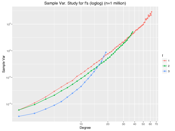
Figure 2: Sample Variance Study of EE. Different colors stand for different pa functions: the red corresponds to $f^{\scriptscriptstyle(1)}$, the green $f^{\scriptscriptstyle(2)}$ and the blue $f^{\scriptscriptstyle(3)}$. The scale on both axes are in $\log_{10}$. The three lines do not reach the same degrees as there are fewer nodes of high degrees when $f(k)$ grows slower in $k$.

5.2 Asymptotic normality of the estimator with the parametric rate?

We may wonder what is the asymptotic distribution of $\hat{r}_{k}(n)$ is, for any fixed $k$ and after proper rescaling, when $n\rightarrow\infty$. To answer this question, we discuss some simulation results here.

We fix the number of nodes to be 1,000,000 in all simulated networks for each pa function. Then we look at the ee’s in each simulation. For each $f$, we plot the qq-plot of each estimator for $k=2,3,4$ against the normal distribution. The results are summarized in Figure 3. Since the number of nodes is one million, we expect that the limiting distribution should have kicked in, assuming there is indeed a limiting distribution. The qq-plots indeed indicate that the ee’s have asymptotic normal distributions.

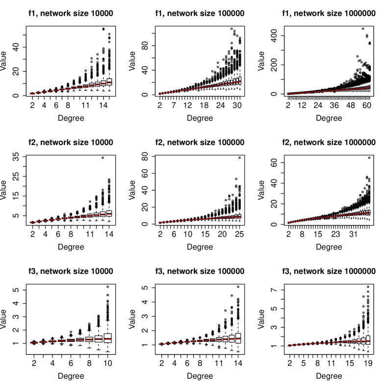
Figure 3: QQ-Plots of $\hat{r}_{2}(n)$, $\hat{r}_{3}(n)$ and $\hat{r}_{4}(n)$ with $n=10^{6}$ for $f^{\scriptscriptstyle(1)}$, $f^{\scriptscriptstyle(2)}$ and $f^{\scriptscriptstyle(3)}$ The rows correspond to the pa functions $f^{\scriptscriptstyle(1)}$, $f^{\scriptscriptstyle(2)}$ and $f^{\scriptscriptstyle(3)}$, respectively. The columns correspond to the degree $k=2,3,4$, on which we conduct our ee study, respectively.

We conjecture that, for fixed $k$,

$$\sqrt{n}(\hat{r}_{k}(n)-r_{k})\xrightarrow{d}N(0,\sigma_{k}^{2}),$$ (19)

where $\sigma_{k}^{2}$ only depend on $f$ and $k$ and $\xrightarrow{d}$ denotes convergence in distribution. To validate this conjecture, we perform the following simulation study. We fix the pa function to be $f^{\scriptscriptstyle(2)}$ and run 1,000 simulations for each of the three different network sizes 10,000, 100,000 and 1,000,000 and study the estimators of the preference on degree 2 only. If (19) is true, then the distribution of $\hat{r}_{2}(n)$ should stabilize after rescaling them with $\sqrt{n}$. We summarize the results in Figure 4.

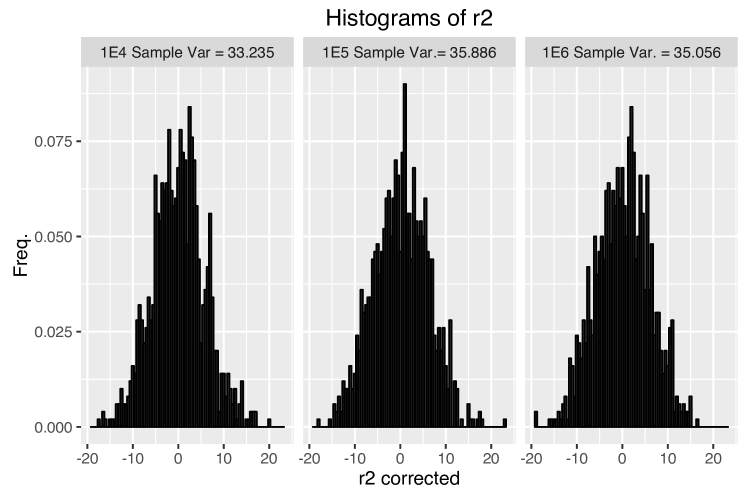
Figure 4: Histograms of $\sqrt{n}(\hat{r}_{2}(n)-r_{2})$ for $f^{\scriptscriptstyle(2)}$ with different network sizes The label r2 corrected on the $x$-axis indicates that the histograms show $\sqrt{n}(\hat{r}_{2}(n)-r_{2})$ (centered and rescaled with the parametric rate) instead of $\hat{r}_{2}(n)$. The sample variances of each simulation is on top of each subplot. The number of bins is 50.

The density estimations on the data of $\sqrt{n}(\hat{r}_{2}(n)-r_{2})$ for the three different values of $n$ are displayed in Figure 5. The fact that both the sample variances, histograms and density plots look rather stable after the $\sqrt{n}$-rescaling provides further evidence towards the conjecture in (19).

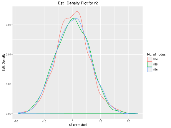
Figure 5: Estimated Density of $\sqrt{n}(\hat{r}_{2}(n)-r_{2})$ with different network sizes $n$

5.3 Discussion and open problems

In this paper, we have proposed an empirical estimator for the preferential attachment function in the setting of preferential attachment trees with (sub)linear preferential attachment functions. We rely on an embedding result that views the preferential attachment model as a continuous-time branching process observed at the moments where the branching process has a fixed size. We now discuss some open problems.

Beyond the tree setting.

It would be of interest to extend our analysis to settings where nodes enter the network with more than one edge. This corresponds to general preferential attachment graphs. In this case, the embedding results no longer hold, making the analysis substantially harder.

The limits of consistency.

Our main result in Theorem 2 shows that the ee is consistent for every ffixed $k$ fixed. For which $k=k_{n}\rightarrow\infty$ does consistency hold, and how does this depend on the pa function $f$? For which norms on $f$ does consistency hold?

Asymptotic normality.

Figures 3, 4 and 5 suggest asymptotic normality of the ee for fixed values of $k$ at the rate $\sqrt{n}$. How can such a statement be proved? It will also be interesting to study the convergence for increasing values of $k$. We expect the variance $\sigma_{k}^{2}$ in (19) to increase with $k$. This raises a problem of bias-variance trade-off when estimating the pa function for large degrees, much as in ordinary nonparametric estimation.

References

- Barabási and Albert [1999] A.-L. Barabási and R. Albert. Emergence of scaling in random networks. science, 286(5439):509–512, 1999.
- Barabási et al. [1999] A.-L. Barabási, R. Albert, and H. Jeong. Mean-field theory for scale-free random networks. Physica A: Statistical Mechanics and its Applications, 272(1):173–187, 1999.
- Barabási et al. [2000] A.-L. Barabási, R. Albert, and H. Jeong. Scale-free characteristics of random networks: the topology of the world-wide web. Physica A: Statistical Mechanics and its Applications, 281(1):69–77, 2000.
- Bollobás et al. [2001] B. Bollobás, O. Riordan, J. Spencer, G. Tusnády, et al. The degree sequence of a scale-free random graph process. Random Structures & Algorithms, 18(3):279–290, 2001.
- Bubeck et al. [2015] S. Bubeck, E. Mossel, and M. Z. Rácz. On the influence of the seed graph in the preferential attachment model. IEEE Transactions on Network Science and Engineering, 2(1):30–39, Jan 2015. ISSN 2327-4697. 10.1109/TNSE.2015.2397592.
- Chernozhukov et al. [2009] V. Chernozhukov, I. Fernández-val, and A. Galichon. Improving point and interval estimators of monotone functions by rearrangement. Biometrika, 96(3):559–575, 2009.
- Gao and van der Vaart [2017] F. Gao and A. van der Vaart. On the asymptotic normality of estimating the affine preferential attachment network models with random initial degrees. Stochastic Processes and their Applications, pages –, 2017. ISSN 0304-4149. https://doi.org/10.1016/j.spa.2017.03.008.
- Jagers [1975] P. Jagers. Branching processes with biological applications. Wiley, 1975.
- Krapivsky and Redner [2001] P. L. Krapivsky and S. Redner. Organization of growing random networks. Physical Review E, 63(6):066123, 2001.
- Móri [2002] T. Móri. On random trees. Studia Scientiarum Mathematicarum Hungarica, 39(1):143–155, 2002.
- Nerman [1981] O. Nerman. On the convergence of supercritical general (C-M-J) branching processes. Probability Theory and Related Fields, 57(3):365–395, 1981.
- Oliveira and Spencer [2005] R. Oliveira and J. Spencer. Connectivity transitions in networks with super-linear preferential attachment. Internet Mathematics, 2(2):121–163, 2005.
- Rudas et al. [2007] A. Rudas, B. Tóth, and B. Valkó. Random trees and general branching processes. Random Structures & Algorithms, 31(2):186–202, 2007.
- van der Hofstad [2017] R. van der Hofstad. Random graphs and complex networks, volume 1. Cambridge University Press, 2017.