On the use of kinetic energy preserving DG-schemes for large eddy simulation

Abstract

Recently, element based high order methods such as Discontinuous Galerkin (DG) methods and the closely related flux reconstruction (FR) schemes have become popular for compressible large eddy simulation (LES). Element based high order methods with Riemann solver based interface numerical flux functions offer an interesting dispersion dissipation behaviour for multi-scale problems: dispersion errors are very low for a broad range of scales, while dissipation errors are very low for well resolved scales and are very high for scales close to the Nyquist cutoff. In some sense, the inherent numerical dissipation caused by the interface Riemann solver acts as a filter of high frequency solution components. This observation motivates the trend that element based high order methods with Riemann solvers are used without an explicit LES model added. Only the high frequency type inherent dissipation caused by the Riemann solver at the element interfaces is used to account for the missing sub-grid scale dissipation. Due to under-resolution of vortical dominated structures typical for LES type setups, element based high order methods suffer from stability issues caused by aliasing errors of the non-linear flux terms. A very common strategy to fight these aliasing issues (and instabilities) is so-called polynomial de-aliasing, where interpolation is exchanged with projection based on an increased number of quadrature points. In this paper, we start with this common no-model or implicit LES (iLES) DG approach with polynomial de-aliasing and Riemann solver dissipation and review its capabilities and limitations. We find that the strategy gives excellent results, but only when the resolution is such, that about 40% of the dissipation is resolved. For more realistic, coarser resolutions used in classical LES e.g. of industrial applications, the iLES DG strategy becomes quite in-accurate. We show that there is no obvious fix to this strategy, as adding for instance a sub-grid-scale models on top doesn’t change much or in worst case decreases the fidelity even more. Finally, the core of this work is a novel LES strategy based on split form DG methods that are kinetic energy preserving. Such discretisations offer excellent stability with full control over the amount and shape of the added artificial dissipation. This premise is the main idea of the work and we will assess the LES capabilities of the novel split form DG approach. We will demonstrate that the novel DG LES strategy offers similar accuracy as the iLES methodology for well resolved cases, but strongly increases fidelity in case of more realistic coarse resolutions.

1 Introduction

Using high order Discontinuous Galerkin (DG) methods, and closely related methods such as flux reconstruction (FR) schemes, implicit large eddy simulation (iLES) approaches were recently applied to successfully simulate flows at moderate Reynolds numbers e.g. [39, 7, 3, 4, 14, 40, 31]. The approach used in these references does not add an explicit sub-grid scale model, such as e.g. eddy viscosity, but instead relies on the dissipation behaviour of the schemes due to Riemann solvers at element interfaces. High order discretisations, i.e. methods with polynomial degree $N\geq 3$, are usually used to obtain good dispersion behaviour which is necessary to accurately capture the interaction of different spatial scales. Within the references above, it is shown that for very high order polynomial degrees, the iLES DG discretisations are prone to aliasing issues due to the non-linearity of the flux functions. These aliasing issues can even cause instabilities and cause the simulation to crash. Within the references above, stabilisation in case of very high order polynomial degrees is done by applying so-called polynomial de-aliasing. There are several ways of implementing and interpreting polynomial de-aliasing. The goal however is always the same: account for the non-linearity of the flux function by either using a polynomial projection or by increasing the number of quadrature points for the approximation of the integrals. In [24], Kirby and Karniadakis demonstrated that cutting off $1/3$ of the highest modes in every time step for the incompressible Navier-Stokes equations (quadratic flux function) gives a stable approximation. They extended this for compressible flow, where they interpreted the non-linearity of the compressible Navier-Stokes fluxes as cubic and found that cutting off $1/2$ of the highest modes gives stability in all cases they tested. The non-linearity in the compressible case is however rational and thus there are also cases where this strategy fails, see e.g. [31, 19]. The issue of aliasing is mitigated somewhat by the use of Riemann solvers at element interfaces. For element based high order methods, the Riemann solver at the element interfaces provides numerical dissipation that acts in a high frequency filter-like way: it is almost zero for well resolved scales but gets very high for scales close to the Nyquist limit. This numerical dissipation behaviour paired with the good dispersion properties is the motivation to use element based high order methods such as the DG scheme with interface Riemann solvers for under-resolved turbulence simulations, often termed implicit LES (iLES), as no explicit sub-grid scale dissipation model is added.

In the following, we will use the iLES DG approach to simulate the decay of homogeneous isotropic turbulence (DHIT). The test case is a homogeneous isotropic turbulence freely decaying for about one large eddy turn over time ($T=\bar{v}(t_{start})/L_{int}\approx 1.3$). The Reynolds number based on the Taylor micro scale decays from $Re_{\lambda}\approx 162$ to $Re_{\lambda}\approx 97$. The LES initial state is obtained from a filtered DNS field. The DNS is simulated as in [41], with a pseudo-spectral code on $512^{3}$ DOF using the $2/3$ rule for de-aliasing. Similar test cases for LES were used for example in [22, 21, 14]. Figure 1 shows the resulting kinetic energy (KE) spectra for a relatively high resolved LES setting, $18$ cells per direction and polynomial degree $N=7$, i.e. $144$ DOF per direction in comparison with the DNS result. For the Riemann solver, we choose Roe’s approximate numerical flux function. We note that in this case polynomial de-aliasing is applied according to the $3/2$ rule (total of $12^{3}$ quadrature points per element), as the flow behaves almost incompressible, see e.g. [16].

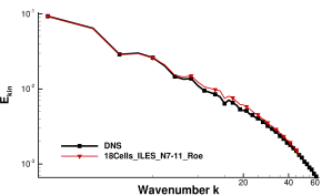
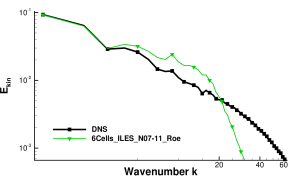
Figure 1: Decaying homogeneous isotropic turbulence DNS/LES kinetic energy spectra: a) iLES $144^{3}$ DOF b) iLES $48^{3}$ DOF. Both approximations use Roe’s approximate Riemann solver at the element interfaces.

With this particular iLES DG setup about $62.5\%$ of the total dissipation at $t_{0}$ can be resolved if we consider the theoretical Nyquist wavenumber $k_{Ny}=144/2=72$ for this discretisation with $144^{3}$ DOF. Assuming a more realistic (but still optimistic) approximation capability of the piece-wise polynomial ansatz space of $3$ points per wavenumber (PPW), then only about about $43.2\%$ of the KE dissipation is resolved. This setup is still somewhat well behaved: although under-resolved, the cut off wavenumber $k_{c}=144/3=48$ falls within the beginning of the dissipation range, which is the reason that the results obtained with the DG iLES approach are in excellent agreement with the reference direct numerical simulation (DNS).

However, in the available literature, simulations of the DHIT test case usually aim at considerable lower resolutions. In the spectral community $32^{3}$ points, e.g. [36], are commonly used for the assessments. Accounting for the difference between approximations with Fourier basis ($2$ PPW resolution limit) and polynomial basis (about $3$ PPW resolution limit), we increase the DG resolution to $48^{3}$ DOF, in particular we choose for the next setup $6^{3}$ elements with a polynomial degree of $N=7$. Using again the optimistic estimate of $3$ PPW the resulting cut-off wavenumber of this setup is $k_{c}=48/3=16$, which is comparable to the cut-off wavenumber of a spectral simulation with $32^{3}$ DOF, i.e. $k_{c}=32/2=16$. If we estimate the resolved total dissipation for this coarse setup, we only get about $0.9\%$ for the cut-off wavenumber $k_{c}=16$, which shows that this test case is severely under-resolved in comparison to the setup with $144^{3}$ DOF. Figure 1 shows that for such a resolution the DG iLES fails to match the reference DNS result. We observe a pile up of energy for mid range scales followed by a strong drop off of energy. Such a behaviour is indeed typical for upwind based iLES discretisations with very coarse resolutions, such as the present DG iLES configuration with Roe’s Riemann solver. A discussion on this typical behaviour of upwind schemes and a good overall review can be found in Drikakis [12].

As discussed, for the DG iLES approach the main dissipation is added by the Riemann solver at the element interfaces. Consequently, the amount and the ’shape’ of the numerical dissipation depends on the particular choice of the Riemann solver. Figure 2 shows results when comparing Roe’s approximate Riemann solver and the Lax-Friedrichs numerical flux. While there is a clear effect and influence by the choice of the interface numerical flux function, neither choice greatly improves the iLES result in comparison to the DNS reference, i.e. both suffer from the typical upwind behaviour mentioned above.

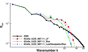
Figure 2: Decaying homogeneous isotropic turbulence DNS/LES kinetic energy spectra: iLES with different Riemann solvers. Red curve is the result with Lax-Friedrichs and green with Roe’s flux.

It is worth noting that the second ’parameter’ in the DG iLES approximation, the polynomial de-aliasing, cannot be omitted as the DG iLES without polynomial de-aliasing becomes unstable for this particular choice of polynomial degree (it might be stable for lower polynomial degrees, which results in higher artificial upwind dissipation). In conclusion, it seems that the DG iLES approach is very ’rigid’, rigid in the sense that there is not a lot of options to influence the dissipation behaviour of the scheme as polynomial de-aliasing is necessary and the only available parameter ’Which Riemann solver do we chose?’ doesn’t seem to provide means for substantially increasing the fidelity of the DG iLES. Adding explicit SGS dissipation to the described (iLES) schemes is difficult as usually the artificial dissipation interacts with the sub-grid scale model viscosity. It is then difficult to separate the effects, making turbulence modelling based on physical rationals very adventurous. This could be in fact the explanation, why the no-model or iLES DG approach is current state of the art in the DG community, as not really a clearly better strategy is known yet. Exemplary we show the effect of adding an explicit SGS model in Figure 3 for the standard Smagorinsky model, see A for details, and its high fidelity variant, the small-small variational multi scale model (VMS), see B for details.

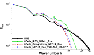
Figure 3: Decaying homogeneous isotropic turbulence DNS/LES kinetic energy spectra: polynomial de-aliasing, Roe’s Riemann solver and two different explicit sub grid scale eddy viscosity models

We find again that indeed there is no significant improvement of the result, independent of the SGS model constants used. This strongly hints towards a limiting applicability of upwind-type based iLES DG with de-aliasing for cases with relatively high resolution: Our numerical experiments show that roughly $40\%$ of the total dissipation should be resolved, which poses a natural plateau for this approach.Up to now, it seems that no remedy for this applicability plateau is available and known in literature. That is the reason why in this work we do not propose to modify or add models to the DG iLES to fix these issues, but propose a completely new approach instead!

We change the discretisation considerably and focus on an alternative approach for stabilising under-resolved DG discretisations, namely the strategy of using split forms for the non-linear terms [19], e.g. skew-symmetric splittings of the advective terms. The class of split form DG allows to inbuilt the de-aliasing in the discretisation of the volume terms. It is furthermore possible to construct a high order DG discretisation that is kinetic energy preserving, if an appropriate split form is chosen. Split forms are well known in the finite difference community [36, 37, 34, 29, 26, 10] and a multitude of variants exist. A good overview is given in Pirozzoli [37]. Priozzoli also presents a special variant of the splitting based on a three-way splitting of the non-linear flux terms, resulting in a kinetic energy preserving discretisation that is close to the scheme presented by Kennedy and Gruber [23]. Based on these split forms, it is possible to construct dissipation free DG schemes that still feature remarkable numerical robustness, sometimes even higher than the polynomial de-aliasing based approach [19]. This feature is exactly what we will exploit in this work: having a dissipation free base line scheme that is still robust offers the opportunity to add precisely the shape and amount of dissipation motivated by modelling sub-grid scale physics instead of e.g. Riemann solver dissipation that is constructed to capture shock physics.

Summarising, the goal in this work is to show how to construct dissipation free split form DG schemes with explicit sub-grid turbulence models and assess the performance of this novel strategy. We demonstrate that this strategy offers high potential for practical LES applications were only a small fraction of the total dissipation is resolved. We further demonstrate that it is possible to overcome the applicability plateau of the DG iLES approach and that with a dissipation free base line scheme we are able to add dissipation motivated by turbulence-physics.

The remainder of the article is organised as follows: In the next section, a small introduction to split form DG schemes is given. The next two chapters focus on numerical results for the DHIT with the conclusions and outlook given in the last section.

2 Numerical Methods

2.1 Discontinuous Galerkin Spectral Element Method

We consider the compressible Navier-Stokes equations (NSE) expressed in conservation form

$$\mathbf{U}_{t}+\mathbf{\nabla}_{x}\cdot\mathbf{F}(\mathbf{U},\mathbf{\nabla}_{x}\mathbf{U})=0,$$ (1)

where $\mathbf{U}$ denotes the vector of conserved quantities $\mathbf{U}=(\rho,\rho v_{1},\rho v_{2},\rho v_{3},\rho e)^{T}$, the subscript $t$ the time derivative and $\mathbf{\nabla}_{x}$ the gradient operator in physical space. The flux is the difference of advection and viscous fluxes, $\mathbf{F}=\mathbf{F}^{a}(\mathbf{U})-\mathbf{F}^{v}(\mathbf{U},\mathbf{\nabla}_{x}\mathbf{U})$, with the entries

$$\mathbf{F}^{a}_{l}(\mathbf{U})=\begin{pmatrix}\rho\,v_{l}\\ \rho\,v_{1}v_{l}+\delta_{1l}\,p\\ \rho\,v_{2}v_{l}+\delta_{2l}\,p\\ \rho\,v_{3}v_{l}+\delta_{3l}\,p\\ \rho\,ev_{l}+p\,v_{l}\end{pmatrix},\;\mathbf{F}^{v}_{l}(\mathbf{U},\mathbf{\nabla}_{x}\mathbf{U})=\begin{pmatrix}0\\ \tau_{1l}\\ \tau_{2l}\\ \tau_{3l}\\ \tau_{lj}v_{j}-q_{l}\end{pmatrix},$$ (2)

where $l=1,2,3$, denoting the Cartesian directions of the flux $\mathbf{F}_{1},\mathbf{F}_{2},\mathbf{F}_{3}$. We follow the usual nomenclature for $\rho,(v_{1},v_{2},v_{3})^{T},p,e$ denoting the density, velocity vector, pressure and specific total energy, respectively. The perfect gas law

$$p=\rho RT=(\kappa-1)\rho(e-\frac{1}{2}\mathbf{v}\cdot\mathbf{v}),\quad e=\frac{1}{2}\mathbf{v}\cdot\mathbf{v}+c_{v}T$$ (3)

is used to close the system of equations.

In this work we use a special DG variant, namely the discontinuous Galerkin spectral element collocation method (DGSEM) with Legendre Gauss-Lobatto (LGL) nodes. The LGL nodes are essential, as this choice guarantees the so-called summation-by-parts (SBP) property of the resulting DGSEM operator [15]. Up to now, split form DG is only available for this specific variant, as the SBP property is fundamental. The computational domain is subdivided into non-overlapping hexahedral elements which are transformed to reference space $\mathbf{\xi}$ via a transfinite mapping. Within the reference element, a tensor-product polynomial approximation is constructed: we use the tensor-product of the 1D LGL nodes and the associated tensor-product of 1D Lagrange polynomials, which gives $(N+1)^{3}$ DOF per element per unknown quantity for a given polynomial degree of $N$:

$$\mathbf{U}(\mathbf{\xi},t)\approx\sum\limits_{i,j,k=0}^{N}\mathbf{\hat{U}}_{ijk}(t)\psi_{ijk}(\mathbf{\xi})\,,\qquad\psi_{ijk}(\mathbf{\xi})=\ell_{i}(\xi^{1})\ell_{j}(\xi^{2})\ell_{k}(\xi^{3})\,,$$ (4)

with the 1D Lagrange basis functions defined as

$$\ell_{j}(\mathbf{\xi})=\prod_{i=0,i\neq j}^{N}\frac{\xi-\xi_{i}}{\xi_{j}-\xi_{i}},\quad j=0,...,N,$$ (5)

where $\{\xi_{i}\}_{i=0}^{N}$ are the LGL nodes. From this 1D Lagrange basis, we can directly compute the associated derivative matrix

$$D_{ij}=\ell_{j}^{\prime}(\mathbf{\xi}_{i}),\quad i,j=0,...,N,$$ (6)

store the LGL weights $\{\omega_{i}\}_{i=0}^{N}$ in the discrete mass-lumped diagonal mass matrix

$$M=diag([\omega_{0},...,\omega_{N}]),$$ (7)

and define the boundary matrix

$$B=diag([-1,0,...,0,1]).$$ (8)

These three 1D operator matrices are connected via the SBP property

$$(M\,D)+(M\,D)^{T}=B,$$ (9)

which guarantees consistency of discrete integration-by-parts based on the derivative matrix and the discrete inner product with LGL nodes.

For simplicity, we assume a Cartesian grid as used in our numerical tests for the DHIT test case. Details and the extension to general curvilinear elements are available in [19]. Furthermore, for the discretization of the second order viscous terms we resort to a standard method available in literature, namely, we use the approach introduced by Bassi and Rebay (BR) [1, 2] and analysed in Gassner et al. [18], where the gradient of the solution is introduced as an additional new unknown. With this, the second order problem is re-written into a larger system of first order partial differential equations. For the system of auxiliary gradients a standard DGSEM based on LGL is used, where the numerical flux at the element interfaces is chosen as the arithmetic mean. This DG gradient is then used to compute the viscous fluxes in the discrete Navier-Stokes equations. There are two different variants which can be used in the BR framework, namely BR1 (arithmetic mean of the viscous fluxes at the element interface) or BR2 (an additional artificial dissipation term depending on the interface jump of the solution). The BR2 scheme provides a mechanism to introduce additional numerical dissipation via the so-called penalty constant $\eta_{BR}\geq 1$: the larger this value, the higher the additional artificial interface dissipation.

The discretization of the advective Euler fluxes needs more care. Assuming Cartesian grids with size $\Delta x,\Delta y,\Delta z$ the transformation of the flux divergence in reference space is straight forward. For simplicity, we only focus on the term $\frac{1}{\Delta x}\mathbf{F}^{a}_{1}(\mathbf{U})_{\xi}$, i.e. the Cartesian flux in $\xi$-direction after transformation. The standard strong form LGL DGSEM for this term at an LGL node $(i,j,k)$ reads as

$$\frac{1}{\Delta x}\mathbf{F}^{a}_{1}(\mathbf{U})_{\xi}\big{|}_{ijk}\approx\frac{1}{M_{ii}}\left(\delta_{iN}\left[\mathbf{F}_{1}^{a,*}-\mathbf{F}_{1}^{a}\right]_{Njk}-\delta_{{i0}}\left[\mathbf{F}_{1}^{a,*}-\mathbf{F}^{a}_{1}\right]_{0jk}\right)+\sum_{m=0}^{N}D_{i\boldsymbol{m}}(\mathbf{F}^{a}_{1})_{\boldsymbol{m}jk},$$ (10)

where $\mathbf{F}_{1}^{a,*}$ is the numerical interface flux function, typically an approximate Riemann solver, and $(\mathbf{F}^{a}_{1})_{mjk}=\mathbf{F}^{a}_{1}(\boldsymbol{\hat{U}}_{ijk})$ is the non-linear Euler flux evaluated at the nodal solution value, i.e. the interpolation of the Euler flux at the LGL grid. The Kronecker delta $\delta_{ij}$ is equal to one when $i=j$ and zero otherwise and acts as a switch such that the boundary terms only affect the LGL boundary nodes.

As explained above, due to the non-linearity of the Euler fluxes, standard high order DG implementations such as the LGL DGSEM are prone to aliasing issues. An approach discussed above is to use polynomial de-aliasing, where the non-linear flux functions are projected onto the space of polynomials of degree $N$, instead of using an interpolation only. However, due to the rational non-linear nature of the Euler fluxes with respect to the conservative variables, it is not possible to implement an exact projection. Instead, this projection is constructed with an ’over-integration’ of the flux terms, i.e. by using a higher number of quadrature nodes. In our case we use the integer of $Q=3/2(N+1)-1$ as we assume weak compressibility effects due to the relatively low Mach number. A possible way of implementing this is via modal cut-off filters

$$\frac{1}{\Delta x}\mathbf{F}^{a}_{1}(\mathbf{U})_{\xi}\big{|}_{ijk}\approx P_{Q\to N}\frac{1}{M_{ii}}\left(\delta_{iQ}\left[\mathbf{F}_{1}^{a,*}-\mathbf{F}_{1}^{a}\right]_{Qjk}-\delta_{{i0}}\left[\mathbf{F}_{1}^{a,*}-\mathbf{F}^{a}_{1}\right]_{0jk}\right)+\sum_{m=0}^{Q}D_{i\boldsymbol{m}}(\mathbf{F}^{a}_{1})_{\boldsymbol{m}jk},$$ (11)

where the modal filter $P_{Q\to N}$ transforms the nodal space into modal space (tensor-product of orthogonal Legendre polynomials) deletes the modes from $N+1$ to $Q$ and transforms back to nodal space, see e.g. [14] for details.

The key of this work is an alternative technique for de-aliasing, namely the split form DG methodology. Split form DG is based on a remarkable property of diagonal norm SBP operators, discovered and introduced by Carpenter and Fisher, e.g. [13, 5]. They constructed so-called entropy stable forms of the volume terms by using

$$\frac{1}{\Delta x}\mathbf{F}^{a}_{1}(\mathbf{U})_{\xi}\big{|}_{ijk}\approx\frac{1}{M_{ii}}\left(\delta_{iN}\left[\mathbf{F}_{1}^{a,*}-\mathbf{F}_{1}^{a}\right]_{Njk}-\delta_{{i0}}\left[\mathbf{F}_{1}^{a,*}-\mathbf{F}^{a}_{1}\right]_{0jk}\right)+\sum_{m=0}^{N}2\,D_{i\boldsymbol{m}}\mathbf{F}^{a,\#}_{1}(\mathbf{U}_{ijk},\mathbf{U}_{\boldsymbol{m}jk}),$$ (12)

where they used a two-point entropy conserving numerical volume flux $\mathbf{F}^{a,\#}_{1}(\mathbf{U}_{ijk},\mathbf{U}_{\boldsymbol{m}jk})$. In Gassner et al. [19] it was shown that it is possible to choose every symmetric and consistent two-point numerical volume flux $\mathbf{F}^{a,\#}_{1}$ and that every choice results in a novel split form DGSEM. In particular, the authors identified specific choices of numerical volume fluxes to exactly reproduce well known split forms, such as the one of Pirozzoli [37]. This particular numerical volume flux is used in the present work and reads as

$$\mathbf{F}^{a,\#}_{1}(\mathbf{U}_{ijk},\mathbf{U}_{mjk})=\begin{bmatrix}\{\{\rho\}\}\{\{u\}\}\\ \{\{\rho\}\}\{\{u\}\}^{2}+\{\{p\}\}\\ \{\{\rho\}\}\{\{u\}\}\{\{v\}\}\\ \{\{\rho\}\}\{\{u\}\}\{\{w\}\}\\ \{\{\rho\}\}\{\{u\}\}\{\{h\}\}\end{bmatrix},$$ (13)

with

$$\{\{\alpha\}\}:=\frac{1}{2}\,(\alpha_{ijk}+\alpha_{mjk}).$$

In [19], it was also shown that the resulting split form DG scheme is kinetic energy preserving in the element and when choosing the element interface flux $\mathbf{F}_{1}^{a,*}$ equal to (13), the resulting split form DGSEM is kinetic energy preserving across the domain. Effectively, this means that the aliasing error in the kinetic energy preservation due to the discretisation of advective terms is eliminated. This split form kinetic energy preserving scheme is exactly our baseline scheme with zero artificial kinetic energy dissipation mentioned above. Starting with this dissipation free baseline method, it is possible to add Riemann solver type dissipation at the element interfaces by augmenting the central numerical flux $\mathbf{F}_{l}^{a,\#}$ at the interface with either Lax-Friedrichs type scalar dissipation or Roe type matrix dissipation to recover an unwinding type split form DG scheme. However, this baseline scheme offers many other ways of adding artificial dissipation, as we will discuss below in detail.

Finally, the semi discrete (split form) DGSEM is integrated in time with an explicit fourth order low storage Runge-Kutta method, [6]. The explicit time step is computed on the fly by a typical advective CFL condition.

3 Results for decaying isotropic turbulence

Figure 4 shows the no model result for the DHIT test case for a dissipation free scheme employing the flux splitting with the numerical flux of Pirozzoli (13) discussed above (labeled PI in the following figures).

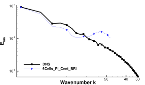
Figure 4: Decaying homogeneous isotropic turbulence DNS/LES kinetic energy spectra: no-model, central (“dissipation free“) numerical fluxes, BR1 scheme. Discretization with $6^{3}$ cells and $N=7$.

As seen in this plot the discrete solution describes approximately a $k^{2}$-slope close to the cut of wavenumber ($\approx 16$), known as equipartition spectrum. That is indeed an expected result and a direct consequence of the missing dissipation of the small scales. A result often observed when using no model pseudo spectral codes, eg. [36]. To the best of our knowledge that is the first time such a result is obtained with a DG scheme. It is furthermore remarkable that the dissipation free high order split form DGSEM with $6^{3}$ elements and $N=7$ is stable, although the simulation is severely under-resolved. Besides these two remarkable observations, it is also clear that this scheme does not provide an accurate approximation of the reference DNS result. However, as stated above, we will use this dissipation free scheme as a baseline scheme. The goal is to show that this scheme offers great potential when adding dissipation for sub-grid scale turbulence modelling. In fact, we will demonstrate several different strategies to include sub-grid scale dissipation.

Lastly, we note that in Figure 4 (and all other figures containing kinetic energy spectra for LES) the spectra of the LES is plotted up to the theoretical Nyquist frequency. The resolution limit of polynomials however is theoretically limited to $\pi$ PPW. For the dissipation free scheme in Figure 4 this limit corresponds well with the start where the kinetic energy decreases again ($48$ DOF $\widehat{=}$ $k_{\pi PPW}=15.28$, $144$ DOF $\widehat{=}$ $k_{\pi PPW}=45.84$). In the following sections, for our LES results this polynomial cut-off wavenumbers are the natural limits of our approximation. Our goal is therefor to obtain the best possible match with the DNS reference within this limit.

3.1 Split form DG iLES

Our first strategy is to use an iLES type strategy to account for the missing scales. We show, that the de-aliasing strategy (split form or polynomial de-aliasing) affects the behaviour of the iLES method, however the failure of iLES DG for coarse resolutions is not affected by the choice of de-aliasing strategy. We discuss in the following the deficiencies of the iLES DG approach and offer suggestions that the reason is missing dissipation for the large scales.

Starting with the baseline scheme that is dissipation free 4, we first add a classic Roe type matrix dissipation term at the element interfaces, which adds an upwind-type dissipation to the scheme based on linearised characteristics. This additional dissipation implicitly models the missing dissipation of the sub-grid scales, analogous to the standard DG iLES approach with polynomial de-aliasing discussed in the introduction. The core difference now is that we completely changed the de-aliasing mechanism and are thus able to investigate its effect on the iLES DG performance.

Figure 5 shows the result for the case where about $43.2\%$ of dissipation is resolved, i.e. the $144^{3}$ DOF setup.

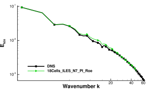
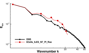
Figure 5: Decaying homogeneous isotropic turbulence DNS/LES kinetic energy spectra: a) Split form DG iLES $144^{3}$ DOF b) Split form DG iLES $48^{3}$ DOF. PI interface numerical flux is augmented with additional Roe type matrix dissipation.

Similar to the standard DG iLES results with polynomial de-aliasing, compare figure 1, the split form DG iLES produces excellent results for this setup. However, when decreasing again the resolution to a more realistic LES, where only $0.9\%$ of the total dissipation is resolved, the iLES DG approach fails again 5.

This is consistent with the DG iLES results obtained with polynomial de-aliasing as discussed in the introduction. We note again that in the iLES approach the dissipation stems solely from the element interface contributions. It was shown in [17, 32] that for high order DG schemes, this dissipation is focused on the highest wavenumbers. Consequently, this type of dissipation lacks a low wavenumber component, which provides a possible explanation for the failure: the theoretical findings of Kraichnan [25] state that for an infinite inertial KE range the resulting eddy viscosity is a constant (plateau) in the low wavenumbers and rising to a cusp towards the cut-off wavenumber. The plateau becomes especially relevant for coarse resolutions, or similarly for high Reynolds numbers, leading to a cut-off wavenumber in the inertial range. This is discussed in detail by Lesieur e.g. in [27].

The left part of Figure 6 shows the comparison of the coarse iLES with the two different de-aliasing strategies, namely the polynomial de-aliasing and the kinetic energy preserving split form. Both discretizations use the dissipation terms of Roe’s Riemann solver at the element interfaces. The almost identical KE spectra show clearly that in this case, the failure is due to the unsuited dissipation added by the Riemann solver, and not linked with the de-aliasing procedure. We note that a similar behaviour can be observed with Lax-Friedrichs type dissipation added at element interfaces.

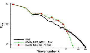
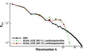
Figure 6: Decaying homogeneous isotropic turbulence DNS/LES with iLES results based on different de-aliasing strategies: red is based on the PI split form and green uses polynomial de-aliasing. Both setups use the dissipation term of Roe’s Riemann solver at the element interfaces.

Finally, we also plot the results obtained with the dissipation terms of the low dissipation Riemann solver of Oßwald et al. [35] in the right part of Figure 6. This variant is a modification to the original Roe solver to account for low Mach number flows (DHIT maximum local Mach number is about $0.1$, on average about $0.02$). This solver gives better results for DHIT when using finite volume schemes [35], compared to the classical Roe solver. The idea of the modification is to multiply the jump in the velocities at the interface by the local Mach number at the interface, resulting in a reduced dissipation in the momentum equations for low Mach number flows. We note that low dissipation Riemann solvers were also successfully used in a high order iLES DG approach with polynomial de-aliasing by [11], with an extension to a dynamic variational multi-scale model for the test case of plane channel flow in [33]. The authors clearly demonstrated the need for low dissipation Riemann solvers.

In contrast to the classic Roe dissipation results in the left part of Figure 6, in the right part of the Figure with the low dissipation Riemann solver of Oßwald et al. the two de-aliasing strategies behave differently. Indeed one can observe generally a slight improvement of the results for mid range scales, whereas the accuracy for higher wavenumbers is still quite low, underlining again the failure of the iLES approach for very coarse resolutions. It is worth pointing out that split form iLES DG variant is slightly more accurate for mid range scales compared to the polynomial de-aliasing approach and furthermore behaves somewhat similar to the no-dissipation case 4 for the small scales. This is due to the very low dissipation of the low Mach number modification in the momentum equations and thus due to a very low overall kinetic energy dissipation in combination with the kinetic energy preserving split form. We will demonstrate in section 5 that the split form result with the modified Roe Riemann solver can be drastically improved when an actual SGS turbulence model is added to account for the missing small scale dissipation in the momentum equations instead of using a Riemann solver type dissipation term in the momentum equations.

4 Split Form DG LES

Our second strategy is to use a purely explicit LES DG strategy based on the dissipation free split form result 4. Instead of adding numerical dissipation at the element interfaces via the Riemann solver, we show in this section the possibility of using explicit turbulence modelling for DHIT to account for the missing small scale dissipation. The results are remarkable, as we will show that by adding the simple Smagorinsky model already gives superior results compared to the iLES DG results discussed above. We note that for dissipation-free base discretisations, the standard Smagorinsky model can be expected to produce reasonably good results if the model constant is adjusted to the underlying discretisation scheme. Up to now, this strategy is only applicable for the novel dissipation free split form DG.

In the left part of Figure 7 the KE spectra is shown, adding only Smagorinsky’s model [38] to the dissipation free baseline scheme. The result is already acceptable, and for the first time a successful coarse resolution LES DG result is obtained.

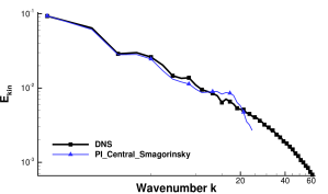
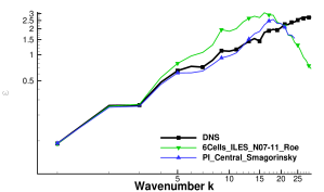
Figure 7: Left: Decaying HIT KE spectra for the dissipation free baseline scheme with explicit Smagorinsky model with constant $C_{s}=0.12$. Right: Comparison of dissipation rate spectra to the iLES DG approach with Roe type dissipation and polynomial de-aliasing.

We further plot in the right part of Figure 7 a comparison of the spectra of the dissipation rate $\epsilon$ to the iLES DG approach with classic Roe type dissipation and polynomial de-aliasing. It is remarkable that even with a rather simple and limited SGS model, the result of the explicit LES DG is clearly superior to the iLES DG result. The key to this result is a baseline scheme that is virtually dissipation free and at the same time robust for under-resolved simulations. Thus, the SGS model dissipation is not necessary to retain stability by adding dissipation to the dissipation free baseline scheme, but is used to account solely for missing small scale dissipation. This strict separation of stability and model dissipation also allows for a more precise analysis of the affect of the turbulence model: The spectra shows a slight energy underestimation of kinetic energy in the medium range wavenumbers. This is usually a secondary effect due to undamped small scale fluctuations. This modelling effect is well known and various examples can be found in literature, an overview is given again by e.g. Lesieur [27].

Nevertheless, the dissipation-free baseline scheme with explicit Smagorinsky model offers a superior result compared to the state of the art iLES DG strategy. It is thus reasonable to proceed and investigate more advanced turbulence models and assess if in contrast to the iLES approach advanced turbulence modelling within the split form DG approach actually improves the simulation.

5 Advanced Turbulence Modelling for Split Form DG LES

Our third strategy is to add a cusp like eddy viscosity mechanism to cure the secondary effect of undamped small scale fluctuations observed for the standard Smagorinsky approach observed in the previous section: In order to improve the method described in section 4 we show three possible ways of introducing additional damping for the small scales (cusp). The aim is to show that the dissipation free baseline scheme offers a lot of freedom and possibilities to design and control the overall amount and snape of the dissipation. All strategies are focused on improving the modelling of the missing small scale dissipation, as the aspect of robustness and numerical stability is already accounted for by using the dissipation free baseline split form DG scheme. The three strategies considered and tested are:

• adding a low dissipation Riemann solver [35] at the interface,

• adding a penalty in the viscous numerical flux (BR2 with $\eta_{BR}=2$),

• adding additional eddy-viscosity in a variational multi scale sense with a cusp profile over polynomial modes following Chollet et al. [9].

The first two methods implicitly add dissipation via the numerical interface fluxes in addition to the Smagorinsky model. In principal, these can be seen as a mixture of iLES and explicit LES. However, as pointed out above, the interface dissipation acts like a high frequency filter and affects the small scales while the influence on the rest of the scales is very small, i.e. it introduces an additional damping of the small scales only (cusp). We note that in DG it is possible to introduce numerical interface dissipation via the advective Riemann solver or the viscous numerical flux function. For the advective numerical dissipation, we chose the low dissipation Roe variant discussed above, as the classic Roe dissipation already destroys the accuracy as shown in previous sections. For the numerical dissipation of the viscous terms, we extend change the BR1 approach to the BR2 approach, where the an additional penalty term of the jump of the solution is added to the local gradients. The effect of this penalty can be adjusted by the BR2 constant $\eta_{BR}$. In contrast to the first two strategies, method iii) can be seen as a purely explicit LES with an advanced SGS model where dissipation is increased for the highest polynomial modes, which correspond to the small scale contents of the solution.

The results of the three advanced strategies are shown in Figure 8 and all three variants give an improved KE spectrum. The results of our investigations are that method iii) allows for the best fit with the DNS, if the model parameters are adjusted to the dissipation free split form DG baseline scheme. Details of this model are given in C.

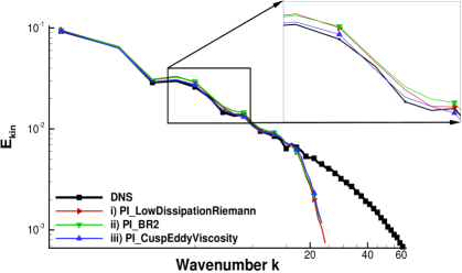
Figure 8: Decaying homogeneous isotropic turbulence DNS/LES with different modelling approaches. Results for modelling approaches almost collapse. Zoom in to region with largest differences.

Focusing on strategy i) with the low dissipation Roe Riemann solver, Figure 9 shows a comparison to the standard iLES DG approach with Roe dissipation and polynomial de-aliasing of the dissipation rate and the kinetic energy over time. The dissipation (kinetic energy) rate is computed in Fourier space as $\epsilon=2\nu\int_{k=1}^{16}k^{2}E(k)dk$ ($E_{Kin}=\int_{k=1}^{16}E(k)dk$) to obtain comparable results between LES and (filtered) DNS. We find that the standard iLES DG approach is not capable of reproducing the energy decay over time with this coarse resolution. In comparison, the novel method i) is in much better agreement with the (filtered) DNS result.

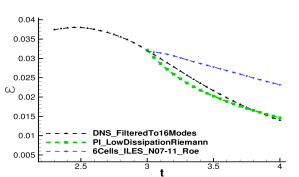
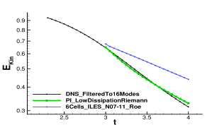
Figure 9: Comparison of dissipation rate (left) and kinetic energy (right) over time for (filtered DNS, split form LES DG, and standard iLES DG. Dissipation rate and kinetic energy are integrated in Fourier space up to $k=16$.

5.1 Pressure-dilatation fluctuations

An interesting side-effect of the advanced modelling results presented above is that it is now possible to observe other, formerly hidden, artefacts in the LES solution: pressure work can oscillate and strong fluctuations can be observed. It is important to note that by construction, neither the kinetic energy preserving PI split form nor the standard Smagorinsky model of the standard explicit LES DG approach presented above provide mechanisms to damp pressure of density fluctuations, especially regarding the inter element discontinuities of the DG approach. Thus, these quantities can and do oscillate as can be seen in the pressure work (syn. pressure-dilatation) $(\nabla\circ\mathbf{U})p$, Figure 10(a).

As investigated by [8], tailored Riemann solver dissipation, damping only density and pressure fluctuations, is sufficient to remove the oscillations. Among the three methods of section 5 only method i), the low dissipation Riemann solver, provides a mechanism to damp these fluctuations, compare Figure 10. The fluctuations in method ii) are somewhat smaller due to the added penalty terms in the computations of the gradients of the density and energy, Figure 10(c). Method iii) does not provide additional damping of pressure or density fluctuations by construction and thus the pressure work fluctuations in Figure 10(d) remain almost unchanged compared to 10(a).

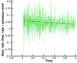
(a) Central+Smagorinsky (section 4)

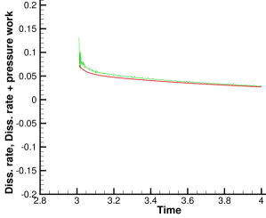
(b) Low dissipation Roe, method i) (section 5)

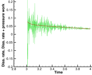
(c) BR2, method ii) (section 5)

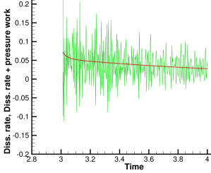
(d) Plateau-Cusp, method iii) (section 5)

Figure 10: Decaying homogeneous isotropic turbulence LES dissipation rate over time for different modelling approaches. Red: $\epsilon=2\nu\int_{\Omega}S_{ij}S_{ij}d\Omega$, green: $\epsilon+\int_{\Omega}(\nabla\circ\mathbf{U})pd\Omega$

In summary, the best LES results are obtained with method i): the baseline dissipation free split form DG scheme with a low dissipation Riemann solver that controls the fluctuations in density and pressure (but unaffected the dissipation in the momentum equations) with a standard Smagorinsky SGS model that provides suitable dissipation of the momentum equations and thus the kinetic energy. This clearly demonstrates the freedom in designing and precisely controlling the amount and shape of the added dissipation when the novel split form DG approach is used as a baseline scheme.

6 Discussion

6.1 Summary

This work presents the first extension of the novel split form DG framework [19] to explicit LES and iLES. We have first shown that there seems to be a common upper limit in the applicability of DG schemes for implicit LES. Only in cases where a substantial part of the dissipation is resolved by the DG approximation, the results are in good agreement with the reference. However, for realistic coarse resolutions, we show that the Riemann solver dissipation in combination with either de-aliasing strategy, polynomial de-aliasing or split forms, is not well suited as a sub-grid scale model for turbulence.

As a remedy, we propose a novel approach based on split forms that give non-linear robustness in combination with kinetic energy preservation, namely the split form introduced by Pirozzoli as a variant of the Kennedy and Gruber split form. This approach allows us to construct a baseline DG scheme with virtually no kinetic energy dissipation that is still stable for vortical dominated turbulence, even in case of severe under resolution. The main idea is that this stable but dissipation free DG scheme allows for precise control of the amount and shape of the dissipation added to model the effect of missing small scales, as no additional dissipation is needed to restore the robustness of the scheme in case of under resolution.

As a first result, this dissipation free baseline scheme in combination with a simple Smagorinsky model gives superior results compared to iLES DG. We further advance these results and introduce the following three strategies to add a cusp like behaviour to increase dissipation of the smallest scales:

• a kinetic energy consistent split-DG scheme,

• the low dissipation Roe-type Riemann solver of [35],

• and Smagorinsky’s SGS model.

All three advanced strategies yield improved results compared to the standard Smagorinsky model. But only method i) effectively controls oscillations in the pressure-dilatation and is thus the clear winner overall. It is also worth noting that method i) substantially improves the results in comparison to start of the art implicit LES DG. The results clearly underline the main idea that it is indeed possible to fully control and precisely adjust the dissipation in split form DG to account for missing small scales. As a final remark, the novel split form LES DG approach considerable reduces the computational cost by at least a factor of $3$ in our tests within our in-house DG simulation framework.

6.2 Outlook

The split form DG LES approach can be directly applied with more complex SGS models for more demanding applications. As a first result we show the computation of a plane turbulent channel flow employing the dynamic Smagorinsky model of Germano [20], with Lilly’s modification [28]. The flow is simulated for $Re_{\tau}=590$, with a $8^{3}$ grid and $N=7$ in a domain $[x,y,z]\in[0,2\pi]\times[-1,1]\times[0,\pi]$. Grid spacings are $\Delta x^{+}\approx 58$, $\Delta z^{+}\approx 29$ and $\Delta y^{+}_{min/max}\approx 7/28$, based on an equidistant inner cell point distribution. The result is compared to the DNS of [30] and the standard iLES DG approach with polynomial de-aliasing and Roe’s Riemann solver in Figure 11.

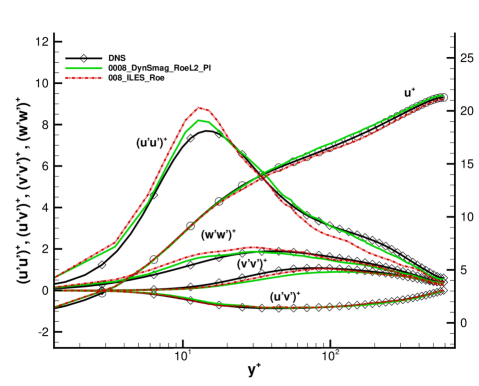
Figure 11: Plane turbulent channel flow, $Re_{\tau}=590$, $8$ cells per direction, $N=7$. Green line shows the novel split form DG LES approach with an explicit dynamic Smagorinsky model. Red curve shows standard implicit LES approach with polynomial de-aliasing and Roe’s Riemann solver. Reference DNS is taken from Moser [30], and no model LES

Both LES strategies yield acceptable results, even with this quite coarse resolution. However, the novel split form DG LES approach with explicit SGS turbulence modelling gives better Reynolds stress profiles, showing again excellent agreement with the DNS.

7 Acknowledgement

G.G has been supported by the European Research Council (ERC) under the European Union’s Eights Framework Program Horizon 2020 with the research project Extreme, ERC grant agreement no. 714487.

Appendix A Smagorinsky model

The classical Smagorinsky SGS stress, is defined as

$$\tau_{ij}=-2C_{S}^{2}\Delta^{2}|S(\nabla U)|(S_{ij}(\nabla U)-\frac{\delta_{ij}}{3}S_{ii}(\nabla U))$$ (14)

Where for the velocity gradients we use the lifted gradients. The filter width $\Delta$ is computed as the local cell volume divided be $(N+1)^{3}$. As usual $S$ is the strain rate tensor.

Appendix B High pass filtered Smagorinsky (VMS)

The high pass filtered Smagorinsky model (or variational multiscale Smagorinsky model, differing in the fiter operation only. We use a Galerkin projection as filter, i.e. a variational multi scale formulation) became popular recenlty, especially for wall bounded turbulence as the viscosity does not affect the large scales. The eddy viscosity is computed from the small scale gradients. We use a polynomial projection high-pass filter and apply it to the lifted gradients, denoting those as $\widetilde{\nabla U}$, cutting modes grater than $N_{filter}$. We compute the SGS stress as:

$$\tau_{ij}^{VMS}=-2C_{S}^{2}\Delta^{2}|S(\widetilde{\nabla U})|(S_{ij}(\widetilde{\nabla U})-\frac{\delta_{ij}}{3}S_{ii}(\widetilde{\nabla U}))$$ (15)

Appendix C Plataeu-Cusp model

In spectral methods it has proven advantageous to use an eddy viscosity with a plateau in the large scales and an a cusp towards the cut of wavenumber [9]. This is usually called the spectral eddy viscosity model (SPEVM). The shape is given in Fourier space by:

$$\nu^{t}(k|k_{c})=\nu^{t+}(k|k_{c})\left(\frac{E(k_{c},t)}{k_{c}}\right)^{(1/2)}$$ (16)

$$\nu^{t+}(k|k_{c})=0.267(1+34.5e^{-3.03(k_{c}/k)})$$ (17)

We seek to add a similar cusp in modal polynomial space. We reformulate the viscosity distribution as:

$$\nu^{t+}(N+1|N_{c}+1)=9.21e^{-3.03((N_{c}+1)/(N+1))})$$ (18)

This distribution we use as input to a polynomial projection high-pass filter and apply it to the lifted gradients, denoting those as $\widetilde{\nabla U}$. We compute the SGS stress in analogy to the high pass filtered eddy viscosity models (or VMS) as:

$$\tau_{ij}^{cusp}=-2C_{cusp}\Delta^{2}|S(\widetilde{\nabla U})|(S_{ij}(\widetilde{\nabla U})-\frac{\delta_{ij}}{3}S_{ii}(\widetilde{\nabla U}))$$ (19)

This ”cusp” stress we add to the classical Smagorinsky SGS stress, defined equivalent without high-pass filtered gradients

$$\tau_{ij}=-2C_{S}\Delta^{2}|S(\nabla U)|(S_{ij}(\nabla U)-\frac{\delta_{ij}}{3}S_{ii}(\nabla U))$$ (20)

For the result above we chose $C_{Cusp}=0.33^{2}$ and $C_{S}=0.13^{2}$.

Appendix D Dynamic Smagorinsky

The SGS stress of the classical Smagorinsky model is defined as

$$\tau_{ij}=-2C_{S}\Delta^{2}|S(\nabla U)|(S_{ij}(\nabla U)-\frac{\delta_{ij}}{3}S_{ii}(\nabla U)).$$ (21)

The dynamic procedure determines the constant $C_{S}$ depending on the flow:

$$C_{S}\Delta^{2}=-\frac{1}{2}\frac{<L_{ij}M_{ij}>}{<M_{ij}M_{ij}>}$$ (22)

with $<>$ an average operator over homogeneous directions. We chose to average over Y-Planes within a DG cell. The Germano identity is defined as

$$L{ij}=\widetilde{u_{i}u_{j}}-\widetilde{u_{i}}\widetilde{u_{j}}$$ (23)

with $\tilde{.}$ denoting a Galerkin projection filter operation, applied in x-z planes. We chose the test filter to $N_{testfilter}=3$, while the computational polynomial degree was $N=7$. That results to a filter width ratio of $(N)/(N_{testfilter})\approx 2.3$.
Also

$$M_{ij}=\widetilde{|S|(S_{ij}(\nabla U)-\frac{\delta_{ij}}{3}S_{ii}(\nabla U))}-\frac{\widetilde{\Delta}}{\Delta}|S(\widetilde{\nabla U})|(S_{ij}(\widetilde{\nabla U})-\frac{\delta_{ij}}{3}S_{ii}(\widetilde{\nabla U}))$$ (24)

Appendix E Channel flow details

For brevity we omitted details of the channel flow setup above. In this appendix we complement this. For the channel flow the second method of Bassi and Rebay (BR2) [2] was used. The penalty constant $\eta_{BR2}$ is chosen to $1$ at all inner (i.e. not wall boundaries) cell interfaces. In contrast to the first method of Bassi and Rebay (BR1), used for the DHIT simulations, the BR2 scheme is not artificial dissipation free. By choosing $\eta_{BR2}=1$ the methods are similar in that respect, as the lifting numerical flux becomes central, with the difference that for BR2 the surface gradients are only penalized according to the local jump of the solution at the respective interface. Using BR2 rises the possibility to add an additional penalty to the gradients at wall boundaries. With the given coarse resolution the velocities at the wall would otherwise be unacceptable large. This is a result of the weak wall boundaries commonly used for DG schemes. We set $\eta_{BR2}=40$ in order to obtain small velocities at the wall.
A constant pressure source term $dp/dx$ is used to force the flow, which prescribes the Reynolds number of the flow exactly. The simulations are run until the bulk velocity statistically converged. Quantities plotted in 11 are obtained by averaging over homogeneous directions.
The grid cells size is constant in x and z direction, in y direction a bell shape stretching is used with a ratio of $4$ from largest to smallest grid cell. In all directions $8$ cells are used.

References

- [1] Bassi, F., and Rebay, S. A high order accurate discontinuous finite element method for the numerical solution of the compressible Navier–Stokes equations. Journal of Computational Physics 131 (1997), 267–279.
- [2] Bassi, F., Rebay, S., Mariotti, G., Pedinotti, S., and Savini, M. A high-order accurate discontinuous finite element method for inviscid an viscous turbomachinery flows. In Proceedings of 2nd European Conference on Turbomachinery, Fluid and Thermodynamics (Technologisch Instituut, Antwerpen, Belgium, 1997), R. Decuypere and G. Dibelius, Eds., pp. 99–108.
- [3] Beck, A., Flad, D., Tonhäuser, C., and Munz, C.-D. On the influence of polynomial de-aliasing on subgrid scale models. Flow, Turbulence and Combustion under revision (2015).
- [4] Beck, A. D., Bolemann, T., Flad, D., Frank, H., Gassner, G. J., Hindenlang, F., and Munz, C.-D. High-order discontinuous Galerkin spectral element methods for transitional and turbulent flow simulations. International Journal for Numerical Methods in Fluids 76, 8 (2014), 522–548.
- [5] Carpenter, M. H., Fisher, T. C., Nielsen, E. J., and Frankel, S. H. Entropy stable spectral collocation schemes for the navier–stokes equations: Discontinuous interfaces. SIAM Journal on Scientific Computing 36, 5 (2014), B835–B867.
- [6] Carpenter MH, Kennedy CA, B. H. V. S. V. V. Fourth-order runge-kutta schemes for fluid mechanics applications. JOURNAL OF SCIENTIFIC COMPUTING 25, 1 (October 2005), 157–194.
- [7] Carton de Wiart, C., and Hillewaert, K. DNS and ILES of transitional flows around a SD7003 using a high order discontinuous Galerkin method. In Seventh International Conference on Computational Fluid Dynamics (ICCFD7) (2012).
- [8] Chandrashekar, P. Kinetic energy preserving and entropy stable finite volume schemes for compressible euler and navier-stokes equations. arXiv preprint arXiv:1209.4994 (2012).
- [9] Chollet, J. Two-point closure used for a sub-grid scale model in large eddy simulations. In Turbulent Shear Flows 4. Springer, 1985, pp. 62–72.
- [10] Desjardins, O., Blanquart, G., Balarac, G., and Pitsch, H. High order conservative finite difference scheme for variable density low mach number turbulent flows. Journal of Computational Physics 227, 15 (2008), 7125–7159.
- [11] Diosady, L., and Murman, S. Higher-order methods for compressible turbulent flows using entropy variables. AIAA Paper 294 (2015).
- [12] Drikakis, D., Hahn, M., Mosedale, A., and Thornber, B. Large eddy simulation using high-resolution and high-order methods. Philosophical Transactions of the Royal Society of London A: Mathematical, Physical and Engineering Sciences 367, 1899 (2009), 2985–2997.
- [13] Fisher, T. C., and Carpenter, M. H. High-order entropy stable finite difference schemes for nonlinear conservation laws: Finite domains. Journal of Computational Physics 252 (2013), 518–557.
- [14] Flad, D., Beck, A., and Munz, C.-D. Simulation of underresolved turbulent flows by adaptive filtering using the high order discontinuous galerkin spectral element method. Journal of Computational Physics 313 (2016), 1–12.
- [15] Gassner, G. A skew-symmetric discontinuous Galerkin spectral element discretization and its relation to SBP-SAT finite difference methods. SIAM Journal on Scientific Computing 35, 3 (2013), A1233–A1253.
- [16] Gassner, G., and Beck, A. On the accuracy of high-order discretizations for underresolved turbulence simulations. Theoretical and Computational Fluid Dynamics 27, 3-4 (2013), 221–237.
- [17] Gassner, G., and Kopriva, D. A comparison of the dispersion and dissipation errors of Gauss and Gauss-Lobatto discontinuous Galerkin spectral element methods. SIAM J. Scientific Computing 33, 5 (2011), 2560–2579.
- [18] Gassner, G., Winters, A., Hindenlang, F., and Kopriva, D. The br1 scheme is stable for the compressible navier-stokes equations. submitted to Journal of Scientific Computing.
- [19] Gassner, G. J., Winters, A. R., and Kopriva, D. A. Split form nodal discontinuous galerkin schemes with summation-by-parts property for the compressible euler equations. arXiv preprint arXiv:1604.06618 (2016).
- [20] Germano, M., Piomelli, U., Moin, P., and Cabot, W. H. A dynamic subgrid-scale eddy viscosity model. Physics of Fluids A: Fluid Dynamics (1989-1993) 3, 7 (1991), 1760–1765.
- [21] Hickel, S., Adams, N. A., and Domaradzki, J. A. An adaptive local deconvolution method for implicit les. Journal of Computational Physics 213, 1 (2006), 413–436.
- [22] Hughes, T. J., Mazzei, L., and Jansen, K. Large eddy simulation and the variational multiscale method. Computing and Visualization in Science 3, 1-2 (2000), 47–59.
- [23] Kennedy, C., and Gruber, A. Reduced aliasing formulations of the convective terms within the Navier–Stokes equations for a compressible fluid. Journal of Computational Physics 227 (2008), 1676–1700.
- [24] Kirby, R., and Karniadakis, G. De-aliasing on non-uniform grids: algorithms and applications. Journal of Computational Physics 191 (2003), 249–264.
- [25] Kraichnan, R. H. Eddy viscosity in two and three dimensions. Journal of the Atmospheric Sciences 33, 8 (1976), 1521–1536.
- [26] Kravchenko, A., and Moin, P. On the effect of numerical errors in large eddy simulations of turbulent flows. Journal of Computational Physics 131, 2 (1997), 310–322.
- [27] Lesieur, M., and Metais, O. New trends in large-eddy simulations of turbulence. Annual review of fluid mechanics 28, 1 (1996), 45–82.
- [28] Lilly, D. K. A proposed modification of the germano subgrid-scale closure method. Physics of Fluids A: Fluid Dynamics (1989-1993) 4, 3 (1992), 633–635.
- [29] Mittal, R., and Moin, P. Suitability of upwind-biased finite difference schemes for large-eddy simulation of turbulent flows. AIAA journal 35, 8 (1997), 1415–1417.
- [30] Moser, R. D., Kim, J., and Mansour, N. N. Direct numerical simulation of turbulent channel flow up to re= 590. Phys. Fluids 11, 4 (1999), 943–945.
- [31] Moura, R., Mengaldo, G., Peiró, J., and Sherwin, S. On the eddy-resolving capability of high-order discontinuous galerkin approaches to implicit les/under-resolved dns of euler turbulence. Journal of Computational Physics (2016).
- [32] Moura, R., Sherwin, S., and Peiró, J. Linear dispersion–diffusion analysis and its application to under-resolved turbulence simulations using discontinuous galerkin spectral/hp methods. Journal of Computational Physics 298 (2015), 695–710.
- [33] Murman, S. M., Diosady, L. T., Garai, A., and Ceze, M. A space-time discontinuous-galerkin approach for separated flows. Work 10 (2016), 5.
- [34] Nagarajan, S., Lele, S. K., and Ferziger, J. H. A robust high-order compact method for large eddy simulation. Journal of Computational Physics 191, 2 (2003), 392–419.
- [35] Oßwald, K., Siegmund, A., Birken, P., Hannemann, V., and Meister, A. L2roe: a low dissipation version of roe’s approximate riemann solver for low mach numbers. International Journal for Numerical Methods in Fluids (2015).
- [36] Park, N., Yoo, J. Y., and Choi, H. Discretization errors in large eddy simulation: on the suitability of centered and upwind-biased compact difference schemes. Journal of Computational Physics 198, 2 (2004), 580–616.
- [37] Pirozzoli, S. Numerical methods for high-speed flows. Annual review of fluid mechanics 43 (2011), 163–194.
- [38] Smagorinsky, J. General circulation experiments with the primitive equations. Mon. Wea. Rev. 91 (1963), 99–164.
- [39] Uranga, A., Persson, P.-O., Drela, M., and Peraire, J. Implicit large eddy simulation of transition to turbulence at low Reynolds numbers using a discontinuous Galerkin method. International Journal for Numerical Methods in Engineering 87, 1-5 (2011), 232–261.
- [40] Wiart, C. C., Hillewaert, K., Bricteux, L., and Winckelmans, G. Implicit les of free and wall-bounded turbulent flows based on the discontinuous galerkin/symmetric interior penalty method. International Journal for Numerical Methods in Fluids 78, 6 (2015), 335–354.
- [41] Yamazaki, Y., Ishihara, T., and Kaneda, Y. Effects of wavenumber truncation on high-resolution direct numerical simulation of turbulence. Journal of the Physical Society of Japan 71, 3 (2002), 777–781.