Optimizing the energy with quantum Monte Carlo: A lower numerical scaling for Jastrow-Slater expansions

Abstract

We present an improved formalism for quantum Monte Carlo calculations of energy derivatives and properties (e.g. the interatomic forces), with a multideterminant Jastrow-Slater function. As a function of the number $N_{e}$ of Slater determinants, the numerical scaling of $O(N_{e})$ per derivative we have recently reported is here lowered to $O(N_{e})$ for the entire set of derivatives. As a function of the number of electrons $N$, the scaling to optimize the wave function and the geometry of a molecular system is lowered to $O(N^{3})+O(NN_{e})$, the same as computing the energy alone in the sampling process. The scaling is demonstrated on linear polyenes up to C₆₀H₆₂ and the efficiency of the method is illustrated with the structural optimization of butadiene and octatetraene with Jastrow-Slater wave functions comprising as many as 200000 determinants and 60000 parameters.

I Introduction

Quantum Monte Carlo methods (QMC) are first-principle methods which can efficiently solve the Schrödinger equation. For fermionic systems, they are powerful variational approaches because they can handle a large variety of variational wave functions $\Psi({\bf R})$, where ${\bf R}=({\bf r}_{1}\dots\bf r_{N})$ represents the coordinates of the $N$ electrons of the system. Here, the vector ${\bf r}_{i}=(x_{i},y_{i},z_{i},\sigma_{i})$ indicates the 3 spatial coordinates of the electron $i$, $(x_{i},y_{i},z_{i})$ and its spin component $\sigma_{i}$ ($\sigma_{i}=\pm\frac{1}{2}$). This flexibility stems from the fact that integrals are not computed analytically but from a stochastic sampling. For example, the variational energy is

$$E={\int d{\bf R}\Psi^{2}({\bf R})\frac{\hat{H}\Psi}{\Psi}({\bf R})}\,$$ (1)

where $\hat{H}$ is the Hamiltonian and $\Psi$ is normalized, and can be interpreted as the expectation value of a random variable, the so-called local energy $E_{L}={\hat{H}\Psi}/{\Psi}$ on the probability density $\Psi^{2}({\bf R})$. QMC methods can be used as benchmark methods also for relatively large systems thanks to their favorable scaling with the number of particles $N$. For a given parametrization of $\Psi$, $E$ is typically computed with a scaling $O(N^{2})$ in memory requirements and $O(N^{3})$ in CPU per Monte Carlo step. In practice, one needs to optimize the parameters of $\Psi$ and the geometry of a molecular system. Despite the availability of stable wave function optimization methods Umrigar et al. (2007), such techniques remain costly and one of the main reasons is that a large number of derivatives of $E$ (typically $O(N^{2})$) has to be computed. Lowering the numerical scaling per derivative is therefore important. For single determinants, Sorella et al. have found that the low-variance estimators of the $3N_{\rm atoms}=O(N)$ intermolecular forces can be calculated with a scaling $O(N^{3})$ instead of $O(N^{4})$ with the use of algorithmic differentiation techniques Sorella and Capriotti (2010). We have recently recovered the same reduction using transparent matricial formulas and extended it to the $O(N^{2})$ orbital coefficients Filippi, Assaraf, and Moroni (2016). For expansions over additional $N_{e}$ Slater determinants, $D_{i}$, multiplied by a positive Jastrow correlation factor $J({\bf R})$,

$$\Psi({\bf R})=J({\bf R})\Phi({\bf R})=J({\bf R})\sum_{i=0}^{N_{e}}c_{i}D_{i}\,,$$ (2)

Clark et al. have proposed a method to compute $\Psi$ with a scaling $O(N_{e})$ and $E_{L}$ with a scaling $O(NN_{e})$ Clark et al. (2011) that we have further reduced to $O(N_{e})$ and extended to any derivative of $E_{L}$ Filippi, Assaraf, and Moroni (2016). The derivatives of $E_{L}$ are useful because they are involved in low-variance estimators for forces and observables Assaraf and Caffarel (1999); Filippi and Umrigar (2000); Assaraf and Caffarel (2003). At the origin of this reduction is the observation that the local energy can be written in terms of a first-order (logarithmic) derivative of the determinantal component, $\partial_{\lambda}\Phi/\Phi$.

In this paper, we show that the scaling $O(N_{e})$ per derivative can be further improved to $O(N_{e})$ for any set of derivatives of $\Psi$ and $E_{L}$. The core observation is that the determinantal part $\Phi$ is a function of the matrix elements $\tilde{A}_{ij}=\phi_{j}({\bf r}_{i})$ where $\phi_{j}$ is an orbital and $i$ an electron index, and that any derivative of $\Phi$ can be computed using a simple trace formula involving the matrix $\Gamma$ defined as the logarithmic gradient of $\Phi$ with respect to $\tilde{A}$. The first derivatives of the local energy $\partial_{\mu}E_{L}$ can then be expressed as traces involving $\Gamma$ and one of its derivative $\partial_{\lambda}\Gamma$: many derivatives of $\Psi$ and $E_{L}$ are obtained efficiently because the matrices $\Gamma$ and $\partial_{\lambda}\Gamma$ are computed only once for the whole set of parameters $\{\mu\}$. Consequently, the calculation of all derivatives of $E$ with respect to all parameters of the wave function (Jastrow parameters, orbital coefficients, the coefficients of the expansion $\{c_{i}\}$, and all nuclear positions) has now the same scaling as the calculation of $E$ alone, opening the path to full optimization of large multideterminant expansions.

In the next Section, we outline the main idea and introduce the matrix $\Gamma$. In Section III, we present a formula to compute $\Gamma$ at a cost $O(N^{3})+O(N_{e})$ and, in Section IV, discuss the formulas for the second derivative of $\Phi$ and, specifically, the first derivatives of $E_{L}$. In Section V, we demonstrate the scaling of the computation of interatomic forces with multideterminant wave functions on polyenes up to C₆₀H₆₂ and, in the last Section, apply the scheme to the optimization of multideterminant wave functions and geometries of butadiene and octatetraene.

II Derivative of the determinantal expansion

The determinantal component $\Phi$ in the Jastrow-Slater expansion of Eq. (2) is a linear combination of $N_{e}+1$ Slater determinants

$$\Phi=\sum_{I=0}^{N_{e}}c_{I}\text{det}({A}_{I})\,.$$ (3)

For a system including $N$ electrons, the matrix $A_{I}$ is an $N\times N$ Slater matrix, built from $N$ of the $N_{\rm orb}$ molecular spin-orbitals $\phi_{i}({\bf r})$ $(1\leq i\leq N_{\rm orb})$. Mathematically, $A_{I}$ comprises $N$ columns of the $N\times N_{\rm orb}$ matrix $\tilde{A}$ defined as follows

$$\tilde{A}_{ij}=\phi_{j}({\bf r}_{i})\,.$$ (4)

In general, one needs to compute many derivatives of $\Phi$ with respect to different parameters of $\tilde{A}$. These parameters can be the electron coordinates, nuclei coordinates, orbital coefficients, basis-function parameters and so on. The derivative of $\Phi$ with respect to a given parameter $\mu$ in $\tilde{A}$ is obtained from the chain rule

$$\partial_{\mu}\ln(\Phi)=\frac{\partial\ln(\Phi)}{\partial\tilde{A}_{ij}}\partial_{\mu}{\tilde{A}}_{ij}=\text{tr}(\Gamma\partial_{\mu}\tilde{A})\,,$$ (5)

where a summation on repeated indices is implied and we have introduced $\Gamma$, that is, the gradient of $\ln(\Phi)$ with respect to the matrix elements of $\tilde{A}$

$$\Gamma_{ji}=\frac{\partial\ln\Phi}{\partial\tilde{A}_{ij}}\,.$$ (6)

The trace formula (5) is at the core of greater efficiency in computing many derivatives of $\Phi$ because the $N\times N_{\rm orb}$ matrix $\Gamma$ depends only on $\tilde{A}$ and not on $\partial_{\mu}\tilde{A}$. For a given configuration ${\bf R}$ in the Monte Carlo sample, $\Gamma$ is computed only once for all the set of derivatives. In addition, $\Gamma$ can be evaluated efficiently, at a cost $O(N^{3})+O(N_{e})$ as we will see in the next Section. Once $\Gamma$ is computed and stored, any new derivative $\partial_{\mu}\ln(\Phi)$ requires to calculate besides $\partial_{\mu}\tilde{A}$ the trace (5) at a cost $O(N_{\rm orb}\times N)$. What is important here is that this scaling is independent on $N_{e}$ and leads to vast improvements over previous methods Filippi, Assaraf, and Moroni (2016); Clark et al. (2011) when $N_{e}$ and the number of derivatives are large.

Finally, also quantities like the local energy or the value of the wave function after one electron move, can be computed using this trace formula (5). This is because one-body operators can be also expressed as first order derivatives of $\ln\Phi$ when applied to a Jastrow-Slater expansion Filippi, Assaraf, and Moroni (2016).

III Efficient evaluation of the matrix $\Gamma$

III.1 Convenient expression for $\Phi$

The determinants of the Slater matrices $A_{I}$ can be computed efficiently because $A_{I}$ usually differs by a few columns from a reference Slater matrix $A$. For example, let $A$ be the $4\times 4$ Slater matrix built with the orbitals $\phi_{1},\phi_{2},\phi_{3},\phi_{4}$:

$$A = \left(\begin{array}[]{ccccc}\tilde{A}_{1}&\tilde{A}_{2}&\tilde{A}_{3}&\tilde{A}_{4}\end{array}\right)\,,$$ (8)

where the notation $\tilde{A}_{i}$ stands for the $i^{th}$ column of $\tilde{A}$. The Slater matrix of a double excitation $(3,4)\to(5,7)$ is

$$A_{I} = \left(\begin{array}[]{ccccc}\tilde{A}_{1}&\tilde{A}_{2}&\tilde{A}_{5}&\tilde{A}_{7}\end{array}\right)\,.$$ (10)

Here, $A_{I}$ and $A$ differ only in the 2 last columns. The determinant of $A_{I}$ is

$$\text{det}(A_{I})=\text{det}(A)\text{det}(A^{-1}A_{I})$$

and

$$A^{-1}A_{I} = \left(\begin{array}[]{ccccc}A^{-1}\tilde{A}_{1}&A^{-1}\tilde{A}_{2}&A^{-1}\tilde{A_{5}}&\tilde{A}^{-1}\tilde{A}_{7}\end{array}\right)=\left(\begin{array}[]{cccc}1&0&(A^{-1}\tilde{A})_{15}&(A^{-1}\tilde{A})_{17}\\ 0&1&(A^{-1}\tilde{A})_{25}&(A^{-1}\tilde{A})_{27}\\ 0&0&(A^{-1}\tilde{A})_{35}&(A^{-1}\tilde{A})_{37}\\ 0&0&(A^{-1}\tilde{A})_{45}&(A^{-1}\tilde{A})_{47}\\ \end{array}\right)\,,$$ (16)

where a column of the identity matrix arises whenever $A_{I}$ and $A$ share the same column. The determinant of $A^{-1}A_{I}$ is readily evaluated:

$$\text{det}(A^{-1}A_{I})=\text{det}\left(\begin{array}[]{cc}(A^{-1}\tilde{A})_{35}&(A^{-1}\tilde{A})_{37}\\ (A^{-1}\tilde{A})_{45}&(A^{-1}\tilde{A})_{47}\\ \end{array}\right)\,.$$ (17)

More generally, the determinant of $A^{-1}A_{I}$ for a $k_{I}^{th}$-order excitation is the determinant of a $k_{I}\times k_{I}$ submatrix. Such a submatrix can always be written as follows

$$\alpha_{I}=P_{I}^{T}A^{-1}\tilde{A}Q_{I}\,,$$ (18)

where, in our example,

$$P_{I}=\left(\begin{array}[]{cccccc}0&0\\ 0&0\\ 1&0\\ 0&1\\ \end{array}\right)$$ (19)

and

$$Q_{I}=\left(\begin{array}[]{cccccc}0&0\\ 0&0\\ 0&0\\ 0&0\\ 1&0\\ 0&0\\ 0&1\\ 0&0\\ \vdots&\vdots\\ \end{array}\right)\,.$$ (20)

In general, $P_{I}$ is such that $AP_{I}$ are the columns of $A$ which differ from those of $A_{I}$, and $Q_{I}$ is such that $\tilde{A}Q_{I}=A_{I}P_{I}$. In other words $P_{I}$ (applied on the right of $A$) selects the columns of $A$ from which excitations are built, and $Q_{I}$ (applied on the right of $\tilde{A}$) selects the columns of $\tilde{A}$ to which excitations are built. To summarize, the expression

$$\text{det}(A_{I})=\text{det}(A)\text{det}(P_{I}^{T}A^{-1}\tilde{A}Q_{I})$$ (21)

enables to compute the determinant of a large $N\times N$ matrix as the determinant of a small $k_{I}\times k_{I}$ submatrix of $A^{-1}\tilde{A}$. This expression can also be proven using the determinant lemma Clark et al. (2011); Filippi, Assaraf, and Moroni (2016). Finally, the convenient expression for $\Phi$ to efficiently compute $\Gamma$ is:

$$\Phi = \text{det}(A)\times\sum_{I}c_{I}\text{det}(P_{I}^{T}A^{-1}\tilde{A}Q_{I})\,.$$ (22)

III.2 Convenient expression for $\Gamma$

Introducing the matrix $R$ such that $A=\tilde{A}R$, the expression (22) is explicitly a function of $\tilde{A}$. In particular, the summation on the r.h.s. of Eq. (22)

$$\chi\equiv\frac{\Phi}{\text{det}(A)}=\sum_{I}c_{I}\text{det}(P_{I}^{T}A^{-1}\tilde{A}Q_{I})$$ (23)

is a polynomial function depending on the matrix elements of

$$T\equiv A^{-1}\tilde{A}=(\tilde{A}R)^{-1}\tilde{A}\,.$$ (24)

The order of this polynomial is the order of the highest-order exitation. It is usually low (typically $k_{I}<4$). Applying the chain rule and using the convention of summation over repeated indices, we obtain

$$\partial_{\mu}\ln(\Phi) = \partial_{\mu}\ln\text{det}(A)+\partial_{\mu}\ln\chi$$ (25)

$$= \text{tr}(A^{-1}\partial_{\mu}A)+\frac{\partial\ln\chi}{\partial T_{ij}}\partial_{\mu}T_{ij}$$

$$= \text{tr}(A^{-1}\partial_{\mu}A)+\text{tr}(Y\partial_{\mu}T)\,,$$

where

$$Y_{ji}\equiv\frac{\partial\ln\chi}{\partial T_{ij}}=\frac{1}{\chi}\frac{\partial\chi}{\partial T_{ij}}\,.$$ (26)

It is simple to show that

$$\frac{\partial\chi}{\partial T_{ij}}=\sum_{I>0}^{N_{e}}c_{I}\text{det}(\alpha_{I})(Q_{I}\alpha_{I}^{-1}P_{I}^{T})_{ji}\,.$$ (27)

The derivative of $T$ is given by

$$\partial_{\mu}T=-A^{-1}\partial_{\mu}A\,\,A^{-1}\tilde{A}+A^{-1}\partial_{\mu}\tilde{A}\,.$$ (28)

Finally, writing $A=\tilde{A}R$ and using the cyclic property of the trace, we obtain

$$\partial_{\mu}\ln(\Phi)=\text{tr}(\Gamma\partial_{\mu}\tilde{A})\,,$$ (29)

where

$$\Gamma = RA^{-1}+\ (1-RA^{-1}\tilde{A})YA^{-1}$$ (30)

$$= \left[R(1-A^{-1}\tilde{A}Y)+Y\right]A^{-1}\,.$$

For example, if the occupied orbitals are the $N$ first ones, the matrix $\Gamma$ is

$$\Gamma=\left(\begin{array}[]{c}A^{-1}-A^{-1}\tilde{A}YA^{-1}\\ Y_{{\rm virt}}A^{-1}\end{array}\right)\,,$$ (31)

where the first line is a $N\times N$ matrix. The second line is a $(N_{\rm orb}-N)\times N$ matrix where $Y_{{\rm virt}}$ represents the non-zero lines of $Y$, i.e. the last $N_{\rm virt}\equiv N_{\rm orb}-N$ lines.

III.3 One-body operators and first-order derivatives of $\Phi$

First-order derivatives of $\Phi$ can be computed with the trace formula (5) which involves the $\Gamma$ matrix. One-body operators acting on the wave function can be also expressed as first-order derivatives of $\ln\Phi$ when applied to a Jastrow-Slater expansion as we have shown in Ref. Filippi, Assaraf, and Moroni, 2016. The local energy for example can be written as a first-order logarithmic derivative of the determinantal part where $\tilde{A}$ has been replaced by

$$\tilde{A}_{\lambda} = \tilde{A}+\lambda\tilde{B}$$ (32)

and $\tilde{B}$ is an appropriate matrix depending on the orbitals, the Jastrow factor, and their derivatives. In particular, the reference Slater determinant $A$ has been replaced by $A_{\lambda}=A+\lambda B$. The determinantal part of the wave function is now

$$\Phi=\text{det}(A_{\lambda})\left[\sum_{I}c_{I}\text{det}(P_{I}^{T}A_{\lambda}^{-1}\tilde{A}_{\lambda}Q_{I})\right]\,.$$ (33)

From this expression, one can compute the local energy

$$E_{L} = \partial_{\lambda}(\ln\Phi)=\text{tr}(\Gamma\tilde{B})\,.$$ (34)

In the presence of the Jastrow factor, one recovers the same trace expression for the local energy of $\Psi$ but with a matrix $\tilde{B}$ also depending on $J({\bf R})$ and its derivatives Filippi, Assaraf, and Moroni (2016).

IV Second-order derivatives

The second derivative of $\Phi$ can be written in terms of $\Gamma$ and its derivative as

$$\partial_{\lambda}\partial_{\mu}\ln(\Phi) = \partial_{\lambda}\text{tr}(\Gamma\partial_{\mu}\tilde{A})$$ (35)

$$= \text{tr}(\Gamma\,\partial_{\lambda\mu}\tilde{A})+\text{tr}(\partial_{\lambda}\Gamma\,\,\partial_{\mu}\tilde{A})\,.$$

Example of the derivative of the local energy

When computing improved estimators of derivatives of the energy $E$, we need also the derivatives of the local energy $E_{L}$. It follows from Eq. 34 that the derivative of the local energy with respect to a given parameter $\mu$ is

$$\partial_{\mu}E_{L} = \partial_{\lambda}\partial_{\mu}\ln(\Phi)$$ (36)

$$= \text{tr}(\Gamma\,\partial_{\mu}\tilde{B})+\text{tr}(\partial_{\lambda}\Gamma\,\,\partial_{\mu}\tilde{A})\,.$$

The order of the derivation has been chosen so that $\tilde{A}$ and not $\Gamma$ is differentiated with respect to $\mu$. Consequently, the matrix $\partial_{\lambda}\Gamma$ does not depend on the parameter $\mu$ and has to be computed only once, whatever the number of second derivatives we need. Once $\partial_{\lambda}\Gamma$ has been computed, the calculation of $\partial_{\mu}E_{L}$ involves (besides $\partial_{\mu}\tilde{A}$ and $\partial_{\mu}\tilde{B}$) two traces which can be computed at a cost $O(NN_{\rm orb})$. Importantly, such a calculation does not depend on $N_{e}$ contrary to what was presented in Ref. Filippi, Assaraf, and Moroni, 2016.

Efficient calculation of $\partial_{\lambda}\Gamma$

The derivative of $\Gamma$ is

$$\partial_{\lambda}\Gamma = \left[-\Gamma B+\partial_{\lambda}Y+R(\partial_{\lambda}T\,\,Y+T\partial_{\lambda}Y)\right]A^{-1}\,,$$ (37)

where

$$\partial_{\lambda}T = A^{-1}(\tilde{B}-BT)\equiv\tilde{M}\,.$$ (38)

Applying the chain rule, we obtain

$$\partial_{\lambda}Y_{ij} = Z_{ijkl}\tilde{M}_{kl}\,,$$ (39)

where

$$Z_{ijkl} \equiv \frac{\partial^{2}\ln\chi}{\partial T_{ij}\partial T_{kl}}$$ (40)

$$= \frac{1}{\chi}\frac{\partial^{2}\chi}{\partial T_{ij}\partial T_{kl}}-Y_{ij}Y_{kl}\,.$$ (41)

It follows from Eq. 27 that

$$\frac{\partial^{2}\chi}{\partial T_{ij}\partial T_{kl}}=\sum_{I>0}^{N_{e}}c_{I}\text{det}(\alpha_{I})\left[(Q_{I}\alpha_{I}^{-1}P_{I}^{T})_{ji}(Q_{I}\alpha_{I}^{-1}P_{I}^{T})_{lk}-(Q_{I}\alpha_{I}^{-1}P_{I}^{T})_{jk}(Q_{I}\alpha_{I}^{-1}P_{I}^{T})_{li}\right]\,.$$ (42)

We can compute the derivatives of $\chi$ avoiding the evaluation of inverse matrices. That will be presented in the appendix.

Derivatives with respect to the linear coefficients

The derivatives of a local quantity with respect to the expansion coefficients require instead to evaluate the action of the one-body operator on each excited determinant $A_{I}$ separately (Eq. 21). For instance, as we have shown in Ref. Filippi, Assaraf, and Moroni, 2016, the derivative of the local energy with respect to $c_{I}$ is given by

$$\partial_{c_{I}}E_{L} = \partial_{\lambda}\partial_{c_{I}}(\ln\Phi)$$ (43)

$$= \frac{\text{det}(A)}{\Phi}\partial_{\lambda}\text{det}(P_{I}^{T}TQ_{I})$$

$$= \frac{\text{det}(A)}{\Phi}\text{tr}(\alpha_{I}^{-1}P_{I}^{T}\partial_{\lambda}TQ_{I})$$

$$= \frac{\text{det}(A)}{\Phi}\text{tr}(\alpha_{I}^{-1}P_{I}^{T}\tilde{M}Q_{I})\,.$$

These quantities are needed in the optimization of the energy with respect to the linear coefficients and can be computed at a cost $O(N_{e})$.

V Numerical scaling

In practice, for each step of the Monte Carlo algorithm, we need to compute $\tilde{A}$, $A^{-1}$, and $T=A^{-1}\tilde{A}$ at a cost of at most $O(N^{3})$ (products and inversions of matrices). Then, we need to calculate the first and second derivatives of $\chi$ with respect to $T$ (Eqs. 27 and 42) at a cost $O(N_{e})$ (a few sums and products for each excitation). The related tensors $Y$ and $Z$ are also computed at a cost $O(N_{e})$. $\partial_{\lambda}Y$ is computed at a cost $O(N_{d})$ where $N_{d}$ is the total number of double excitations involved in any $k_{I}^{th}$ order excitation ($k_{I}\geq 2$), where of course $N_{d}<N_{e}$. Finally, $\Gamma$ and $\partial_{\lambda}\Gamma$ are computed at a cost $O(N^{3})$ (product of matrices).

In particular, computing the $3N_{\rm atoms}$ components of the inter-atomic forces with improved estimators has a scaling

$$O(N^{3})+O(N^{2}N_{\rm atoms})+O(N_{\rm atoms}NN_{\rm virt})+O(N_{e})\,.$$ (44)

Assuming that $N_{\rm virt}=O(N)=O(N_{\rm atoms})$, this scaling simplifies

$$O(N^{3})+O(N_{e})\,.$$ (45)

This is significantly more efficient than the scaling $O(N^{3})+O(N^{2}N_{\rm virt}N_{\rm atoms})+O(N_{e}N_{\rm atoms})$ presented in our previous work Filippi, Assaraf, and Moroni (2016), in the large $N_{e}$, $N_{\rm atoms}$ or $N$, $N_{\rm atoms}$, $N_{\rm virt}$ regimes. The term $O(N^{2}N_{\rm act}N_{\rm atoms})$ is no more present because here we avoid to compute $\partial_{\mu}T$. Regarding the sampling process, when one-electron moves are used (see appendix), the total numerical cost for a full sweep (all the electrons are moved once) is $\sim O(N^{3})+O(NN_{e})$.

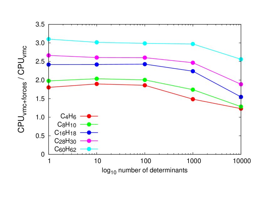
Figure 1: Ratio of the CPU time for a VMC calculation of the forces to the CPU time for the same simulation of the energy alone for the sequence of molecules C_nH_n+2 with $n$ between 4 and 60 and an increasing number of determinants in the Jastrow-Slater wave function. The forces are calculated after moving all the electrons once.

In Fig. 1, we demonstrate this favorable scaling in the variational Monte Carlo (VMC) computation of the interatomic forces for multi-determinant Jastrow-Slater wave functions using the sequence of molecules C_nH_n+2 with $n$ between 4 and 60. For each system, the ratio of the CPU time of computing all interatomic forces to the time of evaluating only the energy is initially constant and then decreases when the number of determinants exceeds about 100. For the largest C₆₀H₆₂, computing all interatomic gradients costs less than about 3 times a VMC simulation where one only evaluates the total energy. Finally, as it is shown in the Appendix, if we move one electron, many quantities can be updated so that, for each Monte Carlo step, the scaling is reduced to $O(N^{2})+O(N_{e})$. This leads to an overall scaling $O(N^{3})+O(N_{e}N)$ when all the electrons have been moved. For an all-electron-move algorithm, the scaling is $O(N^{3})+O(N_{e})$ which could be more efficient when $N_{e}$ is large.

VI Numerical results

We demonstrate the formulas above on the ground-state structural optimization in VMC of butadiene (C₄H₆) and octatetraene (C₈H₁₀) using large expansions in the determinantal component of the Jastrow-Slater wave function. All expansion coefficients, orbital and Jastrow parameters in the wave function are optimized together with the geometry. Given the large number of variational parameters (up to 58652) we employ the stochastic reconfiguration optimization method Sorella, Casula, and Rocca (2007) in a conjugate gradient implementation Neuscamman, Umrigar, and Chan (2012) which avoids building and storing large matrices. In most of our calculations, to remove occasional spikes in the forces, we use an improved estimator of the forces obtained by sampling the square of a modified wave function close to the nodes C. Attaccalite, and S. Sorella (2008). To optimize the geometry, we simply follow the direction of steepest descent and appropriately rescale the interatomic forces. We employ the CHAMP code Cha with scalar-relativistic energy-consistent Hartree-Fock pseudopotentials and the corresponding cc-pVXZ Burkatzki, Filippi, and Dolg (2007); Hps and aug-cc-pVXZ aug basis sets with X=D,T, and Q. The Jastrow factor includes two-body electron-electron and electron-nucleus correlation terms. The starting determinantal component of the Jastrow-Slater wave functions before optimization is obtained in multiconfiguration-self-consistent-field calculations performed with the program GAMESS(US) Schmidt et al. (1993); Gordon and Schmidt (2011).

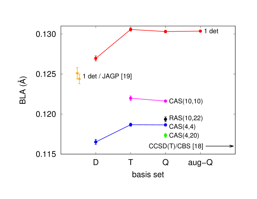
Figure 2: Bond length alternation (BLA) of C₄H₆ optimized in VMC for different basis sets and choices in the determinantal part of the Jastrow-Slater wave function. The atomic positions and all parameters of the wave function (expansion coefficients, orbital and Jastrow parameters) are simultaneously optimized. The CCSD(T) BLA in the CBS limit computed with various corrections Feller and Craig (2009) and the best value obtained with a Jastrow-antisymmetrized geminal power (JAGP) Barborini and Guidoni (2015) are reported.

Expansion	No. det	No. param.	C-C	C=C	BLA (Å)
1 det	1	1404	1.45513(12)	1.32482(05)	0.13031(16)
CAS(4,4)	20	1547	1.45211(10)	1.33347(07)	0.11865(15)
CAS(4,16)	7232	4995	1.45160(15)	1.33422(13)	0.11738(16)
CAS(4,20)	18100	9147	1.45143(16)	1.33409(07)	0.11734(24)
CAS(10,10)	15912	6890	1.45858(09)	1.33694(06)	0.12163(13)
RAS(10,22)	45644	11094	1.45705(17)	1.33760(15)	0.11945(29)
CCSD(T)/CBSa			1.4548	1.3377	0.1171
CCSD(T)/CBS-corrb			1.4549	1.3389	0.1160
a Ref. Feller and Craig, 2009; b Ref. Feller and Craig, 2009, including a CCSDT(Q)(FC)/cc-pVDZ correction.

Table 1: Optimal bond lengths and BLA values (Å) of butadiene computed in VMC with the cc-pVQZ basis set and various choices of Jastrow-Slater expansions. The numbers of determinants and optimized parameters in the wave function are listed.

We first focus on the VMC geometrical optimization of butadiene. Despite its small size and apparent simplicity, predicting the bond length alternation (BLA) of butadiene remains a challenging task for quantum chemical approaches which lead to a spread of BLA values, mainly clustered around either 0.115 or 0.125 Å (see Table 2 in Ref. Barborini and Guidoni, 2015 for a recent compilation of theoretical predictions). In particular, Barborini and Guidoni Barborini and Guidoni (2015) using VMC in combination with Jastrow-antisymmetrized geminal power (JAGP) wave functions find a best BLA value of 0.1244(6) Å, rather close to the BLA of 0.1251(7) Å they obtain using a single-determinant Jastrow-Slater wave function and clearly distinct from the CCSD(T) prediction of 0.116 Å computed in the complete basis set (CBS) limit and corrected for core-valence correlation, scalar-relativistic effects, and inclusion of quadruples Feller and Craig (2009).

To elucidate the origin of this difference, we consider here various expansions correlating the $\pi$ and $\sigma$ electrons: a) a single determinant; b) the complete-active-space CAS(4,4), CAS(4,16), and CAS(4,20) expansions (20, 7232, and 18100 determinants, respectively) of the four $\pi$ electrons in the bonding and antibonding $\pi$ orbitals constructed from the $2p_{z}$, $3p_{z}$, $3d_{xz}$, $3d_{yz}$, and $4p_{z}$ atomic orbitals; c) a CAS(10,10) correlating the six $\sigma$ and four $\pi$ electrons of the carbon atoms in the corresponding bonding and antibonding $\pi$ and $\sigma$ orbitals (15912 determinants); d) the same CAS(10,10) expansion augmented with single and double excitations in the external space of 12 $\pi$ orbitals and truncated with a threshold of 2$\times$10^-4 on the coefficients of the spin-adapted configuration state functions. This last choice results in a total of 45644 determinants and is denoted as a restricted-active-space RAS(10,22) expansion.

We start all runs from the same geometry and, after convergence, average the geometries over an additional 30-40 iterations. The results of these structural optimizations are summarized in Fig. 2. We find that the basis sets of triple- and quadruple-$\zeta$ quality yield values of BLA which are compatible within 1-1.5 standard deviations, namely, to better than 5$\times$10^-4 Å. The further addition of augmentation does not change the BLA as shown in the one-determinant case. In the following, we therefore focus on the cc-pVQZ bond lengths and BLA values of butadiene, which are summarized in Table 1.

With a one-determinant wave function (case a), we obtain a BLA of 0.1303(2) Å  which is higher than the value of 0.1251(6) Å reported in Ref. Barborini and Guidoni, 2015, possibly due to their use of a basis set of quality inferior to triple-$\zeta$. Moving beyond a single determinant, we observe a strong dependence of the result on the choice of active space. The inclusion of $\pi$-$\pi$ correlation within 4, 16, and 20 $\pi$ orbitals (case b) significantly decreases the BLA with respect to the one-determinant case with the CAS(4,16) and CAS(4,20) expansions yielding a BLA of 0.117 Å in apparent agreement with the CCSD(T)/CBS estimate of 0.116 Å. Accounting also for $\sigma$-$\pi$ and $\sigma$-$\sigma$ correlations in a CAS(10,10) (case c) leads however to a more substantial lengthening of the single than the double bond and a consequent increase of BLA. Finally, allowing excitations out of the CAS(10,10) in 12 additional $\pi$ orbitals (case d) brings the double bond in excellent agreement with the CCSD(T)/CBS value and somewhat shortens the single bond, lowering the BLA to a final value of 0.119 Å. In summary, all choices of multi-determinant expansion in the Jastrow-Slater wave function represent a clear improvement with respect to the use of a single determinant, significantly lowering the value of BLA. Consequently, the agreement reported in Ref. Barborini and Guidoni, 2015 between the single-determinant and JAGP wave functions indicates that the JAGP ansatz does not have the needed variational flexibility to capture the subtle static correlation effects in butadiene.

Finally, in Fig. 3, we demonstrate the ability of our method to optimize the structure and the many wave function parameters for the larger molecule C₈H₁₀ when using a very large determinantal expansion. For this purpose, we employ the simple cc-pVDZ basis set and consider all single, double, and triple excitations in an expansion denoted as SDT(22,22), correlating 22 electrons in the 22 $\sigma$ and $\pi$ orbitals obtained from the carbon valence atomic orbitals. The wave function comprises a total of 201924 determinants and 58652 parameters. To illustrate the dependence of the energy on the choice of wave function, we also display the energy of the last iterations of a structural optimization of the same molecule with the minimal CAS(8,8) expansion over the $\pi$ orbitals. At each iteration, we update both the wave function parameters and the atomic positions, the former with one step of the stochastic reconfiguration method and the latter along the down-hill direction of the interatomic forces. The energy of the SDT(22,22) wave function is distinctly lower than the one obtained with the smaller active space and converged to better than 2 mHartree within about 80 iterations. The structural parameters converge much faster and reach stable values within the first 30 iterations.

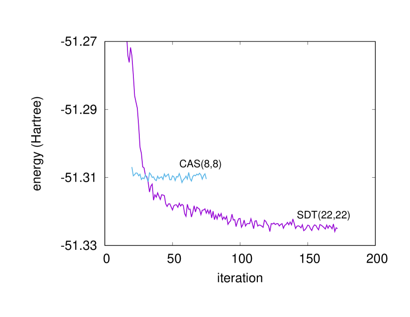
Figure 3: Total energy for a VMC geometry optimization of C₈H₁₀ using two different expansions in the Jastrow-Slater wave function, that is, a full CAS(8,8) with 2468 determinants, and all single, double, and triple excitations in an expansion correlating 22 electrons in 22 orbitals for a total of 201924 determinants. The atomic positions and all parameters of the wave function (expansion coefficients, orbital and Jastrow parameters) are simultaneously optimized.

Appendix A Efficient calculation of $Z$, $Y$, $\chi$

We demonstrate here that we do not need to compute explicitly the inverses of the submatrices $\alpha_{I}$ as in Eqs. (23, 28, and 42) or in Refs. Clark et al., 2011; Filippi, Assaraf, and Moroni, 2016 to obtain $\chi$ and its derivatives. These can be computed efficiently using recursion formulas.

Suppose that $\chi$ contains only third-order excitations (the generalization to an arbitrary order is straightforward). Let us rewrite the expression of $\chi$ (Eq. 23) as

$$\chi=\sum_{i_{1}<i_{2}<i_{3},j_{1}<j_{2}<j_{3}}C_{i_{1}i_{2}i_{3}j_{1}j_{2}j_{3}}\sum_{p}(-1)^{p}T_{i_{1}p(j_{1})}T_{i_{2}p(j_{2})}T_{i_{3}p(j_{3})}\,,$$ (46)

where $p$ stands for a permutation of the indices $(j_{1},j_{2},j_{3})$, and $(-1)^{p}$ is the sign of the permutation. We note that this formula can also include first- and second-order excitations: a second-order excitation $(i_{1}\to j_{1},i_{2}\to j_{2})$ can be written as $(i_{1},\to j_{2},i_{2}\to j_{2},i_{3}\to i_{3})$, and a first-order excitation $(i_{1}\to j_{1})$ as $(i_{1},\to j_{1},i_{2}\to i_{2},i_{3}\to i_{3})$.

The starting point is that the tensor of second derivatives can be computed directly from the expression (46) as

$$\frac{\partial^{2}\chi}{\partial T_{i_{1}j_{1}}\partial T_{i_{2}j_{2}}}=\sum_{i_{3}j_{3}}(-1)^{p+q}C_{p(i_{1})q(j_{1})p(i_{2})q(j_{2})p(i_{3})q(j_{3})}T_{i_{3}j_{3}}\,,$$ (47)

where $p$ and $q$ are the permutations ordering $(i_{1},i_{2},i_{3})$ and $(j_{1},j_{2},j_{3})$, respectively. Note that this tensor is antisymmetric with respect to the permutations of either the indices $(i_{1},i_{2})$ or the indices $(j_{1},j_{2})$, and we only need to compute and store the elements such that $i_{1}<i_{2}$, and $j_{1}<j_{2}$. The tensor of first order derivatives is

$$\frac{\partial\chi}{\partial T_{i_{1}j_{1}}}=\frac{1}{2}\sum_{i_{2}j_{2}}\frac{\partial^{2}\chi}{\partial T_{i_{1}j_{1}}\partial T_{i_{2}j_{2}}}T_{i_{2}j_{2}}\,,$$ (48)

and the value of $\chi$ is

$$\chi=\frac{1}{3}\sum_{ij}\frac{\partial\chi}{\partial T_{ij}}T_{ij}\,.$$ (49)

In practice, sparse representations of these tensors should be used. The formula (47) involves at most nine products and nine sums per excitation. The formulas (48) and (49) require less than $N^{2}N^{2}_{\rm orb}$ and $NN_{\rm orb}$ operations (additions or multiplications), respectively. The method still scales like $O(N_{e})$ but with a reduced prefactor because no divisions are involved and the number of operations is smaller. For example, expression (49) involves at most $NN_{\rm orb}$ multiplications and additions whereas (23) is a sum on $N_{e}$ terms ($N_{e}$ can be of order $N^{3}N^{3}_{\rm orb}$ if third-order excitations are included).

Appendix B One-electron-move algorithms

To sample the density $\Psi^{2}$, we use the Metropolis-Hastings method Hastings (1970); Toulouse, Assaraf, and Umrigar (2016) which is a stochastic dynamics in the space of configurations ${\bf R}=({\bf r_{1}},{\bf r}_{2}\dots\bf r_{N})$. For a given iteration, this method proposes a random move ${\bf R}\to{\bf R}^{\prime}$ with a transition probability density $P({\bf R}\to{\bf R}^{\prime})$. The proposed move is accepted with the probability

$${\rm min}\left(\frac{\Psi^{2}({\bf R}^{\prime})}{\Psi^{2}({\bf R})}\frac{P({\bf R}^{\prime}\to{\bf R})}{P({\bf R}\to{\bf R}^{\prime})},1\right)\,.$$ (50)

If only one electron is moved (here the first, for example), the new configuration is ${\bf R}^{\prime}=({\bf r_{1}}^{\prime},{\bf r}_{2}\dots\bf r_{N})$. The new extended Slater matrix $\tilde{A}^{\prime}$ differs from $\tilde{A}$ only in the first line.

We introduce the matrix $\tilde{B}_{e}$ such that the first line of $\tilde{B}_{e}$ and $\tilde{A}^{\prime}$ are the same but $\tilde{B}_{e}$ is zero elsewhere. Since $\Phi$ is a linear function of the modified line

$$\frac{\Phi{(\bf R}^{\prime})}{\Phi({\bf R})} = \partial_{\lambda}\ln\Phi(\tilde{A})\,,$$ (51)

where we considered the following transformation $\tilde{A}\to\tilde{A}+\lambda\tilde{B}_{e}$. Using Eq. (25), we obtain

$$\frac{\Phi({\bf R}^{\prime})}{\Phi({\bf R})}=\text{tr}(A^{-1}\partial_{\lambda}A)+\text{tr}(Y\partial_{\lambda}T)\,,$$ (52)

where we recall that $T=A^{-1}\tilde{A}$ and $\partial_{\lambda}T=A^{-1}\tilde{B}_{e}-A^{-1}B_{e}T$. The cost of this calculation is $O(NN_{\rm orb})\sim O(N^{2})$. When the first electron has been moved, $T$ can be updated using the Sherman Morrison formula at a cost $O(NN_{\rm orb})$Filippi, Assaraf, and Moroni (2016), and $Y$ which depends on $T$ can be again computed at a cost $O(N_{e})$. The total cost for a sweep (each electron has moved once) is $O(N^{2}N_{\rm orb})+O(NN_{e})$. The matrix $\Gamma$ and all derivatives are computed after each sweep.

We note that, if one uses instead the expression involving $\Gamma$ to update the wave function,

$$\frac{\Phi({\bf R}^{\prime})}{\Phi({\bf R})}=\text{tr}(\Gamma\tilde{B}_{e})\,,$$ (53)

one would need to update $\Gamma$ at each Monte Carlo step and incur the higher cost of $O(N^{4})+O(NN_{e})$ for a full sweep. This is because updating $\Gamma$ requires the calculation of $\partial_{\lambda}\Gamma$ given in Eq. (37), where of course $\tilde{B}$ is replaced by $\tilde{B}_{e}$. In this equation, the product $(\partial_{\lambda}Y)A^{-1}$ scales like $O(N^{3})$, unless $Y$ is sparsely modified after one electron move (i.e. a few double excitations are involved).

Finally, also in the calculation of the drift of a single electron $\nabla_{i}\Phi/\Phi$ needed in the Monte Carlo sampling, it is better not to recompute $\Gamma$ but to use formula (52) with $\partial_{\lambda}T=A^{-1}\tilde{B}^{\rm drift}_{e}-A^{-1}B^{\rm drift}_{e}T$, where the matrix $\tilde{B}^{\rm drift}_{e}$ is zero except the $i^{th}$ row which equals $\nabla\phi_{j}({\bf r}_{i})$. However, if the sampling is modified to use a finite distribution at the nodes following Ref. C. Attaccalite, and S. Sorella, 2008, the full drift has to be computed at each step. The resulting scaling is $O(N^{4})+O(NN_{e})$ per sweep, using Eq. (52) or (53) alike.

Appendix C Simple Expression of $\Gamma$ for a Jastrow-Slater expansion

Here, we provide a simple (though not efficient) expression for $\Gamma$ and some mathematical properties.

Simple expression for $\Gamma$

The determinantal contribution of the wave function written in Eq. (3) is

$$\Phi=\sum_{I=0}^{N_{e}}c_{I}\text{det}({A}_{I})\,.$$

where $A_{I}$ is a list of $N$ columns of the $N\times N_{\rm orb}$ generalized Slater matrix $\tilde{A}$. We can then define a $N_{\rm orb}\times N$ matrix $R_{I}$ such that

$$A_{I}=\tilde{A}R_{I}^{\prime}\,,$$ (54)

which gives an explicit expression of $\Phi$ as a function of $\tilde{A}$

$$\Phi(\tilde{A})=\sum_{I}c_{I}\text{det}(\tilde{A}R_{I})\,.$$ (55)

For example, given a $3\times 3$ Slater matrix built on the orbitals $(\phi_{1},\phi_{3},\phi_{4})$

$$R_{I}=\left(\begin{array}[]{cccccc}1&0&0\\ 0&0&0\\ 0&1&0\\ 0&0&1\\ 0&0&0\\ \vdots&\vdots\\ \end{array}\right)\,.$$

The derivative of the determinantal expansion with respect to a parameter $\mu$ is

$$\partial_{\mu}\Phi = \sum_{I}c_{I}\text{det}(A_{I})\text{tr}(A_{I}^{-1}\partial_{\mu}A_{I})$$

$$= \sum_{I}c_{I}\text{det}(A_{I})\text{tr}(A_{I}^{-1}\partial_{\mu}\tilde{A}R_{I})\,.$$

Using the linearity and the cyclic properties of the trace, we find

$$\frac{\partial_{\mu}\Phi}{\Phi}=\text{tr}(\Gamma\partial_{\mu}\tilde{A})\,,$$ (56)

where we can identify $\Gamma$

$$\Gamma=\frac{1}{\Phi}\sum_{I}c_{I}\text{det}(A_{I})R_{I}A_{I}^{-1}\,.$$ (57)

In the expression (57), the application of $R_{I}$ on the left of $A_{I}^{-1}$ dispatches the $N$ lines of $A_{I}^{-1}$ in a larger $N_{\rm orb}\times N$ matrix. Of course, a direct evaluation of (57) would be $O(N_{e}N^{3})$ and would be too costly.

Properties of the matrix $\Gamma$

$\Gamma$ is a right inverse of $\tilde{A}$, i.e.

$$\tilde{A}\Gamma=I_{N}\,,$$ (58)

where $I_{N}$ is the identity matrix of order $N$. The proof is simple

$$\tilde{A}\Gamma = \frac{1}{\Phi}\sum_{I}c_{I}\text{det}(A_{I})\tilde{A}R_{I}A_{I}^{-1}$$ (59)

$$= \frac{1}{\Phi}\sum_{I}c_{I}\text{det}(A_{I})A_{I}A_{I}^{-1}=I_{N}\,.$$ (60)

We now consider the $N_{\rm orb}\times N_{\rm orb}$ matrix $\Gamma\tilde{A}$ and resort to the transformation $\phi_{i}\to\phi_{i}+\mu_{ij}\phi_{j}$. The only non-zero column of the matrix ${\partial\tilde{A}}/{\partial\mu_{ij}}$ is the $i^{th}$ column, which is the same as the $j^{th}$ column of $\tilde{A}$. Therefore,

$$\frac{1}{\Phi}\frac{\partial\Phi}{\partial\mu_{ij}}=\text{tr}\left(\Gamma\frac{\partial\tilde{A}}{\partial\mu_{ij}}\right)=(\Gamma\tilde{A})_{ij}\,,$$ (61)

meaning that $\Phi(\Gamma\tilde{A})_{ij}$ is the new value of the determinantal expansion when the orbital $i$ has been replaced by the orbital $j$

$$\Phi(\Gamma\tilde{A})_{ij}=\sum_{I}c_{I}\text{det}(A_{I}^{i\to j})\,.$$ (62)

In particular, if $i=j$,

$$\Phi(\Gamma\tilde{A})_{ii}=\sum_{I/\phi_{i}\in A_{I}}c_{I}\text{det}(A_{I})\,.$$ (63)

In other words, the main diagonal of $\Phi\Gamma\tilde{A}$ is made of restrictions of the summation in (3) to determinants containing a given orbital. As a by-product, if $\phi_{i}$ is common to all the determinants of the expansion, $(\Gamma\tilde{A})_{ii}$ is equal to $1$. If $i\neq j$, $\Phi(\Gamma\tilde{A})_{ij}$ is the expansion (3) restricted to Slater determinants occupied by $\phi_{i}$ and not by $\phi_{j}$

$$\Phi(\Gamma\tilde{A})_{ij}=\sum_{I/\phi_{i}\in A_{I},\Phi_{j}\not\in A_{I}}c_{I}\text{det}(A_{I}^{i\to j})\,.$$ (64)

In particular, if the orbital $j$ is common to all determinants, $(\Gamma\tilde{A})_{ij}=0$ for any $i\neq 0$. In conclusion, if there are $N_{\rm act}$ orbitals which can be excited (i.e. there are $N-N_{\rm act}$ orbitals common to all determinants), the following property holds: $\Gamma\tilde{A}$ contains a $N_{\rm orb}\times(N-N_{\rm act})$ block which is zero with the exception of a $(N-N_{\rm act})\times(N-N_{\rm act})$ square sub-block which is the identity matrix.

Appendix D Calculation of $\Gamma$ using the Sherman-Morrison-Woodbury formula

Here, we derive the expression (30) directly from the identity (57) using the Sherman-Morrsion-Woodbury formula. The algebra is a bit more tedious. First, we remind some notations useful to explicit the matrix $R_{I}$ and dependencies on $\tilde{A}$. $A$ is the reference Slater matrix and $R$ is the matrix which selects the columns $\tilde{A}$ from which $A$ is made

$$A=\tilde{A}R\,.$$ (65)

$P_{I}$ is the matrix such that $AP_{I}$ is the list of the $k_{I}$ columns of $A$ which differ from those of $A_{I}$ (see for example Eq. (19)). The $N\times N$ matrix $P_{I}P_{I}^{T}$ is a diagonal matrix: if $i$ is the index of a column which differ in $A$ and $A_{I}$, $(P_{I}P_{I}^{T})_{ii}=1$, while $(P_{I}P_{I}^{T})_{ii}=0$ otherwise. Consequently, the identity

$$A_{I}-A=(A_{I}-A)P_{I}P_{I}^{T}$$ (66)

holds. The list of excited orbitals are the columns of $A_{I}P_{I}$ and can be selected from $\tilde{A}$ with the aid of the $N_{\rm orb}\times k_{I}$ matrix $Q_{I}$ such that

$$A_{I}P_{I}=\tilde{A}Q_{I}\,,$$ (67)

as in the example Eq. (20). With these definitions

$$A_{I}=A+(A_{I}-A)P_{I}P_{I}^{T}=\tilde{A}\left(R+(Q_{I}-RP_{I})P_{I}^{T}\right)\,,$$ (68)

and the matrix $R_{I}$ which selects the columns $\tilde{A}$ from which $A_{I}$, is given by

$$R_{I}=R+(Q_{I}-RP_{I})P_{I}^{T}\,.$$ (69)

Now, writing $A_{I}=A+(A_{I}-A)P_{I}P_{I}^{T}$ and applying the Sherman-Morrison-Woodbury formula, we obtain

$$A_{I}^{-1} = A^{-1}-A^{-1}(A_{I}-A)P_{I}(1+P_{I}^{T}A^{-1}(A_{I}-A)P_{I})^{-1}\,P_{I}^{T}A^{-1}$$ (70)

$$= A^{-1}-A^{-1}(A_{I}-A)P_{I}(P_{I}^{T}A^{-1}A_{I}P_{I})^{-1}\,\,P_{I}^{T}A^{-1}\,,$$

so that

$$A_{I}^{-1}=A^{-1}+P_{I}\alpha_{I}^{-1}P_{I}^{T}A^{-1}-A^{-1}\tilde{A}Q_{I}\alpha_{I}^{-1}P_{I}^{T}A^{-1}\,,$$ (71)

where we have introduced

$$\alpha_{I}\equiv P_{I}^{T}A^{-1}\tilde{A}Q_{I}\,.$$ (72)

Multiplying both sides of Eq. (71) by $P_{I}^{T}$ gives the following identity

$$P_{I}^{T}A_{I}^{-1} = P_{I}^{T}P_{I}\alpha_{I}^{-1}\,\,P_{I}^{T}A^{-1}$$ (73)

$$= \alpha_{I}^{-1}\,\,P_{I}^{T}A^{-1}\,.$$

Using this expression, we can simplify

$$R_{I}A_{I}^{-1} = RA_{I}^{-1}+(Q_{I}-RR_{I})\alpha_{I}^{-1}\,\,P_{I}^{T}A^{-1}$$ (74)

$$= RA^{-1}-RA^{-1}\tilde{A}Q_{I}\alpha_{I}^{-1}P_{I}^{T}A^{-1}+Q_{I}\alpha_{I}^{-1}P^{T}_{I}A^{-1}$$

$$= RA^{-1}+(1-RA^{-1}\tilde{A})Q_{I}\alpha_{I}^{-1}P_{I}^{T}A^{-1}$$

From equations (74) and (57), we then obtain

$$\Gamma=RA^{-1}+\ (1-RA^{-1}\tilde{A})YA^{-1}\,,$$ (75)

with

$$Y\equiv\frac{\text{det}(A)}{\Phi}\sum_{I}c_{I}\text{det}(\alpha_{I})Q_{I}\alpha_{I}^{-1}P_{I}^{T}$$ (76)

and, of course,

$$\Phi = \text{det}(A)\left(\sum_{I=1}^{N_{e}}c_{I}\text{det}(\alpha_{I})\right)\,.$$ (77)

References

• Umrigar et al. (2007) C. J. Umrigar, J. Toulouse, C. Filippi, S. Sorella,  and R. G. Hennig, Phys. Rev. Lett. 98, 110201 (2007).
• Sorella and Capriotti (2010) S. Sorella and L. Capriotti, J. Comp. Phys. 133, 234111 (2010).
• Filippi, Assaraf, and Moroni (2016) C. Filippi, R. Assaraf,  and S. Moroni, The Journal of Chemical Physics 144, 194105 (2016), http://dx.doi.org/10.1063/1.4948778.
• Clark et al. (2011) B. K. Clark, M. A. Morales, J. McMinis, J. Kim,  and G. E. Scuseria, J. Chem. Phys. 135, 244105 (2011).
• Assaraf and Caffarel (1999) R. Assaraf and M. Caffarel, Phys. Rev. Lett. 83, 6482 (1999).
• Filippi and Umrigar (2000) C. Filippi and C. J. Umrigar, Phys. Rev. B 61, R16291 (2000).
• Assaraf and Caffarel (2003) R. Assaraf and M. Caffarel, J. Chem. Phys. 119, 10536 (2003).
• Note (1) Or $O(N^{3})+O(N^{2}N_{\rm act}N_{\rm atoms})+O(N_{e}N_{\rm atoms})$.
• Sorella, Casula, and Rocca (2007) S. Sorella, M. Casula,  and D. Rocca, J. Chem. Phys. 127, 014105 (2007).
• Neuscamman, Umrigar, and Chan (2012) E. Neuscamman, C. J. Umrigar,  and G. K.-L. Chan, Phys. Rev. B 85, 045103 (2012).
• C. Attaccalite, and S. Sorella (2008) C. Attaccalite, and S. Sorella, Phys. Rev. Lett. 100, 114501 (2008).
• (12) CHAMP is a quantum Monte Carlo program package written by C. J. Umrigar, C. Filippi, S. Moroni and collaborators.
• Burkatzki, Filippi, and Dolg (2007) M. Burkatzki, C. Filippi,  and M. Dolg, J. Chem. Phys. 126, 234105 (2007).
• (14) For the hydrogen atom, we use a more accurate BFD pseudopotential and basis set. Dolg, M.; Filippi, C., private communication.
• (15) We take the diffuse functions from the aug-cc-pVXZ basis sets in the EMSL Basis Set Library (http://bse.pnl.gov). We do not include the g functions in the cc-pVQZ and aug-cc-pVQZ basis sets.
• Schmidt et al. (1993) M. W. Schmidt, K. K. Baldridge, J. A. Boatz, S. T. Elbert, M. S. Gordon, J. H. Jensen, S. Koseki, N. Matsunaga, K. A. Nguyen, S. Su, T. L. Windus, M. Dupuis,  and J. A. M. Jr, J. Comput. Chem. 14, 1347 (1993).
• Gordon and Schmidt (2011) M. S. Gordon and M. W. Schmidt, in Theory and Applications of Computational Chemistry: the first forty years, edited by C. Dykstra, G. Frenking, K. Kim,  and G. Scuseria (Elsevier, Amsterdam, 2011) Chap. 41, pp. 1167–1190.
• Feller and Craig (2009) D. Feller and N. C. Craig, The Journal of Physical Chemistry A 113, 1601 (2009).
• Barborini and Guidoni (2015) M. Barborini and L. Guidoni, Journal of Chemical Theory and Computation 11, 508 (2015).
• Hastings (1970) W. K. Hastings, Biometrika 57, 97 (1970)http://biomet.oxfordjournals.org/cgi/reprint/57/1/97.pdf .
• Toulouse, Assaraf, and Umrigar (2016) J. Toulouse, R. Assaraf,  and C. J. Umrigar, Advances in Quantum Chemistry 73, 285 (2016).