Ordered Line Integral Methods
for Computing the Quasi-potential
Abstract
The quasi-potential is a key function in the Large Deviation Theory. It characterizes the difficulty of the escape from the neighborhood of an attractor of a stochastic non-gradient dynamical system due to the influence of small white noise. It also gives an estimate of the invariant probability distribution in the neighborhood of the attractor up to the exponential order. We present a new family of methods for computing the quasi-potential on a regular mesh named the Ordered Line Integral Methods (OLIMs). In comparison with the first proposed quasi-potential finder based on the Ordered Upwind Method (OUM) (Cameron, 2012), the new methods are 1.5 to 4 times faster, can produce error two to three orders of magnitude smaller, and may exhibit faster convergence. Similar to the OUM, OLIMs employ the dynamical programming principle. Contrary to it, they have an optimized strategy for the use of computationally expensive triangle updates leading to a notable speed-up, and directly solve local minimization problems using quadrature rules instead of solving the corresponding Hamilton-Jacobi-type equation by the first order finite difference upwind scheme. The OLIM with the right-hand quadrature rule is equivalent to OUM. The use of higher order quadrature rules in local minimization problems dramatically boosts up the accuracy of OLIMs. We offer a detailed discussion on the origin of numerical errors in OLIMs and propose rules-of-thumb for the choice of the important parameter, the update factor, in the OUM and OLIMs. Our results are supported by extensive numerical tests on two challenging 2D examples.
Keywords: Quasi-potential; Ordered Line Integral Methods; Ordered Upwind Method; Accuracy; CPU time; Update radius; Hierarchical Update Strategy
MSC 2010 Numbers: 65N99; 49L20; 60J60
1 Introduction
The quasi-potential is a key concept of Large Deviation Theory [6]. Let us consider a nongradient stochastic differential equation (SDE) of the form
| (1) |
where is a twice continuously differentiable vector field, is the standard -dimensional Brownian motion, and is a small parameter. We assume that the corresponding deterministic system has a finite number of attractors. Let be an attractor and be a point. The quasi-potential at with respect to the attractor can be defined as (details are provided in Appendix A)
| (2) |
In Eq. (2), is the 2-norm, the functional is the geometric action [8, 9], is an absolutely continuous path from to parametrized by its arc length (i.e., ), is its length which can be infinite. According to the Large Deviation Theory, the expected first passage time from a small neighborhood of the attractor to a small neighborhood of the point lying in its basin of attraction is logarithmically equivalent to [6]. The curve corresponding to the maximum likelihood path to from is the global minimizer of the geometric action [6, 8, 9]. The invariant probability distribution in the basin of attraction of is logarithmically equivalent to [6]. A nice and visual account on the significance of the quasi-potential as a tool for quantifying the stability of attractors is found in [14].
Nongradient SDEs of the form (1) often arise in modeling of ecological and biological systems. A number of models of population dynamics were analyzed in [14] using the quasi-potential. The quasi-potential for a genetic switching model was constructed in [12].
Therefore, the quasi-potential is of crucial importance for the quantification of the dynamics of systems evolving according to SDE (1) with a small noise. Unfortunately, it is not readily available for nongradient SDEs and can be found analytically only in special cases. For example, analytic formulas for the quasi-potential are available for linear SDEs [1, 3]. For general nonlinear SDEs, finding the quasi-potential is a difficult task. In any bounded neighborhood of an attractor of , the quasi-potential is a Lipschitz-continuous but not necessarily differentiable function as it is for the Maier-Stein [13, 1] model. One can show that the quasi-potential , i.e., the solution of the functional minimization problem (2), is also a viscosity solution of a Hamilton-Jacobi-type PDE [1]
| (3) |
Eq. (3) has at least two viscosity solutions due to the fact that is an attractor and for all : and is the quasi-potential (i.e, the solution of Eq. (2)). We refer an interested reader to Refs. [5] and [11] where the concept of viscosity solution was introduced and the questions of existence and uniqueness of solution of Eq. (3) were investigated respectively.
1.1 Background
Minimum Action Paths (MAPs), i.e., minimizers of the geometric action ((Eq. (2)) can be found numerically by path-based methods. The Geometric Minimum Action Method (GMAM) [8, 9] and the Adaptive Minimum Action Method (AMAM) [21, 22] iteratively update paths connecting given initial and final points starting from user-provided initial guesses so that the paths approach a local minimizer of the geometric action (Eq. (2)) and a local minimizer of the original Freidlin-Wentzell action (Eq. (A-1)) respectively. The advantage of the path-based methods is that they are suitable for high- and even infinite-dimensional systems, i.e., stochastic partial differential equations (SPDEs) (e.g., [8, 7]). However, the found action minimizer is biased by the initial path and hence might not be the global minimizer, and it can be inexact due to slow convergence of the iterative process and numerical effects in the case if the actual MAP exhibits complex behavior. If the global action minimizer is found, the quasi-potential can be calculated along it.
Finding the quasi-potential in the whole region surrounding the attractor has important advantages over the search for MAPs. First, the quasi-potential allows us to estimate the invariant probability density near the attractor up to exponential order [6, 1]. Second, suppose a system has more than two attractors. Once the quasi-potential is computed with respect to an attractor in a large enough region, the most likely escape set from the basin of attraction of is automatically detected as the quasi-potential is constant along any trajectory running from to another attractor. The escape set can be a saddle point, a hyperbolic periodic orbit, or a more complex set of points in the phase space. Once the quasi-potential is computed, the global minimizer of the geometric action connecting the attractor with the escape set is guaranteed to be found by straightforward numerical integration [1] (see Section 3, Fig. 4 and its caption). On the contrary, path-based methods might have wrong endpoints, e.g., the most likely escape from is to the attractor , while a path-based method is set up to seek action minimizers connecting attractors and . Furthermore, even if the endpoints are identified correctly, path-based methods might converge to local minimizers.
On the other hand, it is clear that the computation of the quasi-potential in whole regions of the phase space is limited to low-dimensional systems.
To the best of our knowledge, the first attempt to compute the quasi-potential on a regular mesh was undertaken in [1]. It was done for 2D systems for both possible types of attractors, asymptotically stable equilibrium and stable limit cycle. The proposed numerical technique was an adjustment of the Ordered Upwind Method (OUM) [17, 18] for the case where the anisotropy coefficient was unbounded. (What is the anisotropy coefficient will be explained right below.) The original OUM was designed for solving Hamilton-Jacobi equations of the form , where , with the boundary condition where can be a point or a curve. The function , the speed of front propagation in the normal direction, was assumed to be bounded: . The Hamiltonian was assumed to be convex, Lipschitz-continuous, and homogeneous of degree one in . The anisotropy coefficient is the ratio of the maximal and the minimal values of the speed function: . One can think of being the minimal possible travel time from to the point in the following associated control problem. Suppose an astronaut on Mars (a 2D manifold with no roads) needs to minimize his traveltime from to . He can pick the direction of motion of his rover at every moment of time. The speed of the rover is the function of the position and the direction of motion . The speed functions and relate via a Legendre transform. We refer an interested reader to Ref. [18].
The OUM [17, 18] employs the dynamical programming principle, i.e., at each step it solves the driver’s optimal control program by means of a finite difference upwind scheme for . The role of the anisotropy coefficient is very important. The value of at a mesh point can be updated only from the mesh points lying within the distance of from it (, , are the mesh steps in and respectively).
Eq. (3), the Hamilton-Jacobi equation for the quasi-potential, can be put in the form :
| (4) |
Hence, the front speed function is . The corresponding speed function is the integrand in Eq. (2). It is clear that the speed function is unbounded at any direction at the points where , and at the directions normal to at any point where . This difficulty was overcome in [1] by the introduction of the update factor ( is a positive integer) such that the value of at a mesh point could be updated only from the mesh points lying within the distance of (i.e., within the update radius ) from it. The additional numerical error due to this adjustment was investigated [1] and shown to decay quadratically for a fixed update radius with mesh refinement. The OUM for finding the quasi-potential was incorporated into an R-package QPot available at cran.r-project.org [15, 16].
1.2 A brief summary of main results
In this paper, we present a new family of methods for computing the quasi-potential on a regular rectangular mesh.
Like the OUM, these methods are based on the dynamical programming principle. Contrary to OUM, they
do not use the upwind scheme for solving local minimization problems. Moreover, they completely abandon Hamilton-Jacobi Eq. (3)
and refer only to the minimization problem (2).
At each step, the local minimization problem is solved on the set of local straight line paths
of length at most 111 Daisy Dahiya: ddahiya@math.umd.edu;
Maria Cameron cameron@math.umd.edu;
Department of Mathematics, University of Maryland, College Park, MD 20742.
The Lagrangian
is integrated along them using quadrature rules.
Therefore, we name this family of methods the Ordered Line Integral Methods.
The names of the methods in this family reflect which quadrature rule is
employed:
| OLIM-R: | Right-hand rectangle rule; |
| OLIM-MID: | Midpoint rule; |
| OLIM-TR: | Trapezoid rule; |
| OLIM-SIM: | Simpson’s rule. |
We prove a theorem showing that the solution of the minimization problem in OLIM-R method is equivalent to the solution of the upwind scheme in the OUM. Our extensive numerical experiments with the other OLIMs show that they are significantly more accurate than the OUM. Our least squares fits to the error formula indicate that their error constants are up to 100 times smaller and the exponents are larger than those for OUM and OLIM-R. To make sure, OLIMs like OUM are at most first order due to the use of linear interpolation, but the major portion of the numerical error, the quadrature rule error, decays at least quadratically with the mesh refinement, which affects the exponents (makes them greater than 1) obtained by the least squares fits. Furthermore, we propose a CPU-time-saving implementation for OLIMs that reduces the number of calls of computationally expensive triangle update. As a result, the OLIM-R is about four times faster than the OUM. The other OLIMs are also faster than the OUM by some more modest factors. The graphs of the CPU times versus errors eloquently display that the OLIMs with second and higher order quadrature rules produce at least as accurate solutions as the OLIM-R (and hence the OUM) at smaller by several orders of magnitude CPU times.
So far, we have implemented the OLIMs in 2D. Our C codes OLIM_righthand.c, OLIM_midpoint.c, OLIM_trapezoid.c and OLIM_simpson.c are posted on M. Cameron’s web site [2]. A promotion of OLIMs to 3D in underway and will be reported elsewhere in the future.
2 Ordered Line Integral Methods
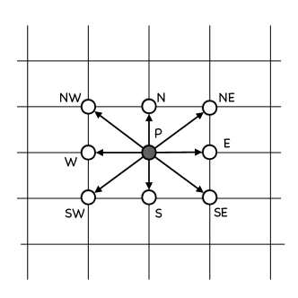
Throughout the rest of the paper, we will assume that the attractor of the system under consideration is fixed and omit the subscript in the notation for the quasi-potential with respect to : . We consider a regular rectangular mesh with mesh steps and in and directions respectively, and set . The mesh defines the sets of nearest neighbors for each mesh points. Every inner mesh point has eight nearest neighbors surrounding it as shown in Fig. 1
Similar to as it is done in the OUM [17, 18, 1], the mesh points are divided into the following four categories.
-
0.
Unknown points: the points where the solution has not been computed yet, and none of its nearest neighbors is Accepted or Accepted Front.
-
1.
Considered: the points that have Accepted Front nearest neighbors. Tentative values of that might change as the algorithm proceeds, are available at them.
-
2.
Accepted Front: the points at which has been computed and no longer can be updated, and they have at least one Considered nearest neighbor.
-
3.
Accepted: the points at which has been computed and no longer can be updated, and they have only Accepted and/or Accepted Front nearest neighbors.
The general outline of the OLIMs coincides with the one of the OUM.
Initialization
Start with all mesh points being Unknown.
Compute tentative values of at mesh points near the attractor and make them Considered.
The main body
while the boundary of the mesh is not reached and the set of Considered points is not empty
1: Make the Considered point with the smallest tentative value of Accepted Front.
2: Make all Accepted Front nearest neighbors of that no longer have Considered nearest neighbors Accepted.
3: Update all Considered points within the distance from using and maybe its nearest Accepted Front neighbors.
4: Make all Unknown nearest neighbors of Considered and compute tentative values of at them using the
Accepted Front points lying within the distance from them.
end while
In the rest of this section, we will elaborate the initialization and steps 3 and 4 of the while-cycle.
2.1 Initialization
The way the initialization is performed is important for the accuracy of the computation of the quasi-potential. The two types of attractors in 2D, the asymptotically stable equilibrium point and the asymptotically stable limit cycle, correspond to the boundary condition given at an initial point or curve respectively. The initialization procedure depends on whether the computation starts from the initial point or the initial curve.
2.1.1 Initialization from the initial point
Let be an asymptotically stable equilibrium of . Since is twice continuously differentiable and , we get
| (5) |
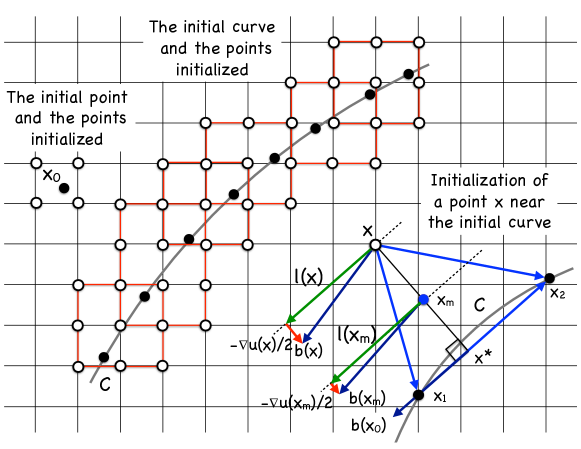
in the neighborhood of . We calculate the quasi-potential for the linear approximation at the four mesh points surrounding the point (Fig. 2, Left) using the analytic formula [1] for the quasi-potential for a linear SDE with an asymptotically stable equilibrium. Let , , , and be the entries of the matrix in Eq. (5). Then the quasi-potential in the neighborhood of is approximated by
| (8) | ||||
| (9) | ||||
These four mesh points surrounding the point become Considered.
2.1.2 Initialization from the initial curve
The initialization of the mesh points in the neighborhood of the initial curve is based on the observation that the gradient of the quasi-potential vanishes at (see Fig. 2, Center and Right). Assuming that is a smooth curve, there is a neighborhood of where the gradient of the quasi-potential is a smooth vector field. Hence, in , the following decomposition into two smooth vector fields takes place:
| (10) |
One can easily deduce this decomposition using Eq. (3). Since the rotational component is smooth, its direction in changes continuously and can be approximated by the direction of at the orthogonal projection of onto the curve . Taking into account that vanishes at and therefore
| (11) |
we approximate the gradient of the quasi-potential in by
| (12) |
The second term in the right-hand side of Eq. (12) is the projection of onto . The curve is provided by the user by a set of points . It is assumed that , , and are consecutive points along the curve. We define for , and . For each pair of the consecutive points along the curve , we define the smallest rectangle containing and with sides lying on the mesh lines and denote it by . A collection of such rectangles is shown in Fig. 2, Center, by red contours. We will initialize all mesh points lying in the union of the rectangles
| (13) |
Each mesh point located within is initialized using Simpson’s quadrature rule as follows. First, observe that for any pair of points and we have
| (14) |
Let us take , the point to be initialized, and , the projection of onto the curve . Note that and . An approximation to is constructed as follows. Let be the closest point of the curve to the point , and the point be the neighboring point of along the curve such that the angle between the vectors and does not exceed (Fig. 2, Right). The projection is approximated by the orthogonal projection of onto the line passing through and :
To use Simpson’s rule for computing the integral in Eq. (14), we need to evaluate , , , and , where is the midpoint between and . Since and on , and . Next, we note that on the line segment , is nearly parallel to , hence . Finally, we approximate and using Eq. (12) and get
| (15) |
All initialized mesh points become Considered.
2.2 The one-point updates and the triangle updates
The OUM [17, 18, 1] involves two types of updates: the one-point update and the triangle update. The OUM one-point update applied to (3) reads
| (16) | ||||
where is the mesh point being updated and is an Accepted Front point within the distance from . Eq. (16) is merely the integrand in Eq. (2) integrated along the line segment from to using the right-hand rectangle quadrature rule. The OUM triangle update is done by the upwind finite difference scheme applied to PDE (3). Its details are worked out in Section 2.3 below.
In the proposed OLIMs, the finite difference scheme as well as PDE (3) are completely abandoned. The one-point update and the triangle update are done as follows. Let be a basic quadrature rule, i.e., right-hand rectangle, midpoint, trapezoid, or Simpson’s. The OLIM one-point update results from the application of for the integration of the integrand of Eq. (2) along the line segment :
| (17) |
I.e., we compute the value and replace the current value of at with if and only if it is smaller than the current value. The OLIM triangle update at the mesh point from the triangle , where the points and are assumed to be nearest neighbors, results from solving the minimization problem
| (18) | ||||
where the vector field is approximated with a linear field within the triangle for the purpose of the application of the quadrature rule. The minimization problem (18) is solved by taking the derivative of the function to be minimized, setting it to zero, i.e.,
and then trying to find a root of in the interval . For this purpose, we use the hybrid secant/bisection method [20, 19].
Depending on the quadrature rule used, we denote the methods OLIM-R, OLIM-MID, OLIM-TR, and OLIM-SIM (see Section 1). The details of the triangle update for each OLIM are worked out in Appendix B.
2.3 Equivalence of update rules in the OUM and OLIM-R
The one-point update in OLIM-R and the OUM are done according to Eq. (16). In this section, we show that the triangle updates in OLIM-R and the OUM, if successful, give identical results.
The triangle update in the OUM [1] is done as it is proposed in [18]. The quasi-potential is assumed to be linear within the triangle and have Accepted values and at and respectively (see Fig. 13). Its value at is to be found. The finite-difference scheme proposed in [17, 18] applied to Eq. (3) is derived from the observation that
| (19) |
where , , and are the values of at the points , , and respectively. The vector field within the triangle is approximated by the constant field ( evaluated at ). Throughout the rest of this section, we will omit the argument of . Denoting the matrix on the right-hand side of Eq. (19) by and plugging into Eq. (3), we obtain the following quadratic equation for :
| (20) |
If Eq. (20) has a solution satisfying , it is subjected to the consistency test that the characteristic passing through the point crosses the segment . The direction of the characteristic is given by [1]. The condition that it crosses the segment is equivalent to the fact that is a linear combination with nonnegative coefficients , , i.e., the vector
| (21) |
has nonnegative entries. If has passed the consistency test then .
OLIM-R performs the triangle update by solving the following minimization problem
| (22) | |||
Like Eq. (20), Eq. (22) is set up under the assumption that the function is linear within the triangle .
The solution by the finite difference scheme (20) and the solution of the minimization (22) are equivalent in the sense specified by the following theorem.
Theorem 1.
The proof of Theorem 1 is given in Appendix C.
2.4 Reducing CPU time: a hierarchical update strategy
(a)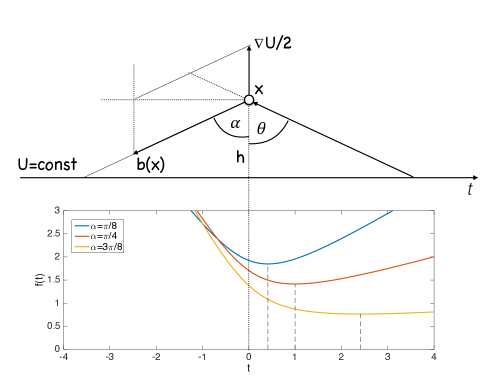
(b)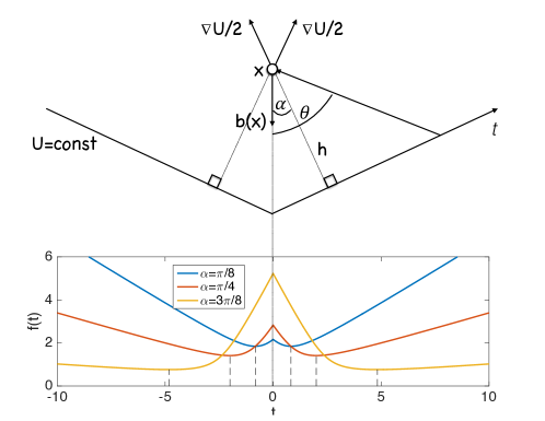
Clearly, the one-point updates require significantly fewer floating point operations than the triangle updates in both the OUM and the OLIMs. Therefore, we want to develop of a strategy for reducing the number of calls for the triangle update. Suppose that the mesh is fine enough so that is approximately constant within the update radius , and level sets of can be approximated by line segments within the distance from the mesh point to be updated.
Motivated by this, we consider the following idealized situation. Let be constant and the level set be a straight line. Let be a point at the distance from this level set as shown in Fig. 3 (a,Top). Then
where is the axis along the level set, and is the update function
| (23) |
The angles and are defined as shown in Fig. 3 (a, Top). Differentiating with respect to , setting its derivative to zero, and then returning to the variable , we find that has a single minimum on achieved at (see Fig. 3 (a, Bottom)).
Now we address the case where the quasi-potential is not differentiable along some curve, and hence its level sets have kinks. Typically, the vector field at the kink curve is directed approximately toward the kink. For example, see the quasi-potential computed in Ref. [1] for the Maier-Stein model [13]. To account for such a case, we consider the following idealized situation. Let be constant, and the level set consists of two line segments. Let be the arclength parameter along the level set, at the kink, and the angles and be defined as shown in Fig. 3 (b, Top). Let the point lie on the kink line. The update function for this case is obtained from the one in Eq. (23) using an appropriate reflection. Its graphs for three values of are shown in Fig. 3 (b, Bottom). It has two local minima at .
These considerations suggest that the update values of at a Considered point lying near the Accepted Front as functions of an arclength parameter along the level set of approximating the Accepted Front will behave similar to the graphs in Fig. 3(a, Bottom, or b, Bottom), i.e., have a single local minimum, or two equal local minima. Therefore, we have rationalized the update procedures as follows. When step 4 of the main body of the algorithm is performed, i.e., an Unknown nearest neighbor of the new Accepted Front point becomes Considered, we compute tentative values at from every Accepted Front point at distance at most from using only the cheap one-point update. Suppose the minimal tentative value at by the one-point update has been computed from the Accepted Front point , i.e.,
Only then the triangle updates are called for all Accepted Front nearest neighbors of (if any). Then
The symbol denotes the set of the nearest neighbors of (eight nearest neighbors for every inner point as shown in Fig. 1). We will refer to this update strategy as the hierarchical update strategy.
Our numerical experiments in Section 3 below indicate that this strategy reduces CPU time in OLIM-R in comparison with the OUM by the factor of approximately 4, while the numerical errors in them either coincide, or the ones in OLIM-R exceed the ones in the OUM by less than 1%.
3 Numerical tests
We compare performances of the OLIMs (OLIM-R, OLIM-MID, OLIM-TR, and OLIM-SIM) and the original OUM-based [1] quasi-potential solver on two examples for which analytic formulas for the quasi-potential are available. These two examples are quite challenging from the computational point of view due to the large rotational components of in comparison with and large curvatures of their MAPs (Minimum Action Paths). Furthermore, in the second example, the quasi-potential grows as a fourth degree polynomial.
A linear SDE. For the linear SDE [1]
| (24) |
the quasi-potential with respect to the origin, the asymptotically stable equilibrium of the corresponding deterministic system, is the quadratic function
| (25) |
The parameter is the quotient of the magnitudes of the rotational and the potential components ( and respectively) of the vector field :
| (26) |
We set , i.e., the rotational component exceeds the potential component in magnitude by the factor of 10 that makes the computation of the quasi-potential challenging. The computational domain for this example is the square . The Minimum Action Path for SDE (24) arriving at the point is shown in Fig. 4(a).
An SDE with a limit cycle. The unit circle is the asymptotically stable limit cycle of the deterministic system corresponding to the SDE [10, 1]
| (27) |
The quasi-potential with respect to the unit circle is given by the quartic function111Actually, in our codes, the maximal update length for the one-point update is , while it is for the triangle update.
| (28) |
The decomposition of the vector field into the potential and the rotational components is
| (29) |
We set the computational domain for this example to be the square . The Minimum Action Paths for SDE (24) arriving at the points and are shown in Fig. 4(b).
(a)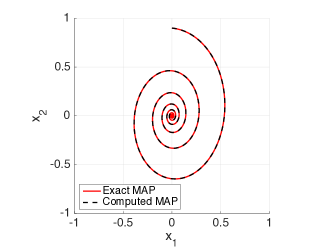 (b)
(b)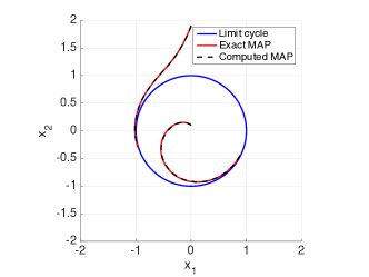
We test the OLIMs and the OUM on SDEs (24) and (27). The mesh sizes are where , . The update factor varies from to . We have measured the maximum absolute error, the RMS error, and the CPU time for each mesh size and for each value of .
3.1 Dependence of the accuracy on the update factor
The choice of the optimal value of the update factor is a subtle issue. On one hand, if the Minimum Action Paths (MAPs) for a considered SDE would be straight lines, large would enable all mesh points to be updated from the correct triangles and hence enhance the accuracy. However, typically, MAPs are not straight lines. Furthermore, large leads to numerical integration by simple quadrature rules along long linear segments and hence increases the integration error. Finally, large increases the CPU time. As a result, the optimal should be not too large and not too small.
The results of our measurements are shown in Fig. 5. For all methods, and all mesh sizes , we plot the maximal absolute error versus for SDEs (24) and (27). Note that the optimal values of are larger for SDE (24) than those for SDE (27).
Based on our plots, we propose the following Rules-of-Thumb for choosing . The points of the graphs corresponding to the proposed Rules-of-Thumb are marked on the graphs by large dots.
The Rule-of-Thumb for the OUM and OLIM-R. For an mesh where , pick
| (30) |
The Rule-of-Thumb for OLIM-MID, OLIM-TR, and OLIM-SIM. For an mesh where , pick
| (31) |
(a)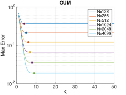 (b)
(b)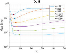
(c)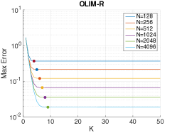 (d)
(d)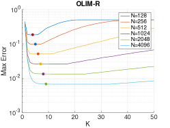
(e)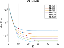 (f)
(f)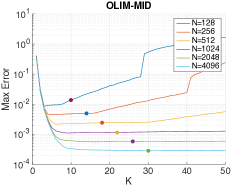
(g)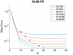 (h)
(h)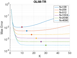
(i)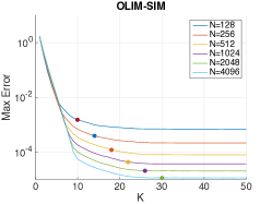 (j)
(j)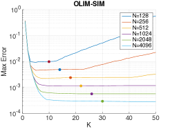
3.2 Comparison of OLIM-MID, OLIM-TR, and OLIM-SIM to OLIM-R and the OUM
Our comparison of OLIM-MID, OLIM-TR, and OLIM-SIM to OLIM-R and the OUM is unambiguously in favor of the former ones. The comparison is conducted using the update factor according to the Rule-of-Thumb for the OUM and OLIM-R, i.e., in the way benefiting the OUM and OLIM-R rather than the OLIMs with higher order quadrature rules.
The graphs of the maximum absolute error and the CPU time as functions of respectively are shown in Fig. 6 (a,b,c,d). The least squares fits to the formulas and for the maximum absolute errors and the CPU times respectively are given in Table 1. Fig. 6 (a,b) and Table 1 (Columns 2 and 4) show that OLIM-MID, OLIM-TR, and OLIM-SIM are 100 to 1000 times more accurate then OLIM-R and the OUM for values of optimized for the latter methods. Fig. 6 (c,d) and Table 1 (Columns 3 and 5) show that OLIM-MID, OLIM-TR, and OLIM-SIM are faster than the OUM. OLIM-MID is faster than the OUM at least by the factor of 1.5. OLIM-R is faster than the OUM at least by the factor of 3. The CPU time (in seconds) versus the update factor for is plotted for the OLIMs and the OUM in Fig. 7. These plots illustrate the advantage of our time-saving update strategy.
The CPU time as the function of the maximum absolute error is plotted in Fig. 6. It is clear that OLIM-MID, OLIM-TR, and OLIM-SIM are significantly better methods than OLIM-R and the OUM in terms of the balance between the accuracy and the CPU time.
| Method | Max Error | CPU time | Max Error | CPU time |
|---|---|---|---|---|
| OUM | ||||
| OLIM-R | ||||
| OLIM-MID | ||||
| OLIM-TR | ||||
| OLIM-SIM |
(a) (b)
(b)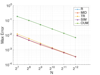
(c)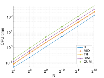 (d)
(d)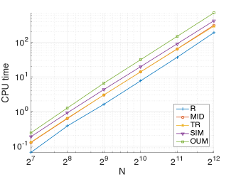
(e)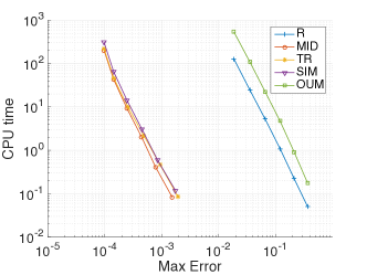 (f)
(f)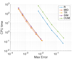
(a)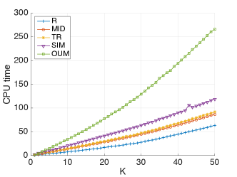 (b)
(b)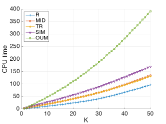
3.3 Effects of the hierarchical update strategy on numerical errors in OLIM-R
The one-point update and the triangle update in OLIM-R and the OUM are equivalent. Therefore, if the CPU-saving hierarchical update strategy would not be implemented in OLIM-R, the numerical errors produced by these methods would coincide (in the exact arithmetics). However, the hierarchical update combined with numerical errors might lead to non-identical numerical solutions by the OUM and OLIM-R. Figs. 6(a) and (b) show that the maximal errors in these two methods are very close (the curves visually coincide). More detailed data for the maximal and RMS errors and CPU times in the OUM and OLIM-R are displayed in Tables 2 and 3 for SDEs (24) and (27) respectively. They indicate that the hierarchical update, in some cases, might increase the numerical error, but this increase is negligible. On the other hand, the CPU times in OLIM-R are approximately 4 times smaller.
| Method, , | Max Error | RMS error | CPU time, seconds |
|---|---|---|---|
| OUM, | |||
| 1.7669e-01 | 1.0440e-01 | 2.05 | |
| 1.2133e-01 | 7.9878e-02 | 3.69 | |
| 1.2058e-01 | 7.9659e-02 | 5.60 | |
| OLIM-R, | |||
| 1.8368e-01 | 1.0706e-01 | 0.55 | |
| 1.2133e-01 | 7.9878e-02 | 0.88 | |
| 1.2058e-01 | 7.9659e-02 | 1.26 | |
| OUM, | |||
| 8.3905e-02 | 5.2161e-02 | 11.63 | |
| 6.6225e-02 | 4.4102e-02 | 19.15 | |
| 6.5912e-02 | 4.3992e-02 | 26.29 | |
| OLIM-R, | |||
| 8.4836e-02 | 5.2346e-02 | 3.02 | |
| 6.6225e-02 | 4.4102e-02 | 4.56 | |
| 6.5912e-02 | 4.3992e-02 | 6.06 | |
| OUM, | |||
| 4.1289e-02 | 2.6584e-02 | 62.80 | |
| 3.5510e-02 | 2.3803e-02 | 94.16 | |
| 3.5350e-02 | 2.3743e-02 | 127.43 | |
| OLIM-R, | |||
| 4.1529e-02 | 2.6609e-02 | 15.04 | |
| 3.5510e-02 | 2.3803e-02 | 21.55 | |
| 3.5350e-02 | 2.3743e-02 | 28.60 | |
| OUM, | |||
| 2.6959e-02 | 1.6629e-02 | 263.71 | |
| 1.9089e-02 | 1.2776e-02 | 397.53 | |
| 1.8656e-02 | 1.2599e-02 | 535.13 | |
| OLIM-R, | |||
| 2.7204e-02 | 1.6702e-02 | 66.76 | |
| 1.9051e-02 | 1.2769e-02 | 96.03 | |
| 1.8656e-02 | 1.2599e-02 | 127.22 |
| Method, , | Max Error | RMS error | CPU time, seconds |
|---|---|---|---|
| OUM, | |||
| 5.1079e-02 | 2.1963e-02 | 2.71 | |
| 5.0563e-02 | 2.1874e-02 | 5.05 | |
| 5.0563e-02 | 2.2332e-02 | 7.71 | |
| OLIM-R, | |||
| 5.1925e-02 | 2.2371e-02 | 0.81 | |
| 5.0850e-02 | 2.1940e-02 | 1.29 | |
| 5.0845e-02 | 2.2371e-02 | 1.83 | |
| OUM, | |||
| 2.5930e-02 | 1.1245e-02 | 20.50 | |
| 2.5890e-02 | 1.1447e-02 | 36.65 | |
| 2.5890e-02 | 1.1696e-02 | 53.57 | |
| OLIM-R, | |||
| 2.6182e-02 | 1.1283e-02 | 5.36 | |
| 2.6031e-02 | 1.1454e-02 | 8.71 | |
| 2.6025e-02 | 1.1692e-02 | 12.21 | |
| OUM, | |||
| 1.3478e-02 | 5.8271e-03 | 83.24 | |
| 1.3204e-02 | 5.8695e-03 | 193.00 | |
| 1.3189e-02 | 6.0301e-03 | 311.84 | |
| 1.3190e-02 | 6.1811e-03 | 443.35 | |
| OLIM-R, | |||
| 1.3656e-02 | 5.8558e-03 | 22.78 | |
| 1.3215e-02 | 5.8607e-03 | 46.23 | |
| 1.3200e-02 | 6.0178e-03 | 72.81 | |
| 1.3201e-02 | 6.1618e-03 | 103.35 | |
| OUM, | |||
| 7.2210e-03 | 3.0923e-03 | 341.70 | |
| 6.6921e-03 | 2.9666e-03 | 791.00 | |
| 6.6527e-03 | 3.0332e-03 | 1276.04 | |
| 6.6506e-03 | 3.0975e-03 | 1811.45 | |
| OLIM-R, | |||
| 7.3480e-03 | 3.1267e-03 | 101.85 | |
| 6.7011e-03 | 2.9587e-03 | 210.50 | |
| 6.6555e-03 | 3.0230e-03 | 326.48 | |
| 6.6536e-03 | 3.0859e-03 | 463.64 |
3.4 Comparison of OLIM-MID, OLIM-TR, and OLIM-SIM to each other
The comparison of OLIM-MID, OLIM-TR, and OLIM-SIM is conducted using , i.e., according to the Rule-of-Thumb for OLIM-MID, OLIM-TR, and OLIM-SIM. Fig. 8 shows that all these three methods are quite close in accuracy. Fig. 7 indicates that OLIM-SIM is somewhat slower than OLIM-MID and OLIM-TR. The least squares fits to the formulas for the maximum absolute errors and the RSM errors as functions of () are given in Table 4. OLIM-MID gives the best results on SDE (24) while OLIM-TR and OLIM-SIM challenge it on SDE (27) for rough meshes.
We favor OLIM-MID method. For fine meshes, it has the best balance between the accuracy and the CPU time among all methods considered in this work.
| Method | Max Error | RMS Error | Max Error | RMS Error |
|---|---|---|---|---|
| OLIM-MID | ||||
| OLIM-TR | ||||
| OLIM-SIM |
(a)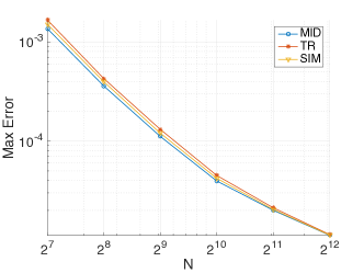 (b)
(b)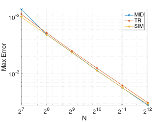
(c)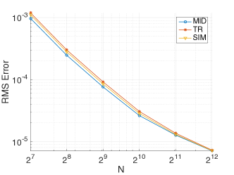 (d)
(d)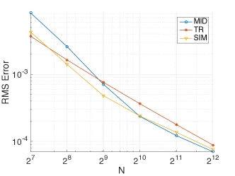
(e)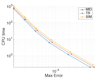 (f)
(f)
The error plots for each of the methods for SDEs (24) and (27) for the meshes and (corresponds to the Rule-of-Thumb) are shown in Fig. 9. We will return to the discussion on the error distributions in Section 4 below. Now we just note that these error plots are consistent with the results of Section 4. As we will show, the midpoint quadrature rule tends to underestimate the line integral, the trapezoid rule tends to exaggerate it, and the Simpson rule can make errors of either sign.
(a)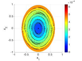 (b)
(b)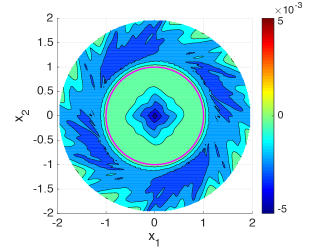
(c)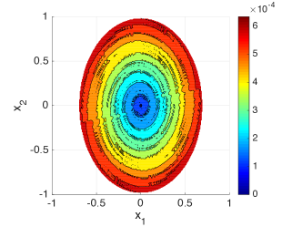 (d)
(d)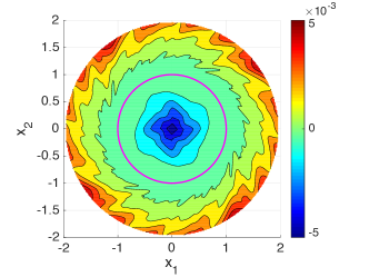
(e)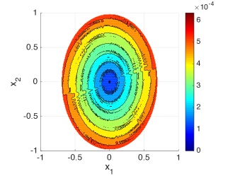 (f)
(f)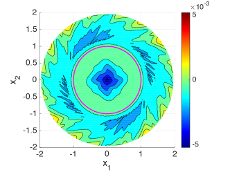
4 Origin of errors in the OLIMs
In this section, we discuss various factors which contribute to the error of the numerical solution by the OLIMs.
4.1 Errors of quadrature rules
In this Section, we discuss quadrature rule errors applied to the integral along a straight line segment connecting the points and
| (32) |
where
Let be the vector field at point . Assuming that is sufficiently small, we approximate by its Taylor expansion around :
where
Then the integral in Eq. (32) becomes
| (33) |
Approximating it using the quadrature rule with the error , we obtain
| (34) |
The errors of the right-hand, midpoint and trapezoid quadrature rules involve , , and (see e.g. [4]). For given by Eq. (33), one can easily evaluate these derivatives at . The resulting error estimates for the line integrals are
| (35) | ||||
| (36) | ||||
| (37) |
where , , and denote the right-hand, the midpoint, and the trapezoid basic quadrature rules respectively, and
| (38) | ||||
| (39) |
Eqs. (35) and (38) show that the integration error in OLIM-R is and can be of either sign. Eqs. (36) and (37) indicate that the integration errors in OLIM-MID and OLIM-TR are . The first term of (Eq. (39)) is due to the linear part of . It is nonnegative due to the Schwarz inequality. The second term of is due to the nonlinearity of . It can have an arbitrary sign. Therefore, the contribution to the error due to the linear part of is nonpositive for the midpoint rule, and nonnegative for the trapezoid rule. This is consistent with the error plots in Fig. 9(a) and (c) for the linear SDE.
Simpson’s quadrature rule has an error :
| (40) |
It is easy to calculate the contribution to due to the linear part of :
| (41) |
It can have an arbitrary sign. It is clear that the integration error in OLIM-SIM is small, and the total error of the numerical solution by OLIM-SIM, which is comparable to those by OLIM-MID and OLIM-TR (see Sec. 3.4), is due to the other factors discussed in Sections 4.3 and 4.2.
(a)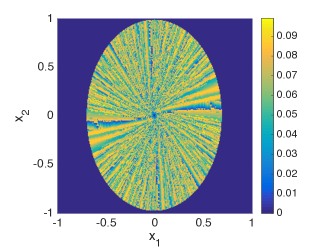 (b)
(b)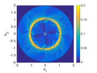
The lengths in Eqs. (35)-(37) and (40) can be recorded while the numerical solution is computed. For each mesh point we define the update length as the distance
for the one-point update, and
for the triangle update, where is the solution of the corresponding minimization problem in Eq. (18). We update every time when the value of the quasi-potential at is updated. The update lengths in the numerical solutions by OLIM-MID on mesh with for SDEs (24) and (27) are shown in Fig. 10 (a) and (b) respectively. The OLIMs are designed so that the update length can be at most which is and for the cases in Figs. 10 (a) and (b) respectively. For SDE (24), the update length is close to its maximal value at a significant fraction of mesh points. For SDE (27), it is close to its maximum in the outer neighborhood of the unit circle from which the computation starts. For the other OLIMs, the update lengths are similar. Therefore, the reduction of the integration error over rather long line segments by the use of second and higher order quadrature rules significantly improves the accuracy. This is exactly what we observe in Figs. 5 and 6.
4.2 Errors due to the curvatures of the level sets of the quasi-potential and MAPs
(a)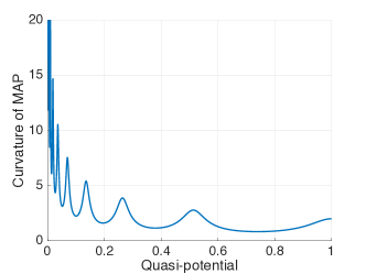 (b)
(b)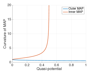
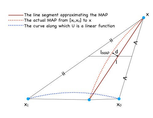
The OLIMs involve two contributions to their numerical errors due to the approximations of curved segments with straight line segments (Fig. 11). First, in both, the one-point and the triangle updates, curved segments of MAPs of lengths at most and respectively are approximated by straight line segments. Second, in the triangle update, curved segments of length at most along which the quasi-potential changes linearly, are approximated by straight line segments.
Let be the length of the line segment in the one-point update or in the triangle update approximating the MAP segment. Suppose that there is a MAP connecting the endpoints of this line segment, and its curvature is . Assume that is small and is constant. Then the length of the MAP segment is
| (42) |
OLIM-MID and OLIM-SIM involve the evaluation of at the midpoint of the line segment. The midpoint of the MAP segment is at distance from it:
| (43) |
The norm of the difference of evaluated at these two midpoints is proportional to . The curvature of MAPs can blow up near the equilibria of . As an example, the graphs of the curvature of the MAPs versus the quasi-potential along them for SDEs (24) and (27) are plotted in Fig. 12.
The bases of the triangles in the triangle update are at most of length . In the triangle update, the quasi-potential along the line segment is assumed to change linearly, while the actual curve along which the quasi-potential changes linearly, is not a straight line in general. For example, if , such a curve is the corresponding level set. For SDEs (24) and (27), such level sets are ellipses and circles respectively. Let be the curvature of the curve connecting and along which the quasi-potential is a linear function. Then the length of the segment of MAP connecting the point to be updated with this curve is shorter (as in Fig. 11) or longer than in Eq. (42) by at most
| (44) |
In summary, the local error of the triangle update due to approximating curved segments with line segments is bounded by
| (45) |
where is the Jacobian matrix of . Eq. (45) explains relatively large numerical errors near the origin by OLIM-MID, OLIM-TR, and OLIM-SIM applied to SDE (27) (see Fig. 9 (b), (d), and (f)).
The comparison of and the integration errors of the OLIMs (Eqs. (35), (36), (37), and (40)), combined with the results of our numerical tests in Section 3, show that the OLIMs are at most first order accurate regardless of the quadrature rule used. However, for a wide range of reasonable mesh sizes, OLIM-MID, OLIM-TR, and OLIM-SIM might appear to have superlinear convergence (see the least squares fits in Table 4) due to the change of the relative magnitudes of error terms of different orders. On the contrary, the OLIM-R exhibits sublinear convergence (see the least squares fits in Table 1).
4.3 Finite update radius
The direct application of the OUM developed in [17, 18] to the Hamilton-Jacobi PDE (3) for the quasi-potential would require an infinite update radius. The OUM adjusted for computing the quasi-potential [1] as well as the OLIMs set the update radius to where the update factor is a finite positive integer, and is the mesh step. The extra error due to the finite update radius may appear in the case where the angle between the normal to the level set of approximating the Accepted Front and the vector field at the point to be updated is close to (the angle in Fig. 3 (a, Top)). This extra error was quantified in [1] and shown not to exceed for sufficiently small .
To minimize this extra error, one might be tempted to use large values of the update factor . However, there is a trade-off. The quadrature errors are approximately proportional to where or 5 depending on the quadrature rule used (see Section 4.1), and the errors due to the curvature of MAPs and level sets of the quasi-potential are approximately . Hence, the optimal is the minimizer of the local error function of the form
where the coefficients , , and depend on the vector field and its derivatives, on the direction and the curvature of the MAPs, and on the curvature of the level sets of the quasi-potential. They change from one mesh point to another, and can have different orders of magnitude. Differentiating with respect to we get the following equation for the optimal :
In two simple cases, where or , the optimal is or respectively, i.e., or . In the general case, the dependence of the optimal on is more complicated, however, it is clear that must grow with but not faster that . Our numerical experiments suggest simple Rules-of-Thumb for choosing (see Section 3.1). It turns out that does not need to be very large.
5 Conclusion
We have introduced the family of Ordered Line Integral Methods (OLIMs) for computing the quasi-potential on a rectangular mesh. The update rules in OLIM-R, employing the right-hand rectangle quadrature rule, are equivalent to those in the OUM. OLIM-MID, OLIM-TR, and OLIM-SIM (employing the midpoint, the trapezoid, and Simpson’s quadrature rules) converge faster and admit errors two to three orders of magnitude smaller than OLIM-R and the OUM (See Fig. 5). Nevertheless, asymptotically, the OLIMs, like the OUM, are at most first order accurate due to the use of linear interpolation. While the use of second or higher order quadrature rules requires the use of a nonlinear solver and hence makes the triangle update more expensive than the one in the OUM, the proposed hierarchical update strategy for reducing the number of calls for the triangle update makes the OLIMs faster than the OUM. Due to this strategy, OLIM-R is about four times faster than the OUM. OLIM-MID and OLIM-TR are about 1.5 times faster than the OUM for the optimal ’s and about three times faster for (see Fig. 7). Our C codes OLIM_righthand.c, OLIM_midpoint.c, OLIM_trapezoid.c and OLIM_simpson.c implementing the corresponding OLIMs are available on M. Cameron’s website [2].
We have investigated the dependence of the error upon the update factor and concluded that, while large nearly eliminates the error in the direction of the MAP due to insufficient update radius in the case of a slowly changing vector field , it increases the integration error and the error due to the curvature of the MAP. Based on our study of the relationship between the numerical error and the update factor , we have proposed Rules-of-Thumb for choosing .
Our comparison of the OLIMs with second or higher order quadrature rules shows that the best one of them in terms of the balance between the accuracy and the CPU time is achieved by OLIM-MID.
The present work is focused on the 2D case with isotropic diffusion. The OLIMs can be extended to the case with anisotropic diffusion and to 3D. We will report these developments in the future.
Acknowledgements
We thank Professor A. Vladimirsky for a valuable discussion. This work was supported in part by the NSF grant DMS1554907.
Appendix A. The Freidlin-Wentzell action vs the Geometric action
The Freidlin-Wentzell action functional for SDE (1) is defined on the set of absolutely continuous paths by [6]
| (A-1) |
The original definition of the quasi-potential [6] with respect to a compact set (an attractor of ) at a point is
| (A-2) |
The minimization with respect to the travel-time can be performed analytically [6, 8, 9] resulting at the geometric action . Let be a fixed absolutely continuous path . Expanding in Eq. (A-1) and using the inequality for all nonnegative real numbers and , we get:
| (A-3) | ||||
The inequality in Eq. (A-3) becomes an equality if and only if . Let be the path obtained from by a reparametrization such that . Then
| (A-4) |
Note that can be infinite. The integral in right-hand side of Eq. (A-5) is invariant with respect to the parametrization of the path . Hence, we can pick the most convenient one, for example, the arclength parametrization, and denote the reparametrized path by . Hence,
| (A-5) |
where is the length of the paths and (corresponding to the same curve). For computation of the quasi-potential, it is more convenient to deal with the geometric action than with the Freidlin-Wentzell action .
Appendix B. The triangle updates for the OLIMs
OLIM-R
OLIM-R performs the triangle update by solving the following minimization problem
| (B-1) | |||
Taking the derivative of the function to be minimized
with respect to and setting it to zero, we obtain the following equation for :
| (B-2) |
Regrouping terms and taking squares we obtain the following quadratic equation for :
| (B-3) | ||||
| (B-4) | ||||
| (B-5) | ||||
| (B-6) |
We solve Eq. (B-3), select its root , if any, on the interval , and verify that it is also the root of Eq. (B-2). In the case of success, the triangle update returns
Otherwise, it returns .
OLIM-MID
OLIM-MID performs the triangle update by solving the following minimization problem
| (B-7) | ||||
Taking the derivative of
with respect to and setting it to zero, we obtain the following equation for :
| (B-8) |
The hybrid nonlinear solver [20, 19] is used for finding a root of Eq. (B-8) in the interval . In the case of success, the triangle update returns
Otherwise, it returns .
OLIM-TR
OLIM-TR performs the triangle update by solving the following minimization problem
| (B-9) | ||||
| where | ||||
Taking the derivative of
with respect to and setting it to zero we obtain the following equation for :
| (B-10) |
The hybrid nonlinear solver [20, 19] is used for finding a root of Eq. (B-10) in the interval . In the case of success, the triangle update returns
Otherwise, it returns .
OLIM-SIM
OLIM-SIM performs the triangle update by solving the following minimization problem
| (B-11) | ||||
| where | ||||
Taking the derivative of
with respect to and setting it to zero, we obtain the following equation for :
| (B-12) | |||
The hybrid nonlinear solver [20, 19] is used for finding a root of Eq. (B-12) in the interval . In the case of success, the triangle update returns
Otherwise, it returns .
Appendix C. Proof of Theorem 1
Proof.
Without the loss of generality we assume that is the origin.
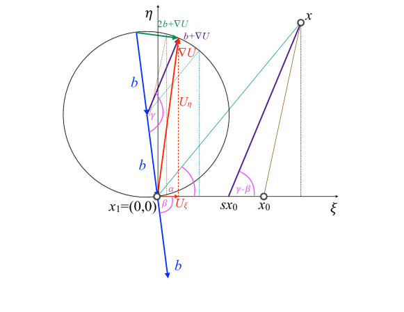
Step 1. Show that is a solution of Eq. (20) if and only if where (see Fig. 13) () is the angle between the vectors and , , and is a solution of
| (C-1) |
which is Eq. (3) written in the -coordinates at the point .
First observe that both Eqs. (20) and (22) are invariant with respect to translations. Therefore, we shift to the origin as shown in Fig. 13 without changing their solutions.
Second, Eq. (20) is invariant with respect to orthogonal transformations. Indeed, the multiplication of and by an orthogonal matrix converts Eq. (19) to
| (C-2) |
Hence the matrix in Eq. (20) changes to and becomes leading to the equation
| (C-3) |
which is equivalent to Eq. (20). Hence, we apply an orthogonal transformation to map the original coordinate system onto the system in which lies on the positive -semiaxis and the -coordinate of is positive:
where () is the angle between vectors and as shown in Fig. 13.
Finally, if is a solution of Eq. (20) then
Hence, if is the solution of Eq. (20), then is exactly which shows that it is independent of . Hence Eq. (20) can be rewritten as an equation Eq. (C-1) for .
Step 2. Find geometric conditions guaranteeing the existence of solution(s) of Eq. (C-1) satisfying the consistency check and determine the selection rule if it has two solutions.
Eq. (3) implies that is orthogonal to . Therefore, the locus of the vectors satisfying Eq. (3) is the circle [1] shown in Fig. 13. This circle passes through the origin and has center at the end of the vector originating from the origin. Since , Eq. (3) has a solution if and only if the line normal to the -axis and passing through the point (the red dashed line in Fig. 13) intersects the circle. The MAP is collinear to the vector [1]. The consistency condition requires that the MAP passing through the point crosses the interval . This means that the angle between the vector and the positive -semiaxis should be not less than the angle between the vector and the positive -semiaxis, and not greater than the angle between the vector and the positive -semiaxis. Drawing rays parallel to and from the center of the circle and then dropping normals from their intersections with the circle to the -axis as shown in Fig. 13, we obtain the interval on the -axis where should belong in order to make the solution of Eq. (C-1) satisfy the consistency condition. This interval bounded by the endpoints of the thin brown and green-blue dashed lines in Fig. 13. Note that the consistency condition can be satisfied only by the larger root of Eq. (C-1), i.e., we should select the root
| (C-4) |
Step 3. Find the solution of the minimization problem (22) and show that, if the minimizer then it coincides with , where and is given by Eq. (C-4).
Consider the function to be minimized in Eq. (22) rewritten for shifted to the origin:
| (C-5) |
where is the angle between the vectors and . The point , and hence the value of , is uniquely determined by the angle (Fig. 13):
| (C-6) |
Moreover, since is a monotone function on the interval , there is a one-to-one correspondence between and . Therefore, the function , , where
| (C-7) |
If is a minimum of , then there is a unique minimum of .
Let us minimize . Its derivative is given by:
Setting it to zero, cancelling the positive constant , regrouping the terms, and applying trigonometric formulas, we obtain the following equation for :
| (C-8) |
Hence, the optimal angle satisfies:
| (C-9) |
Let us denote by the solution of Eq. (C-9) lying in the interval . To check whether is a maximizer or a minimizer, we evaluate the second derivative of at and find:
| (C-10) |
as the angle by construction. Hence the optimal is the minimizer of . Next, we recall Eq. (3): . Adding to both sides, we obtain . Then Eq. (C-9) and the equality imply
| (C-11) |
Therefore,
| (C-12) |
On the other hand, from Eq. (C-9) we obtain:
| (C-13) |
Plugging Eq. (C-13) into Eq. (C-12) we get
| (C-14) |
which coincides with Eq. (C-4).
Finally, the solution of the minimization problem (22)
is achieved either at if , or at the endpoints or . Hence, if , then the solution of the minimization problem (22) coincides with the one of the finite difference scheme (20), and the latter meets the consistency conditions. Conversely, the solution of the finite difference scheme (20) satisfying the consistency conditions coincides with the one of the minimization problem (22), and the corresponding minimizer .
∎
References
- [1] M. K. Cameron, Finding the Quasipotential for Nongradient SDEs, Physica D: Nonlinear Phenomena, 241, pp. 1532-1550 (2012)
- [2] https://www.math.umd.edu/ mariakc/software-and-datasets.html
- [3] Z. Chen, M. Freidlin, Smoluchowski-Kramers approximation and exit problems, Stoch. Dyn. 5, 4, 569-585 (2005)
- [4] S. D. Conte and Carl de Boor, Elementary Numerical Analysis: an algorithmic approach, Third Edition, McGraw-Hill Book Company, 1980
- [5] M. G. Crandall, P. L. Lions, Viscosity solutions of Hamilton-Jacobi-Bellman equations, Trans. Amer. Math. Soc. 277, 1-43 (1983)
- [6] M. I. Freidlin and A. D. Wentzell, Random Perturbations of Dynamical Systems, 3rd ed, Springer-Verlag Berlin Heidelberg (2012)
- [7] T. Grafke, R. Grauer, and T. Schaefer, The instanton method and its numerical implementation in fluid mechanics, J. Phys. A: Math. Theor., 48, 33, 333001 (2015)
- [8] M. Heymann, E. Vanden-Eijnden, Pathways of maximum likelihood for rare events in non-equilibrium systems, application to nucleation in the presence of shear, Phys. Rev. Lett. 100, 14, 140601 (2007)
- [9] M. Heymann, E. Vanden-Eijnden, The geometric minimum action method: a least action principle on the space of curves, Comm. Pure Appl. Math. 61, 8, 1052-1117 (2008)
- [10] W.Hurewicz, Lectures on Ordinary Differential Equations, Dover Publications, New York (1990) (Originally, this book was published by the M.I.T. Press, Cambridge, Mass, in 1958).
- [11] H. Ishii, A simple direct proof of uniqueness for solutions of the Hamilton-Jacobi equations of eikonal type, Proc. Amer. Math. Soc. 100, 2, 247-251 (1987)
- [12] Cheng Lv, Xiaoguang Li, Fangting Li, Tiejun Li, Constructing the Energy Landscape for Genetic Switching System Driven by Intrinsic Noise, PLOS ONE, 9, 2, e88167 (2014)
- [13] R.S. Maier and D.L. Stein, A scaling theory of bifurcations in the symmetric weak- noise escape problem, J. Stat. Phys. 83, 3-4, 291357 (1996)
- [14] B. C. Nolting and K. C. Abbot, Balls, cups, and quasi-potentials: quantifying stability in stochastic systems, Ecology, 97, 4, 850-864 (2016)
- [15] B. Nolting, C. Moore, C. Stieha, M. Cameron, K. Abbott, QPot: An R package for stochastic differential equation quasi-potential analysis, R Journal 8, 2, 19-38 (2016)
- [16] https://cran.r-project.org/web/packages/QPot/index.html
- [17] J.A. Sethian and A. Vladimirsky. Ordered upwind methods for static Hamilton-Jacobi equations. Proc. Natl. Acad. Sci. USA 98, 20, 11069-11074 (2001)
- [18] J.A. Sethian and A. Vladimirsky. Ordered Upwind Methods for Static Hamilton-Jacobi Equations: Theory and Algorithms. SIAM J. on Numerical Analysis 41 1, 325-363 (2003)
- [19] J. W. Stewart, Afternotes on Numerical Analysis, SIAM, Philadelphia (1996)
- [20] J. Wilkinson, Two Algorithms Based on Successive Linear Interpolation, Computer Science, Stanford University, Technical Report CS-60 (1967)
- [21] Xiang Zhou, Weiqing Ren, and Weinan E, Adaptive minimum action method for the study of rare events, The Journal of Chemical Physics 128, 104111 (2008)
- [22] Xiang Zhou and Weinan E, Study of noise-induced transitions in the Lorenz system using the Minimum Action Method, Commun. Math. Sci. 8, 2, 341-355 (2010)