Domains in metric measure spaces with boundary of positive mean curvature, and the Dirichlet problem for functions of least gradient

Abstract

We study the geometry of domains in complete metric measure spaces equipped with a doubling measure supporting a $1$-Poincaré inequality. We propose a notion of domain with boundary of positive mean curvature and prove that, for such domains, there is always a solution to the Dirichlet problem for least gradients with continuous boundary data. Here least gradient is defined as minimizing total variation (in the sense of BV functions) and boundary conditions are satisfied in the sense that the boundary trace of the solution exists and agrees with the given boundary data. This extends the result of Sternberg, Williams and Ziemer [27] to the non-smooth setting. Via counterexamples we also show that uniqueness of solutions and existence of continuous solutions can fail, even in the weighted Euclidean setting with Lipschitz weights.

1 Introduction

The work of Giusti [12] showed a close connection between the curvature of the boundary of a Euclidean domain $\Omega\subset{\mathbb{R}}^{n}$ and the existence of a solution to the Dirichlet problem related to the Plateau problem

$$\operatorname{div}(\nabla u(1+|\nabla u|^{2})^{−1/2})=H(x,u(x))\quad\text{ for }{\mathscr{L}}^{n}\text{-a.e.\@ }x\in\Omega,$$

with the graph of $u$ a minimal surface (under the constraint that it has prescribed mean curvature) in ${\mathbb{R}}^{n+1}$. The work of Barozzi and Massari [5] studied a related obstacle problem for BV energy minimizers, where the obstacle is required to have a certain curvature condition analogous to that of [27]. While the conditions in [27] only considered domains whose boundary is of non-negative (or positive) mean curvature, the paper [5] imposed a more general mean curvature condition on the obstacle $M$, namely, that if $g\in L^{1}_{{\mathrm{loc}}}(\Omega)$ and $M\subset\Omega$, then $M$ is of mean curvature at most $g$ if

$$P(M,\Omega^{\prime})\leq P(F,\Omega^{\prime})+\int_{M\setminus F}g$$

whenever $\Omega^{\prime}\Subset\Omega$ and $F\bigtriangleup M\Subset\Omega^{\prime}$. The notion of non-negative mean curvature of $\partial\Omega$ (for $\Omega$ whose boundary need not be smooth), as given in [27] is not quite this condition, but is similar. Following this, the work of [27] showed that the Dirichlet problem related to the least gradient problem

$$\text{div}\frac{\nabla u}{|\nabla u|}=0\text{ in }\Omega,\quad Tu=f\text{ on }\partial\Omega,$$

has a solution if and only if $\partial\Omega$ has non-negative mean curvature (with respect to the domain $\Omega$) and $\partial\Omega$ is nowhere locally area-minimizing. Here $Tu$ is the trace of $u$ to $\partial\Omega$ (see the next section for its definition and discussion regarding its existence). More general notions of Dirichlet problem such as minimizing the energy integral

$$I(u)=\|Du\|(\overline{\Omega})$$

and the energy functional

$$J(u)=\|Du\|(\Omega)+\int_{\partial\Omega}|Tu-f|\,d{\mathcal{H}}$$ (1.1)

over all BV functions $u$ on ${\mathbb{R}}^{n}$ (with $u=f$ on ${\mathbb{R}}^{n}\setminus\Omega$ for the energy $I$) were studied for more general Euclidean domains, for example, in [8], see also the discussions in [13, 4, 27, 22]. Should we obtain a BV energy minimizer on $\Omega$ with the correct trace $f$ on $\partial\Omega$, then this solution also minimizes $I$ and $J$. Until the work of Sternberg, Williams, and Ziemer [27], not much consideration was given to how the trace of the minimizers fit in with the boundary data.

The recent development of first order analysis in the metric setting (see [17]) led to the extension of the theory of BV functions and functions of least gradient in the metric setting, see [23, 1, 2, 3, 18, 15] for a sample. The papers [15, 19] studied minimizers of the energy functionals $I$ and $J$ in the metric setting. The goal of the present paper is to study existence of the strongest possible solutions to the Dirichlet problem in the metric setting, namely that the solution obtains the correct prescribed trace value on the boundary of the domain of interest.

In addition to Euclidean domains as mentioned above, curvature conditions for the boundary of the domain also show up in the Heisenberg setting. Extending some of the results regarding the Plateau problem from the Euclidean space (see for example [11, 13]) to the Heisenberg setting, the recent paper [24] studied a related minimization problem in the Heisenberg setting, and there too it seems curvature of the boundary plays a role. More specifically, in [24] it is shown that if $\Omega\subset{\mathbb{R}}^{2n}$ is a bounded Lipschitz domain and $\varphi$ is a Lipschitz function on $\partial\Omega$ that is affine on the parts of the boundary where the domain is not positively curved, then there is a function $u$ on $\Omega$ such that the subgraph of $u$ in ${\mathbb{R}}^{2n}\times{\mathbb{R}}$, equipped with the Heisenberg metric, is of minimal boundary surface with the trace of $u$ on $\partial\Omega$ equal to $\varphi$, and furthermore, $u$ is Lipschitz continuous on $\Omega$. The work of [24] therefore is also concerned with the minimal graph problem rather than the least gradient problem. Any discussion of the Dirichlet problem for least gradient functions on domains in the Heisenberg group itself should be governed by curvature of the boundary of the domain as well.

We propose an analog (Definition 4.1) of the notion of positive mean curvature from the weak formulation of [27] to the metric setting where the measure is doubling and supports a $1$-Poincaré inequality. The main theorem of this paper, Theorem 4.11, will demonstrate the existence of such a strong solution to the least gradient problem for (globally) continuous BV boundary data provided the boundary of the domain is of positive mean curvature in the sense considered here. We will also show in the last section of this paper that outside of the Euclidean setting, continuity (inside the domain) of the solution and uniqueness of the solution can fail; indeed, the examples we provide can easily be modified to be a domain in a Riemannian manifold. We point out that our definition of positive mean curvature of the boundary is somewhat different from that of [27], see Remark 4.2 below.

The focus of [27] was Lipschitz boundary data; for such data, the authors prove that the solutions obtained are also Lipschitz (up to the boundary). The examples we provide here show that even with Lipschitz boundary data, Lipschitz continuity of the solution is not guaranteed in the general setting (not even in the Riemannian setting). Therefore, we broaden our scope to the wider class of all globally continuous BV functions as boundary data. We also show that if $\Omega$ satisfies some additional conditions, then it suffices to know that the boundary datum $f$ is merely a continuous function on the boundary $\partial\Omega$, see Section 5.

The primary tool developed in the present paper, “stacking pancakes with minimal boundary surface”, uses the idea that superlevel sets of functions of least gradient are of minimal boundary surface (in the sense of [18]). In the Euclidean setting, this was first proven by Bombieri, De Giorgi, and Giusti in [7], and was used in that spirit in the work [27], which inspired our work presented here. In the metric setting this minimality of the layers, or superlevel sets, was proven in [15]. While this method of “stacking pancakes” is similar to the one in [27], the tools available to us in our setting are very limited. In particular, we do not have the smoothness properties and tangent cones for boundaries of sets of minimal boundary surfaces, and hence the construction of “pancakes” (superlevel sets) given in [27] is not permitted to us. Furthermore, in the Euclidean setting, it is shown in [27] that if two sets $E_{1},E_{2}$ of minimal boundary surface such that $E_{1}\subset E_{2}$ have intersecting boundaries, then the two boundaries coincide in a relatively open set, and hence it holds that $E_{1}=E_{2}$. This property is used to show that the function constructed from the “stack of pancakes” is necessarily continuous, and thus issues of measurability of the constructed function does not arise in the Euclidean setting of [27]. In the metric setting this property fails (see the examples constructed in the final section of this paper). Consequently we had to modify our construction of the solution function from the “stack of pancakes” by considering a countable sub-stack of pancakes.

2 Notations and definitions in metric setting

We will assume throughout the paper that $(X,d,\mu)$ is a complete metric space endowed with a doubling measure $\mu$ that satisfies a $1$-Poincaré inequality defined below. We say that the measure $\mu$ is doubling on $X$ if there is a constant $C_{D}\geq 1$ such that

$$0<\mu(B(x,2r))\leq C_{D}\,\mu(B(x,r))<\infty$$

whenever $x\in X$ and $r>0$. Here $B(x,r)$ denotes the open ball with center $x$ and radius $r$. Given measurable sets $E,F\subset X$, the symbol $E\sqsubset F$ will denote that $\mu(E\setminus F)=0$ or, in other words, $\chi_{E}\leq\chi_{F}$ $\mu$-a.e.

A complete metric space with a doubling measure is proper, that is, closed and bounded sets are compact. Since $X$ is proper, given an open set $\Omega\subset X$ we define $L^{1}_{{\mathrm{loc}}}(\Omega)$ to be the space of functions that are in $L^{1}(\Omega^{\prime})$ for every $\Omega^{\prime}\Subset\Omega$, that is, when the closure of $\Omega^{\prime}$ is a compact subset of $\Omega$. Other local spaces of functions are defined analogously.

Given a function $u:X\to\overline{{\mathbb{R}}}$, we say that a non-negative Borel-measurable function $g$ is an upper gradient of $u$ if

$$|u(y)-u(x)|\leq\int_{\gamma}g\,ds$$ (2.1)

whenever $\gamma$ is a non-constant compact rectifiable curve in $X$. The endpoints of $\gamma$ are denoted by $x$ and $y$ in the above inequality. The inequality should be interpreted to mean that $\int_{\gamma}g\,ds=\infty$ if at least one of $u(x)$, $u(y)$ is not finite.

We say that $X$ supports a $1$-Poincaré inequality if there are positive constants $C_{P}$, $\lambda$ such that

$$\fint_{B}|u-u_{B}|\,d\mu\leq C_{P}\,r\,\fint_{\lambda B}g\,d\mu$$

whenever $B=B(x,r)$ is a ball in $X$ and $g$ is an upper gradient of $u$. Here, $u_{B}:=\mu(B)^{-1}\int_{B}u\,d\mu=:\fint_{B}u\,d\mu$ is the average of $u$ on the ball $B$, and $\lambda B:=B(x,\lambda r)$.

Throughout this paper $C$ will denote a constant whose precise value is not of interest here and depends solely on $C_{D}$, $C_{P}$, $\lambda$, and perhaps on the domain $\Omega$. As $C$ stands for such a generic constant, its value could differ at each occurrence.

Let $\widetilde{N}^{1,1}(X)$ be the class of all $L^{1}$ functions on $X$ for which there exists an upper gradient in $L^{1}(X)$. For $u\in\widetilde{N}^{1,1}(X)$ we define

$$\|u\|_{\widetilde{N}^{1,1}(X)}=\|u\|_{L^{1}(X)}+\inf_{g}\|g\|_{L^{1}(X)},$$

where the infimum is taken over all upper gradients $g$ of $u$. Now, we define an equivalence relation in $\widetilde{N}^{1,1}(X)$ by $u\sim v$ if and only if $\|u-v\|_{\widetilde{N}^{1,1}(X)}=0$.

The Newtonian space $N^{1,1}(X)$ is defined as the quotient $\widetilde{N}^{1,1}(X)/\sim$ and it is equipped with the norm $\|u\|_{N^{1,1}(X)}=\|u\|_{\widetilde{N}^{1,1}(X)}.$ One can define analogously $N^{1,1}(\Omega)$ for an open set $\Omega\subset X$. For more on upper gradients and Newtonian spaces of functions on metric measure spaces, see [17].

For $u\in L^{1}_{{\mathrm{loc}}}(X)$ the total variation of $u$ is defined by

$$\|Du\|(X)=\inf\left\{\liminf_{i\to\infty}\int_{X}g_{u_{i}}\,d\mu:N^{1,1}_{{\mathrm{loc}}}(X)\ni u_{i}\to u\,\text{in }L^{1}_{{\mathrm{loc}}}(X)\right\},$$

where $g_{u_{i}}$ are upper gradients of $u_{i}$.

One can define analogously $\|Du\|(\Omega)$ for an open set $\Omega\subset X$. If $A\subset X$ is an arbitrary set we define

$$\|Du\|(A)=\inf\{\|Du\|(\Omega):\Omega\supset A,\Omega\subset X\,\text{open}\}.$$

A function $u\in L^{1}(X)$ is in $\mathrm{BV}(X)$ (of bounded variation) if $\|Du\|(X)<\infty$. For such $u$, $\|Du\|$ is a Radon measure on $X$, see [23, Theorem 3.4]. A $\mu$-measurable set $E\subset X$ is of finite perimeter if $\|D\chi_{E}\|(X)<\infty$. The perimeter of $E$ in $\Omega$ is

$$P(E,\Omega):=\|D\chi_{E}\|(\Omega).$$

BV energy on open sets is lower semicontinuous with respect to $L^{1}$-convergence, i.e., if $u_{k}\to u$ in $L^{1}_{\mathrm{loc}}(\Omega)$ as $k\to\infty$, where $\Omega\subset X$ is open, then

$$\|Du\|(\Omega)\leq\liminf_{k\to\infty}\|Du_{k}\|(\Omega)\,.$$ (2.2)

The coarea formula in the metric setting [23, Proposition 4.2] says that if $u\in L^{1}_{{\mathrm{loc}}}(\Omega)$ for an open set $\Omega$, then

$$\|Du\|(\Omega)=\int_{-\infty}^{\infty}P(\{u>t\},\Omega)\,dt,$$ (2.3)

If $\|Du\|(\Omega)<\infty$, the above holds with $\Omega$ replaced by any Borel set $A\subset\Omega$.

Given a set $E\subset X$, its Hausdorff measure of codimension 1 is defined by

$${\mathcal{H}}(E)=\lim_{r\to 0}\ \inf\left\{\sum_{i=1}^{\infty}\frac{\mu(B(x_{i},r_{i}))}{r_{i}}:E\subset\bigcup_{i=1}^{\infty}B(x_{i},r_{i}),r_{i}\leq r\right\}.$$

It is known from [1, Theorem 5.3] and [3, Theorem 4.6] that if $E\subset X$ is of finite perimeter, then for Borel sets $A\subset X$,

$$\frac{1}{C}{\mathcal{H}}(A\cap\partial_{m}E)\leq P(E,A)\leq C{\mathcal{H}}(A\cap\partial_{m}E),$$

where $\partial_{m}E$ is the measure-theoretic boundary of $E$, that is, the collection of all points $x\in X$ for which simultaneously

$$\limsup_{r\to 0^{+}}\frac{\mu(B(x,r)\cap E)}{\mu(B(x,r))}>0\quad\text{and}\quad\limsup_{r\to 0^{+}}\frac{\mu(B(x,r)\setminus E)}{\mu(B(x,r))}>0.$$

Given a bounded domain $\Omega\subset X$ and a function $u\in\mathrm{BV}(\Omega)$, we say that $u$ has a trace at a point $z\in\partial\Omega$ if there is a number $Tu(z)\in{\mathbb{R}}$ such that

$$\lim_{r\to 0^{+}}\fint_{B(z,r)\cap\Omega}|u(x)-Tu(z)|\,d\mu(x)=0.$$ (2.4)

We know from [20, Theorem 3.4, Theorem 5.5] and [21] that if $\Omega$ satisfies all of the following geometric conditions, then every function in $\mathrm{BV}(\Omega)$ has a trace $\mathcal{H}$-a.e. on $\partial\Omega$:

1. there is a constant $C\geq 1$ such that

   $$\mu(B(z,r)\cap\Omega)\geq\frac{\mu(B(z,r))}{C}$$

   whenever $z\in\overline{\Omega}$ and $0<r<2\operatorname{diam}(\Omega)$;

2. there is a constant $C\geq 1$ such that

   $$\frac{1}{C}\frac{\mu(B(z,r))}{r}\leq{\mathcal{H}}(B(z,r)\cap\partial\Omega)\leq C\,\frac{\mu(B(z,r))}{r}$$

   whenever $z\in\partial\Omega$ and $0<r<2\operatorname{diam}(\Omega)$;

3. $\Omega$ supports a $1$-Poincaré inequality.

Furthermore, if $\Omega$ satisfies all the above conditions, then the trace class of $\mathrm{BV}(\Omega)$ is $L^{1}(\partial\Omega,{\mathcal{H}})$.

Definition 2.5.

Let $\Omega\subset X$ be an open set, and let $u\in\mathrm{BV}_{{\mathrm{loc}}}(\Omega)$. We say that $u$ is of least gradient in $\Omega$ if

$$\|Du\|(V)\leq\|Dv\|(V)$$

whenever $v\in\mathrm{BV}(\Omega)$ with $\overline{\{x\in\Omega\,:\,u(x)\neq v(x)\}}\subset V\Subset\Omega$. A set $E\subset\Omega$ is of minimal boundary surface in $\Omega$, if $\chi_{E}$ is of least gradient in $\Omega$.

Definition 2.6.

Let $\Omega$ be a nonempty bounded domain in $X$ with $\mu(X\setminus\Omega)>0$, and let $f\in\mathrm{BV}_{{\mathrm{loc}}}(X)$. We say that $u\in\mathrm{BV}_{{\mathrm{loc}}}(X)$ is a weak solution to the Dirichlet problem for least gradients in $\Omega$ with boundary data $f$, or simply, weak solution to the Dirichlet problem with boundary data $f$, if $u=f$ on $X\setminus\Omega$ and

$$\|Du\|(\overline{\Omega})\leq\|Dv\|(\overline{\Omega})$$

whenever $v\in\mathrm{BV}(X)$ with $v=f$ on $X\setminus\Omega$.

Definition 2.7.

Let $\Omega$ be a nonempty domain in $X$ and $f:\partial\Omega\to{\mathbb{R}}$. We say that a function $u\in\mathrm{BV}(\Omega)$ is a solution to the Dirichlet problem for least gradients in $\Omega$ with boundary data $f$, or simply, solution to the Dirichlet problem with boundary data $f$, if $Tu=f$ $\mathcal{H}$-a.e. on $\partial\Omega$ and whenever $v\in\mathrm{BV}(\Omega)$ with $Tv=f$ $\mathcal{H}$-a.e. on $\partial\Omega$ we must have

$$\|Du\|(\Omega)\leq\|Dv\|(\Omega).$$

Note that solutions and weak solutions to Dirichlet problems on a domain $\Omega$ are necessarily of least gradient in $\Omega$.

Given a function $u$ on $X$ and $x\in X$, we define

$$u^{\vee}(x)=\mathop{\textup{ap-$\limsup_{y\to x}$}}u(y):=\inf\biggl{\{}t\in{\mathbb{R}}\colon\lim_{r\to 0^{+}}\frac{\mu(B(x,r)\cap\{u>t\})}{\mu(B(x,r))}=0\biggr{\}},$$

and

$$u^{\wedge}(x)=\mathop{\textup{ap-$\liminf_{y\to x}$}}u(y):=\sup\biggl{\{}t\in{\mathbb{R}}\colon\lim_{r\to 0^{+}}\frac{\mu(B(x,r)\cap\{u<t\})}{\mu(B(x,r))}=0\biggr{\}}.$$

Then, $u^{\vee}(x)=u^{\wedge}(x)$ for $\mu$-a.e. $x\in X$ by the Lebesgue differentiation theorem provided that $u\in L^{1}_{\mathrm{loc}}(X)$.

Points $x$ for which $u^{\vee}(x)=u^{\wedge}(x)$ are said to be points of approximate continuity of $u$. Let $S_{u}$ be the set of points $x$ at which $u$ is not approximately continuous. For $u\in\mathrm{BV}(X)$, the set $S_{u}$ is of $\sigma$-finite codimension 1 Hausdorff measure, see [3, Proposition 5.2]. If in addition $u=\chi_{E}$ for some $E\subset X$, then $S_{u}=\partial_{m}E$. By [3, Theorem 5.3], the Radon measure $\|Du\|$ associated with a function $u\in\mathrm{BV}(X)$ permits the following decomposition:

$$d\|Du\|=g\,d\mu+d\|D^{j}u\|+d\|D^{c}u\|,$$ (2.8)

where $g\,d\mu$ with $g\in L^{1}(X)$ gives the part of $\|Du\|$ that is absolutely continuous with respect to the underlying measure $\mu$ on $X$, and $\|D^{j}u\|$ is the so-called jump-part of $u$. This latter measure lives inside $S_{u}$, and is absolutely continuous with respect to ${\mathcal{H}}\lfloor_{S_{u}}$. The third measure, $\|D^{c}u\|$, is called the Cantor part of $\|Du\|$, and does not charge sets of $\sigma$-finite codimension 1 Hausdorff measure. In the literature, the set $S_{u}$ is called the jump set of $u$, see [1, 2, 3].

It was shown in [15] that functions of least gradient, after a modification on a set of measure zero, are continuous everywhere outside their jump sets.

3 Preliminary results related to weak solutions

Throughout the rest of this paper, we will assume that $X$ is a complete metric space equipped with a doubling measure $\mu$ supporting a $1$-Poincaré inequality, and $\Omega\subset X$ is a nonempty bounded domain such that $\mu(X\setminus\Omega)>0$.

We will need the next lemma for functions of the form $f=\chi_{F}$ for sets $F\subset X$ of finite perimeter.

Lemma 3.1.

For every $f\in\mathrm{BV}_{\mathrm{loc}}(X)$ such that $\|Df\|(X)<\infty$ there is a function $u_{f}\in\mathrm{BV}_{\mathrm{loc}}(X)$ that is a weak solution to the Dirichlet problem in $\Omega$ with boundary data $f$.

Proof.

Let

$$I:=\inf\{\|Du\|(\overline{\Omega})\,:\,u\in\mathrm{BV}_{\mathrm{loc}}(X)\text{ and }u=f\text{ on }X\setminus\Omega\}.$$

Observe that $0\leq I\leq\|Df\|(\overline{\Omega})<\infty$. Let $\{u_{k}\}_{k=1}^{\infty}$ be a sequence of functions in $\mathrm{BV}_{\mathrm{loc}}(X)$ with $u_{k}=f$ on $X\setminus\Omega$ such that $\|Du_{k}\|(\overline{\Omega})\to I$ as $k\to\infty$. Let $B\subset X$ be an open ball that contains $\overline{\Omega}$. In particular, we can choose $B$ so that $\mu(B\setminus\Omega)>0$. Hence, the $1$-Poincaré inequality yields that

$$\int_{B}|u_{k}-f|\,d\mu\leq C_{B,\Omega}\|D(u_{k}-f)\|(\overline{\Omega}) \leq C_{B,\Omega}\bigl{(}\|Du_{k}\|(\overline{\Omega})+\|Df\|(\overline{\Omega})\bigr{)}$$

$$\leq 3C_{B,\Omega}\|Df\|(\overline{\Omega})$$

for sufficiently large $k$. Note that the above holds true without subtracting $(u_{k}-f)_{B}$ on the left-hand side because $u_{k}-f=0$ on $B\setminus\Omega$, while $\mu(B\setminus\Omega)$ is positive, see for example [18, Lemma 2.2]. Thus, the sequence $\{u_{k}-f\}_{k=1}^{\infty}$ is bounded in $\mathrm{BV}(B)$, and hence so is $\{u_{k}\}_{k=1}^{\infty}$. By the $1$-Poincaré inequality and the doubling property of $\mu$, the space $\mathrm{BV}(B)$ is compactly embedded in $L^{q}(B)$ for some $q>1$, see for example [14, 17] and [23, Theorem 3.7]. Therefore, there is a subsequence, also denoted $u_{k}$, that converges in $L^{q}(B)$ and pointwise $\mu$-a.e. in $B$ to a function $u_{0}\in\mathrm{BV}(B)$. By the fact that each $u_{k}=f$ on $X\setminus\Omega$, we have that $u_{0}=f$ on $B\setminus\Omega$, and that the extension of $u_{0}$ by $f$ to $X\setminus B$ yields a function in $\mathrm{BV}_{\mathrm{loc}}(X)$. We denote this extended function by $u_{f}$.

Finally, note by the lower semicontinuity of BV energy that

$$\|Du_{f}\|(\overline{\Omega})+\|Df\|(B\setminus\overline{\Omega})=\|Du_{f}\|(B)\leq\liminf_{k\to\infty}\|Du_{k}\|(B)=I+\|Df\|(B\setminus\overline{\Omega}),$$

that is, $\|Du_{f}\|(\overline{\Omega})\leq I$. Since $u_{f}=f$ on $X\setminus\Omega$ and $u_{f}\in\mathrm{BV}_{\mathrm{loc}}(X)$, it follows that $\|Du_{f}\|(\overline{\Omega})=I$. This completes the proof of the lemma. ∎

In the following lemma, we will see that the Dirichlet problem in $\Omega$ with boundary data $\chi_{F}$ for some set $F\subset X$ of finite perimeter has a weak solution given as a function $\chi_{E}$ for some set $E\subset\Omega\cup F$. Such a set $E$ will be called a weak solution set.

Lemma 3.2.

Let $F\subset X$ with $P(F,X)<\infty$. Then, there is a set $E\subset X$ with $P(E,X)<\infty$ such that $\chi_{E}$ is a weak solution to the Dirichlet problem in $\Omega$ with boundary data $\chi_{F}$.

Moreover, if $u_{\chi_{F}}$ is a weak solution to the Dirichlet problem with boundary data $\chi_{F}$, then we can pick any $t_{0}\in(0,1]$ and choose $E$ to be the set

$$E_{t_{0}}=\{x\in X\colon u_{\chi_{F}}(x)\geq t_{0}\}.$$

Proof.

By Lemma 3.1, there is a weak solution $u_{\chi_{F}}$. Note that $0\leq u_{\chi_{F}}\leq 1$ on $X$ by the maximum principle proven in [15, Theorem 5.1].

For $t\in(0,1]$, let

$$E_{t}=\{x\in X\,\colon\,u_{\chi_{F}}(x)\geq t\}.$$

We will first show that $\chi_{E_{t}}$ is a weak solution to the Dirichlet problem in $\Omega$ with boundary data $\chi_{F}$ for all $t\in(0,1]\setminus N$ for some negligible set $N$. We will prove that $N=\emptyset$ later.

The coarea formula (2.3), together with the fact that $P(F,X)<\infty$, gives that

$$\int_{0}^{1}P(E_{t},X)\,dt=\int_{-\infty}^{\infty}P(E_{t},X)\,dt=\|Du_{\chi_{F}}\|(X)\leq P(F,X)<\infty,$$

whence $P(E_{t},X)<\infty$ for ${\mathscr{L}}^{1}$-a.e. $t\in(0,1]$. Moreover, $\chi_{E_{t}}=\chi_{F}$ on $X\setminus\Omega$ for every $t\in(0,1]$. Since $u_{\chi_{F}}$ is a weak solution corresponding to the boundary data $\chi_{F}$, we have $\|Du_{\chi_{F}}\|(\overline{\Omega})\leq P(E_{t},\overline{\Omega})$ for every $t\in(0,1]$.

Let $N=\{t\in(0,1]\colon\|Du_{\chi_{F}}\|(\overline{\Omega})<P(E_{t},\overline{\Omega})\}$. Then by the coarea formula,

$$\|Du_{\chi_{F}}\|(\overline{\Omega})=\int_{0}^{1}P(E_{t},\overline{\Omega})\,dt =\int_{(0,1]\setminus N}\|Du_{\chi_{F}}\|(\overline{\Omega})\,dt+\int_{N}P(E_{t},\overline{\Omega})\,dt$$

$$=(1-{\mathscr{L}}^{1}(N))\|Du_{\chi_{F}}\|(\overline{\Omega})+\int_{N}P(E_{t},\overline{\Omega})\,dt.$$

Hence, ${\mathscr{L}}^{1}(N)\|Du_{\chi_{F}}\|(\overline{\Omega})=\int_{N}P(E_{t},\overline{\Omega})\,dt$, which can hold true only if ${\mathscr{L}}^{1}(N)=0$.

We have shown that $\chi_{E_{t}}=\chi_{F}$ on $X\setminus\Omega$ and $P(E_{t},\overline{\Omega})=\|Du_{\chi_{F}}\|(\overline{\Omega})$ for every $t\in(0,1]\setminus N$, where ${\mathscr{L}}^{1}(N)=0$. Therefore, for every $t\in(0,1]\setminus N$, the function $\chi_{E_{t}}$ is a weak solution with boundary data $\chi_{F}$, and we may choose $E$ to be the set $E_{t}$.

Let us now show that $N$ is in fact empty. Indeed, taking an arbitrary $t\in(0,1]$ and a sequence $t_{k}\in(0,1]\setminus N$ such that $t_{k}\nearrow t$, we obtain that $E_{t}=\bigcap_{k}E_{t_{k}}$ and hence $|\chi_{E_{t_{k}}}-\chi_{E_{t}}|\to 0$ in $L^{1}(X)$ as $k\to\infty$. The lower semicontinuity of the $\mathrm{BV}$ energy with respect to the $L^{1}$-convergence yields that

$$P(E_{t},\overline{\Omega})+P(F,X\setminus\overline{\Omega}) =P(E_{t},X)$$

$$\leq\liminf_{k\to\infty}P(E_{t_{k}},X)=\liminf_{k\to\infty}P(E_{t_{k}},\overline{\Omega})+P(F,X\setminus\overline{\Omega}).$$

Hence, $P(E_{t},\overline{\Omega})\leq\|Du_{\chi_{F}}\|(\overline{\Omega})$. In other words, $t\notin N$. ∎

Lemma 3.3.

Let $F_{1}\subset F_{2}\subset X$ be sets of finite perimeter in $X$. Suppose that $E_{1},E_{2}\subset X$ are chosen such that $\chi_{E_{1}}$ and $\chi_{E_{2}}$ are weak solutions to the Dirichlet problem in $\Omega$ with boundary data $\chi_{F_{1}}$ and $\chi_{F_{2}}$, respectively. Then, $\chi_{E_{1}\cap E_{2}}$ is a weak solution corresponding to $\chi_{F_{1}}$, while $\chi_{E_{1}\cup E_{2}}$ is a weak solution corresponding to $\chi_{F_{2}}$.

Proof.

From [23, Proposition 4.7(3)], together with the fact that the perimeter measure is a Borel regular outer measure, we know that

$$P(E_{1}\cap E_{2},\overline{\Omega})+P(E_{1}\cup E_{2},\overline{\Omega})\leq P(E_{1},\overline{\Omega})+P(E_{2},\overline{\Omega}).$$ (3.4)

If $P(E_{1}\cap E_{2},\overline{\Omega})>P(E_{1},\overline{\Omega})$, then we would have $P(E_{1}\cup E_{2},\overline{\Omega})<P(E_{2},\overline{\Omega})$. However, this would violate the minimality of $P(E_{2},\overline{\Omega})$ among all BV functions that equal $\chi_{F_{2}}$ outside $\Omega$ since $(E_{1}\cup E_{2})\setminus\Omega=(F_{1}\cup F_{2})\setminus\Omega=F_{2}\setminus\Omega$. Hence, $P(E_{1}\cap E_{2},\overline{\Omega})\leq P(E_{1},\overline{\Omega})$. Furthermore, ${(E_{1}\cap E_{2})\setminus\Omega}={(F_{1}\cap F_{2})\setminus\Omega}={F_{1}\setminus\Omega}$ and hence $\chi_{E_{1}\cap E_{2}}$ is a weak solution to the Dirichlet problem with boundary data $\chi_{F_{1}}$.

By a similar argument, we can rule out the inequality $P(E_{1}\cup E_{2},\overline{\Omega})>P(E_{2},\overline{\Omega})$ as it would violate the fact that $\chi_{E_{1}}$ is a weak solution for the boundary data $\chi_{F_{1}}$. Therefore, $P(E_{1}\cup E_{2},\overline{\Omega})\leq P(E_{2},\overline{\Omega})$ and we conclude that $\chi_{E_{1}\cup E_{2}}$ is a weak solution to the Dirichlet problem with boundary data $\chi_{F_{2}}$. ∎

Remark 3.5.

If $F_{1}\subset F_{2}$ are as in Lemma 3.3 and if $u_{\chi_{F_{1}}}$ and $u_{\chi_{F_{2}}}$ are weak solutions to the Dirichlet problem with boundary data $\chi_{F_{1}}$ and $\chi_{F_{2}}$, respectively, then one can use the coarea formula to prove that $\min\{u_{\chi_{F_{1}}},u_{\chi_{F_{2}}}\}$ and $\max\{u_{\chi_{F_{1}}},u_{\chi_{F_{2}}}\}$ are weak solutions corresponding to boundary data $\chi_{F_{1}}$ and $\chi_{F_{2}}$, respectively.

Definition 3.6.

A (weak) solution $\chi_{E}$ to the Dirichlet problem with boundary data $\chi_{F}$ is called a minimal (weak) solution to the said problem if every (weak) solution $\chi_{\widetilde{E}}$ corresponding to the data $\chi_{F}$ satisfies $E\sqsubset\widetilde{E}$, that is, $\mu(E\setminus\widetilde{E})=0$, or alternatively, $\chi_{E}\leq\chi_{\widetilde{E}}$ $\mu$-a.e. in $X$.

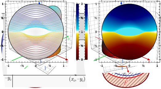
Figure 1: Two weak solutions $\chi_{E}$ to the Dirichlet problem in $\Omega$ with boundary data $\chi_{F}$, where $F$ is the (closed) region filled with light red color. The figure on the right shows the minimal weak solution. Each of the arcs of $\partial\Omega\cap\partial F$ and $\partial\Omega\setminus\partial F$ covers the angle of $\pi/2$. Note also that the restriction $\chi_{E}\bigr{|}_{\Omega}$ is a solution / the minimal solution.

Remark 3.7.

It follows from Lemma 3.2 that if $u_{\chi_{F}}$ is a weak solution and $\chi_{E}$ is the minimal weak solution to the Dirichlet problem with boundary data $\chi_{F}$, then $u_{\chi_{F}}\geq 1$ a.e. on $E$.

Proposition 3.8.

Let $F\subset X$ be a set of finite perimeter in $X$. Then, there exists a unique minimal weak solution $\chi_{E}$ to the Dirichlet problem in $\Omega$ with boundary data $\chi_{F}$.

Here, by uniqueness we mean that two minimal weak solutions agree $\mu$-almost everywhere in $X$.

Proof.

Let $\alpha=\inf_{E}\mu(E\cap\Omega)$, where the infimum is taken over all sets $E$ such that $\chi_{E}$ is a weak solution to the Dirichlet problem. Note that there is at least one such weak solution by Lemma 3.2. Moreover, $\alpha<\infty$ since $\mu(\Omega)<\infty$.

Let $\{E_{k}\}_{k=1}^{\infty}$ be a sequence of sets such that $\chi_{E_{k}}$ solves the Dirichlet problem and $\mu(E_{k}\cap\Omega)\to\alpha$ as $k\to\infty$. Let $\widetilde{E}_{1}=E_{1}$ and $\widetilde{E}_{k+1}=E_{k+1}\cap\widetilde{E}_{k}$, $k=1,2,\ldots$. By Lemma 3.3, each of the sets $\widetilde{E}_{k}$ gives a weak solution with the same boundary data $\chi_{F}$. Moreover, $\widetilde{E}_{k+1}\subset\widetilde{E}_{k}$ for all $k=1,2,\ldots$ and $\mu(\widetilde{E}_{k}\cap\Omega)\to\alpha$.

Let $E=\bigcap_{k}\widetilde{E}_{k}$. Then, $E\setminus\Omega=\bigcap_{k}(\widetilde{E}_{k}\setminus\Omega)=F\setminus\Omega$. As $X\setminus\overline{\Omega}$ is open and $\chi_{E}=\chi_{F}=\chi_{\widetilde{E}_{k}}$ in $X\setminus\overline{\Omega}$, we have

$$P(E,X\setminus\overline{\Omega})=P(F,X\setminus\overline{\Omega})=P(\widetilde{E}_{k},X\setminus\overline{\Omega})\quad\text{for every }k=1,2,\ldots.$$

Since $|\chi_{\widetilde{E}_{k}}-\chi_{E}|\to 0$ in $L^{1}(X)$, the lower semicontinuity of the BV energy (2.2) yields that $P(E,X)<\infty$ and then also

$$P(E,\overline{\Omega}) =P(E,X)-P(F,X\setminus\overline{\Omega})\leq\liminf_{k\to\infty}P(\widetilde{E}_{k},X)-P(F,X\setminus\overline{\Omega})$$

$$=\liminf_{k\to\infty}P(\widetilde{E}_{k},\overline{\Omega})=\inf\{\|Du\|(\overline{\Omega})\colon u=\chi_{F}\text{ in }X\setminus\Omega\}.$$

Thus, $\chi_{E}$ is a weak solution to the Dirichlet problem. If $E^{\prime}$ is another weak solution, then, by Lemma 3.3, so is $E\cap E^{\prime}$, and hence $\alpha\leq\mu(E\cap E^{\prime}\cap\Omega)\leq\mu(E\cap\Omega)=\alpha$. Therefore, $\mu(E\setminus E^{\prime})=0$, that is, $E$ is a minimal weak solution. The uniqueness now follows from the above argument, which yields that $\mu(E\bigtriangleup E^{\prime})=0$ whenever $E^{\prime}$ is another minimal weak solution. ∎

Lemma 3.9.

Let $F_{1}\sqsubset F_{2}\subset X$ be sets of finite perimeter in $X$. Then, the minimal weak solutions $\chi_{E_{1}}$ and $\chi_{E_{2}}$ to the Dirichlet problem in $\Omega$ with boundary data $\chi_{F_{1}}$ and $\chi_{F_{2}}$, respectively, satisfy $E_{1}\sqsubset E_{2}$.

Proof.

By replacing $F_{2}$ with $F_{2}\cup F_{1}$ if necessary (and in doing so, we only modify $F_{2}$ on a set of measure zero), we may assume that $F_{1}\subset F_{2}$. Let $E_{1}$ and $E_{2}$ be as in the statement of the lemma. By Lemma 3.3, $E_{1}\cap E_{2}$ gives a weak solution to the Dirichlet problem with boundary data $\chi_{F_{1}}$. Uniqueness of the minimal weak solutions implies that $\mu(E_{1}\setminus E_{2})=\mu(E_{1}\setminus(E_{1}\cap E_{2}))=0$. ∎

We will see in Proposition 4.9 that for domains with boundary of positive mean curvature, there is no need to distinguish between solutions and weak solutions for boundary data $\chi_{F}$. Hence, in such domains, there exists a unique minimal solution, and furthermore, the minimal solutions exhibit the same nesting property for nested boundary data as in Lemma 3.9.

It is, in fact, also possible to define a maximal (weak) solution $\chi_{E}$ to the Dirichlet problem in $\Omega$ with boundary data $\chi_{F}$ by requiring that $\mu(\widetilde{E}\setminus E)=0$ for every other (weak) solution $\chi_{\widetilde{E}}$ of the said problem. For instance, the set $E$ on the left in Figure 1 gives the maximal (weak) solution.

4 Domains in metric spaces with boundary of positive mean curvature

In this section we propose a notion of positive mean curvature of the boundary of a domain $\Omega$ in the metric measure space $X$, and study the Dirichlet problem for such domains. As explained in the introduction, solutions to Dirichlet problem in the sense of Definition 2.7 might not always exist. Given an open set $F\subset X$ that intersects $\partial\Omega$, let $u_{\chi_{F}}$ denote a generic weak solution to the Dirichlet problem with boundary data $\chi_{F}$. It is not necessarily true that $Tu_{\chi_{F}}=\chi_{F}$ ${\mathcal{H}}$-a.e. on $\partial\Omega$. The classic example is that of a square. If $\Omega=[0,1]\times[0,1]\subset{\mathbb{R}}^{2}$, and if $F$ is the disk centered at $(1/2,0)$ with radius $1/10$, then there is no function $u$ of least gradient in $\Omega$ with trace $\chi_{F}$ on $\partial\Omega$. Notice that the boundary of the square does not have positive mean curvature.

In the definition of positive mean curvature below (Definition 4.1), we tacitly require that for each $z\in\partial\Omega$ and almost all $0<r<r_{0}$, the function $u_{\chi_{B(z,r)}}$ exists. This is not an onerous assumption, as seen from Lemma 3.1 and the fact that given $x\in X$, the ball $B(x,r)$ has finite perimeter in $X$ for almost every $r>0$. This latter fact follows from the coarea formula (2.3).

The main question addressed in this paper is the following.

Question.

If $\Omega$ has a boundary $\partial\Omega$ with positive mean curvature (in the sense of Definition 4.1 below), is it true that for every Lipschitz function $f:\partial\Omega\to{\mathbb{R}}$, there exists an extension of least gradient $u:\Omega\to{\mathbb{R}}$ such that $f$ is the trace of $u$, that is,

$$\lim_{r\to 0}\fint_{B(z,r)\cap\Omega}|u-f(z)|d\mu=0$$

for ${\mathcal{H}}$-almost every $z\in\partial\Omega$? In other words, does there exist a solution to the Dirichlet problem in the sense of Definition 2.7 with boundary data $f$? If such solutions exist, can we guarantee that they will be continuous and unique?

We will show that indeed solutions do exist, and by counterexamples we give a negative answer to the continuity and uniqueness questions.

The hypothesis of positive mean curvature of the boundary seems appropriate in view of the results of [27] in the Euclidean setting, where existence, continuity and uniqueness of solutions was proven for bounded Lipschitz domains $\Omega\subset{\mathbb{R}}^{n}$ provided that:

1. $\partial\Omega$ has non-negative mean curvature (in a weak sense),

2. $\partial\Omega$ is not locally area-minimizing.

Moreover, if $\partial\Omega$ is smooth, then these two conditions together are equivalent to the fact that the mean curvature of $\partial\Omega$ is positive on a dense subset of $\partial\Omega$.

To talk about traces of solutions as referred to above, we need to know that such traces exist. It is not difficult to construct Euclidean domains and BV functions on the Euclidean domains that fail to have a trace on the boundary of the domain. In the metric setting (which also includes the Euclidean setting), it was shown in [20] that there exist traces of BV functions, as defined in (2.4), on the boundary of bounded domains satisfying the conditions listed on page 1 of the present paper. In this paper, we do not need to know that every BV function on the domain of interest has a trace on the boundary. We are only interested in knowing whether the weak solutions we construct have the correct trace.

Definition 4.1.

Given a domain $\Omega\subset X$, we say that the boundary $\partial\Omega$ has positive mean curvature if there exists a non-decreasing function $\varphi:(0,\infty)\to(0,\infty)$ and a constant $r_{0}>0$ such that for all $z\in\partial\Omega$ and all $0<r<r_{0}$ with $P(B(z,r),X)<\infty$ we have that $u_{\chi_{B(z,r)}}^{\vee}\geq 1$ everywhere on $B(z,\varphi(r))$. Since the weak solution $u_{\chi_{B(z,r)}}$ need not be unique, the above condition is required to hold for all such solutions.

Note that the requirement on all weak solutions $u_{\chi_{B(z,r))}}$ in the definition above can be equivalently expressed as the condition that $B(z,\varphi(r))\sqsubset E_{B(z,r)}$, where $E_{B(z,r)}\subset X$ gives the minimal weak solution to the Dirichlet problem with boundary data $\chi_{B(z,r)}$ as given by Proposition 3.8.

Remark 4.2.

Our definition of $\partial\Omega$ being of positive mean curvature is different from that of [27]. In [27], it is required that

• for each $x\in\partial\Omega$ there is some $\varepsilon_{0}>0$ such that whenever $A\Subset B(x,\varepsilon_{0})$ with $P(A,{\mathbb{R}}^{n})<\infty$, we must have $P(\Omega,{\mathbb{R}}^{n})\leq P(\Omega\cup A,{\mathbb{R}}^{n})$, and

• for each $x\in\partial\Omega$ there is some $\varepsilon_{1}>0$ such that whenever $0<\varepsilon<\varepsilon_{1}$, there is some $A_{\varepsilon}\Subset B(x,\varepsilon)$ such that $P(A_{\varepsilon},{\mathbb{R}}^{n})$ is finite and $P(\Omega\setminus A_{\varepsilon},{\mathbb{R}}^{n})<P(\Omega,{\mathbb{R}}^{n})$.

In the case of $\partial\Omega$ being a smooth manifold, the two definitions coincide.

Figure 2: The (Euclidean) domain on the left has boundary of positive mean curvature, unlike the domain on the right. The regions shaded light red in color are weak solution sets of the respective Dirichlet problems.

Euclidean balls of radii $R>0$ satisfy the above condition, with $\varphi(r)=\tfrac{r^{2}}{2R}$, as can be seen via a simple computation. On the other hand, the square region $\Omega=(0,1)\times(0,1)\subset{\mathbb{R}}^{2}$ does not satisfy the criterion of positive mean curvature of the boundary. Indeed, for $z=(1/2,0)$ and $0<r<1/2$, the weak solution is $u_{\chi_{B(z,r)}}=\chi_{B(z,r)\setminus\Omega}$. For the same reason the domain obtained by removing a slice from the disk also does not satisfy the criterion for positive mean curvature of the boundary, see Figure 2.

Example 4.3.

Consider $\Omega=B(0,1)\subset{\mathbb{R}}^{2}$ with the weighted measure $d\mu=w\,d{\mathscr{L}}^{2}$. Define the following distance

$$\hat{d}(x,y)=\inf_{\gamma}\int_{\gamma}w^{1/2}\,ds,$$

where the infimum is taken over all the curves $\gamma$ connecting $x$ and $y$.

If $\Omega$ is the disk with the Euclidean metric and weighted measure, then the boundary will have positive mean curvature in the sense of Riemannian geometry but might not be of positive mean curvature in our sense.

If we consider $(\Omega,\hat{d})$, then $\partial\Omega$ might not have positive mean curvature in the Riemannian geometric sense either. Indeed, it will fail to be of positive mean curvature if the weight function decreases rapidly towards the boundary of the disk.

If $\Omega$ is the “flattened disk” as in Figure 2 and the weight function increases rapidly towards the flattened part of the boundary of that domain, then even though this boundary is not of positive mean curvature in the Riemannian sense, it would be of positive mean curvature in our sense. Thus the notion of curvature is intimately connected with the interaction between the metric and the measure.

Example 4.4.

Assume that $X$ is the unit sphere $\mathbb{S}^{2}$, equipped with the spherical metric and the $2$-dimensional Hausdorff measure. Let $x_{0}\in X$, and consider $\Omega_{R}=B(x_{0},R)$ for $0<R<\pi$. We show that $\Omega_{R}$ has boundary of positive mean curvature (in our sense) precisely when $0<R<\pi/2$.

Let $z\in\partial\Omega_{R}$ and $0<r<\operatorname{diam}\Omega_{R}$. Then weak solutions $u_{\chi_{B(z,r)}}$ of the Dirichlet problem in $\Omega_{R}$ with boundary data $\chi_{B(z,r)}$ have superlevel sets $E_{t}=\{x:u_{\chi_{B(z,r)}}(x)>t\}$ of minimal boundary surface. For any $0<t<1$, $\partial E_{t}$ consists of the shortest path in $\overline{\Omega_{R}}$ which connects the two points in $\partial B(z,r)\cap\partial\Omega_{R}$.

Suppose that $R<\pi/2$. Then the shortest path $\gamma$ in $\overline{\Omega_{R}}$ connecting the two components (points) of $\partial B(z,r)\cap\partial\Omega_{R}$ is part of a great circle. It is clear from the geometry that there exists a positive function $\varphi(r)$, independent of $z$, such that $B(z,\varphi(r))\cap\Omega_{R}\cap\gamma=\emptyset$. Hence $E_{t}\supset B(z,\varphi(r))$ for any $0<t<1$, which implies $u_{\chi_{B(z,r)}}\geq 1$ on $B(z,\varphi(r))$. This shows that the boundary of $\Omega_{R}$ has positive mean curvature.

If instead $R\geq\pi/2$, then the shortest path in $\overline{\Omega_{R}}$ connecting the two components of $\partial B(z,r)\cap\partial\Omega_{R}$ lies entirely in $\partial\Omega_{R}$. Hence $E_{t}\cap\Omega_{R}=\emptyset$ for any $0<t<1$. This implies that the weak solution $u_{\chi_{B(z,r)}}$ is exactly $\chi_{B(z,r)\setminus\Omega_{R}}$. Hence there is no positive function $\varphi(r)$ as in Definition 4.1, so $\Omega_{R}$ is not of positive mean curvature.

Observe that, for $R\geq\pi/2$, the weak solution $u=\chi_{B(z,r)\setminus\Omega_{R}}$ is not a solution. Indeed, $Tu\equiv 0\neq\chi_{B(z,r)}$ on $\partial\Omega_{R}$. In fact, there is no solution for such a boundary data since $\inf\{\|Du\|(\Omega_{R})\colon Tu=\chi_{B(z,r)}\text{ on }\partial\Omega_{R}\}={\mathcal{H}}(B(z,r)\cap\partial\Omega_{R})$ is not attained by any function $u\in\mathrm{BV}(\Omega_{R})$.

To prove the main result of this paper, Theorem 4.11, we need the following tools.

Lemma 4.5.

Assume that $\partial\Omega$ has positive mean curvature. Let $F\subset X$ be a set of finite perimeter in $X$. Suppose that $x\in\partial\Omega$ and $0<r<r_{0}$ such that $B(x,r)\setminus\Omega\subset F$ with $P(B(x,r),X)<\infty$. Assume that $u_{\chi_{F}}$ is a weak solution to the Dirichlet problem in $\Omega$ with boundary data $\chi_{F}$. Then, $B(x,\varphi(r))\subset\{u_{\chi_{F}}^{\vee}\geq 1\}$, where $\varphi:(0,\infty)\to(0,\infty)$ is the function of the condition of positive mean curvature from Definition 4.1.

Proof.

By Lemma 3.2, there is a set $G\subset X$ of finite perimeter such that $\chi_{G}$ is a weak solution to the Dirichlet problem with boundary data $\chi_{B(x,r)}$. Furthermore, Lemma 3.2 yields that $E_{1}:=\{x\in X\colon u_{\chi_{F}}\geq 1\}$ is a weak solution set corresponding to boundary data $\chi_{F}$.

By Lemma 3.3, $\chi_{E_{1}\cap G}$ is a weak solution corresponding to boundary data $\chi_{B(x,r)}$. Then, $B(x,\varphi(r))\sqsubset E_{1}\cap G$ by the definition of positive mean curvature. In particular, $B(x,\varphi(r))\sqsubset E_{1}$. Therefore, $u_{\chi_{F}}^{\vee}\geq 1$ everywhere on $B(x,\varphi(r))$. ∎

Combining Lemma 3.2 with the lemma above tells us that there is at least one weak solution set to the Dirichlet problem with boundary data $\chi_{F}$ and that every weak solution set to this boundary data contains the ball $B(x,\varphi(r))$ whenever $x\in\partial\Omega$ and $0<r<r_{0}$ such that $B(x,r)\setminus\Omega\subset F$.

Corollary 4.6.

Suppose that $\partial\Omega$ is of positive mean curvature, and let $F\subset X$ be open with $P(F,X)<\infty$ and ${\mathcal{H}}(\partial\Omega\cap\partial F)=0$. Suppose that $u_{\chi_{F}}$ is a weak solution to the Dirichlet problem with boundary data $\chi_{F}$. Then, $Tu_{\chi_{F}}=\chi_{F}$ ${\mathcal{H}}$-a.e. on $\partial\Omega$.

Proof.

By the maximum principle [15, Theorem 5.1], we know that $0\leq u_{\chi_{F}}\leq 1$. For every $x\in\partial\Omega\cap F$, there is $r_{x}>0$ such that $B(x,r_{x})\setminus\Omega\subset F\setminus\Omega$. Thus, we can apply Lemma 4.5 to find a ball $B(x,\varphi(r_{x}))$ such that $u_{\chi_{F}}^{\vee}\geq 1$ everywhere on $B(x,\varphi(r_{x}))$. Hence, $Tu_{\chi_{F}}(x)=1$.

Note that $1-u_{\chi_{F}}$ is a weak solution to the Dirichlet problem with boundary data $\chi_{X\setminus F}$. Hence, for every $x\in\partial\Omega\setminus\overline{F}$, Lemma 4.5 provides us with a ball $B(x,\varphi(r_{x}))$ such that $1-u_{\chi_{F}}^{\wedge}\geq 1$, i.e., $u_{\chi_{F}}^{\wedge}\leq 0$ everywhere on $B(x,\varphi(r_{x}))$. Hence, $Tu_{\chi_{F}}(x)=0$.

Finally, even though we lack any control of $Tu_{\chi_{F}}$ on $\partial\Omega\cap\partial F$, the proof is complete since we assumed that ${\mathcal{H}}(\partial\Omega\cap\partial F)=0$. ∎

Lemma 4.7.

Suppose that ${\mathcal{H}}(\partial\Omega)<\infty$. Let $F\subset X$ be an open set such that ${\mathcal{H}}(\partial\Omega\cap\partial F)=0$ and $P(F,X)<\infty$. If $v\in\mathrm{BV}(\Omega)$ with $0\leq v\leq 1$ and $Tv=\chi_{F}$ ${\mathcal{H}}$-a.e. in $\partial\Omega$, then the extension of $v$ to $X\setminus\Omega$ obtained by defining $v=\chi_{F}$ in $X\setminus\Omega$ lies in $\mathrm{BV}_{{\mathrm{loc}}}(X)$ and $\|Dv\|(\partial\Omega)=0$.

Proof.

Let $v$ be extended to $X\setminus\Omega$ by setting it to be equal to $\chi_{F}$ there. A priori, we know only that $v\in\mathrm{BV}(\Omega)$, and so we need to show that the extended function, also denoted $v$, belongs to $\mathrm{BV}(X)$. To this end, we employ the coarea formula. Recall that $0\leq v\leq 1$. For $0<t<1$, let $E_{t}=\{x\in X\colon v(x)>t\}$. Then

$$E_{t}=(E_{t}\cap\Omega)\cup(F\setminus\Omega).$$

Observe that $\chi_{F\setminus\Omega}=\chi_{F}\chi_{X\setminus\Omega}$, and hence $P(F\setminus\Omega,X)<\infty$ by the assumptions that ${\mathcal{H}}(\partial\Omega)<\infty$ (which implies that $P(\Omega,X)<\infty$) and $P(F,X)<\infty$. Thus, in order to gain control over $P(E_{t},X)$, we only need to control $P(E_{t}\cap\Omega,X)$. For every $\varepsilon>0$, we can cover the compact set $\partial\Omega$ by finitely many balls $B_{i}$, $i=1,\cdots,k$, with radii $r_{i}<\varepsilon$ such that

1. $P(B_{i},X)\leq 2C_{D}\tfrac{\mu(B_{i})}{r_{i}}$ for each $i$,

2. $\sum_{i}\tfrac{\mu(B_{i})}{r_{i}}\leq C_{D}(1+\varepsilon){\mathcal{H}}(\partial\Omega)$.

We now show how to find such a cover.

An application of the coarea formula applied to the function $u(x)=d(z,x)$ for some fixed $z\in X$ gives that if $r>0$, then

$$\mu(B(z,2r))\geq\|Du\|(B(z,2r)) =\int_{0}^{2r}P(\{u>t\},B(z,2r))\,dt$$

$$\geq\int_{r}^{2r}P(B(z,t),X)\,dt\geq r\,P(B(z,r_{0}),X)$$ (4.8)

for some $r_{0}\in[r,2r]$. In order to find balls $B_{i}$ of the desired properties, we cover $\partial\Omega$ by finitely many balls $B(z_{i},R_{i})$ with radius $R_{i}<\varepsilon/2$ so that

$$\sum_{i}\frac{\mu(B(z_{i},R_{i}))}{R_{i}}<(1+\varepsilon){\mathcal{H}}(\partial\Omega).$$

By (4.8), there is $r_{i}\in[R_{i},2R_{i}]$ such that

$$P(B(z_{i},r_{i}),X)\leq\frac{\mu(B(z_{i},2R_{i}))}{R_{i}}\leq\frac{2C_{D}\mu(B(z_{i},r_{i}))}{r_{i}}.$$

Setting $B_{i}=B(z_{i},r_{i})$ yields that $\sum_{i}\frac{\mu(B_{i})}{r_{i}}\leq\sum_{i}\frac{\mu(B(z_{i},2R_{i}))}{R_{i}}\leq C_{D}(1+\varepsilon){\mathcal{H}}(\partial\Omega)$.

We now set $U_{\varepsilon,t}=(E_{t}\cap\Omega)\setminus\bigcup_{i=1}^{k}B_{i}$. Note that as $r_{i}<\varepsilon$,

$$\mu\biggl{(}\bigcup_{i}B_{i}\biggr{)}\leq\sum_{i}\mu(B_{i})\leq\varepsilon\sum_{i}\frac{\mu(B_{i})}{r_{i}}\leq\varepsilon C_{D}(1+\varepsilon){\mathcal{H}}(\partial\Omega)\to 0\quad\text{as }\varepsilon\to 0^{+}.$$

Therefore $\chi_{U_{\varepsilon,t}}\to\chi_{E_{t}}$ in $L^{1}(X)$ as $\varepsilon\to 0^{+}$. Since $U_{\varepsilon,t}$ is compactly contained in $\Omega$, we can estimate

$$P(U_{\varepsilon,t},X)=P(U_{\varepsilon,t},\Omega) \leq P(E_{t},\Omega)+\sum_{i=1}^{k}P(B_{i},X)$$

$$\leq P(E_{t},\Omega)+C\,\sum_{i=1}^{k}\frac{\mu(B_{i})}{r_{i}}\leq P(E_{t},\Omega)+C(1+\varepsilon){\mathcal{H}}(\partial\Omega).$$

The lower semicontinuity of the BV energy with respect to $L^{1}$-convergence gives that

$$P(E_{t}\cap\Omega,X)\leq\liminf_{\varepsilon\to 0^{+}}P(U_{\varepsilon,t},X)\leq P(E_{t},\Omega)+C\,{\mathcal{H}}(\partial\Omega).$$

Thus by the coarea formula,

$$\|Dv\|(X)=\int_{0}^{1}P(E_{t},X)\,dt \leq\int_{0}^{1}[P(E_{t}\cap\Omega,X)+P(F\setminus\Omega,X)]\,dt$$

$$\leq\int_{0}^{1}[P(E_{t},\Omega)+C{\mathcal{H}}(\partial\Omega)+P(F\setminus\Omega,X)]\,dt$$

$$\leq\|Dv\|(\Omega)+C{\mathcal{H}}(\partial\Omega)+P(F\setminus\Omega,X)<\infty.$$

Hence $v\in\mathrm{BV}(X)$.

Finally, since $Tv=\chi_{F}$ ${\mathcal{H}}$-a.e. on $\partial\Omega$, the jump set $S_{v}$ of $v$ satisfies ${\mathcal{H}}(\partial\Omega\cap S_{v}\setminus\partial F)=0$ and hence ${\mathcal{H}}(S_{v}\cap\partial\Omega)\leq{\mathcal{H}}(\partial F\cap\partial\Omega)=0$. Therefore, $\|Dv\|(\partial\Omega)=0$, recall the decomposition (2.8) and the discussion after it. ∎

Now we compare weak solutions and solutions for bounded domains whose boundary has positive mean curvature.

Proposition 4.9.

Suppose that $\partial\Omega$ is of positive mean curvature and that ${\mathcal{H}}(\partial\Omega)$ is finite. Let $F\subset X$ be open with $P(F,X)<\infty$ and ${\mathcal{H}}(\partial F\cap\partial\Omega)=0$. Then, all weak solutions $u_{\chi_{F}}$ are also solutions, so that if $v\in\mathrm{BV}(\Omega)$ with $Tv=\chi_{F}$ ${\mathcal{H}}$-a.e. on $\partial\Omega$, then

$$\|Du_{\chi_{F}}\|(\Omega)\leq\|Dv\|(\Omega).$$

Note that if $f$ is a continuous BV function on $X$, then for almost every $t\in{\mathbb{R}}$, the set $F=\{x\in X\,:\,f(x)>t\}$ satisfies the hypotheses of the above proposition. This follows from the coarea formula and the fact that ${\mathcal{H}}(\partial\Omega)<\infty$.

Proof.

For the sake of ease of notation, set $u=u_{\chi_{F}}$. Note that as $\partial\Omega$ is of positive mean curvature, $Tu_{\chi_{F}}=\chi_{F}$ ${\mathcal{H}}$-a.e. in $\partial\Omega$ by Corollary 4.6. Moreover, by the maximum principle [15, Theorem 5.1], we know that $0\leq u\leq 1$. Hence by Lemma 4.7 we have $u\in\mathrm{BV}_{{\mathrm{loc}}}(X)$ (which comes for free as $u$ is a weak solution) with $\|Du\|(\partial\Omega)=0$.

If $v\in\mathrm{BV}(\Omega)$ with $Tv=\chi_{F}$ ${\mathcal{H}}$-a.e. in $\partial\Omega$, then we can assume that $0\leq v\leq 1$, since truncations do not increase BV energy and the truncation $\min\{1,\max\{0,v\}\}$ also has the correct trace $\chi_{F}$ on $\partial\Omega$. By Lemma 4.7 again we know that the extension of $v$ to $X\setminus\Omega$ by $\chi_{F}$ gives a function in $\mathrm{BV}_{{\mathrm{loc}}}(X)$ with $\|Dv\|(\partial\Omega)=0$. Now,

$$\|Du\|(\overline{\Omega})\leq\|Dv\|(\overline{\Omega})$$

by the fact that $u$ is a weak solution to the Dirichlet problem on $\Omega$ with boundary data $\chi_{F}$. Then,

$$\|Du\|(\Omega)=\|Du\|(\overline{\Omega})-\|Du\|(\partial\Omega) \leq\|Dv\|(\overline{\Omega})-\|Du\|(\partial\Omega)$$

$$=\|Dv\|(\overline{\Omega})-\|Dv\|(\partial\Omega)=\|Dv\|(\Omega).\qed$$

The previous proposition tells us that in using weak solutions we do obtain (strong) solutions. The next proposition completes the picture regarding the relationship between the notions of solutions and weak solutions to the Dirichlet problem, by showing that the only way to obtain (strong) solutions is through weak solutions.

Proposition 4.10.

Suppose that ${\mathcal{H}}(\partial\Omega)<\infty$. Let $F\subset X$ be an open set such that ${\mathcal{H}}(\partial\Omega\cap\partial F)=0$ and $P(F,X)<\infty$. If $v\in\mathrm{BV}(\Omega)$ is a solution to the Dirichlet problem with boundary data $\chi_{F}$, then the extension of $v$ by $\chi_{F}$ outside $\Omega$ is a weak solution to the said Dirichlet problem.

Proof.

Let $v\in\mathrm{BV}(\Omega)$ be a solution to the Dirichlet problem with boundary data $\chi_{F}$. Then $Tv=\chi_{F}$ ${\mathcal{H}}$-a.e. in $\partial\Omega$, and so by Lemma 4.7, the extension of $v$ by $\chi_{F}$ to $X\setminus\Omega$, also denoted $v$, lies in $\mathrm{BV}_{{\mathrm{loc}}}(X)$ with $\|Dv\|(\partial\Omega)=0$. In particular, $\|Dv\|(\overline{\Omega})=\|Dv\|(\Omega)$.

Let $E\subset X$ be a weak solution set for the boundary data $\chi_{F}$. The existence of such a set is guaranteed by Lemma 3.2. Then, $T\chi_{E}=\chi_{F}$ ${\mathcal{H}}$-a.e. in $\partial\Omega$ by Corollary 4.6. Since $v$ is a solution to the Dirichlet problem on $\Omega$ with boundary data $\chi_{F}$, it follows that

$$\|Dv\|(\overline{\Omega})=\|Dv\|(\Omega)\leq\|D\chi_{E}\|(\Omega)\leq\|D\chi_{E}\|(\overline{\Omega}).$$

The fact that $\chi_{E}$ is a weak solution to the Dirichlet problem on $\Omega$ with boundary data $\chi_{F}$ tells us that $v$ is also a weak solution, since $\|Dv\|(\overline{\Omega})\leq\|D\chi_{E}\|(\overline{\Omega})\leq\|Dw\|(\overline{\Omega})$ whenever $w\in\mathrm{BV}_{{\mathrm{loc}}}(X)$ with $w=\chi_{F}$ on $X\setminus\Omega$. ∎

If $\Omega\subset X$ is a bounded domain such that ${\mathcal{H}}(\partial\Omega)<\infty$ and with $\partial\Omega$ of positive mean curvature, then Propositions 4.9 and 4.10 together tell us that weak solutions to the Dirichlet problem with boundary data $\chi_{F}$ are solutions to the said Dirichlet problem and vice versa, provided that $F\subset X$ is an open set of finite perimeter in $X$ such that ${\mathcal{H}}(\partial\Omega\cap\partial F)=0$. Hence, there is no need to distinguish between weak solutions and solutions for such type of Dirichlet boundary data.

Now we are ready to prove the main theorem of this paper, the existence of solutions for continuous boundary data. While [27] focuses on Lipschitz boundary data, we consider the larger class, $\mathrm{BV}_{{\mathrm{loc}}}(X)\cap C(X)$, of boundary data. The reason why [27] focused on Lipschitz data was because for such data, in the Euclidean setting, it was also possible to show that there is a globally Lipschitz solution as well. We will show in the final section of this paper that even in the most innocuous setting of weighted Euclidean spaces, such Lipschitz continuity fails; therefore, there is no reason for us to restrict ourselves to the study of Lipschitz boundary data.

Theorem 4.11.

Suppose that ${\mathcal{H}}(\partial\Omega)<\infty$ and that $\partial\Omega$ has positive mean curvature. Let $f\in\mathrm{BV}_{{\mathrm{loc}}}(X)\cap C(X)$. Then, there is a solution $u\in\mathrm{BV}_{{\mathrm{loc}}}(X)$ to the Dirichlet problem in $\Omega$. Furthermore,

$$\lim_{\Omega\ni y\to x}u(y)=f(x)$$

whenever $x\in\partial\Omega$. Moreover, $u$ is a weak solution to the given Dirichlet problem.

Proof.

Recall from our standing assumptions, listed at the beginning of Section 3, that $\Omega$ is bounded. Hence, we can find a ball $B\subset X$ such that $\overline{\Omega}\subset B$, and we can find a Lipschitz function $\varphi:X\to[0,1]$ such that $\varphi=1$ on $B$ and $\varphi=0$ on $X\setminus 2B$. Replacing $f$ with $f\varphi$ in the above theorem will not change the class of solutions inside $\Omega$. Therefore, we will assume without loss of generality that $f$ is compactly supported and hence bounded, and $f\in\mathrm{BV}(X)\cap C(X)$.

For $t\in{\mathbb{R}}$, define $F_{t}=\{x\in X\colon f(x)>t\}$. Then, $F_{t}$ is open by continuity of $f$. Moreover, $F_{t}=\emptyset$ for sufficiently large $t$, while $F_{t}=X$ for sufficiently small $t$.

As $f\in\mathrm{BV}(X)$, the coarea formula (2.3) yields that $P(F_{t},X)<\infty$ for a.e. $t\in{\mathbb{R}}$. Since $\partial F_{t}\cap\partial F_{s}=\emptyset$ whenever $s\neq t$, the finiteness of ${\mathcal{H}}(\partial\Omega)$ implies that ${\mathcal{H}}(\partial\Omega\cap\partial F_{t})=0$ for all but (at most) countably many $t\in{\mathbb{R}}$. Let

$$J=\{t\in{\mathbb{R}}\colon P(F_{t},X)<\infty\ \text{and}\ {\mathcal{H}}(\partial\Omega\cap\partial F_{t})=0\}.$$

For every $t\in J$, we can apply Proposition 3.8 to find a set $\widetilde{E}_{t}\subset X$ that is the minimal weak solution set to the Dirichlet problem on $\Omega$ with boundary data $\chi_{F_{t}}$. We set $E_{t}=\{x\in X\,:\,\chi_{\widetilde{E}_{t}}^{\vee}(x)>0\}$. Then, $\chi_{E_{t}}$ is also a minimal solution.

By Lemma 3.9, the family of sets $\{E_{t}\colon t\in J\}$ is nested in the sense that $E_{s}\subset E_{t}$ whenever $s,t\in J$ with $s>t$, since $F_{s}\subset F_{t}$. As ${\mathscr{L}}^{1}({\mathbb{R}}\setminus J)=0$, we can pick a countable set $I\subset J$ so that $I$ is dense in ${\mathbb{R}}$. Now, we can define $u:X\to{\mathbb{R}}$ by

$$u(x)=\sup\{s\in I\colon x\in E_{s}\},\quad x\in X,$$

and show that it satisfies the conclusion of the theorem. Observe that $u$ is measurable because

$$\{x\in X\colon u(x)\geq t\}=\bigcap_{I\ni\sigma<t}E_{\sigma},\quad t\in{\mathbb{R}},$$

i.e., all superlevel sets can be expressed as countable intersections of measurable sets.

For $t\in J$, i.e., for a.e. $t\in{\mathbb{R}}$, we have

$$K_{t}:=\{x\in X\colon u(x)>t\}=\bigcup_{I\ni s>t}E_{s}\subset E_{t}\subset\{x\in X\colon u(x)\geq t\}=\bigcap_{I\ni\sigma<t}E_{\sigma}.$$ (4.12)

Since $\mu$ is $\sigma$-finite on $X$, we have $\mu\bigl{(}\{x\in X\colon u(x)=t\}\bigr{)}=0$ for all but (at most) countably many $t\in{\mathbb{R}}$. In particular, $\mu(K_{t}\bigtriangleup E_{t})=0$ for a.e. $t\in J$, whence for such $t$, the set $K_{t}$ is a weak solution set for the Dirichlet problem with boundary data $\chi_{F_{t}}$. Considering the fact that $\chi_{F_{t}}$ is one of the competitors in the definition of a solution to a Dirichlet problem with boundary data $\chi_{F_{t}}$, the coarea formula yields that

$$\|Du\|(X)=\int_{\mathbb{R}}P(\{u>t\},X)\,dt =\int_{\mathbb{R}}P(K_{t},X)\,dt$$

$$\leq\int_{\mathbb{R}}P(F_{t},X)\,dt=\|Df\|(X)<\infty.$$

Since $u=f$ in $X\setminus\Omega$, it follows that $u\in\mathrm{BV}(X)$. Note that up to this point, we did not need the positive mean curvature property of $\partial\Omega$.

Next, we show that $\lim_{\Omega\ni y\to z}u(y)=f(z)$ for $z\in\partial\Omega$ and that $Tu=f$ on $\partial\Omega$. To this end, note that if $z\in\partial\Omega$ and $t\in I$ with $t>f(z)$, then there is some $r_{z,t}>0$ such that $B(z,r_{z,t})\subset X\setminus\overline{F_{t}}$. Then, $B(z,\varphi(r_{z,t}))\cap\Omega\subset\Omega\setminus E_{t}$ similarly as in the proof of Corollary 4.6. Thus, $u\leq t$ on $B(z,\varphi(r_{z,t}))\cap\Omega$ for each $I\ni t>f(z)$. Hence,

$$\limsup_{\Omega\ni y\to z}u(y)\leq f(z).$$

Also, for every $t\in I$, $t<f(z)$, there is $\rho_{z,t}>0$ such that $B(z,\rho_{z,t})\subset F_{t}$. Hence, $B(z,\varphi(\rho_{z,t}))\cap\Omega\subset E_{t}$ for such $t$. Consequently, $u\geq t$ on $B(z,\varphi(\rho_{z,t}))\cap\Omega$. Thus,

$$\liminf_{\Omega\ni y\to z}u(y)\geq f(z).$$

Considering that $\lim_{\Omega\ni y\to z}u(y)=f(z)$, we can conclude that $Tu(z)=f(z)$ directly from the definition of the trace, see (2.4).

Next, we show that $u$ is a solution to the Dirichlet problem in $\Omega$ with boundary data $f$. We have already proven that $Tu=f$ on $\partial\Omega$. Let $v\in\mathrm{BV}(\Omega)$ such that $Tv=f$ ${\mathcal{H}}$-a.e. on $\partial\Omega$. Then, $T\chi_{\{v>t\}}=\chi_{F_{t}}$ ${\mathcal{H}}$-a.e. on $\partial\Omega$ for almost every $t\in{\mathbb{R}}$. Since $K_{t}$ is a solution to the Dirichlet problem with boundary data $\chi_{F_{t}}$ for a.e. $t\in J$, for such $t$ we can estimate $P(K_{t},\Omega)\leq P(\{v>t\},\Omega)$. By the coarea formula, we obtain that

$$\|Du\|(\Omega)=\int_{{\mathbb{R}}}P(K_{t},\Omega)\,dt\leq\int_{{\mathbb{R}}}P(\{v>t\},\Omega)\,dt=\|Dv\|(\Omega).$$

Thus, $u$ is a solution to the Dirichlet problem in $\Omega$ with boundary data $f$.

Finally, we show that $u$ is a weak solution. This part also does not need the positive mean curvature assumption of $\partial\Omega$. Note that by construction of $u$ and by the continuity of $f$, we have $u=f$ on $X\setminus\Omega$. Assume that $w\in\mathrm{BV}_{\mathrm{loc}}(X)$ satisfies $w=f$ in $X\setminus\Omega$. In order to prove that $u$ is a weak solution to the Dirichlet problem, we need to verify that $\|Du\|(\overline{\Omega})\leq\|Dw\|(\overline{\Omega})$. Recall that for almost every $t\in{\mathbb{R}}$, the set $K_{t}$ gives a weak solution set for the Dirichlet problem with boundary data $\chi_{F_{t}}$, see the discussion following (4.12). In particular, $P(K_{t},\overline{\Omega})\leq P(\{w>t\},\overline{\Omega})$. The coarea formula then yields that

$$\|Du\|(\overline{\Omega})=\int_{{\mathbb{R}}}P(K_{t},\overline{\Omega})\,dt\leq\int_{{\mathbb{R}}}P(\{w>t\},\overline{\Omega})\,dt=\|Dw\|(\overline{\Omega})\,,$$

which concludes the proof that $u$ is a weak solution to the Dirichlet problem with boundary data $f$. ∎

It might seem at a first casual glance at the proof above that it suffices to assume that the boundary data $f$ is semicontinuous. The reader should note that this is not the case; our proof does not work for non-continuous but semicontinuous $f$, for we need openness of both $\{f>t\}$ and $\{f<t\}$ for all $t\in{\mathbb{R}}$. This will fail for non-continuous semicontinuous functions. It might be that the theorem holds also for semicontinuous functions, but our method of proof will not work for them. The paper of [26] also shows that even in the simple setting of the Euclidean plane, there are functions $f\in\mathrm{BV}({\mathbb{R}}^{2})$ for which the (strong) solution to the Dirichlet problem for least gradient in the Euclidean disk with boundary data $f$ does not exist. Thus, it is reasonable to restrict our attention to continuous boundary data.

Remark 4.13.

A study of the proof of Theorem 4.11 gives the following generalization of this theorem to a wider class of domains. Given a bounded domain $\Omega\subset X$ with $\mu(X\setminus\Omega)>0$ and a point $z\in\partial\Omega$, we say that $\partial\Omega$ has positive mean curvature at $z$ if there is a non-decreasing function $\varphi_{z}:(0,\infty)\to(0,\infty)$ and $r_{z}>0$ such that $u_{\chi_{B(z,r)}}^{\vee}\geq 1$ on $B(z,\varphi_{z}(r))$ for every $r\in(0,r_{z})$ with $P(B(z,r),X)<\infty$.

Now, suppose that ${\mathcal{H}}(\partial\Omega)<\infty$, $I\subset\partial\Omega$, and that $\partial\Omega$ has positive mean curvature at each $z\in I$, and suppose that $f\in\mathrm{BV}_{\mathrm{loc}}(X)\cap C(X)$. Then, there is a weak solution $u\in\mathrm{BV}_{\mathrm{loc}}(X)$ to the Dirichlet problem in $\Omega$ with boundary data $f$ such that for all $z\in I$,

$$\lim_{\Omega\ni y\to z}u(y)=f(z).$$

Note that the planar domain

$$\Omega=\{(x,y)\in{\mathbb{R}}^{2}\,:\,x^{2}+y^{2}<1,\text{ and }|y|>x^{2}\text{ when }x>0\}$$

has the property that $\partial\Omega$ has positive mean curvature at every $z\in\partial\Omega\setminus\{(0,0)\}$. Hence, even though $\partial\Omega$ does not have positive mean curvature, the conclusion of Theorem 4.11 applies to each point in $\partial\Omega\setminus\{(0,0)\}$. On the other hand, if $\partial\Omega$ is not of positive mean curvature at some $z\in\partial\Omega$, then it is possible to find a Lipschitz function $f$ on $X$ and a weak solution $u$ to the Dirichlet problem on $\Omega$ with boundary data $f$ such that $\lim_{\Omega\ni y\to z}u^{\wedge}(y)$ either does not exist or is different from $f(z)$. Thus, positive mean curvature of $\partial\Omega$ at a point $z\in\partial\Omega$ determines whether that point is a regular point or not.

Remark 4.14.

Given a Lipschitz function $f$ defined on $\partial\Omega$, we can apply the McShane extension theorem and then use Theorem 4.11 to obtain a solution to the Dirichlet problem in $\Omega$ with boundary data $f$.

It is in fact possible to further relax the assumptions on the boundary data provided that $\Omega$ satisfies some further geometric conditions. For such domains, we will show in the next section that given $f\in C(\partial\Omega)$, one can apply the results of [21] to construct a bounded continuous BV extension of $f$ to $X$ so that Theorem 4.11 may be used.

Proposition 4.15.

Under the assumptions of Theorem 4.11, every weak solution to the Dirichlet problem in $\Omega$ with boundary data $f$ is a solution to the said problem, and conversely, every solution, when extended by $f$ outside $\Omega$, is a weak solution.

Proof.

Let $F_{t}$, $K_{t}$, and $u$ be as in the proof of Theorem 4.11.

Let $w$ be a weak solution to the Dirichlet problem in $\Omega$ with boundary data $f$. Then, $\|Dw\|(\overline{\Omega})=\|Du\|(\overline{\Omega})$. Define $G_{t}=\{x\in X:w(x)>t\}$ for $t\in{\mathbb{R}}$. Then, $\chi_{G_{t}}=\chi_{F_{t}}$ in $X\setminus\Omega$ for every $t\in{\mathbb{R}}$. In particular, $P(K_{t},\overline{\Omega})\leq P(G_{t},\overline{\Omega})$ for a.e. $t\in{\mathbb{R}}$ since $K_{t}$ is a minimal weak solution set for the boundary data $\chi_{F_{t}}$ for a.e. $t\in{\mathbb{R}}$, as seen from the discussion following (4.12). By the coarea formula, we have

$$\int_{\mathbb{R}}P(G_{t},\overline{\Omega})\,dt=\|Dw\|(\overline{\Omega})=\|Du\|(\overline{\Omega})=\int_{\mathbb{R}}P(K_{t},\overline{\Omega})\,dt.$$

Consequently, $P(G_{t},\overline{\Omega})=P(K_{t},\overline{\Omega})$ for a.e. $t\in{\mathbb{R}}$. Hence, $G_{t}$ is a weak solution set for the boundary data $\chi_{F_{t}}$ for all such $t\in{\mathbb{R}}$. Observe also that

$$P(G_{t},\Omega)=P(G_{t},\overline{\Omega})=P(K_{t},\overline{\Omega})=P(K_{t},\Omega)$$

for a.e. $t\in{\mathbb{R}}$ by Proposition 4.9 together with Lemma 4.7. In particular, invoking the coarea formula yields that $\|Dw\|(\Omega)=\|Du\|(\Omega)$.

Next, for $x\in\partial\Omega$, if $t\in{\mathbb{R}}$ such that $f(x)>t$, then there is some $r>0$ such that $B(x,r)\subset F_{t}$. Then, $B(x,\varphi(r))\cap\Omega\sqsubset G_{t}$ by Lemma 4.5, which allows us to conclude that $Tw(x)\geq t$. It follows that $Tw\geq f$ on $\partial\Omega$ and in fact,

$$\liminf_{\Omega\ni y\to x}w^{\wedge}(y)\geq f(x)$$

for every $x\in\partial\Omega$. Reverse inequality follows in a similar manner. Therefore, $w$ is a solution to the Dirichlet problem for boundary data $f$ since $Tw=Tu=f$ in $\partial\Omega$ and $\|Dw\|(\Omega)=\|Du\|(\Omega)$ as shown above, while $u$ is a solution to the said problem.

Finally, let $v\in\mathrm{BV}(\Omega)$ be a solution to the Dirichlet problem in $\Omega$ with boundary data $f$. Let $\tilde{v}$ be defined as the extension of $v$ to $X$ by setting it equal to $f$ outside $\Omega$. By Lemma 4.7, we see that $P(\{\tilde{v}>t\},\overline{\Omega})=P(\{v>t\},\Omega)$ for a.e. $t\in{\mathbb{R}}$. The coarea formula then yields that $\tilde{v}\in\mathrm{BV}_{\mathrm{loc}}(X)$ and

$$\|D\tilde{v}\|(\overline{\Omega})=\int_{\mathbb{R}}P(\{\tilde{v}>t\},\overline{\Omega})=\int_{\mathbb{R}}P(\{v>t\},\Omega)\,dt=\|Dv\|(\Omega).$$

Since $u$ is a solution to the Dirichlet problem with boundary data $f$, we obtain that

$$\|D\tilde{v}\|(\overline{\Omega})=\|Dv\|(\Omega)=\|Du\|(\Omega)\leq\|Du\|(\overline{\Omega}).$$

As $u$ is also a weak solution to the Dirichlet problem with boundary data $f$, it follows that so is $\tilde{v}$. ∎

Remark 4.16.

In [19], the following modified minimization problem was studied. Given a Lipschitz function $f$ with a compact support in $X$, the goal there was to find a function $\overline{u}\in\mathrm{BV}(\Omega)$ such that

$$J_{+}(\overline{u}):=\|D\overline{u}\|(\Omega)+\int_{\partial\Omega}|T\overline{u}-f|\,dP_{+}(\Omega,\cdot)\leq J_{+}(v)$$

for all $v\in\mathrm{BV}(\Omega)$. If the domain $\Omega$ has finite perimeter and satisfies an exterior measure density condition (that is, $\limsup_{r\to 0^{+}}\mu(B(x,r)\setminus\Omega)/\mu(B(x,r))>0$ for ${\mathcal{H}}$-a.e. $x\in\partial\Omega$), as well as all three conditions required for existence of a bounded trace operator as listed on page 1, then the desired function $\overline{u}\in\mathrm{BV}(\Omega)$ can be constructed by solving the Dirichlet problem for $p$-energy minimizers on $\Omega$ and then letting $p\to 1^{+}$, see [19, Theorem 7.7]. In fact, the solution obtained this way belongs to the global class $\mathrm{BV}(X)$ with $\overline{u}=f$ on $X\setminus\Omega$. The functional $J_{+}$ is related to the functional $J$ defined in (1.1), but unlike there, the Radon measure $P_{+}$ associated with $J_{+}$ is the internal perimeter measure of $\Omega$. It was shown in [19, Theorem 6.9] that $P(\Omega,\cdot)\leq P_{+}(\Omega,\cdot)\leq CP(\Omega,\cdot)$ for some $C\geq 1$. If, in addition to the above conditions on $\Omega$, the boundary $\partial\Omega$ has positive mean curvature, then we can use Theorem 4.11 to find a weak solution $u$ to the Dirichlet problem in $\Omega$ with boundary data $f$. Then, by [19, Proposition 7.5],

$$\|D\overline{u}\|(\overline{\Omega})=\|D\overline{u}\|(\Omega)+\int_{\partial\Omega}|T\overline{u}-f|\,dP(\Omega,\cdot)\leq J_{+}(\overline{u})\leq J_{+}(u) =\|Du\|(\Omega)$$

$$=\|Du\|(\overline{\Omega}).$$

It follows that $\overline{u}$ is a weak solution to the Dirichlet problem in $\Omega$ with boundary data $f$. Subsequently, by Proposition 4.15, $\overline{u}$ is a (strong) solution as well, that is, $T\overline{u}=f$. Therefore,

$$J_{+}(u)=\|Du\|(\Omega)=\|D\overline{u}\|(\Omega)=J_{+}(\overline{u}),$$

and so it follows that a (strong) solution to the Dirichlet problem in $\Omega$ with boundary data $f$ is also a minimizer of the functional $J_{+}$.

In conclusion, the class of weak solutions, the class of strong solutions, and the class of minimizers of the functional $J_{+}$ coincide for domains $\Omega$ that satisfy all the hypotheses given above.

5 General continuous boundary data

The main theorem of the paper, Theorem 4.11, assumes that the boundary data is given as a restriction of a globally continuous $\mathrm{BV}(X)$ function to $\partial\Omega$. In this section, we will prove that under certain circumstances, every $f\in C(\partial\Omega)$ can be extended to a globally continuous $\mathrm{BV}$ function in the whole space $X$, and hence Theorem 4.11 applies in such a case as well.

To this end, we will slightly modify a construction from [21] to find a $\mathrm{BV}$ extension.

Further assumptions on $\Omega$: In order to obtain a bound on the total variation of the extended function, one needs to assume that ${\mathcal{H}}(\partial\Omega)<\infty$, ${\mathcal{H}}\lfloor_{\partial\Omega}$ is doubling on $\partial\Omega$, and that the codimension $1$ Hausdorff measure on $\partial\Omega$ is lower codimension $1$ Ahlfors regular, i.e., there is $C>0$ such that

$${\mathcal{H}}(B(x,r)\cap\partial\Omega)\geq C\,\frac{\mu(B(x,r))}{r}$$ (5.1)

for every $x\in\partial\Omega$ and $0<r<2\operatorname{diam}(\partial\Omega)$. On the other hand, apart from the last theorem of this section, we do not need the assumption $\mu(X\setminus\Omega)>0$ from the list of standing assumptions given at the beginning of Section 3.

The paper [21] further assumes that a localized converse of (5.1) holds true and that $\mu$ satisfies a local measure density property, i.e., $\mu(B\cap\Omega)\geq C\mu(B)$ whenever $B$ has center in $\overline{\Omega}$. These two properties are however used only to prove that the trace of the extended function coincides with the given boundary data. Since we only deal with continuous functions $f$, we will prove directly that the extended function is continuous in $X$, and so we can get by without these additional assumptions.

Given a set $Z\subset X$ and a (locally) Lipschitz function $f:Z\to{\mathbb{R}}$, we define

$$\operatorname{LIP}(f,Z)=\sup_{x,y\in Z\colon x\neq y}\frac{|f(y)-f(x)|}{d(y,x)}.$$

When $x$ is a point in the interior of $Z\subset X$, we set

$$\operatorname{Lip}f(x)=\limsup_{y\to x}\frac{|f(y)-f(x)|}{d(y,x)}.$$

Note that if $f$ is a (locally) Lipschitz function on $X$, then $\operatorname{Lip}f$ is an upper gradient of $f$; see for example [16]. In particular, $\|Df\|(X)\leq\|\operatorname{Lip}f\|_{L^{1}(X)}$.

By [17, Proposition 4.1.15], there is a countable collection $\mathcal{W}=\{B(p_{j,i},r_{j,i})\}$ of balls in $X\setminus\partial\Omega$ so that

• $\bigcup_{j,i}B_{j,i}=X\setminus\partial\Omega$,

• $\sum_{j,i}\chi_{2B_{j,i}}\leq C$,

• $2^{j-1}<r_{j,i}\leq 2^{j}$ for all $i$, and

• $r_{j,i}=\frac{1}{8}\operatorname{dist}(p_{j,i},\partial\Omega)$,

where the constant $C$ depends solely on the doubling constant of $\mu$.

By [17, Theorem 4.1.21], there is a Lipschitz partition of unity subordinate to the Whitney decomposition $\mathcal{W}$, that is, $\sum_{j,i}\phi_{j,i}=\chi_{X\setminus\partial\Omega}$, $0\leq\phi_{j,i}\leq\chi_{2B_{j,i}}$, and $\phi_{j,i}$ is $C/{r_{j,i}}$-Lipschitz continuous.

Let $f:\partial\Omega\to{\mathbb{R}}$ be a Lipschitz continuous function. Given the center of a Whitney ball $p_{j,i}\in X\setminus\partial\Omega$, we choose a closest point $q_{j,i}\in\partial\Omega$ and define $U_{j,i}=B(q_{j,i},r_{j,i})\cap\partial\Omega$. Then, we define a linear extension $Ef$ by setting

$$Ef(x)=\sum_{j,i}\biggl{(}\fint_{U_{j,i}}f(y)\,d{\mathcal{H}}(y)\biggr{)}\phi_{j,i}(x),\quad x\in X\setminus\partial\Omega.$$

We can now proceed as in [21, Section 4] and build up a (non-linear) extension for general continuous boundary data.

Since $f\in C(\partial\Omega)$, there is a sequence of Lipschitz continuous functions $\{f_{k}\}_{k=1}^{\infty}$ such that $\|f_{k}-f\|_{L^{\infty}(\partial\Omega)}<2^{-k}$ for $k>1$ (by the Stone–Weierstrass theorem as $\partial\Omega$ is compact) and $\|f_{k+1}-f_{k}\|_{L^{1}(\partial\Omega)}\leq 2^{2-k}\|f\|_{L^{1}(\partial\Omega)}$. For technical reasons, we choose $f_{1}\equiv 0$. Then, we pick a decreasing sequence of real numbers $\{\rho_{k}\}_{k=1}^{\infty}$ such that:

• $\rho_{1}<\operatorname{diam}(\Omega)/2$,

• $0<\rho_{k+1}\leq\rho_{k}/2$, and

• $\sum_{k}\rho_{k}\operatorname{LIP}(f_{k+1},\partial\Omega)\leq C\|f\|_{L^{1}(\partial\Omega)}$.

This sequence of numbers can be used to define layers in $X\setminus\partial\Omega$. Let

$$\psi_{k}(x)=\max\biggl{\{}0,\min\biggl{\{}1,\frac{\rho_{k}-\operatorname{dist}(x,\partial\Omega)}{\rho_{k}-\rho_{k+1}}\biggr{\}}\biggr{\}},\quad x\in X\setminus\partial\Omega.$$

Then, we define

$$\operatorname{Ext}f(x)=\begin{cases}\sum_{k=2}^{\infty}\bigl{(}\psi_{k-1}(x)-\psi_{k}(x)\bigr{)}Ef_{k}(x)&\text{ when }x\in X\setminus\partial\Omega,\\ f(x)&\text{ when }x\in\partial\Omega.\end{cases}$$

Note that $\operatorname{supt}(\psi_{k-1}-\psi_{k})=\{x\in X\,:\,\rho_{k+1}\leq\text{dist}(x,\partial\Omega)\leq\rho_{k-1}\}$, and

$$\sum_{k=2}^{n}\bigl{(}\psi_{k-1}(x)-\psi_{k}(x)\bigr{)}=\psi_{1}(x)-\psi_{n}(x)\to\psi_{1}(x)$$

for every $x\in X\setminus\partial\Omega$ as $n\to\infty$.

Lemma 5.2.

Let $f\in C(\partial\Omega)$ and $z\in\partial\Omega$. Then,

$$\lim_{X\setminus\partial\Omega\ni x\to z}\operatorname{Ext}f(x)=f(z).$$

Proof.

Fix $z\in\partial\Omega$ and $\varepsilon>0$. For $m\in{\mathbb{N}}$ with $m\geq 2$ and $x\in X\setminus\Omega$ with $\text{dist}(x,\partial\Omega)<\rho_{m}$, we see that

$$|\operatorname{Ext}f(x)-f(z)| \leq\bigg{|}\sum_{k=m}^{\infty}\bigl{(}\psi_{k-1}(x)-\psi_{k}(x)\bigr{)}\bigl{(}Ef_{k}(x)-f(z)\bigr{)}\bigg{|}$$

$$\leq\sum_{k=m}^{\infty}\bigl{(}\psi_{k-1}(x)-\psi_{k}(x)\bigr{)}\bigl{|}Ef_{k}(x)-f(z)\bigr{|}\,.$$

Suppose that $x\in 2B_{j,i}$ for some ball $B_{j,i}=B(p_{j,i},r_{j,i})\in\mathcal{W}$ with $q_{j,i}$ being a closest point to $p_{j,i}$ in $\partial\Omega$. Then,

$$8r_{j,i}=d(p_{j,i},q_{j,i})=\operatorname{dist}(p_{j,i},\partial\Omega)\leq d(p_{j,i},z)\leq d(p_{j,i},x)+d(x,z)<2r_{j,i}+d(x,z).$$

Hence $r_{j,i}<\frac{1}{6}d(x,z)$. Thus,

$$d(z,q_{j,i})\leq d(z,x)+d(x,p_{j,i})+d(p_{j,i},q_{j,i})<d(z,x)+2r_{j,i}+8r_{j,i}<\frac{8}{3}d(z,x).$$

Consequently, every $y\in U_{j,i}=B(q_{j,i},r_{j,i})\cap\partial\Omega$ satisfies $d(z,y)\leq\frac{17}{6}d(z,x)$.

As $f$ is continuous, there is $\delta>0$ such that $|f(y)-f(z)|<\varepsilon$ whenever $y\in\partial\Omega$ with $d(z,y)<\delta$. In particular, if $x\in 2B_{j,i}$ and $d(z,x)<\frac{6}{17}\delta$, then $|f(y)-f(z)|<\varepsilon$ whenever $y\in U_{j,i}$. Hence, we obtain for every $x\in B(z,\frac{6}{17}\delta)\setminus\partial\Omega$ that

$$|Ef_{k}(x)-f(z)| \leq\sum_{{j,i}}\fint_{U_{j,i}}|f_{k}(y)-f(z)|\,d{\mathcal{H}}(y)\,\phi_{j,i}(x)$$

$$\leq\sum_{{j,i}}\fint_{U_{j,i}}\bigl{(}|f_{k}(y)-f(y)|+|f(y)-f(z)|\bigr{)}\,d{\mathcal{H}}(y)\,\phi_{j,i}(x)$$

$$\leq\sum_{{j,i}}\bigl{(}\|f_{k}-f\|_{L^{\infty}(\partial\Omega)}+\varepsilon\bigr{)}\,\phi_{j,i}(x)$$

$$=\|f_{k}-f\|_{L^{\infty}(\partial\Omega)}+\varepsilon.$$

Therefore, if $d(x,z)<\min\{\rho_{m},\tfrac{6}{17}\delta\}$, we have that

$$|\operatorname{Ext}f(x)-f(z)| \leq\sum_{k=m}^{\infty}\bigl{(}\psi_{k-1}(x)-\psi_{k}(x)\bigr{)}\bigl{(}\|f_{k}-f\|_{L^{\infty}(\partial\Omega)}+\varepsilon\bigr{)}$$

$$\leq\sup_{j\geq m}\bigl{(}\|f_{j}-f\|_{L^{\infty}(\partial\Omega)}+\varepsilon\bigr{)}\sum_{k=m}^{\infty}\bigl{(}\psi_{k-1}(x)-\psi_{k}(x)\bigr{)}$$

$$\leq\sup_{j\geq m}\|f_{j}-f\|_{L^{\infty}(\partial\Omega)}+\varepsilon\,.$$

Choosing $m>1$ such that $2^{-m}<\varepsilon$ then yields for $x\in B(z,\min\{\rho_{m},\tfrac{6}{17}\delta\})\setminus\partial\Omega$ that

$$|\operatorname{Ext}f(x)-f(z)|\leq\sup_{j\geq m}\|f_{j}-f\|_{L^{\infty}(\partial\Omega)}+\varepsilon<2^{-m}+\varepsilon<2\varepsilon,$$

which completes the proof. ∎

Proposition 5.3.

For $f\in C(\partial\Omega)$, we have $\operatorname{Ext}f\in C(X)\cap\mathrm{BV}(X)$. Moreover, $\operatorname{Ext}f$ is compactly supported and

$$\|\operatorname{Ext}f\|_{L^{\infty}(X)} \leq\|f\|_{L^{\infty}(\partial\Omega)}+1\quad\text{and}$$

$$\|D\operatorname{Ext}f\|(X) \leq C\bigl{(}1+{\mathcal{H}}(\partial\Omega)\bigr{)}\bigl{(}\|f\|_{L^{1}(\partial\Omega)}+\|f\|_{L^{\infty}(\partial\Omega)}+1\bigr{)}.$$

Proof.

$\operatorname{Ext}f$ is locally Lipschitz in $X\setminus\partial\Omega$ by its construction. Lemma 5.2 shows that $\operatorname{Ext}f$ is continuous on $X$. The fact that $\operatorname{Ext}f$ is compactly supported follows from $\operatorname{supt}\operatorname{Ext}f\subset\operatorname{supt}\psi_{1}$, which is bounded and hence compact. The estimate $\|\operatorname{Ext}f\|_{L^{\infty}(X)}\leq\|f\|_{L^{\infty}(\partial\Omega)}+1$ follows directly from the definition of $\operatorname{Ext}f$ together with the requirements on the functions $f_{k}$ that went into its definition.

It follows from [21, Proposition 4.2] that $\operatorname{Ext}f\in\mathrm{BV}(X\setminus\partial\Omega)$ with the estimate

$$\|\operatorname{Lip}(\operatorname{Ext}f)\|_{L^{1}(X\setminus\partial\Omega)}\leq C\bigl{(}1+{\mathcal{H}}(\partial\Omega)\bigr{)}\|f\|_{L^{1}(\partial\Omega)}.$$ (5.4)

Fix $n\in{\mathbb{N}}$. We can cover $\partial\Omega$ by finitely many balls $\{D_{\ell}:\ell=1,2,\ldots\}$ of radii $\rho_{\ell}<\frac{1}{n}$ so that

$$\sum_{\ell}\frac{\mu(D_{\ell})}{\rho_{\ell}}<{\mathcal{H}}(\partial\Omega)+\frac{1}{n}.$$

Let

$$\eta_{n}(x)=\min\biggl{\{}1,\frac{\operatorname{dist}(x,D_{\ell})}{\rho_{\ell}}\colon\ell=1,2,\ldots\biggr{\}},\quad x\in X.$$

Then,

$$\operatorname{Lip}\eta_{n}\leq\sum_{\ell}\frac{1}{\rho_{\ell}}\chi_{2\overline{D}_{\ell}\setminus D_{\ell}}.$$

Set $F_{n}=\eta_{n}\operatorname{Ext}f$. Since $F_{n}=0$ in a neighborhood of $\partial\Omega$, it follows that $F_{n}$ is Lipschitz continuous. The Leibniz rule for (locally) Lipschitz functions yields that

$$\operatorname{Lip}F_{n} \leq\eta_{n}\operatorname{Lip}(\operatorname{Ext}f)+|\operatorname{Ext}f|\operatorname{Lip}\eta_{n}$$

$$\leq\chi_{X\setminus\bigcup_{\ell}D_{\ell}}\operatorname{Lip}(\operatorname{Ext}f)+(\|f\|_{L^{\infty}(\partial\Omega)}+1)\sum_{\ell}\frac{\chi_{2\overline{D}_{\ell}\setminus D_{\ell}}}{\rho_{\ell}}.$$

Thus

$$\|DF_{n}\|(X) \leq\int_{X}\operatorname{Lip}F_{n}\,d\mu$$

$$\leq\|\operatorname{Lip}(\operatorname{Ext}f)\|_{L^{1}(X\setminus\partial\Omega)}+(\|f\|_{L^{\infty}(\partial\Omega)}+1)\sum_{\ell}\frac{\mu(2\overline{D}_{\ell}\setminus D_{\ell})}{\rho_{\ell}}$$

$$\leq C\bigl{(}1+{\mathcal{H}}(\partial\Omega)\bigr{)}\|f\|_{L^{1}(\partial\Omega)}+C_{D}^{2}(\|f\|_{L^{\infty}(\partial\Omega)}+1)\biggl{(}{\mathcal{H}}(\partial\Omega)+\frac{1}{n}\biggr{)}$$

by (5.4).

Direct computation shows that $F_{n}\to\operatorname{Ext}f$ in $L^{1}(X)$ as $n\to\infty$. The lower semicontinuity of $\mathrm{BV}$ energy as in (2.2) then implies that

$$\|D(\operatorname{Ext}f)\|(X)\leq\liminf_{n\to\infty}\|DF_{n}\|(X)\leq C\bigl{(}1+{\mathcal{H}}(\partial\Omega)\bigr{)}(\|f\|_{L^{1}(\partial\Omega)}+\|f\|_{L^{\infty}(\partial\Omega)}+1).\qed$$

Recall that we assume $\Omega$ and $X$ to satisfy all the standing assumptions listed in Section 3 and the further assumptions listed at the beginning of the current section.

Theorem 5.5.

Suppose that $\partial\Omega$ has positive mean curvature. Let $f\in C(\partial\Omega)$. Then, there is a function $u\in\mathrm{BV}(\Omega)$ that is a solution to the Dirichlet problem in $\Omega$ with boundary data $f$. Furthermore,

$$\lim_{\Omega\ni x\to z}u(x)=f(z)$$

whenever $z\in\partial\Omega$.

Proof.

By Proposition 5.3, there is a bounded function $\operatorname{Ext}f\in C(X)\cap\mathrm{BV}(X)$ such that $f=(\operatorname{Ext}f)\bigr{|}_{\partial\Omega}$. Hence, we can apply Theorem 4.11 to the boundary data $\operatorname{Ext}f$. ∎

6 Counterexamples

Unlike in [27], solutions to the Dirichlet problem may fail to be continuous even if the boundary data are Lipschitz continuous. Moreover, uniqueness of the solutions cannot be guaranteed either. In this section we illustrate these issues with a series of examples in the plane with a weighted Lebesgue measure $d\mu=w\,d{\mathscr{L}}^{2}$ on a domain $\Omega\subset{\mathbb{R}}^{2}$. The two principal examples are Example 6.6 and Example 6.9 with continuous weights $w$, the first demonstrating the failure of continuity of the solution all the way up to the boundary, and the second demonstrating non-uniqueness. To make these two examples easier to visualize, we also provide preliminary examples with piecewise constant weights, giving simpler illustrations of discontinuity and non-uniqueness.

In the settings considered in this section, sets whose characteristic functions are of least gradient have boundaries which are shortest paths with respect to a weighted distance. Hence we first investigate shortest paths. This is the aim of the next subsection. Once this is done, we continue on in the subsequent subsection to describe the examples.

6.1 Minimal perimeter of sets in weighted Euclidean setting, and length with respect to weights

Suppose $w>0$ is a continuous weight on ${\mathbb{R}}^{2}$ for which $d\mu=w\,d{\mathscr{L}}^{2}$ is doubling and satisfies a $1$-Poincaré inequality. According to Corollary 2.2.2 and Theorem 3.2.3 of [9], if $E\subset\Omega$ is measurable, then

$$P_{w}(E,\Omega)=\int_{\Omega\cap\partial_{m}E}w\,d{\mathcal{H}}^{1},$$

where $P_{w}$ indicates perimeter with respect to $\mu$ and $\partial_{m}E$ is the measure theoretic boundary with respect to $d{\mathscr{L}}^{2}$. While some of the weights considered in this section are not continuous, they are piecewise continuous, and the discontinuity set is contained in a piecewise smooth $1$-dimensional set, where the weight will be lower semicontinuous. Hence, a simple argument shows that the above-stated conclusion of [9] holds here as well.

For a weight $w$ on $\mathbb{R}^{2}$ and a Lipschitz path $\phi\colon[0,1]\to\mathbb{R}^{2}$, the weighted length of $\phi$ is

$$I(\phi,w):=\int_{0}^{1}|\phi^{\prime}(t)|w(\phi(t))\,dt.$$

By the discussion above, this weighted length is the perimeter measure of the set whose boundary is given by the trajectory of $\phi$; note that such $\phi$ is injective ${\mathscr{L}}^{1}$-a.e. in $[0,1]$. In this setting, the shortest path is one that minimizes weighted length.

For every open set $G\subset\Omega$ where the weight function $w$ is constant and each set $E$ of minimal boundary surface, the connected components of $\partial_{m}E\cap G$ are straight line segments. This follows because the shortest paths (with respect to weighted length) inside $G$ are Euclidean geodesics.

We next consider a simple weight.

Example 6.1 (Ibn Sahl–Snell’s law).

First suppose $w_{1},w_{2}>0$ and $0<y_{1}<y_{2}$. Let $w$ be a weight function with $w(x,y)=w_{1}$ if $-y_{1}\leq y<0$ while $w(x,y)=w_{2}$ if $-y_{2}<y<-y_{1}$. We seek the shortest path with respect to $\mu$ joining $(0,0)$ to a point $(x_{2},-y_{2})$. Since the weight is piecewise constant, the shortest path is the concatenation of line segments $L_{1}$ and $L_{2}$ in the regions $-y_{1}<y<0$ and $-y_{2}<y<y_{1}$ respectively. If these lines meet the line $y=-y_{1}$ at a point $(x,-y_{1})$, then the weighted length is

$$d(x)=w_{1}\sqrt{x^{2}+y_{1}^{2}}+w_{2}\sqrt{\bigl{(}x-x_{2}\bigr{)}^{2}+\bigl{(}y_{2}-y_{1}\bigr{)}^{2}}.$$

The derivative of this length is then

$$d^{\prime}(x)=\frac{w_{1}x}{\sqrt{x^{2}+y_{1}^{2}}}+\frac{w_{2}(x-x_{2})}{\sqrt{(x-x_{2})^{2}+(y_{2}-y_{1})^{2}}}.$$

Let $\theta_{1}$ and $\theta_{2}$ be the acute angles $L_{1}$ and $L_{2}$ make with the vertical at $(x,-y_{1})$. Let $A_{1}$ and $A_{2}$ be the Euclidean lengths of $L_{1}$ and $L_{2}$, that is, $A_{1}=\sqrt{x^{2}+y_{1}^{2}}$ and $A_{2}=\sqrt{(x-x_{2})^{2}+(y_{2}-y_{1})^{2}}$. Then the equation $d^{\prime}(x)=0$ gives

$$\frac{w_{1}A_{1}\sin(\theta_{1})}{A_{1}}-\frac{w_{2}A_{2}\sin(\theta_{2})}{A_{2}}=0.$$

Either $\theta_{1}=\theta_{2}=0$ or rearranging gives the Ibn Sahl–Snell Law [25]:

$$\frac{w_{1}}{w_{2}}=\frac{\sin(\theta_{2})}{\sin(\theta_{1})}.$$

Now suppose $0<y_{1}<y_{2}<\cdots<y_{n}$ and $w$ is a weight with $w(x,y)=w_{k}$ if $-y_{k}<y\leq-y_{k-1}$. We seek the shortest path joining $(0,0)$ to a point $(x_{n},-y_{n})$. This is a concatenation of lines $L_{1},\ldots,L_{n}$, where $L_{k}$ is the segment in the region $-y_{k}<y<-y_{k-1}$. Let $\theta_{k}$ be the acute angle the line $L_{k}$ makes with the vertical. Applying the previous case gives

$$\frac{\sin(\theta_{k})}{\sin(\theta_{k-1})}=\frac{w_{k-1}}{w_{k}}\qquad\mbox{for }2\leq k\leq n.$$

Hence,

$$\frac{\sin(\theta_{n})}{\sin(\theta_{1})}=\frac{\sin(\theta_{n})}{\sin(\theta_{n-1})}\cdot\frac{\sin(\theta_{n-1})}{\sin(\theta_{n-2})}\cdots\frac{\sin(\theta_{2})}{\sin(\theta_{1})}=\frac{w_{n-1}}{w_{n}}\cdot\frac{w_{n-2}}{w_{n-1}}\cdots\frac{w_{1}}{w_{2}}=\frac{w_{1}}{w_{n}}\,.$$

The situation is similar for weights which linearly interpolate between two values.

Example 6.2 (Ibn Sahl–Snell’s law for continuous weights).

Let us suppose that $0<z_{1}<z_{2}<z_{3}$ and $w$ is a weight with $w(x,y)=w_{1}$ for $-z_{1}<y<0$, $w(x,y)=w_{2}$ for $-z_{3}<y<-z_{2}$, and

$$w(x,y)=w_{1}\left(\frac{y+z_{2}}{z_{2}-z_{1}}\right)-w_{2}\left(\frac{y+z_{1}}{z_{2}-z_{1}}\right)$$

for $-z_{2}<y<-z_{1}$. We seek the path $\gamma$ which minimizes the weighted length $I(\phi,w)$, over Lipschitz paths $\phi$ with $\phi(0)=0$ and $\phi(1)=(x_{3},-z_{3})$ for a fixed point $x_{3}$.

One can choose a natural family of weights $w_{n}$ of the type considered in Example 6.1, agreeing with $w$ for $y>-z_{1}$ and $y<-z_{2}$, with $w_{n}\to w$ uniformly. Choose Lipschitz curves $f_{n}\colon[0,1]\to\mathbb{R}^{2}$ which minimize $I(\phi,w_{n})$ among Lipschitz curves $\phi$ with $\phi(0)=0$ and $\phi(1)=(x_{3},-z_{3})$. Then $I(f_{n},w_{n})\leq I(\phi,w_{n})$ for any competitor $\phi$. The curves $f_{n}$ converge to a Lipschitz curve $f$ joining the desired points and $I(f,w)\leq I(\phi,w)$ for any competitor $\phi$, so $f$ minimizes the weighted length with respect to $w$.

Since $w$ and $w_{n}$ agree and are constant for $y>-z_{1}$ and $y<-z_{2}$, the path $f$ consists of straight lines $L_{1}$ and $L_{2}$ in those regions. Applying Example 6.1 to each $w_{n}$ and letting $n\to\infty$, we see that if $\theta_{1}$ and $\theta_{2}$ are the acute angles made between the vertical and $L_{1},L_{2}$ respectively, then

$$\frac{\sin(\theta_{2})}{\sin(\theta_{1})}=\frac{w_{1}}{w_{2}},$$

regardless of what happens in the region $-z_{2}<y<-z_{1}$.

6.2 Examples of discontinuity and nonuniqueness

We now illustrate the failure of continuity and uniqueness of solutions. In a series of examples we consider the domain $\Omega=B(0,1)$ in the Euclidean plane ${\mathbb{R}}^{2}$ endowed with various weighted Lebesgue measures of the form $d\mu=w\,d{\mathscr{L}}^{2}$.

In Examples 6.3–6.9, Dirichlet boundary data are defined as $f(x,y)=y+1$, i.e. the vertical distance from the lowest point of $\partial\Omega$.

We applied the main idea of the proof of Theorem 4.11 to construct a function $u:\Omega\to[0,2]$ that is a solution to the Dirichlet problem in $\Omega$ with boundary data $f$. For each $t\in[0,2]$, we constructed a set $E_{t}$ of minimal boundary surface in $\Omega$ so that $T\chi_{E_{t}}=\chi_{\{f>t\}}$ on $\partial\Omega$. Moreover, we ensured that the sets $E_{t}$ are nested so that $E_{t}\subset E_{s}$ whenever $s<t$. In the proof of Theorem 4.11, the desired nesting of the sets $E_{t}$ was achieved by choosing minimal weak solution sets for $\chi_{\{f>t\}}$. However, that need not be the only way to obtain the nesting to be able to construct a solution (cf. commentary on maximal weak solution sets at the end of Section 3).

The principal part of the work in these examples is to identify $\partial E_{t}$, as $E_{t}$ is the connected component of $\Omega$ lying above $\partial E_{t}$. Since $E_{t}$ is of minimal boundary surface, $\partial E_{t}$ is the shortest path that connects the points of $\partial\{z\in\partial\Omega\colon f(z)>t\}$, which turns out to be the points of $\partial\Omega$ with $y$-coordinate equal to $t-1$. For piecewise constant weights $w$, the superlevel set (which is of minimal boundary surface) has as its boundary a concatenation of straight line segments in $\Omega$. The weighted length of this concatenated path is the shortest amongst all paths in $\Omega$ with the same endpoints. This follows from the Ibn Sahl–Snell law described above.

Discontinuous solutions for the least gradient problem: the Eye of Horus

Example 6.3.

Having fixed a constant $\alpha>1$, let the weight be given by

$$w(x,y)=\begin{cases}\alpha&\text{if }|x|+|y|<\frac{1}{2},\\ 1&\text{otherwise.}\end{cases}$$

For the sake of brevity, let $K=\{(x,y)\in\Omega\colon|x|+|y|<\frac{1}{2}\}$.

(a) First, we consider the case when $\alpha\geq 3/\sqrt{5}$.

We start by finding the superlevel set $E_{1}$ of the solution, which corresponds to the value of the boundary data $f(x,y)=y+1$ at $(-1,0)$ (or equivalently at $(1,0)$). The boundary of this superlevel set is a path obtained as a concatenation of line segments in $\Omega$. If the line segment from $(-1,0)$ intersects the left-hand side of the boundary of $K$ at the point $(t-1/2,t)$ for some $0<t<1/2$, then the path continues inside $K$. By considerations of symmetry, it is clear that the part of the path inside $K$ is then parallel to the $x$-axis, and then exits $K$ at the point $(1/2-t,t)$ to continue on to the point $(1,0)$. In this case, the weighted length of this path, and hence the perimeter measure of the superlevel set, is

$$g(t)=2\sqrt{t^{2}+\left(t+\frac{1}{2}\right)^{2}}+\alpha(1-2t).$$

Note that

$$g^{\prime}(t)=\frac{4t+1}{\sqrt{t^{2}+\left(t+\frac{1}{2}\right)^{2}}}-2\alpha,$$

and if $\alpha\geq 3/\sqrt{5}$, then $g^{\prime}(t)<0$ for all $t\in(0,1/2)$. Thus, one reduces weighted length by moving the point where the path intersects $K$ up to $(0,1/2)$. Similarly, if the path intersects the boundary of $K$ at $(-t-1/2,t)$ for some $t<0$, then the weighted length is reduced by moving the point where the path intersects $K$ down to $(0,-1/2)$.

Hence the boundary of the superlevel set $E_{1}$ of the solution is given by two paths. Each path is a concatenation of two line segments, one connecting $(-1,0)$ to $(0,\pm 1/2)$ and the other connecting $(0,\pm 1/2)$ to $(1,0)$. This identifies $\partial E_{1}$. Clearly $\partial E_{1/2}$ and $\partial E_{3/2}$ respectively are the pieces of the line segments $y=-1/2$ and $y=1/2$ inside $\Omega$. Analysis similar to the above enables us to identify all the superlevel sets of the solution to the Dirichlet problem with boundary data $f$.

Having identified $\partial E_{t}$, we can construct the solution by stacking the sets $E_{t}$ as in Theorem 4.11. See the figure below. The exact value of $\alpha\geq 3/\sqrt{5}$ plays no role here.

Figure 3: Level sets $\partial E_{t}$ for various values of $t\in(0,2)$ in Example 6.3 (a) are shown on the left. A graph of the solution $u$ constructed by stacking the sets $E_{t}$ as in Theorem 4.11 is shown on the right.

(b) Consider now the case where $1<\alpha<3/\sqrt{5}$.

The boundary of the superlevel set with endpoints $(-1,0)$ and $(1,0)$ still consists of two shortest paths, each a concatenation of line segments in $\Omega$. Suppose the upper shortest path first meets the diamond at a point $(t-1/2,t)$ for some $0\leq t\leq 1/2$. Since $\alpha<3/\sqrt{5}$, the function $g^{\prime}$ above is no longer always decreasing, so the shortest path actually enters the diamond (i.e. $t<1/2$). The angle under which the shortest path enters the diamond is determined by the Ibn Sahl–Snell law, i.e., by the relation $\sin\theta/\sin\frac{\pi}{4}=\alpha$, where $\theta$ is the angle of incidence on the contour of the diamond. Since $\alpha>1$, it follows $\theta>\pi/4$ and hence $t>0$. By symmetry with respect to the $x$-axis, the lower shortest path meets the diamond at a point $(-1/2-t,t)$ with $t<0$.

Hence, the boundary of the superlevel set $E_{1}$ consists of two paths, one in the upper half-disk and the other in the lower half-disk, both passing parallel to the $x$-axis while moving through the central diamond region. These paths forms an oblique hexagonal region in which the solution function is constant. The solution remains continuous in this region, but again exhibits a jump at the top and bottom tips of the central diamond region, see the figure below.

Figure 4: Level sets $\partial E_{t}$ for various values of $t\in(0,2)$ in Example 6.3 (b), with $\alpha=\sqrt{3/2}$, are shown on the left. A graph of the solution $u$ constructed by stacking the sets $E_{t}$ as in Theorem 4.11 is shown on the right. Note that the displacement of the level sets from the center depends on $\alpha$.

In the example above, the set of points of discontinuity for the solution consisted of two points, so had Hausdorff dimension 0. The following example gives a weight for which the set of points of discontinuity has Hausdorff dimension 1.

Example 6.4.

Having fixed a constant $\alpha\geq\pi/2$, let the weight be given by

$$w(x,y)=\begin{cases}\alpha&\text{if }|x|^{2}+|y|^{2}\leq\frac{1}{4},\\ 1&\text{otherwise.}\end{cases}$$

For the sake of brevity, let $K=\{(x,y)\in\Omega\colon|x|^{2}+|y|^{2}\leq\frac{1}{4}\}$.

Observe that the choice of $\alpha$ guarantees that the shortest path that connects two points on $\partial K$ is an arc lying entirely in $\partial K$. Indeed, let $z_{1},z_{2}\in\partial K\subset{\mathbb{C}}$ and $\theta=|\arg\frac{z_{1}}{z_{2}}|$. Then, the line segment going straight through $K$ that connects these two points has length $2\alpha\sin\frac{\theta}{2}$ whereas the shorter arc in $\partial K$ has length $\theta\leq 2\alpha\sin\frac{\theta}{2}$ and the inequality is strict unless $\theta=0$ (i.e., $z_{1}=z_{2}$) or $\theta=\pi$ (i.e., $z_{1}=-z_{2}$) and $\alpha=\frac{\pi}{2}$.

If $|t-1|\geq\frac{1}{2}$, then the shortest path connecting the two points of $\{z\in\partial\Omega\colon f(z)=t\}$ is a horizontal straight line segment. If $|t-1|<\frac{1}{2}$, then the shortest path connecting the two points of $\{z\in\partial\Omega\colon f(z)=t\}$ reaches $\partial K$ tangentially, then follows the arc of $\partial K$ to the highest/lowest point of $\partial K$ and then continues symmetrically with respect to the axis $x=0$.

Figure 5: Level sets $\partial E_{t}$ for various values of $t\in(0,2)$ in Example 6.4, with $\alpha=2>\pi/2$, are shown on the left. A graph of the solution $u$ constructed by stacking the sets $E_{t}$ is shown on the right.

A natural question is whether the discontinuity of solutions could perhaps be caused by the discontinuity of the weight function. The next example shows that that is not the case. The following example serves a second purpose as well. Note that the above examples are of domains where the space is positively curved (for example, in the sense of Alexandrov) inside the domain. In the next example, the space is negatively curved inside the domain.

Example 6.5.

Having fixed a constant $\alpha\in(0,1)$, let the weight be given by

$$w(x,y)=\begin{cases}\alpha&\text{if }|x|+|y|\leq 0.5,\\ \alpha+\frac{1-\alpha}{0.05}(|x|+|y|-0.5)&\text{if }0.5<|x|+|y|\leq 0.55,\\ 1&\text{otherwise.}\end{cases}$$

We now check that for $t$ with $t-1>0$ sufficiently small, the $t$-level sets $E_{t}$ intersect on the central horizontal line of the inner diamond. This will result in discontinuity of the corresponding solution on this horizontal segment. Towards this end, suppose $\gamma$ is the level set for some $t>1$. Then $\gamma$ is a minimizing curve (with respect to the length induced by $w$) joining the two points on $\partial\Omega$ with $y$-coordinate $t-1>0$. By symmetry, the portion of $\gamma$ in the inner diamond is a horizontal line. We now consider two cases.

If $\gamma$ meets the line $y=0$ then, by symmetry, this first occurs at a point $(x,0)$ with $x\leq-0.5$. It then stays horizontal and follows the central horizontal line of the inner diamond until the point $(-x,0)$, after which $\gamma$ increases linearly to meet the unit circle at $y$-coordinate $t-1$.

Suppose $\gamma$ does not meet the line $y=0$. The curve $\gamma$ in the region $x\leq 0,\,y\geq 0$ consists of three pieces: a line $L_{1}$ outside the outer diamond $|x|+|y|>0.55$, a line $L_{2}$ inside the inner diamond $|x|+|y|\leq 0.5$, and a third piece inside the annulus $0.5<|x|+|y|\leq 0.55$. In the region $x\leq 0,\,y\geq 0$, the weight $w$ is a rotated copy of a weight $w_{0}$ from Example 6.2. The curve $\gamma$ is also minimal with respect to the length induced by $w_{0}$. Let $\theta$ be the acute angle $L_{1}$ makes with the direction $(-1,1)$. Since $L_{2}$ is horizontal, we know $L_{2}$ makes acute angle $\pi/4$ with the direction $(-1,1)$. The discussion of Example 6.2 implies that

$$\frac{\sin(\theta)}{\sin(\pi/4)}=\alpha.$$

Hence $\sin(\theta)=\alpha/\sqrt{2}$. If $\alpha<1$ then $\theta$ is bounded away from $\pi/4$. Hence $L_{1}$ intersects $\partial\Omega$ at a point whose $y$-coordinate is bounded away from $0$, so $t-1$ is bounded away from $0$ (with a bound depending only on $\alpha$).

Hence if $t-1>0$ is sufficiently small, the first case applies and $\gamma$ must follow the central horizontal line of the inner diamond.

Figure 6: Level sets $\partial E_{t}$ for values of $t\in(0,2)$ in Example 6.5, with $\alpha=1/2$, are on the left. A heightmap of the solution $u$ constructed by stacking the sets $E_{t}$ is on the right, where the grayscale intensity represents the solution’s function value.

Figure 7: Graph of the solution $u$ of the Dirichlet problem in Example 6.5, depicted as a surface $z=u(x,y)$.

In all the examples above, the solutions are discontinuous inside the domain away from the boundary. One might therefore ask whether solutions to the Dirichlet problem are continuous at the boundary. The following example shows the set of points of discontinuity can, in fact, reach all the way to the boundary.

Example 6.6.

Having fixed a constant $\alpha\in(0,1)$, let the weight be given by

$$w(x,y)=\begin{cases}\alpha+(1-\alpha)(|x|+|y|)&\text{if }|x|+|y|<1,\\ 1&\text{otherwise.}\end{cases}$$

It is not difficult to see that as the weight $w$ decreases as one moves into the disk, this weighted domain has boundary of positive mean curvature. Assume $\alpha=1/2$ to simplify the calculations, and fix a discretization scale $n\in\mathbb{N}$. For $1\leq k\leq n$, define

$$A_{k}=\left\{(x,y)\colon(k-1)/n\leq|x|+|y|<k/n\right\}.$$

We consider the approximating weight

$$w_{n}(x,y)=\begin{cases}\frac{1}{2}(1+\frac{k}{n})&\text{if }(x,y)\in A_{k}\mbox{ for some }1\leq k\leq n,\\ 1&\text{otherwise.}\end{cases}$$

Suppose $\gamma$ is the boundary of a superlevel set for a solution to the Dirichlet problem with weight $w_{n}$. Then $\gamma$ is distance minimizing with respect to the length distance induced by $w_{n}$. Suppose $\gamma$ leaves the $x$-axis at $(k_{0}/n,0)$ and intersects the set $\{(x,y):|x|+|y|=1\}$ at a point above the $x$-axis. Then the trajectory of $\gamma$ between these points is governed by Snell’s law, as discussed in Example 6.1. Let

$$w_{0}=\frac{1}{2}\left(1+\frac{k_{0}}{n}\right),\quad w_{k}=\frac{1}{2}\left(1+\frac{k}{n}\right),\quad\theta_{0}=\frac{\pi}{4},$$

and $\theta_{k}$ be the angle $\gamma$ makes with the line $y=x$ in $A_{k}$. Then, $\frac{\sin(\theta_{k})}{\sin(\theta_{0})}=\frac{w_{0}}{w_{k}}$ and so

$$\sin(\theta_{k})=\frac{1}{\sqrt{2}}\left(\frac{n+k_{0}}{n+k}\right).$$ (6.7)

The length of the line $y=x$ inside $A_{k}$ is $1/(n\sqrt{2})$. Hence the length $a_{k}$ of $\gamma$ in $A_{k}$ satisfies $a_{k}\cos(\theta_{k})=1/(n\sqrt{2})$. It follows that $h_{k}$, the increase in the $y$-coordinate of $\gamma$ in $A_{k}$, is given by

$$h_{k}=a_{k}\sin\left(\frac{\pi}{4}-\theta_{k}\right)=\frac{1-\tan(\theta_{k})}{2n}.$$

Using (6.7), this gives

$$h_{k}=\frac{1}{2n}\left(1-\frac{(n+k_{0})}{\sqrt{2(n+k)^{2}-(n+k_{0})^{2}}}\right).$$

Adding these contributions, the total gain in height by $\gamma$ before it leaves the region $|x|+|y|\leq 1$ is

$$\sum_{k=k_{0}+1}^{n}\frac{1}{2n}\left(1-\frac{(1+\frac{k_{0}}{n})}{\sqrt{2(1+\frac{k}{n})^{2}-(1+\frac{k_{0}}{n})^{2}}}\right).$$

Given $0<t_{0}<1$, we may choose $k_{0}$ for each $n$ so that $k_{0}/n\to t_{0}$. Then the above sum converges to

$$H(t_{0})=\frac{1}{2}\int_{t_{0}}^{1}1-\frac{1+t_{0}}{\sqrt{2(1+t)^{2}-(1+t_{0})^{2}}}dt.$$

Since the integrand is strictly positive for $t>t_{0}$, we have $H(t_{0})>0$ whenever $t_{0}<1$. The number $H(t_{0})$ gives the $y$-coordinate of the intersection of the set $\{(x,y):|x|+|y|=1\}$ with the curve that is length minimizing with respect to $w$ and leaves the $x$-axis at $(t_{0},0)$, moving upwards. Such curves correspond to boundaries of superlevel sets of solutions to the Dirichlet problem with respect to $w$, for levels greater than $H(t_{0})$. By symmetry, the $y$-coordinate of the intersection point if the curve leaves the $x$-axis at $(t_{0},0)$ and goes downwards is $-H(t_{0})$. These correspond to boundaries of superlevel sets of solutions to the same Dirichlet problem, for levels less than $-H(t_{0})$.

If we approach $(t_{0},0)$ from above then the values of the solution are greater than $H(t_{0})$, while if we approach $(t_{0},0)$ from below the values of the solution are less than $-H(t_{0})$. This implies that the solution is discontinuous at $(t_{0},0)$, for any $0<t_{0}<1$. Hence the set of points of discontinuity reach all the way to the boundary.

Figure 8: Level sets $\partial E_{t}$ for various values of $t\in(0,2)$ in Example 6.6, with $\alpha=1/2$, are shown on the left. A heightmap of the solution $u$ constructed by stacking the sets $E_{t}$ is shown on the right.

Figure 9: Graph of the solution $u$ of the Dirichlet problem in Example 6.6, depicted as a surface $z=u(x,y)$. Observe that the jump-set of the solution lies upon the $x$-axis, i.e., $S_{u}=\{(x,y)\in\Omega:y=0\}$.

Non-uniqueness of solutions: Third Eye

The final two examples demonstrate that solutions may fail to be unique. In the first of these two examples, the space is positively curved in some points inside the domain, and flat at other points in the domain. However, the weight is not a continuous function. The last example of this paper gives a continuous weight; in this example, the space is negatively curved at some points (for example, in $K_{\text{ann}}$), positively curved at some points (for example, in $K_{\text{in}}$), and flat at some points (for example, in $K_{\text{out}}$).

Example 6.8.

Having fixed a constant $\alpha\geq\sqrt{2}$, let the weight be given by

$$w(x,y)=\begin{cases}\alpha&\text{if }\min\bigl{\{}\bigl{|}x-\frac{1}{2}\bigr{|},\bigl{|}x+\frac{1}{2}\bigr{|}\bigr{\}}+|y|\leq\frac{1}{4}\quad\text{or}\quad|x|+\bigl{|}y-\frac{1}{4}\bigr{|}\leq\frac{1}{8},\\ 1&\text{otherwise.}\end{cases}$$

Following an analogous argument as in Example 6.3 (a), we can easily describe the shortest paths connecting the points of $\{z\in\partial\Omega\colon f(z)=t\}$ for $t\in(0,2)$:

• If $t\leq\frac{3}{4}$ or $t\geq\frac{11}{8}$, then $\partial E_{t}$ is a horizontal line segment.

• If $\frac{3}{4}<t\leq t_{0}$, where $t_{0}\approx 1.017$, then the shortest path is a piecewise affine line that passes through the bottom tips of the large diamonds. The value of $t_{0}$ is found by equating the length of the piecewise affine line that starts from a point on $\partial\Omega$ whose $y$-value equals $t_{0}-1$ and passes through the bottom tips of the large diamonds and the length of the piecewise affine line that begins from the same point in $\partial\Omega$ and passes through the top tips of all three diamonds.

• If $t_{0}<t\leq t_{1}$, where $t_{1}\approx 1.127$, then the shortest path is a piecewise affine line that begins from a point in $\partial\Omega$ whose $y$-value is $t_{1}-1$, and passes through the top tips of the large diamonds and either the top or the bottom tip of the small diamond in the middle. Such a possibility of choice of the tip for the small diamond is the cause of non-uniqueness of the solution. The value of $t_{1}$ is determined by finding the intersection of $\partial\Omega$ with the ray connecting the top tip of the small diamond in the middle and the top tip of one of the large diamonds.

• If $t_{1}<t<\frac{11}{8}$, then the shortest path is a piecewise affine line that passes through the top tip of the small diamond in the middle.

Figure 10: Level sets $\partial E_{t}$ for various values of $t\in(0,2)$ in Example 6.8. In the left figure, the shortest path for $t_{0}<t\leq t_{1}$ passes through the upper tip of the small diamond, and passes through the lower tip in the right figure. Similarly as in Example 6.3 (a), the precise value of $\alpha\geq\sqrt{2}$ plays no role.

Figure 11: Graphs of the two distinct solutions in Example 6.8 whose level sets have been depicted in Figure 10.

Observe also that any convex combination of the solutions shown in Figures 10 and 11 is also a solution to the Dirichlet problem.

Finally, the following example shows that the non-uniqueness of solutions is in general not caused by discontinuity of the weight function.

Example 6.9.

Let the weight be given by

$$w(x,y)=\begin{cases}0.75-0.5(|x|+|y|)&\text{if }0\leq|x|+|y|<0.5,\\ |x|+|y|&\text{if }0.5<|x|+|y|\leq 1,\\ 1&\text{otherwise.}\end{cases}$$

Let the three regions of $\Omega$ listed above be denoted by $K_{\mathrm{in}}$, $K_{\mathrm{ann}}$, and $K_{\mathrm{out}}$ respectively. Here again one can see that the boundary has positive mean curvature.

Suppose $t\geq 1$ and $\eta(x)=(x,g(x))$ is a curve that forms the boundary of $E_{t}$ (travelling from left to right). In $A:=K_{\text{ann}}\cap\{x<0\}\cap\{y>0\}$, by Ibn Sahl–Snell law, we know that $w\,\sin(\theta)=\kappa$ for some constant $\kappa$, where $\theta$ is the oriented angle between the normal to the iso-line for the weight $w$ and the tangent vector to the curve $\eta$. Observe that this normal has slope $-1$. The value of $\kappa$ might change from curve to curve, but for a given curve it is constant. Since $\eta$ moves from left to right, it follows that $\theta\in(-\pi/4,3\pi/4)$, considering that $\theta(\eta(x))=\arctan(g^{\prime}(x))+\pi/4$. In particular, $\theta(\eta(x))$ is monotone increasing (resp. decreasing) if and only if $g^{\prime}(x)$ is monotone increasing (resp. decreasing). Moreover, the function $x\mapsto\theta(\eta(x))$ is continuous in the quadrant $\{x<0<y\}\cap\Omega$ and smooth inside each of the regions $K_{\text{in}}$, $K_{\text{ann}}$, and $K_{\text{out}}$ within the quadrant.

Let us now discuss convexity/concavity of $g$ using the Ibn Sahl–Snell law, based on the value of $g^{\prime}(x_{0})$ at some point $\eta(x_{0})\in A$. Since $\sin(\theta)=\kappa/w$, we can determine monotonicity of the function $x\mapsto\theta(\eta(x))$ and hence of $g^{\prime}(x)$ in a neighborhood of $\eta(x_{0})$ based on the monotonicity of $x\mapsto w(\eta(x))$ at $x_{0}$ and the sign of $\kappa$. Note however that one needs to pay special attention to and distinguish cases when $\theta=0$ (since this is the borderline value, where the sign of $\kappa$ changes), and $\theta<\pi/2$ as opposed to $\theta>\pi/2$ (since the monotonicity of $x\mapsto w(\eta(x))$ is different in these two cases and so is the relation between monotonicity of $\sin(\theta)$ and $\theta$).

Value of		Sign of both	Monotonicity of
$g^{\prime}(x_{0})$	$\theta(\eta(x_{0}))$	$\kappa$ and $\sin(\theta)$	$w$	$\sin(\theta)$	$\theta$	$g^{\prime}$
$(-\infty,-1)$	$(-\pi/4,0)$	$-$	decr.	decr.	decr.	decr.
$-1$	$0$	$0$	decr.	const.	const.	const.
$(-1,1)$	$(0,\pi/2)$	+	decr.	incr.	incr.	incr.
$1$	$\pi/2$	+	const.	const.	const.	const
$(1,\infty)$	$(\pi/2,3\pi/4)$	+	incr.	decr.	incr.	incr.

From the table above, we can deduce that if $g^{\prime}(x_{0})<-1$ at some point $x_{0}$ in $A$, then $g$ is concave within the entire region $A$. If $g^{\prime}(x_{0})=-1$ at some point, then $g^{\prime}\equiv-1$ in $A$. Finally, if $g^{\prime}(x_{0})>-1$ at some point in $A$, then $g$ is convex in all of $A$. The argument below showing that $\eta$ should intersect the $y$-axis horizontally also tells us that the possibility $g^{\prime}(x)\leq-1$ and the possiblity $g^{\prime}(x)\geq 1$ will not happen.

Analogous arguments can be made in $K_{\text{in}}$, leading us to conclude that $\eta$ is either convex in $K_{\text{in}}$, or is concave in $K_{\text{in}}$. Similar arguments for regions in the other three quadrants yield analogous conclusions. From this we deduce that $\eta$ has one-sided tangents where it intersects the $y$-axis. This will be used to show below that $\eta$ will intersect the $y$-axis horizontally.

We now check that $\eta=\partial E_{s}$ intersects the $y$-axis horizontally for all $s\in(0,2)$. Note that one-sided directional derivatives on either side of the $y$-axis exist, which can be seen from concavity/convexity of the curve from the argument above. Hence it suffices (up to small error terms) to compare weighted lengths of straight lines close to the $y$-axis. We compute the weighted length of the straight line path joining $(-\varepsilon,b)$ to the $y$-axis for some $-1<b<1$ and sufficiently small $\varepsilon>0$. Actually, the following calculation discusses only the case when $0<b<0.5$, i.e., when $\partial E_{s}$ crosses the $y$-axis in $K_{\mathrm{in}}$ above the $x$-axis. Analogous computations can be done for other values of $b\in(-1,1)$ when $\partial E_{s}$ crosses the $y$-axis somewhere in $K_{\mathrm{ann}}$, or in $K_{\mathrm{in}}$ below the $x$-axis. Consider such a path $\varphi$ making an angle $\vartheta$, $-\pi/2<\vartheta<\pi/2$, with the horizontal. This takes the form

$$\varphi(t)=(-\varepsilon+t\cos\vartheta,b+t\sin\vartheta),\qquad 0\leq t\leq\varepsilon/(\cos\vartheta).$$

Clearly $w(\varphi(t))=0.75-0.5(\varepsilon-t\cos\vartheta+b+t\sin\vartheta)$ and $\|\varphi^{\prime}(t)\|=1$ for all $t$. An easy calculation yields that the weighted length $I$ is given by

$$4I=\frac{(3-2\varepsilon-2b)\varepsilon}{\cos\vartheta}+\frac{(\cos\vartheta-\sin\vartheta)\varepsilon^{2}}{\cos^{2}\vartheta}.$$

From which we obtain

$$4(\cos^{2}\vartheta)\frac{dI}{d\vartheta}=(3-2\varepsilon-2b)\varepsilon\sin\vartheta+2\varepsilon^{2}(\cos\vartheta-\sin\vartheta)\tan\vartheta-\varepsilon^{2}(\cos\vartheta+\sin\vartheta).$$

For small $\varepsilon$ (compared to $\vartheta$) we see

$$4(\cos^{2}\vartheta)\frac{dI}{d\vartheta}\approx(3-2b)\varepsilon\sin\vartheta$$

which is negative for $\vartheta<0$ and positive for $\vartheta>0$. Hence one obtains a shorter length by making $\vartheta$ close to $0$. Making $\varepsilon$ smaller and smaller, we see that the weighted length minimizing curve $\eta$ will be horizontal where it intersects the $y$-axis.

Let us now verify that $\gamma=\partial E_{1}$ does not entirely coincide with the $x$-axis. We do so by comparing the weighted length of the line segment joining $(-0.5,0)$ to $(0.5,0)$ with the length of the curve that is the concatenation of the line segment joining $(-0.5,0)$ to $(0,0.2)$ and the line segment joining $(0,0.2)$ to $(0.5,0)$. A direct computation shows that the first path has length $5/8$, while the second path has length $0.575\times\sqrt{1.16}$. Thus, the second path is shorter (in the weighted sense) than the first path. Since the first path forms part of the curve that coincides with the $x$-axis, the claim follows.

Suppose now that the superlevel set $E_{1}$ of $u$ is the minimal weak solution set for the boundary data $\chi_{F_{1}}$. Then $\gamma=\partial E_{1}$ intersects the $y$-axis at a point $(0,H)$ for some $0<H<0.5$, and from the discussion above, we know that it does so horizontally. Clearly, $0<H<0.5$ implies that $0.5<w(0,H)<0.75$.

We now claim that in the region $x>0$, $\gamma=\partial E_{1}$ first intersects the $x$-axis at a point $(a,0)$ with $0<a\leq w(0,H)$. If not, then $\gamma$ will intersect the region

$$R=\{(x,y)\in\Omega\colon x,y>0,x+y>w(0,H)\}.$$

Clearly, $R\subset K_{\mathrm{ann}}\cup K_{\mathrm{out}}$. In $R\cap K_{\mathrm{ann}}$, we have $w(x,y)=x+y>w(0,H)$. Hence, there will be a point $(x_{0},y_{0})$ in the boundary of $R$ where $\gamma$ crosses into $R$, and at this point $w(x_{0},y_{0})=x_{0}+y_{0}=w(0,H)$. Since $\gamma$ has slope zero at the point $(0,H)$ where the weight was $w(0,H)$, it follows that $\gamma$ has slope zero at $(x_{0},y_{0})$ as well. Due to convexity of $\gamma$ in $K_{\text{ann}}$, the slope of $\gamma$ would necessarily be strictly positive inside the region $R\cap K_{\mathrm{ann}}$. We also know that $\gamma$ will be a straight line segment in $R\cap K_{\mathrm{out}}$. It follows that $\gamma$ would never reach the point $(1,0)$, contradicting the definition of $\gamma$. This gives the claim. Hence $\gamma$ passes through a point $(a,0)$ for some $0<a\leq w(0,H)$ and then continues horizontally towards $(1,0)$.

Now suppose $t>1$ is such that $\eta=\partial E_{t}$ intersects the $y$-axis at a point $(0,\tilde{H})$ with $H<\tilde{H}<0.5$. It follows from minimality of $E_{1}$, symmetry of the setting, and the fact that $\eta$ cannot intersect $\gamma$ at the $y$-axis that $\eta$ is disjoint from $\gamma$. Hence, $\eta$ will never meet the $x$-axis, so its trajectory, outside the $y$-axis, is completely determined by Snell’s law. Since $\eta$ is horizontal at $(0,\tilde{H})$, it follows from Snell’s law that $\eta$ will be horizontal at a point of $K_{\mathrm{ann}}$ where the weight agrees with $w(0,\tilde{H})$, hence at a point $(x,y)$ with $0<x<0.75$ and $y>0$. If $\tilde{H}$ were greater than $0.5$, then $\eta$ would be horizontal exactly at one point, viz. $(0,\tilde{H})$ on the $y$-axis. Using the arguments of Example 6.6, $\eta$ intersects $\partial\Omega$ at a point whose height is bounded away from $0$. Consequently, $t>t_{0}$ for some $t_{0}>1$.

Now suppose $\eta=\partial E_{t}$ for some $1<t<t_{0}$. Then $\eta$ must intersect the $y$-axis at the point $(0,H)$. The trajectory of $\eta$ is determined by Snell’s law until it meets the $x$-axis. Thus, $\eta=\partial E_{t}$ and $\gamma=\partial E_{1}$ coincide until they meet the $x$-axis. The curve $\eta$ then follows the $x$-axis for some time before leaving it and intersecting $\partial\Omega$ at a point with height $t-1$. This final trajectory is calculated as in Example 6.6.

Thus, whether $E_{1}$ is a minimal solution set or not, $\eta=\partial E_{t}$ has the following form for $t\in(2-t_{0},t_{0})$: $\eta$ begins at the point in $\partial\Omega$ with $y$-coordinate $t-1$, then intersects the $x$-axis which it follows for some time. From there, $\eta$ can move either up (if $E_{t}$ is the minimal weak solution set) or down (if $E_{t}$ is the maximal weak solution set), intersecting the $y$-axis in a point of the form $(0,\pm H)$. To obtain $\eta$ in the region $x\leq 0$, simply reflect through the $y$-axis.

Note that if $E_{t}$ is minimal ($\partial E_{t}$ goes up) then $E_{s}$ must also be minimal for all $t_{0}\geq s\geq t$. Choosing $\partial E_{t_{a}}$ stay in the upper half-plane for some $t_{a}\in[2-t_{0},t_{0}]$ yields a solution whose superlevel sets $E_{t}$ are minimal for $t\in(t_{a},2)$. Choosing $\partial E_{t_{b}}$ to move into the lower half-plane for some $t_{b}\in[2-t_{0},t_{0}]$ leads to another solution, whose superlevel sets $E_{t}$ are maximal for all $t\in(0,t_{b})$. Contour curves of two distinct such solutions, the first corresponding to $t_{a}=2-t_{0}$, and the second corresponding to the choice of $t_{b}=t_{0}$, are shown below. A more careful analysis using the equation $\sin(\arctan(g^{\prime}(x))+\pi/4)=\kappa/w(x,g(x))$ gave us the following picture of the two solutions. The left figure in the two pictures is of the contour curves of the solutions, while the right figure is the height-map of the solutions. In the first picture, the solution takes on the value $2-t_{0}$ in the middle lenticular region, while in the second picture, the solution takes on the value $t_{0}$ there.

Figure 12: Level sets $\partial E_{t}$ for various values of $t\in(0,2)$ in Example 6.9, when the solution is constructed using minimal weak solution sets as the “superlevel pancakes”. A heightmap of the solution $u$ is shown on the right; the color at each point represents the solution’s function value at that point.

Figure 13: Level sets and a heightmap of the solution in Example 6.9 that is constructed using maximal weak solution sets as the “superlevel pancakes”. Note that $u(x,y)=2-\tilde{u}(x,-y)$, where $\tilde{u}$ is the solution shown in Figure 12.

P. L., L. M., N. S., G. S.: Department of Mathematical Sciences, P.O. Box 210025, University of Cincinnati, Cincinnati, OH 45221-0025, U.S.A.

E-mail: panu.lahti@aalto.fi, lukas.maly@uc.edu, shanmun@uc.edu, gareth.speight@uc.edu

References

- [1] L. Ambrosio: Fine properties of sets of finite perimeter in doubling metric measure spaces. Set-Valued Anal. 10 (2002), no. 2-3, 111–128.
- [2] L. Ambrosio and S. Di Marino: Equivalent definitions of BV space and of total variation on metric measure spaces. J. Funct. Anal. 266 (2014), no. 7, 4150–4188.
- [3] L. Ambrosio, M. Miranda Jr., and D. Pallara: Special functions of bounded variation in doubling metric measure spaces. Calculus of variations: topics from the mathematical heritage of E. De Giorgi, 1–45, Quad. Mat. 14 Dept. Math., Seconda Univ. Napoli, Caserta, 2004.
- [4] G. Anzellotti and M. Giaquinta: BV functions and traces. Rend. Sem. Mat. Univ. Padova 60 (1978), 1–21.
- [5] E. Barozzi and U. Massari: Regularity of minimal boundaries with obstacles. Rend. Sem. Mat. Univ. Padova 66 (1982), 129–135.
- [6] A. Björn and J. Björn, Nonlinear potential theory on metric spaces, EMS Tracts in Mathematics, 17. European Mathematical Society (EMS), Zürich, 2011. xii+403 pp.
- [7] E. Bombieri, E. De Giorgi, and E. Giusti: Minimal cones and the Bernstein problem. Invent. Math. 7 (1969), 243–268.
- [8] G. Bouchitté and E. Dal Maso: Integral representation and relaxation of convex local functionals on . Ann. Scuola Norm. Sup. Pisa Cl. Sci. (4) 20 (1993) no. 4, 483–533.
- [9] C. Camfield: Comparison of BV norms in weighted euclidean spaces and metric measure spaces Ph.D. thesis, University of Cincinnati, 2008. Available at http://rave.ohiolink.edu/etdc/view?acc_num=ucin1211551579.
- [10] G. Dziuk and J. E. Hutchinson: The discrete Plateau problem: algorithm and numerics. Math. Comp. 68, no. 225, (1999), 1–23.
- [11] M. Giaquinta and J. Souček: Esistenza per il problema dell’area e controesempio di Bernstein. Boll. Un. Mat. Ital. (4) 9 (1974), 807–817.
- [12] E. Giusti: Boundary value problems for non-parametric surfaces of prescribed mean curvature. Ann. Scuola Norm. Sup. Pisa Cl. Sci. (4) 3 (1976), no. 3, 501–548.
- [13] E. Giusti: Minimal surfaces and functions of bounded variation. Monographs in Mathematics, 80, Birkhäuser Verlag, Basel, 1984. xii+240 pp.
- [14] P. Hajłasz and P. Koskela: Sobolev met Poincaré. Memoirs AMS 145, No. 688 (2000) ix+101.
- [15] H. Hakkarainen, R. Korte, P. Lahti, and N. Shanmugalingam: Stability and continuity of functions of least gradient. Anal. Geom. Metr. Spaces 3, no. 1, (2015), 123–139.
- [16] J. Heinonen, Lectures on analysis on metric spaces, Universitext. Springer-Verlag, New York, 2001. x+141 pp.
- [17] J. Heinonen, P. Koskela, N. Shanmugalingam, and J. Tyson, Sobolev spaces on metric measure spaces: an approach based on upper gradients, New Mathematical Monographs 27, Cambridge University Press, 2015. xi+448 pp.
- [18] J. Kinnunen, R. Korte, A. Lorent, and N. Shanmugalingam: Regularity of sets with quasiminimal boundary surfaces in metric spaces. J. Geom. Anal. 23 (2013), 1607–1640.
- [19] R. Korte, P. Lahti, X. Li, and N. Shanmugalingam: Notions of Dirichlet problem for functions of least gradient in metric measure spaces., preprint https://arxiv.org/pdf/1612.06078.pdf
- [20] P. Lahti and N. Shanmugalingam: Trace theorems for functions of bounded variation in metric spaces. preprint, http://cvgmt.sns.it/paper/2746/
- [21] L. Malý, N. Shanmugalingam, M. Snipes: Trace and extension theorems for functions of bounded variation. To appear in Ann. Sc. Norm. Super. Pisa Cl. Sci. arXiv:1511.04503
- [22] J. M. Mazón Ruiz, J. D. Rossi, and S. S. de León: Functions of least gradient and 1-harmonic functions. Indiana Univ. Math. J. 63 (2014), 1067–1084.
- [23] M. Miranda, Jr.: Functions of bounded variation on “good” metric spaces. J. Math. Pures Appl. (9) 82 (2003), no. 8, 975–1004.
- [24] A. Pinamonti, F. Serra Cassano, G. Treu, and D. Vittone: BV minimizers of the area functional in the Heisenberg group under the bounded slope condition. Ann. Sc. Norm. Super. Pisa Cl. Sci. (5) 14 (2015), no. 3, 907–935.
-
[25]
R. Rashed:
A Pioneer in Anaclastics: Ibn Sahl on Burning Mirrors and Lenses.
Isis 81, no. 3 (Sep., 1990): 464–491.
http://www.journals.uchicago.edu/doi/pdfplus/10.1086/355456 - [26] G. S. Spradlin and A. Tamasan: Not all traces on the circle come from functions of least gradient in the disk. Indiana Univ. Math. J. 63 (2014), no. 6, 1819–1837.
- [27] P. Sternberg, G. Williams, and W. P. Ziemer: Existence, uniqueness, and regularity for functions of least gradient. J. Reine Angew. Math. 430 (1992), 35–60.