Some algebraic aspects of mesoprimary decomposition  

Abstract.

Recent results of Kahle and Miller give a method of constructing primary decompositions of binomial ideals by first constructing “mesoprimary decompositions” determined by their underlying monoid congruences. Monoid congruences (and therefore, binomial ideals) can present many subtle behaviors that must be carefully accounted for in order to produce general results, and this makes the theory complicated. In this paper, we examine their results in the presence of a positive $A$-grading, where certain pathologies are avoided and the theory becomes more accessible. Our approach is algebraic: while key notions for mesoprimary decomposition are developed first from a combinatorial point of view, here we state definitions and results in algebraic terms, which are moreover significantly simplified due to our (slightly) restricted setting. In the case of toral components (which are well-behaved with respect to the $A$-grading), we are able to obtain further simplifications under additional assumptions. We also provide counterexamples to two open questions, identifying (i) a binomial ideal whose hull is not binomial, answering a question of Eisenbud and Sturmfels, and (ii) a binomial ideal $I$ for which $I_{\textnormal{toral}}$ is not binomial, answering a question of Dickenstein, Miller and the first author.

1. Introduction

A binomial is a polynomial with at most two terms; a binomial ideal is an ideal generated by binomials. Monomial ideals, well known as objects with rich combinatorial structure, are also binomial. Toric ideals, also of much combinatorial interest, are binomial as well.

Binomial ideals in general are known for being constrained in their geometry and algebra: the irreducible components of a variety defined by binomials (over an algebraically closed field) are toric varieties. More precisely, if the base field is algebraically closed, the associated primes and primary components of binomial ideals are binomial (and binomial prime ideals are isomorphic to toric ideals by rescaling the variables). These results form the core of the article [ES96].

The combinatorial study of binomial primary decomposition was started in [DMMa], but the results in that article require the base field to be algebraically closed of characteristic zero. To completely eliminate assumptions on the base field, a new kind of decomposition, called mesoprimary decomposition, from which a primary decomposition can be easily obtained, was introduced in [KM14]. The main theme in [KM14] is that the combinatorial structures underlying binomial ideals are monoid congruences, that is, equivalence relations on a monoid that are compatible with the additive structure.

The starting point of [KM14] is that, when performing the primary decomposition of a binomial ideal, the base field plays a role only when one encounters lattice ideals (see Definition 2.3 and Remark 2.9 for details). Indeed, one can decompose a binomial ideal into structurally simpler binomial ideals without regard for the base field. For instance, [ES96, Theorem 6.2] provides a base field independent decomposition of a binomial ideal into cellular binomial ideals (Definition 2.1) From there, one can proceed, again without field assumptions, to more refined unmixed decompositions (see [ES96, Corollary 8.2] for characteristic zero and [OS00, Section 4], [EM14, Theorem 5.1] for results without field assumptions). From unmixed decompositions, one can fairly explicitly obtain primary decompositions. However, unmixed decompositions are not the most refined possible binomial decompositions, nor do they completely reveal the combinatorial structure of the underlying binomial ideal; the mesoprimary decompositions of [KM14] fulfil those goals.

Monoid congruences (and therefore, binomial ideals) can present many subtle behaviors. To produce general results, these must be carefully accounted for, and this makes the theory complicated. In order to simplify the definitions and results on monoid congruences required to perform mesoprimary decomposition, we restrict our attention in this article to the important class of positively graded binomial ideals. Under this assumption, certain pathologies for the corresponding congruences are avoided, and the theory becomes more accessible. Our approach is algebraic: while in [KM14], key notions are developed first from a combinatorial point of view, here we restate definitions and results in algebraic terms, which are moreover significantly simplified due to our (slightly) restricted setting. These definitions can be found in Section 3, after we review the necessary background on binomial ideals from [ES96] in Section 2.

The remainder of the paper concerns results and ideas from [DMMa, DMMb] that identify, in the $A$-homogeneous setting, certain primary components (called toral components) that inherit sufficient combinatorial structure from the grading to make them easier to compute. One of the main goals of this project was to obtain analogous methods for computing toral mesoprimary components (Definition 4.2). Much to our surprise, the combinatorial methods explored in [DMMa] and [KM14] appear to be somehow incompatible; each utilizes some underlying combinatorial structure to simplify computation of primary decomposition, but in sufficiently different ways that it is difficult to simultaneously benefit from both outside of highly restricted cases.

Sections 5 and 6 contain some mesoprimary analogs of results from [DMMa] in special cases, as well as examples demonstrating why more general results in this direction are difficult to obtain. We also idenfity in Example 6.3 a binomial ideal $I$ with the property that the intersection of the toral primary components of $I$ is not a binomial ideal, thus answering a question posed by the authors of [DMMa].

We close this section by addressing a question of Eisenbud and Sturmfels. We recall that the Hull of an ideal $I$, denoted $\operatorname{Hull}(I)$ is the intersection of all the minimal primary components of $I$. Corollary 6.5 of [ES96] (see also [EM14, Theorem 2.10]) states that the Hull of a cellular binomial ideal is binomial.

Problem 6.6 in [ES96] asks:

Is $\operatorname{Hull}(I)$ binomial for every (not necessarily cellular) binomial ideal $I$?

We provide a negative answer to this question in the following example.

Example 1.1.

The binomial ideal

$$\begin{array}[]{rcl}I&=&\langle x_{4}^{2}-1,x_{1}^{2}(x_{4}-1),x_{3}(x_{4}-1),x_{3}(x_{1}-x_{2}),x_{1}^{2}-x_{1}x_{2},x_{1}x_{2}-x_{2}^{2},x_{1}^{3},x_{1}^{2}x_{3}\rangle\\ &=&\langle x_{4}+1,x_{1}^{2},x_{1}x_{2},x_{2}^{2},x_{3}\rangle\cap\langle x_{4}-1,x_{1}-x_{2},x_{1}^{2}\rangle\cap\langle x_{4}-1,x_{1}^{2}-x_{1}x_{2},x_{1}x_{2}-x_{2}^{2},x_{1}^{3},x_{3}\rangle\end{array}$$

appeared in [KM14, Example 16.10]. It has three associated primes

$$\langle x_{1},x_{2},x_{3},x_{4}+1\rangle\text{ (minimal)},\;\langle x_{1},x_{2},x_{4}-1\rangle\text{ (minimal)},\;\text{ and }\langle x_{1},x_{2},x_{3},x_{4}-1\rangle\text{ (embedded)}.$$

The intersection of the minimal primary components of $I$ is

$$\operatorname{Hull}(I)=\langle x_{4}^{2}-1,x_{3}x_{4}-x_{3},x_{1}x_{4}-x_{2}x_{4}+x_{1}-x_{2},x_{1}x_{3}-x_{2}x_{3},x_{2}^{2},x_{1}x_{2},x_{1}^{2}\rangle,$$

whose non-binomiality can be verified with Macaulay2 package Binomials, or by simply computing a reduced Gröbner basis. $\hexagon$

Acknowledgements

We are grateful to Alicia Dickenstein, Thomas Kahle and Ezra Miller for many inspiring conversations; we also thank Ezra Miller, Ignacio Ojeda, and two anonymous referees for their useful suggestions on a previous version of this article.

2. Binomial primary decomposition

In this section, we give background on binomial ideals and recall terminology from [ES96].

Conventions

Throughout this article we use ${\mathbb{N}}=\{0,1,2,\dots\}$. Unless otherwise stated, $\Bbbk$ denotes an arbitrary field. We denote $\Bbbk[{\mathbb{N}}^{n}]$ the polynomial ring in $n$ variables $x_{1},\dots,x_{n}$. Given $\sigma\subset[n]=\{1,2,\ldots,n\}$, write $\Bbbk[{\mathbb{N}}^{\sigma}]$ for the subring of $\Bbbk[{\mathbb{N}}^{n}]$ generated by $x_{i}$ for $i\in\sigma$, and ${\mathfrak{m}}_{\sigma}=\langle x_{i}\mid i\in\sigma\rangle$ for the maximal monomial ideal in $\Bbbk[{\mathbb{N}}^{\sigma}]$. If $\sigma\subset[n]$, we denote $\sigma^{c}=[n]\smallsetminus\sigma$.

Throughout this article, a lattice is a finitely generated free abelian group, and a character on a lattice $L$ is a group homomorphism $\rho:L\to\Bbbk^{*}$.

Cellular ideals, lattice ideals, primary decomposition

We first introduce an important class of binomial ideals.

Definition 2.1.

A binomial ideal $I\subset\Bbbk[{\mathbb{N}}^{n}]$ is cellular if each $x_{i}$ is either nilpotent or a nonzerodivisor modulo $I$ for $i=1,\dots,n$. If $I$ is cellular, the nonzerodivisor variables modulo $I$ are called the cellular variables modulo $I$. If $\sigma\subseteq[n]$ indexes the cellular variables modulo $I$, then $I$ is $\sigma$-cellular.

The following result underscores the importance of cellular binomial ideals.

Theorem 2.2.

[ES96, Theorem 6.2] Every binomial ideal in $\Bbbk[{\mathbb{N}}^{n}]$ can be expressed as a finite intersection of cellular binomial ideals.

Another important class of binomial ideals are lattice ideals.

Definition 2.3.

Let $L\subseteq{\mathbb{Z}}^{n}$ be a lattice and $\rho:L\to\Bbbk^{*}$ a character on $L$. The lattice ideal corresponding to $L$ and $\rho$ is:

$$I(\rho)\mathrel{\vbox{\hbox{\scriptsize.}\hbox{\scriptsize.}}}=\langle x^{u}-\rho(u-v)x^{v}\mid u,v\in{\mathbb{N}}^{n},u-v\in L\rangle.$$

We omit $L$ from the notation for a lattice ideal, since it is understood that $L$ is specified when the character $\rho$ is given. An ideal $I$ is called a lattice ideal if there exists a character $\rho$ on a lattice $L$ such that $I=I(\rho)$.

The following result is a characterization of lattice ideals in terms of cellular binomial ideals.

Lemma 2.4.

[ES96, Corollary 2.5] Let $I\subset\Bbbk[{\mathbb{N}}^{n}]$ be a binomial ideal. Then $I$ is $[n]$-cellular if and only if $I$ is a lattice ideal.

If $L$ is a lattice in ${\mathbb{Z}}^{n}$, we define its saturation to be ${\rm Sat}(L)\mathrel{\vbox{\hbox{\scriptsize.}\hbox{\scriptsize.}}}=({\mathbb{Q}}\otimes_{{\mathbb{Z}}}L)\cap{\mathbb{Z}}^{n}$; $L$ is saturated if $L={\rm Sat}(L)$. Saturated lattices correspond to prime binomial ideals when $\Bbbk$ is algebraically closed, as the following results show.

Lemma 2.5.

[ES96, Theorem 2.1] Assume $\Bbbk$ is algebraically closed. A lattice ideal in $\Bbbk[{\mathbb{N}}^{n}]$ is prime if and only if the underlying lattice is saturated.

Theorem 2.6.

[ES96, Corollary 2.6] Assume $\Bbbk$ is algebraically closed. A binomial ideal in $\Bbbk[{\mathbb{N}}^{n}]$ is prime if and only if it is of the form ${\mathfrak{m}}_{\sigma^{c}}+\Bbbk[{\mathbb{N}}^{n}]I$ where $I$ is a prime lattice ideal in $\Bbbk[{\mathbb{N}}^{\sigma}]$. From now on, where it causes no confusion, we suppress $\Bbbk[{\mathbb{N}}^{n}]$ and use ${\mathfrak{m}}_{\sigma^{c}}+I$ instead.

The primary decomposition of lattice ideals can be done explicitly, when the base field is algebraically closed. Stating this result is our next task.

Let $L$ be a lattice in ${\mathbb{Z}}^{n}$, let $\rho:L\to\Bbbk^{*}$ a character on $L$, and let $p$ be a prime number. We define ${\rm Sat}_{p}(L)$ and ${\rm Sat}^{\prime}_{p}(L)$ to be the largest sublattices of ${\rm Sat}(L)$ containing $L$ so that $|{\rm Sat}_{p}(L)/L|=p^{k}$ for some $k\in{\mathbb{Z}}$, and $|{\rm Sat}^{\prime}_{p}(L)/L|=g$ where $(p,g)=1$. We also adopt the convention that ${\rm Sat}_{0}(L)\mathrel{\vbox{\hbox{\scriptsize.}\hbox{\scriptsize.}}}=L$ and ${\rm Sat}^{\prime}_{0}(L)\mathrel{\vbox{\hbox{\scriptsize.}\hbox{\scriptsize.}}}={\rm Sat}(L)$.

Theorem 2.7 ([ES96, Corollary 2.2]).

Let $\Bbbk$ be algebraically closed field of characteristic $p\geq 0$, and let $L,\rho$ as above. There are $g=|{\rm Sat}^{\prime}_{p}(L)/L|$ distinct characters $\rho_{1},\dots,\rho_{g}:{\rm Sat}^{\prime}_{p}(L)\to\Bbbk^{*}$ that extend $\rho$. For each $i=1,\dots,g$, there exists a unique partial character $\chi_{i}$ that extends $\rho_{i}$ to ${\rm Sat}(L_{\rho})$. (If $p=0$, $\chi_{i}=\rho_{i}$ for all $i=1,\dots,g$.) The associated primes of the lattice ideal $I(\rho)$ are $I(\chi_{1}),\dots,I(\chi_{g})$, they are all minimal, and have the same codimension ${\rm rank\,}(L)$. For each $i=1,\dots,g$, the ideal $I(\rho_{i})$ is $I(\chi_{i})$-primary, and

$$I(\rho)=\bigcap_{i=1}^{g}I(\rho_{i})$$

is the minimal primary decomposition of $I(\rho)$. ∎

We finally state the main result of [ES96].

Theorem 2.8.

[ES96, Theorem 7.1] Let $\Bbbk$ be an algebraically closed field. Every binomial ideal $I$ in $\Bbbk[{\mathbb{N}}^{n}]$ has a minimal primary decomposition in terms of binomial ideals; in other words, the associated primes of $I$ are binomial, and its primary components can be chosen binomial.

Remark 2.9.

The assumption in Theorem 2.8 that $\Bbbk$ is algebraically closed is necessary. This can be seen at the level of lattice ideals (Theorem 2.7), even in one variable (consider the ideal $\langle y^{p}-1\rangle\subseteq\Bbbk[y]$). Also, it is clear from the aforementioned examples that the characteristic of the base field makes a difference in the primary decomposition of binomial ideals. However, it is only when decomposing lattice ideals that base field considerations enter. Before this stage, for instance, when performing cellular decompositions, the base field does not play a role. $\hexagon$

3. Mesoprimary decomposition of positively graded binomial ideals

In this section we (re)define terms from [KM14] in the language of commutative algebra rather than monoid congruences, and provide several examples.

Definition 3.1.

1. A mesoprime ideal is an ideal of the form $(\Bbbk[{\mathbb{N}}^{n}])I_{\text{lat}}+{\mathfrak{m}}_{\sigma^{c}}$, where $\sigma\subset[n]$, and $I_{\text{lat}}\subset\Bbbk[{\mathbb{N}}^{\sigma}]$ is a lattice ideal.

2. An ideal $I$ is mesoprimary if it is $\sigma$-cellular and $(I:x^{m})\cap\Bbbk[{\mathbb{N}}^{\sigma}]=I\cap\Bbbk[{\mathbb{N}}^{\sigma}]$ for every monomial $x^{m}\notin I$. In this case, the associated mesoprime of $I$ is $\Bbbk[{\mathbb{N}}^{n}](I\cap\Bbbk[{\mathbb{N}}^{\sigma}])+{\mathfrak{m}}_{\sigma^{c}}$.

Remark 3.2.

Definition 3.1.a is immediately equivalent to [KM14, Definition 10.4.4], as is Definition 3.1.b to [KM14, Definition 10.4.2]. Indeed, $\sigma$-cellular ideals induce primary congruences, and the second condition in Definition 3.1.b ensures that $I$ is maximal among binomial ideals inducing the same congruence [KM14, Remark 10.5, Corollary 6.7].

Definition 3.1.b can be equivalently stated in a way reminiscent of the definition of primary ideals. Indeed, a binomial ideal $I$ is mesoprimary to $I_{\textnormal{meso}}=I_{\textnormal{lat}}+\langle x_{i}\mid i\notin\sigma\rangle$ for some lattice ideal $I_{\textnormal{lat}}$ if and only if $I$ is $\sigma$-cellular and whenever $mb\in I$, where $m$ is a monomial in the $\sigma^{c}$-variables and $b$ is a binomial in the $\sigma$-variables, then either $m\in I$ or $b\in I_{\textnormal{lat}}$. $\hexagon$

Remark 3.3.

While we have expressed the definition of a mesoprimary ideal in algebraic terms, this is a combinatorial condition. For instance, note that while $I=\langle x^{3}-1,y(x-1),y^{3}\rangle\subset\Bbbk[x,y]$ is $\{x\}$-cellular and $\operatorname{Ass}(I)=\operatorname{Ass}(\langle x^{3}-1,y\rangle)$ (the latter ideal being a mesoprime), $I$ itself is not mesoprimary, as $(I:y)\cap\Bbbk[x]=\langle x-1\rangle\neq\langle x^{3}-1\rangle=I\cap\Bbbk[x]$.

We also remark that an ideal of the form $\Bbbk[{\mathbb{N}}^{n}]I_{\textnormal{lat}}+\Bbbk[{\mathbb{N}}^{n}]I_{\textnormal{art}}$, where $I_{\textnormal{lat}}$ is a lattice ideal in $\Bbbk[{\mathbb{N}}^{\sigma}]$ and $I_{\textnormal{art}}$ is an artinian binomial ideal in $\Bbbk[{\mathbb{N}}^{\sigma^{c}}]$ is always mesoprimary, but not all mesoprimary ideals are of this form. For example, consider $I=\langle x^{2}y^{2}-1,xz-yw,z^{2},zw,w^{2}\rangle\subset\Bbbk[x,y,z,w]$, which is $\{x,y\}$-cellular and the intersection $I\cap\Bbbk[x,y]$ is the lattice ideal generated by $x^{2}y^{2}-1$. If $I$ were of the form $I_{\textnormal{lat}}+I_{\textnormal{art}}$, then neither the lattice part nor the artinian part could account for the binomial $xz-yw$. On the other hand, this ideal is mesoprimary, as can be checked by computing the ideal quotients with $z$, $w$, and $zw$, whose intersection with $\Bbbk[x,y]$ equals $\langle x^{2}y^{2}-1\rangle$. $\hexagon$

Mesoprimary ideals are easy to primarily decompose, as doing so requires simply computing a primary decomposition for the underlying lattice ideal.

Proposition 3.4 ([KM14, Corollary 15.2 and Proposition 15.4]).

Let $I$ be a ($\sigma$-cellular) mesoprimary ideal, and denote by $I_{\textnormal{lat}}$ the lattice ideal $I\cap\Bbbk[{\mathbb{N}}^{\sigma}]$. The associated primes of $I$ are exactly the (minimal) primes of its associated mesoprime $\Bbbk[{\mathbb{N}}^{\sigma}]I_{\textnormal{lat}}+{\mathfrak{m}}_{\sigma^{c}}$. Assume that $\Bbbk$ is algebraically closed, and let $I_{\textnormal{lat}}=\cap_{j=1}^{g}I_{j}$ be the primary decomposition of $I_{\textnormal{lat}}$ from Theorem 2.7. Then

$$I=\cap_{j=1}^{g}(I+I_{j})$$

is the (canonical) primary decomposition of $I$.

Arguably the most important objects in [KM14] are the witnesses (Definition 3.7), which are used as a starting place for constructing the mesoprimary components in Theorem 3.11.

[KM14, Definition 12.1], which introduces witnesses, is complicated due to the need to account for the many pathologies that binomial ideals may present. In this article we evade some of these pathologies (and significantly simplify the definition of witnesses as a consequence) by assuming that our binomial ideals are graded with respect to a positive grading (Definition 3.5).

Definition 3.5.

Let $A$ be a $d\times n$ integer matrix of full rank $d$, whose columns span ${\mathbb{Z}}^{d}$ as a lattice. The matrix $A$ induces a ${\mathbb{Z}}^{d}$-grading on $\Bbbk[{\mathbb{N}}^{n}]$, called the $A$-grading, by setting the degree of $x_{i}$ to be the $i$th column of $A$. If the columns of $A$ belong to an open half-space defined by a hyperplane through the origin, then the $A$-grading is positive. This condition implies that the cone consisting of the nonnegative real combinations of the columns of $A$ is pointed or strongly convex (meaning that it contains no lines) and no $x_{i}$ has degree zero.

Convention 3.6.

From now on, any $A$-grading on a binomial ideal is assumed to be positive.

The standard ${\mathbb{Z}}$-grading is a positive $A$-grading, where $A$ is the $1\times n$ matrix all of whose entries are ones. Note that when $\Bbbk[{\mathbb{N}}^{n}]$ is positively graded, the only monomial of degree $0$ is $x^{0}=1$. Additionally, an $A$-grading is positive if and only if the columns of $A$ span ${\mathbb{Z}}^{d}$ as a lattice and there exists a $1\times d$ matrix $h$ such that all of the entries of $hA$ are strictly positive. This implies that there cannot be divisibility relations among monomials of the same degree. Indeed, if $u,v\in{\mathbb{N}}^{n}$, $u\neq v$ and $x^{u}$ divides $x^{v}$, then $hAu<hAv$, which implies that $Au\neq Av$.

Definition 3.7.

Fix $\sigma\subset[n]$ and an $A$-homogeneous binomial ideal $I\subset\Bbbk[{\mathbb{N}}^{n}]$, and set

$$I_{\sigma}=\bigg{(}I:\bigg{(}\prod_{i\in\sigma}x_{i}\bigg{)}^{\infty}\bigg{)}.$$

1. A monomial $I$-witness for ${\mathfrak{m}}_{\sigma^{c}}$ is a monomial $x^{w}\in\Bbbk[{\mathbb{N}}^{\sigma^{c}}]$, $x^{w}\notin I_{\sigma}$, such that there exists $x^{m}\in\Bbbk[{\mathbb{N}}^{\sigma}]$ with the property that for each $i\notin\sigma$, there are a monomial $x^{q_{i}}$ and a scalar $\lambda_{i}\in\Bbbk^{*}$ such that $x_{i}(x^{m}x^{w}-\lambda_{i}x^{q_{i}})\in I_{\sigma}$ but $x^{m}x^{w}-\lambda_{i}x^{q_{i}}\notin I_{\sigma}$.

2. A monomial $I$-witness $x^{w}$ for ${\mathfrak{m}}_{\sigma^{c}}$ is essential if there exist an $A$-homogeneous polynomial $p\in\Bbbk[{\mathbb{N}}^{n}]$, $p\notin I_{\sigma}$, and a monomial $x^{v}\in\Bbbk[{\mathbb{N}}^{\sigma}]$ such that $x^{v}x^{w}$ is a monomial in $p$, and $x_{j}p\in I_{\sigma}$ for all $j\notin\sigma$.

Note that it is acceptable to take $\sigma=[n]$ in the above definition, so that ${\mathfrak{m}}_{\sigma^{c}}=\langle 0\rangle$. We see that $x^{w}=1$ is an essential monomial $I$-witness for $\langle 0\rangle$, as most requirements of the definition do not apply in this case.

Proposition 3.8.

Fix $\sigma\subset[n]$, an $A$-homogeneous binomial ideal $I\subset\Bbbk[{\mathbb{N}}^{n}]$, and $x^{w}\in\Bbbk[{\mathbb{N}}^{\sigma^{c}}]$ with $x^{w}\notin I$. Then $x^{w}$ is an (essential) monomial $I$-witness for ${\mathfrak{m}}_{\sigma^{c}}$ in the sense of Definition 3.7 if and only if $I$ is an (essential) monomial $I$-witness for ${\mathfrak{m}}_{\sigma^{c}}$ in the sense of [KM14, Definition 12.1].

Proof.

Upon examining the prerequisite definitions for monomial $I$-witnesses [KM14, Definition 12.1], the only difference between that statement and ours is that any monomial $I$-witness $x^{w}$ cannot be exclusively maximal [KM14, Definition 4.7]. In particular, we must show that for each $i\notin\sigma$, some choice of $x^{q_{i}}$ in Definition 3.7 does not divide $x^{w}$.

If $\sigma=[n]$, there is nothing to check, so assume that $\sigma\subsetneq[n]$. Recall that $I_{\sigma}=\big{(}I:(\prod_{i\in\sigma}x_{i})^{\infty}\big{)}$. Since $I$ is $A$-homogeneous, so is $I_{\sigma}$. As $x^{w}\notin I_{\sigma}$, and therefore, $x^{m}x^{w}\notin I_{\sigma}$, this implies that each monomial $x^{q_{i}}$ satisfying $x_{i}(x^{m}x^{w}-\lambda_{i}x^{q_{i}})\in I_{\sigma}$ must have the same $A$-degree as $x^{m}x^{w}$. Given that the $A$-grading is positive, we conclude that the set $\{x^{m}x^{w},x^{q_{i}}\}$ has no divisibility relations, so $x^{w}$ is not exclusively maximal.

Lastly, upon comparing the definition of esssential monomial $I$-witness to [KM14, Definition 12.1], the only difference is that the latter requires the monomial $x^{v}x^{w}$ not be divisible by any other terms of $p$. This follows immediately from the fact that $p$ is $A$-homogeneous, as this implies that there are no divisibility relations among its nonzero monomials. ∎

Definition 3.9.

Fix $\sigma\subset[n]$, a binomial ideal $I\subset\Bbbk[{\mathbb{N}}^{n}]$, and a monomial $x^{m}\notin I$. Let

$$I_{m}^{\sigma}\mathrel{\vbox{\hbox{\scriptsize.}\hbox{\scriptsize.}}}=((I:(\textstyle\prod_{i\in\sigma}x_{i})^{\infty}):x^{m})\cap\Bbbk[{\mathbb{N}}^{\sigma}].$$

1. The mesoprime at $x^{m}$ is the mesoprime ideal $I_{m}^{\sigma}+\langle x_{i}\mid i\notin\sigma\rangle$.

2. A mesoprime is associated to $I$ if it equals the mesoprime at an essential monomial $I$-witness.

3. The coprincipal component cogenerated by $x^{m}$ is the binomial ideal

   $$W_{x^{m}}^{\sigma}(I)=((I+I_{m}^{\sigma}):(\textstyle\prod_{i\in\sigma}x_{i})^{\infty})+M_{x^{m}}^{\sigma}(I),$$

   where $M_{x^{m}}^{\sigma}(I)\subset\Bbbk[{\mathbb{N}}^{n}]$ is the ideal generated by monomials $x^{u}\in\Bbbk[{\mathbb{N}}^{n}]$ such that

   $$x^{m}\notin((I+\langle x^{u}\rangle):(\textstyle\prod_{i\in\sigma}x_{i})^{\infty}).$$

   In general, we say that a monomial ideal $I$ is cogenerated by a set of monomials $M$ if the set of monomials not in $I$ consists of all the monomials divisible by at least one element of $M$.

Note that as a direct consequence of [KM14, Proposition 12.17], coprincipal components cogenerated by essential witnesses are mesoprimary.

Remark 3.10.

The equivalence of Definition 3.9 to those in [KM14, Section 12] follows upon unraveling prerequisite definitions. In particular, resuming notation from Definition 3.7, the ideal $M_{x^{m}}^{\sigma}(I)$ contains the same monomials as the ideal in [KM14, Definition 12.13] since

$$x^{m}\notin\langle x^{u}\rangle\subset\Bbbk[{\mathbb{N}}^{n}][x_{i}^{-1}\mid i\in\sigma]/I$$

precisely when $x^{m}$ is nonzero in $\Bbbk[{\mathbb{N}}^{n}][x_{i}^{-1}\mid i\in\sigma]/(I+\langle x^{u}\rangle)$. $\hexagon$

Theorem 3.11 ([KM14, Theorem 13.3]).

Every binomial ideal $I\subset\Bbbk[{\mathbb{N}}^{n}]$ is the intersection of the coprincipal components cogenerated by its essential witnesses.

Example 3.12.

Let $I=\langle x^{2}-y^{2},x^{2}y-xy^{2}\rangle\subset\Bbbk[x,y]$. The ideal $I$ has two distinct mesoprimary components whose associated mesoprime is the maximal monomial ideal $\langle x,y\rangle$, each of which is cogenerated by a witness monomial of total degree 2. The monomial witnesses are $xy$, and $x^{2}$, $y^{2}$. The latter two are considered as a single monomial $I$-witness, since they are equal modulo $I$. The full mesoprimary decomposition of $I$ produced by Theorem 3.11 is given by

$$I=\langle x-y\rangle\cap\langle x^{2},y^{2}\rangle\cap\langle x^{2}-y^{2},x^{3},xy,y^{3}\rangle,$$

and Figure 1 depicts the binomial elements of $I$ and the latter two mesoprimary components. $\hexagon$

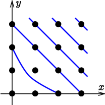
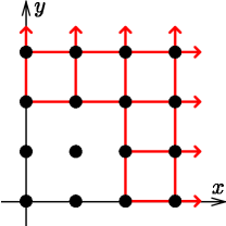
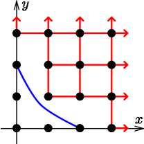
Figure 1. Each line segment above represents a binomial element of the ideal $I$ in Example 3.12 (left) and its mesoprimary components whose associated mesoprime is the maximal monomial ideal (middle and right). In particular, each connected component represents a monomial equivalence class modulo the given ideal.

Remark 3.13.

The difficulty in computing the coprincipal components of an ideal $I$ in Theorem 3.11 is in locating the essential witnesses of $I$. Indeed, once a witness $x^{m}$ is known, computing the coprincipal component $W_{x^{m}}^{\sigma}(I)$ amounts to computing a saturation and the monomial ideal $M_{x^{m}}^{\sigma}(I)$, which is simply the intersection of the irreducible monomial ideals whose quotients have a maximal nonzero monomial of the form $x^{m^{\prime}}$ with $x^{m^{\prime}}-\lambda x^{m}\in I$ for some $\lambda\in\Bbbk$. $\hexagon$

Theorem 3.11 and Proposition 3.4 produce a primary decomposition of any binomial ideal, and make no assumptions on the field $\Bbbk$. It is also possible to produce an irreducible decomposition using the underlying monoid congruence; see [KMO16] for details on this construction.

Theorem 3.14 ([KM14, Theorems 15.6 and 15.11]).

Fix a binomial ideal $I\subseteq\Bbbk[Q]$. Each associated prime of $I$ is minimal over some associated mesoprime of $I$. If $\Bbbk={\overline{\Bbbk}}$ is algebraically closed, then refining any mesoprimary decomposition of $I$ by canonical primary decomposition of its components yields a binomial primary decomposition of $I$.

4. Toral and Andean mesoprimary components

As we have seen before, the assumption that a binomial ideal $I$ is $A$-homogeneous carries with it a significant simplification of the definition of witness from [KM14]. In general, the primary components of an $A$-homogeneous ideal are $A$-homogeneous. If $I$ is $A$-homogeneous, then the coprincipal components from 3.9 are $A$-homogeneous as well, since taking colon with monomials preserves the grading. Thus, any $A$-homogeneous binomial ideal has an $A$-homogeneous mesoprimary decomposition by Theorem 3.11.

Among all $A$-homogeneous binomial prime ideals, the toric ideal $I_{A}$ (the lattice ideal corresponding to the saturated lattice $\ker_{\mathbb{Z}}(A)$ and the trivial character) is of particular interest. An important property of this ideal is that it is finely graded, meaning that the $A$-graded Hilbert function of $\Bbbk[{\mathbb{N}}^{n}]/I_{A}$ is either $0$ or $1$. It was noted in [DMMa, DMMb] that when primary decomposing an $A$-homogeneous binomial ideal, components corresponding to associated primes which are “close” to finely graded are easier to compute ([DMMb, Theorem 4.13]). This behavior subdivides the $A$-homogeneous binomial primes into two classes (Definition 4.2), namely toral (close to toric ideals) and Andean (see Remark 4.3), according to the behavior of their $A$-homogeneous Hilbert function. In this section, we examine the $A$-graded Hilbert functions of mesoprimes and mesoprimary ideals in the same spirit.

For $\sigma\subset[n]$, denote by $A_{\sigma}$ the matrix consisting of the columns of $A$ indexed by $\sigma$.

Lemma 4.1.

For an $A$-homogeneous ($\sigma$-cellular) mesoprimary ideal $I\subset\Bbbk[{\mathbb{N}}^{n}]$, the following are equivalent.

1. The $A$-graded Hilbert function of $\Bbbk[{\mathbb{N}}^{n}]/I$ is bounded above.

2. If $L\subset{\mathbb{Z}}^{\sigma}$ is the lattice underlying $I_{\textnormal{lat}}=I\cap\Bbbk[{\mathbb{N}}^{\sigma}]$, then $\operatorname{sat}(L)=\ker_{\mathbb{Z}}(A_{\sigma})$.

3. $\dim(\Bbbk[{\mathbb{N}}^{n}]/I)={\rm rank\,}(A_{\sigma})$.

Proof.

Since passing to an algebraic closure of $\Bbbk$ changes neither the $A$-graded Hilbert function nor the dimension of $\Bbbk[{\mathbb{N}}^{n}]/I$, we assume for convenience that $\Bbbk$ is algebraically closed. By Proposition 3.4, if $I_{\textnormal{lat}}$ has primary decomposition $\cap_{j=1}^{g}I_{j}$, where $I_{j}$ are lattice ideals whose underlying lattice is ${\rm Sat}(L)$, then $I=\cap_{j=1}^{g}(I+I_{j})$ is the (binomial) primary decomposition of $I$. By Theorem 2.7, $\dim(\Bbbk[{\mathbb{N}}^{\sigma}]/I_{j})=|\sigma|-{\rm rank\,}(L)$.

We first consider the case that $L$ is saturated, so that $I$ is primary to (the prime ideal) $I_{\textnormal{lat}}+{\mathfrak{m}}_{\sigma^{c}}$. In this case, proceeding as in [DMMa, Example 4.6], $\Bbbk[{\mathbb{N}}^{n}]/I$ has a finite filtration whose successive quotients are torsion free modules of rank $1$ over the affine semigroup ring $\Bbbk[{\mathbb{N}}^{n}]/(I_{\textnormal{lat}}+{\mathfrak{m}}_{\sigma^{c}})$. By induction on the length of this filtration we reduce the proof to the case when $I$ is prime, in which case all the above conditions are clearly equivalent.

When $I$ is not necessarily primary, the $A$-homogeneous maps

$$\Bbbk[{\mathbb{N}}^{n}]/I\twoheadrightarrow\Bbbk[{\mathbb{N}}^{n}]/(I+I_{j})\qquad\textnormal{and}\qquad\Bbbk[{\mathbb{N}}^{n}]/I\hookrightarrow\bigoplus_{j=1}^{g}\Bbbk[{\mathbb{N}}^{n}]/(I+I_{j})$$

imply that the $A$-graded Hilbert function of $\Bbbk[{\mathbb{N}}^{n}]/I$ is bounded below by the $A$-graded Hilbert function of $\Bbbk[{\mathbb{N}}^{n}]/(I+I_{1})$ and bounded above by the sum of the $A$-graded Hilbert functions of $\Bbbk[{\mathbb{N}}^{n}]/(I+I_{j})$ for $j=1,\dots,g$.

Note that the $A$-graded Hilbert functions of the rings $\Bbbk[{\mathbb{N}}^{n}]/(I+I_{j})$ are either all bounded or all unbounded, by the previous argument in the primary case, since the underlying lattice is the same. Therefore, the $A$-graded Hilbert function of $\Bbbk[{\mathbb{N}}^{n}]/I$ is bounded above if and only if the $A$-graded Hilbert function of $\Bbbk[{\mathbb{N}}^{n}]/(I+I_{1})$ is bounded above. Noting that the rings $\Bbbk[{\mathbb{N}}^{n}]/(I+I_{j})$, $j=1,\dots,g$, have the same dimension, which thus equals $\dim(\Bbbk[{\mathbb{N}}^{n}]/I)$, the proof of the desired equivalences is reduced to the primary case. ∎

Definition 4.2.

Let $I\subset\Bbbk[{\mathbb{N}}^{n}]$ be an $A$-homogeneous mesoprimary ideal. We say that $\Bbbk[{\mathbb{N}}^{n}]/I$ (or $I$ itself) is toral if one of the equivalent conditions of Lemma 4.1 is satisfied. Otherwise, $\Bbbk[{\mathbb{N}}^{n}]/I$ and $I$ are called Andean. Note that both of these properties depend on the $A$-grading.

Remark 4.3.

The name “Andean” is a pictorial description of the grading of quotients by Andean ideals. If $I\subseteq\Bbbk[{\mathbb{N}}^{n}]$ is an Andean prime, the set

$$\{\beta\in{\mathbb{Z}}^{d}\mid(\Bbbk[{\mathbb{N}}^{n}]/I)_{\beta}\neq 0\}$$

consists of the lattice points on a translate of a face of the cone ${\mathbb{R}}_{>0}A$ (not necessarily a proper face). Since the Hilbert function is unbounded, the picture of a very high, long and thin mountain range comes to mind. See also [DMMb, Remark 5.3]. $\hexagon$

Example 4.4 ([DMMb, Example 1.7]).

Consider $I=\langle xz-y,xw-y\rangle=\langle z-w,xw-y\rangle\cap\langle x,y\rangle$, graded such that $\deg(x)=(1,0)$, $\deg(y)=(1,1)$, and $\deg(z)=\deg(w)=(0,1)$. We claim the first component is toral and the second is Andean.

Indeed, $\Bbbk[x,y,z,w]/\langle z-w,xw-y\rangle$ has Hilbert function 1 in degree $(a,b)\in{\mathbb{Z}}_{\geq 0}^{2}$. On the other hand, the Hilbert function of $\Bbbk[x,y,z,w]/\langle x,y\rangle=\Bbbk[z,w]$ is 0 in degree $(a,b)$ whenever $a>0$, while in degree $(0,b)$ with $b\geq 0$, the Hilbert function is $b+1$, which is unbounded.

To make this more interesting, one can consider the Hilbert function of $\Bbbk[x,y,z,w]/I$. In this case, the Hilbert function is 1 in degree $(a,b)$ when $a$ is positive, and $b+1$ when $a=0$.

Corollary 4.5.

Each prime associated to a toral mesoprimary ideal is toral, and every prime associated to an Andean mesoprimary ideal is Andean.

If $I$ is mesoprimary, then $I$ is either toral or Andean. We note that $I$ is toral if and only if $\Bbbk[{\mathbb{N}}^{n}]/I$ is a toral module in the sense of [DMMb, Definition 4.1]; and $I$ is Andean if and only if $\Bbbk[{\mathbb{N}}^{n}]/I$ is an Andean module in the sense of [DMMb, Definition 5.1].

Lemma 4.6.

Suppose $I\subseteq J$ are $A$-homogeneous mesoprimary ideals. If $I$ is toral, then so is $J$.

Proof.

Note that the $A$-graded Hilbert function of $\Bbbk[{\mathbb{N}}^{n}]/J$ is bounded above by the $A$-graded Hilbert function of $\Bbbk[{\mathbb{N}}^{n}]/I$. If the latter is bounded, then so is the former. ∎

A binomial ideal may have both Andean and toral minimal and embedded primes, and the minimal prime corresponding to a toral embedded prime may be Andean. However, any embedded prime corresponding to a toral minimal prime must be toral. See the examples below.

On the other hand, whenever a cellular $A$-homogeneous binomial ideal $I$ has at least one Andean component, then all of the toral primes must be embedded. Indeed, the minimal primes of $I$ correspond to the minimal primes of the lattice ideal $I\cap\Bbbk[{\mathbb{N}}^{\sigma}]$, and therefore, once this is Andean, all the minimal primes are Andean, and any remaining components (including every toral component) must be embedded.

Example 4.7.

For cellular binomial ideals, toral primes may be embedded in Andean primes, but not the other way around. For example, the cellular ideal $I\subset\Bbbk[a,b,c,d,x,y]$ given by

$$I=\langle ad-bc,x(ac-b^{2}),x(bd-c^{2}),y(ac-b^{2}),y(bd-c^{2}),x^{2},xy,y^{2}\rangle$$

is positively graded via $\deg(a)=\left[\begin{smallmatrix}1\\ 0\end{smallmatrix}\right]$, $\deg(b)=\left[\begin{smallmatrix}1\\ 1\end{smallmatrix}\right]$, $\deg(c)=\left[\begin{smallmatrix}1\\ 2\end{smallmatrix}\right]$, $\deg(d)=\left[\begin{smallmatrix}1\\ 3\end{smallmatrix}\right]$, $\deg(x)=\left[\begin{smallmatrix}1\\ 4\end{smallmatrix}\right]$, and $\deg(y)=\left[\begin{smallmatrix}1\\ 5\end{smallmatrix}\right]$.

The ideal $I$ has three coprincipal components in the decomposition from Theorem 3.11, with essential witnesses $1$, $x$, and $y$. The first yields an Andean component, and the remaining two components have the same associated (toral) mesoprime with different Artinian parts. In particular,

$$\begin{array}[]{rcl}I&=&\langle ad-bc,x,y\rangle\cap\langle ad-bc,ac-b^{2},bd-c^{2},x^{2},y\rangle\cap\langle ad-bc,ac-b^{2},bd-c^{2},x,y^{2}\rangle\\ &=&\langle ad-bc,x,y\rangle\cap\langle ad-bc,ac-b^{2},bd-c^{2},x^{2},xy,y^{2}\rangle\\ \end{array}$$

upon combining the last two coprincipal components to a single mesoprimary component. See Figure 2 for picture of the nilpotent monomials of $I$. $\hexagon$

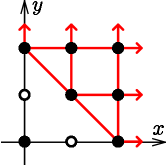
Figure 2. Depicted above are the nilpotent monomial equivalence classes modulo the cellular ideal $I$ in Example 4.7. The origin is a witness for a principal lattice ideal, and the monomials $x$ and $y$ are both witnesses for the twisted cubic.

5. Some combinatorial savings when computing toral components

An important result in [DMMa] is that toral primary components of $A$-homogeneous binomial ideals are easier to compute than Andean ones. This statement is [DMMa, Theorem 4.13], which contains a minor error (see Remark 5.3).

We first recall how primary components are computed in [DMMa]. Suppose that $\sigma\subseteq[n]$, $I(\rho)$ is a prime lattice ideal in $\Bbbk[{\mathbb{N}}^{\sigma}]$, and $P=I(\rho)+{\mathfrak{m}}_{\sigma^{c}}$ is a toral associated prime of an $A$-homogeneous binomial ideal $I$. Then [DMMa, Theorem 3.2] states that in the case that $\Bbbk$ is an algebraically closed field of characteristic zero, the $P$-primary component of $I$ may be chosen of the form

(5.1) $$\big{(}(I+I(\rho)+K):(\prod_{i\in\sigma}x_{i})^{\infty}\big{)}+M$$

where $K,M\subseteq\Bbbk[{\mathbb{N}}^{\sigma^{c}}]$, $K$ is generated by sufficiently high powers of the variables $x_{j}$, $j\notin\sigma$, and $M$ is a monomial ideal computed combinatorially. If $P$ is a minimal prime of $I$, then we may choose $K=\langle 0\rangle$.

We remark that the ideal $M$ above does not necessarily contain all monomials belonging to the corresponding primary component. Even when $P$ is minimal, $\big{(}(I+I(\rho)):(\prod_{i\in\sigma}x_{i})^{\infty}\big{)}$ may contain monomials in $\Bbbk[{\mathbb{N}}^{\sigma^{c}}]$ that belong neither to $I$ nor to $M$.

Example 5.1.

Let $I=\langle z^{2}-w^{2},x(z-w),x^{2}\rangle\subset\Bbbk[x,z,w]$, with the usual ${\mathbb{Z}}$-grading on the polynomial ring. Then the primary component associated to the minimal prime $\langle z+w,x\rangle$ is $\langle z+w,x\rangle$. In this case, the monomial ideal $M$ from (5.1) is $M=\langle x^{2}\rangle$; the monomial $x$ comes from performing $((I+\langle z+w\rangle):(zw)^{\infty})$. $\hexagon$

The monomial ideal $M$ from (5.1) is computed by considering a congruence on the monoid ${\mathbb{Z}}^{\sigma}\times{\mathbb{N}}^{\sigma^{c}}$. The gist of [DMMa, Theorem 4.13] is that, for toral primes, the computation of the monomial ideal $M$ can be performed by considering a congruence on the (much smaller) monoid ${\mathbb{N}}^{\sigma^{c}}$. This leads to significant combinatorial savings when computing toral primary components.

Theorem 5.2.

Let $I$ be an $A$-homogeneous binomial ideal in $\Bbbk[{\mathbb{N}}^{n}]$, where $\Bbbk$ is an algebraically closed field of characteristic zero. Let $\sigma\subseteq[n]$, $I(\rho)\subseteq\Bbbk[{\mathbb{N}}^{\sigma}]$ a prime lattice ideal corresponding to a character $\rho:L\to\Bbbk^{*}$, and assume that $P=I(\rho)+{\mathfrak{m}}_{\sigma^{c}}$ is a toral associated prime of $I$. Let $\nu=(\nu_{j})_{j\in\sigma}\in(\Bbbk^{*})^{\sigma}$ be a zero of $I\cap\Bbbk[{\mathbb{N}}^{\sigma}]$, and set $\overline{I}=I\cdot\Bbbk[{\mathbb{N}}^{n}]/\langle x_{j}-\nu_{j}\mid j\in\sigma\rangle$. We consider $\overline{I}$ as an ideal in $\Bbbk[{\mathbb{N}}^{\sigma}]$. Then a valid choice for the $P$-primary component of $I$ is

(5.2) $$\big{(}(I+I(\rho)+K):(\prod_{i\in\sigma}x_{i})^{\infty}\big{)}+\overline{M},$$

where $K$ is an ideal generated by sufficiently high powers of the variables indexed by $\sigma^{c}$, and $\overline{M}$ is the monomial ideal combinatorially produced by [DMMa, Theorem 3.2] for the associated prime ${\mathfrak{m}}_{\sigma^{c}}$ of $\overline{I}$.

Remark 5.3.

We note that the statement of [DMMa, Theorem 4.13] contains a minor error. Instead of setting the variables indexed by $\sigma$ to values given by a zero of $I\cap\Bbbk[{\mathbb{N}}^{\sigma}]$, as we do in Theorem 5.2, those variables are set to $1$, which is a valid choice only when $(1)_{i\in\sigma}\in(\Bbbk^{*})^{\sigma}$ is a root of $I\cap\Bbbk[{\mathbb{N}}^{\sigma}]$. If this is not the case, then setting the variables indexed by $\sigma$ to $1$ introduces constants to $\overline{I}$. The proof of [DMMa, Theorem 4.13] is correct, once the statement is suitably modified. $\hexagon$

It has been one of the goals of this project to provide an analogous result for computing witnesses and coprincipal or mesoprimary components of $A$-homogeneous binomial ideals corresponding to toral mesoprimes. A general statement is unfortunately out of reach.

Remark 5.4.

We emphasize that the monomials of an associated mesoprime cannot necessarily be obtained by evaluating the $\sigma$-variables. For example, the mesoprimary decomposition of the ideal $I=\langle z^{2}-w^{2},x(z-w),x^{2}\rangle\subset\Bbbk[x,z,w]$ constructed in Theorem 3.11 is

$$I=\langle z^{2}-w^{2},x\rangle\cap\langle z-w,x^{2}\rangle,$$

and both components have $\langle z-w,x\rangle$ as an associated prime. As such, the primary decomposition

$$I=\langle z+w,x\rangle\cap\langle z-w,x^{2}\rangle$$

results from taking the canonical primary decomposition of each mesoprimary component and collecting both components with associated prime $\langle z-w,x\rangle$. $\hexagon$

While there may not be a general result along the lines of Theorem 5.2 for mesoprimary decomposition, we do provide in Theorem 5.10 a special case in which lower-dimensional combinatorics can be used for computations.

We start by introducing terminology and providing auxiliary results.

Definition 5.5.

The support of a polynomial $h$, denoted $\operatorname{supp}(h)$, is the set of monomials that appear in $h$ with nonzero coefficient.

Convention 5.6.

Until the end of this section, we use the following notation and assumptions. Let $I$ be an $A$-homogeneous binomial ideal, where $A$ is a $d\times n$ matrix of rank $d<n$. Let $\sigma\subset[n]$, with $|\sigma|=d$, be such that the matrix $A_{\sigma}$ consisting of the columns of $A$ indexed by $\sigma$ has full rank $d$. We assume that $(1)_{i\in\sigma}\in\Bbbk^{\sigma}$ is a zero of $I\cap\Bbbk[{\mathbb{N}}^{\sigma}]$. Let $\overline{I}$ be the ideal $I\cdot(\Bbbk[{\mathbb{N}}^{n}]/\langle x_{i}-1\mid i\in\sigma\rangle)$, considered as an ideal in $\Bbbk[{\mathbb{N}}^{\sigma^{c}}]$.

Proposition 5.7.

Under the notation and assumptions of Convention 5.6, if $g=\sum_{i=1}^{r}\lambda_{i}x^{u_{i}}$, where $\lambda_{i}\in\Bbbk^{*}$ and $u_{i}\in{\mathbb{N}}^{\sigma^{c}}$ for $i=1,\dots,r$, then $g\in\overline{I}$ if and only if there are $v_{1},\dots,v_{r}\in{\mathbb{N}}^{\sigma}$ such that $f=\sum_{i=1}^{r}\lambda_{i}x^{u_{i}}x^{v_{i}}\in I$.

Proof.

We note that if $f=\sum_{i=1}^{r}\lambda_{i}x^{u_{i}}x^{v_{i}}$ as above belongs to $I$, then $g=\sum_{i=1}^{r}\lambda_{i}x^{u_{i}}\in\overline{I}$.

Assume $g=\sum_{i=1}^{r}\lambda_{i}x^{u_{i}}\in\overline{I}$. Since $\overline{I}$ is a binomial ideal, there are $\mu_{1},\dots,\mu_{s}\in\Bbbk^{*}$ and binomials $\overline{b}_{1},\dots,\overline{b}_{s}\in\overline{I}\subset\Bbbk[{\mathbb{N}}^{\sigma^{c}}]$, where each $\overline{b}_{i}$ denotes the image in $\overline{I}$ of a binomial $b_{i}\in I$, such that $g=\mu_{1}\overline{b}_{1}+\dots+\mu_{s}\overline{b}_{s}$. We may assume that $b_{1},\dots,b_{s}$ are $A$-homogeneous and no two of them have the same support. Since $A_{\sigma}$ is invertible, we see that if $\overline{b}_{i}$ has one term, then $b_{i}$ has one term. Moreover, we may choose $b_{1},\dots,b_{s}$ in such a way that if $i\neq j$, then $\overline{b}_{i}$ and $\overline{b}_{j}$ have different supports. To see this, suppose that $b_{i}=x^{w}x^{p}-\kappa x^{v}x^{q}$ and $b_{j}=x^{w^{\prime}}x^{p}-\kappa^{\prime}x^{v^{\prime}}x^{q}$, where $p,q\in{\mathbb{N}}^{\sigma^{c}}$, $v,v^{\prime},w,w^{\prime}\in{\mathbb{N}}^{\sigma}$ and $\kappa,\kappa^{\prime}\in\Bbbk$. Since $b_{i}$ and $b_{j}$ are $A$-homogeneous, and $A_{\sigma}$ is invertible, we have that $w-v=w^{\prime}-v^{\prime}$, so that $x^{w^{\prime}}b_{i}$ and $x^{w}b_{j}$ have the same support. If $x^{w^{\prime}}b_{i}=x^{w}b_{j}$, we may use this binomial instead of $b_{i}$ and $b_{j}$. If $x^{w^{\prime}}b_{i}\neq x^{w}b_{j}$, then $x^{w+w^{\prime}}x^{p},x^{v+v^{\prime}}x^{q}\in I$, and we may use these monomials instead of $b_{i}$ and $b_{j}$.

If the binomials $\overline{b}_{1},\dots,\overline{b}_{s}$ have pairwise disjoint supports, then $f=\sum_{i=1}^{s}\mu_{i}b_{i}\in I$ satisfies the required conditions.

Now suppose that $x^{m}\in\Bbbk[{\mathbb{N}}^{\sigma^{c}}]$ belongs to the support of at least two of the binomials $\overline{b}_{i}$. For each $i$ such that $x^{m}$ is in the support of $\overline{b}_{i}$, there exists $x^{q_{i}}\in\Bbbk[{\mathbb{N}}^{\sigma}]$ such that $x^{m}x^{q_{i}}$ is in the support of $b_{i}$. Let $x^{q}\in\Bbbk[{\mathbb{N}}^{\sigma}]$ be the least common multiple of all such $x^{q_{i}}$. Then the coefficient of $x^{m}$ in the sum of the $\mu_{i}\overline{b}_{i}$ over all $\overline{b}_{i}$ containing $x^{m}$ in their support equals the coefficient of $x^{q}x^{m}$ in the sum of the $\mu_{i}x^{q-q_{i}}b_{i}$ over all $b_{i}$ containing a multiple of $x^{m}$ in their support.

If $x^{m}$ is the only monomial appearing the support of more than one $\overline{b_{i}}$, then the polynomial $f$ constructed as the sum over $\overline{b}_{i}$ containing $x^{m}$ of $\mu_{i}x^{q-q_{i}}b_{i}$ plus the sum over $\overline{b}_{i}$ not containing $x^{m}$ of $\mu_{i}b_{i}$ satisfies the required conditions.

If there exists $x^{m^{\prime}}\in\Bbbk[{\mathbb{N}}^{\sigma^{c}}]$, $x^{m^{\prime}}\neq x^{m}$, appearing in the support of more than one of the $\overline{b}_{j}$, and $x^{m}$, $x^{m^{\prime}}$ are the only two monomials with this property, we repeat the same procedure as before, obtaining binomials $\mu_{j}x^{q^{\prime}-q^{\prime}_{j}}b_{j}$, with the proviso that if the support of $\overline{b}_{\ell}$ equals $\{x^{m},x^{m^{\prime}}\}$, then we use

$$f=\mu_{\ell}x^{q+q^{\prime}-q_{\ell}-q^{\prime}_{\ell}}b_{\ell}+\sum_{\begin{subarray}{c}i\neq\ell\\ x^{m}\in\operatorname{supp}(\overline{b}_{i})\end{subarray}}\mu_{i}x^{q+q^{\prime}-q_{\ell}^{\prime}-q_{i}}b_{i}+\sum_{\begin{subarray}{c}j\neq\ell\\ x^{m^{\prime}}\in\operatorname{supp}(\overline{b}_{j})\end{subarray}}\mu_{j}x^{q+q^{\prime}-q_{\ell}-q^{\prime}_{j}}b_{j}+\sum_{x^{m},x^{m^{\prime}}\notin\operatorname{supp}(\overline{b}_{k})}\mu_{k}b_{k}.$$

If there is $x^{m^{\prime\prime}}\in\Bbbk[{\mathbb{N}}^{\sigma^{c}}]$, different from $x^{m}$ and $x^{m^{\prime}}$ that appears in more than one support, we repeat the procedure, taking care that if there is a binomial $\overline{b}_{i}$ with support $\{x^{m},x^{m^{\prime\prime}}\}$ and/or a binomial $\overline{b}_{j}$ with support $\{x^{m^{\prime}},x^{m^{\prime\prime}}\}$, then all of the binomials $b_{k}$ involving multiples of $x^{m}$ or $x^{m^{\prime}}$ need to be multiplied by additional monomials in $\Bbbk[{\mathbb{N}}^{\sigma}]$.

Continuing in this manner, we obtain the desired $f$. ∎

Proposition 5.8.

Under the assumptions and notation of Convention 5.6, if $p\in\Bbbk[{\mathbb{N}}^{n}]$ is an $A$-homogeneous polynomial not belonging to $I_{\sigma}=\big{(}I:(\prod_{i\in\sigma}x_{i})^{\infty}\big{)}$, then its image $\overline{p}$ in $\Bbbk[{\mathbb{N}}^{\sigma^{c}}]$ under the map that sets to $1$ the variables indexed by $\sigma$ does not belong to $\overline{I}$.

Proof.

We prove the contrapositive statement by induction on the cardinality of the support of $p$. If $p=\lambda x^{u}x^{m}$, where $\lambda\in\Bbbk^{*},x^{u}\in\Bbbk[{\mathbb{N}}^{\sigma}],x^{m}\in\Bbbk[{\mathbb{N}}^{\sigma^{c}}]$, and $\overline{p}=\lambda x^{m}\in\overline{I}$, apply Proposition 5.7 to obtain a monomial $x^{v}\in\Bbbk[{\mathbb{N}}^{\sigma}]$ such that $\lambda x^{v}x^{m}\in I$. This implies $x^{m}\in I_{\sigma}$, and therefore $p\in I_{\sigma}$.

Now let $p=\sum_{i=1}^{r}\lambda_{i}x^{u_{i}}x^{m_{i}}\in\Bbbk[{\mathbb{N}}^{n}]$, where $\lambda_{i}\in\Bbbk^{*},x^{u_{i}}\in\Bbbk[{\mathbb{N}}^{\sigma}],x^{m_{i}}\in\Bbbk[{\mathbb{N}}^{\sigma^{c}}]$ for $i=1,\dots,r$ and $r\geq 2$. Assume that $\overline{p}\in\overline{I}$. By Proposition 5.7, there are $x^{v_{1}},\dots,x^{v_{r}}\in\Bbbk[{\mathbb{N}}^{\sigma}]$ such that $p^{\prime}=\sum\lambda_{i}x^{v_{i}}x^{m_{i}}\in I$. Since $I$ is $A$-homogeneous, the homogeneous components of $p^{\prime}$ belong to $I$. Denote by $q$ one such component. As the matrix $A_{\sigma}$ is invertible, we can find monomials $x^{u},x^{v}\in\Bbbk[{\mathbb{N}}^{\sigma}]$ such that $x^{u}p$ and $x^{v}q$ have the same $A$-degree. Now, let $i$ be such that $\lambda_{i}x^{v_{i}}x^{m_{i}}$ is a monomial in $q$. Then $x^{u}x^{u_{i}}x^{m_{i}}$ and $x^{v}x^{v_{i}}x^{m_{i}}$ have the same $A$-degree. Using again the fact that $A_{\sigma}$ is invertible, we see that $u+u_{i}=v+v_{i}$. This implies that the support of $x^{u}p-x^{v}q$ is strictly contained in the support of $p$, and since $q\in I$, the image $\overline{q}$ of $x^{v}q$ under setting to $1$ the variables indexed by $\sigma$ belongs to $\overline{I}$. By induction, $x^{u}p-x^{v}q\in I_{\sigma}$ Moreover, since $q\in I\subset I_{\sigma}$, we see that $x^{u}p\in I_{\sigma}$, and by definition of $I_{\sigma}$, this implies that $p\in I_{\sigma}$. ∎

Definition 5.9.

Fix $\sigma\subset[n]$ and a binomial ideal $I\subset\Bbbk[{\mathbb{N}}^{n}]$. Set $I_{\sigma}=\big{(}I:(\prod_{i\in\sigma}x_{i})^{\infty}\big{)}$.

1. A weak monomial $I$-witness for ${\mathfrak{m}}_{\sigma^{c}}$ is a monomial $x^{w}\in\Bbbk[{\mathbb{N}}^{\sigma^{c}}]$, $x^{w}\notin I$, such that there exists $x^{m}\in\Bbbk[{\mathbb{N}}^{\sigma}]$ with the property that for each $i\notin\sigma$, there are a monomial $x^{q_{i}}$ and a scalar $\lambda_{i}\in\Bbbk^{*}$ such that $x_{i}(x^{m}x^{w}-\lambda_{i}x^{q_{i}})\in I_{\sigma}$ but $x^{m}x^{w}-\lambda_{i}x^{q_{i}}\notin I_{\sigma}$.

2. A weak monomial $I$-witness $x^{w}$ for ${\mathfrak{m}}_{\sigma^{c}}$ is essential if there is a polynomial $p\in\Bbbk[{\mathbb{N}}^{n}]$, $p\notin I_{\sigma}$, and a monomial $x^{v}\in\Bbbk[{\mathbb{N}}^{\sigma}]$ such that $x^{v}x^{w}$ is a monomial in $p$, and $x_{j}p\in I_{\sigma}$ for all $j\notin\sigma$.

The difference between Definition 3.7 and Definition 5.9 is that the ideal $I$ is not assumed to be positively graded. This is a profound difference, as weak monomial witnesses are not monomial witnesses in the sense of [KM14], because the conditions on divisibility imposed by the definitions in [KM14] are not (necessarily) satisfied.

Theorem 5.10.

Under the assumptions and notation of Convention 5.6, a monomial $x^{w}\in\Bbbk[{\mathbb{N}}^{\sigma^{c}}]$ is an (essential) monomial $I$-witness for ${\mathfrak{m}}_{\sigma^{c}}\subset\Bbbk[{\mathbb{N}}^{n}]$ if and only if it is a weak (essential) monomial $\overline{I}$-witness for ${\mathfrak{m}}_{\sigma^{c}}\subset\Bbbk[{\mathbb{N}}^{\sigma^{c}}]$.

Proof.

Let $x^{w}\in\Bbbk[{\mathbb{N}}^{\sigma^{c}}]$ be a monomial $I$-witness for ${\mathfrak{m}}_{\sigma^{c}}\subset\Bbbk[{\mathbb{N}}^{n}]$. Using Proposition 5.8, we see that the images under setting to $1$ the variables indexed by $\sigma$ of the auxiliary binomials required for $x^{w}$ to be a monomial $I$-witness, satisfy the conditions required for $x^{w}$ to be a weak monomial $\overline{I}$-witness. If $x^{w}$ is an essential monomial $I$-witness, the image of the auxiliary polynomial $p$ serves to verify that $x^{w}$ is an essential weak monomial $\overline{I}$-witness.

Now assume that $x^{w}$ is a weak monomial $\overline{I}$-witness for ${\mathfrak{m}}_{\sigma^{c}}\subset\Bbbk[{\mathbb{N}}^{\sigma^{c}}]$, and for each $i\in\sigma^{c}$, let $\lambda_{i}\in\Bbbk^{*}$ and $x^{q_{i}}\in\Bbbk[{\mathbb{N}}^{\sigma}]$ such that $x_{i}(x^{w}-\lambda_{i}x^{q_{i}})\in\overline{I}$ but $x^{w}-\lambda_{i}x^{q_{i}}\notin\overline{I}$. By Propositions 5.7 and 5.8 there are monomials $x^{u_{i}},x^{v_{i}}\in\Bbbk[{\mathbb{N}}^{\sigma}]$ such that $x_{i}(x^{u_{i}}x^{w}-\lambda_{i}x^{v_{i}}x^{q_{i}})\in I\subset I_{\sigma}$ and $(x^{u_{i}}x^{w}-\lambda_{i}x^{v_{i}}x^{q_{i}})\notin I_{\sigma}$. Taking $x^{u}$ to be the least common multiple of the $x^{u_{i}}$, we see that the binomials $x^{u}x^{w}-\lambda_{i}x^{u-u_{i}}x^{v_{i}}x^{q_{i}}$ satisfy the properties necessary to ensure that $x^{w}$ is a monomial $I$-witness for ${\mathfrak{m}}_{\sigma^{c}}\subset\Bbbk[{\mathbb{N}}^{n}]$.

Finally, if $x^{m}$ is a weak essential monomial $\overline{I}$-witness for ${\mathfrak{m}}_{\sigma^{c}}\subset\Bbbk[{\mathbb{N}}^{\sigma^{c}}]$, then in particular $x^{w}$ is a weak monomial $\overline{I}$-witness for ${\mathfrak{m}}_{\sigma^{c}}\subset\Bbbk[{\mathbb{N}}^{\sigma^{c}}]$, and by the previous argument, it is a monomial $I$-witness for ${\mathfrak{m}}_{\sigma^{c}}\subset\Bbbk[{\mathbb{N}}^{n}]$. Now let $g=\sum_{i=1}^{r}\mu_{i}x^{m_{i}}\in\Bbbk[{\mathbb{N}}^{\sigma^{c}}]$, $\mu_{1},\dots,\mu_{r}\in\Bbbk^{*}$, such that $g\notin\overline{I}$, $m_{1}=w$, and $x_{i}g\in\overline{I}$ for all $i\in\sigma^{c}$. Fix $i_{0}\in\sigma^{c}$. By Propositions 5.7 and 5.8 applied to $x_{i_{0}}g$, there are monomials $x^{v_{1}},\dots,x^{v_{r}}\in\Bbbk[{\mathbb{N}}^{\sigma}]$ such that $p^{\prime}=\sum_{i=1}^{r}\mu_{i}x^{v_{i}}x^{m_{i}}\notin I_{\sigma}$ and $x_{i_{0}}p^{\prime}\in I\subset I_{\sigma}$. By Proposition 5.8, if $x_{j}\in\sigma^{c}$, $j\neq i_{0}$, the fact that $x_{j}g\in\overline{I}$ implies that $x_{j}p^{\prime}\in I_{\sigma}$. Now let $p$ be the $A$-homogeneous component of $p^{\prime}$ containing the monomial $x^{v_{1}}x^{m_{1}}=x^{v_{1}}x^{w}$. Since $I$ and $I_{\sigma}$ are $A$-homogeneous, the polynomial $p$ satisfies the conditions necessary to ensure that $x^{m}$ is an essential monomial $I$-witness for ${\mathfrak{m}}_{\sigma^{c}}\subset\Bbbk[{\mathbb{N}}^{n}]$. ∎

6. The toral part of a binomial primary decomposition

As [DMMb, Proposition 6.4] shows, it sometimes makes sense to discard the Andean components of an $A$-homogeneous binomial ideal. The goal of this section is to show that this process may not result in a binomial ideal (Example 6.3).

Definition 6.1.

Fix an $A$-homogeneous binomial ideal $I\subset\Bbbk[{\mathbb{N}}^{n}]$, where $\Bbbk$ is algebraically closed. Let $I=\cap_{\ell=1}^{r}J_{\ell}$ and a binomial primary decomposition, where $J_{1},\dots,J_{t}$ are toral and $J_{t+1},\dots,J_{r}$ are Andean. The toral part of (this decomposition of) $I$, denoted $I_{\textnormal{toral}}$, equals the intersection $\cap_{\ell}^{t}J_{\ell}$ of the toral components (cf. [DMMb, Proposition 6.4]).

Since embedded primary components are not uniquely determined, the ideal $I_{\textnormal{toral}}$ in Definition 6.1 depends on the primary decomposition unless all the toral associated primes of $I$ are minimal.

Lemma 6.2.

Let $I$ be an $A$-homogeneous binomial ideal in $\Bbbk[{\mathbb{N}}^{n}]$, and let $I=\cap_{\ell=1}^{p}I_{\ell}$ be a mesoprimary decomposition of $I$. Assume that $I_{1},\dots,I_{q}$ are toral and $I_{q+1},\dots,I_{p}$ are Andean, and consider $J=\cap_{\ell=1}^{q}I_{\ell}$. Then $J$ equals $I_{\textnormal{toral}}$ for the primary decomposition of $I$ obtained by primary decomposing the mesoprimary components $I_{\ell}$.

Proof.

The reason this is not immediate is that, when the mesoprimary components $I_{\ell}$ are primary decomposed, some of the resulting primary ideals may not be components of $I$. The question of how to eliminate possible redundancies in this process is a subtle one [KM14, Remark 16.11]; however, in this case, we need only observe that cancellations cannot occur between Andean and toral mesoprimary components, as the corresponding collections of associated primes are disjoint. ∎

Example 6.3.

It is possible for the toral part of a binomial primary decomposition to not be a binomial ideal, even when all the toral associated primes are minimal. Let

$$I=\langle x_{3}^{4}x_{5}-x_{4}^{3}x_{6}^{3},x_{3}^{5}x_{6}-x_{4}^{5}x_{5}^{2},x_{1}x_{5}^{3}-x_{2}^{4}x_{6},x_{1}^{4}x_{6}^{5}-x_{2}^{2}x_{5}^{2}\rangle\subseteq\Bbbk[x_{1},\dots,x_{6}].$$

The ideal $I$ is (positively) $A$-homogeneous, for the matrix $A=\left[\begin{smallmatrix}5&5&-11&-13&5&0\\ 60&73&-130&-160&82&14\end{smallmatrix}\right]$ and has seven associated primes. Five of these are toral, and all those are minimal, which means that their corresponding primary components are uniquely determined. Consequently, $I_{\textnormal{toral}}$ is independent of the primary decomposition of $I$. In this example, it can be verified using the Macaulay2 package Binomials that $I_{\textnormal{toral}}$ is not binomial. $\hexagon$

Remark 6.4.

While working on this article, we found a small error in [DMMa, Example 4.10].

In [DMMa, Example 4.10], it is incorrectly claimed that the dimension of any associated prime of a lattice basis ideal $I$ is at least the rank $d$ of its grading matrix. This error leads to the false conclusion that all toral associated primes of a lattice basis ideal $I$ have dimension exactly $d$ and are therefore minimal. Consequently, the description in [DMMa] does not capture all of the toral associated primes of a lattice basis ideal (or even all of the minimal ones).

Moreover, toral primes of a lattice basis ideal may be embedded. (For example, $\langle x_{1},x_{2},x_{4}\rangle$ is a toral embedded prime of the lattice basis ideal

$$I=\langle x_{1}^{3}-x_{2}^{2}x_{3},x_{1}^{2}-x_{2}x_{4}^{5},x_{1}^{2}-x_{2}^{2}x_{5}^{3}\rangle\subset\Bbbk[x_{1},\dots,x_{5}]$$

with grading matrix $A=\left[\begin{smallmatrix}\phantom{-}5&\phantom{-}5&5&1&0\\ -3&-6&3&0&2\end{smallmatrix}\right]$ .) For this reason, a complete description of the toral associated primes of a lattice basis ideal is not feasible using only the combinatorics of its defining matrix matrix, since, as [HS, Example 3.1] shows, it is not possible to determine the embedded primes of a lattice basis ideals from the sign patterns of the entries of the underlying matrix.

We remark that this error in [DMMa] is carried over to [DMMb, Section 7], although the only false result there is [DMMb, Lemma 7.2]. This affects the statements of [DMMb, Lemma 7.4, Proposition 7.6, Theorem 7.14, Theorem 7.18, Corollary 7.25], in which a certain matrix $M$ is assumed to be square invertible, an assumption that comes from the incorrect [DMMb, Lemma 7.2]. Fortunately, none of these results actually need the assumptions on $M$, and the only modification needed is in the verification that the second display of the proof of of [DMMb, Theorem 7.14] is valid. We also point out that the display in [DMMb, Example 3.7] should read $\mathscr{C}_{\rho,J}=((I(B)+I_{\rho}):\partial_{J}^{\infty})+U_{M}$. $\hexagon$

References

- [DMMa] A. Dickenstein, L. Matusevich, and E. Miller Combinatorics of binomial primary decomposition, Math. Z. 264 (2010), no. 4, 745–763.
- [DMMb] A. Dickenstein, L. Matusevich, and E. Miller Binomial -modules, Duke Math. J. 151 no. 3 (2010), 385–429.
- [ES96] David Eisenbud and Bernd Sturmfels, Binomial ideals, Duke Math. J. 84 (1996), no. 1, 1–45.
- [EM14] Zekiye Sahin Eser and Laura Felicia Matusevich, Decompositions of cellular binomial ideals, J. London Math. Soc. 94 (2016), 409–426.
- [HS] Serkan Hoşten and Jay Shapiro, Primary decomposition of lattice basis ideals, J. Symbolic Comput. 29 (2000), no. 4–5, 625–639.
- [KM14] Thomas Kahle and Ezra Miller, Decompositions of commutative monoid congruences and binomial ideals, Algebra Number Theory 8 (2014), no. 6, 1297–1364.
- [KMO16] T. Kahle, E. Miller and C. O’Neill, Irreducible decomposition of binomial ideals, Compositio Mathematica, 152 (2016), 1319–1332.
- [OS00] Ignacio Ojeda Martínez de Castilla and Ramón Piedra Sánchez, Cellular binomial ideals. Primary decomposition of binomial ideals, J. Symbolic Comput., 30 (2000), No. 4, 383–400.