Parameterized Approximation Algorithms for some Location Problems in Graphs

Abstract

We develop efficient parameterized, with additive error, approximation algorithms for the (Connected) $r$-Domination problem and the (Connected) $p$-Center problem for unweighted and undirected graphs. Given a graph $G$, we show how to construct a (connected) $\big{(}r+\mathcal{O}(\mu)\big{)}$-dominating set $D$ with $|D|\leq|D^{*}|$ efficiently. Here, $D^{*}$ is a minimum (connected) $r$-dominating set of $G$ and $\mu$ is our graph parameter, which is the tree-breadth or the cluster diameter in a layering partition of $G$. Additionally, we show that a $+\mathcal{O}(\mu)$-approximation for the (Connected) $p$-Center problem on $G$ can be computed in polynomial time. Our interest in these parameters stems from the fact that in many real-world networks, including Internet application networks, web networks, collaboration networks, social networks, biological networks, and others, and in many structured classes of graphs these parameters are small constants.

1 Introduction

The (Connected) $r$-Domination problem and the (Connected) $p$-Center problem, along with the $p$-Median problem, are among basic facility location problems with many applications in data clustering, network design, operations research – to name a few. Let $G=(V,E)$ be an unweighted and undirected graph. Given a radius $r(v)\in\mathbb{N}$ for each vertex $v$ of $G$, indicating within what radius a vertex $v$ wants to be served, the $r$-Domination problem asks to find a set $D\subseteq V$ of minimum cardinality such that $d_{G}(v,D)\leq r(v)$ for every $v\in V$. The Connected $r$-Domination problem asks to find an $r$-dominating set $D$ of minimum cardinality with an additional requirement that $D$ needs to induce a connected subgraph of $G$. When $r(v)=1$ for every $v\in V$, one gets the classical (Connected) Domination problem. Note that the Connected $r$-Domination problem is a natural generalization of the Steiner Tree problem (where each vertex $t$ in the target set has $r(t)=0$ and each other vertex $s$ has $r(s)=\operatorname{diam}(G)$). The connectedness of $D$ is important also in network design and analysis applications (e. g. in finding a small backbone of a network). It is easy to see also that finding minimum connected dominating sets is equivalent to finding spanning trees with the maximum possible number of leaves.

The (closely related) $p$-Center problem asks to find in $G$ a set $C\subseteq V$ of at most $p$ vertices such that the value $\max_{v\in V}d_{G}(v,C)$ is minimized. If, additionally, $C$ is required to induce a connected subgraph of $G$, then one gets the Connected $p$-Center problem.

The domination problem is one of the most well-studied NP-hard problems in algorithmic graph theory. To cope with the intractability of this problem it has been studied both in terms of approximability (relaxing the optimality) and fixed-parameter tractability (relaxing the runtime). From the approximability prospective, a logarithmic approximation factor can be found by using a simple greedy algorithm, and finding a sublogarithmic approximation factor is NP-hard [19]. The problem is in fact Log-APX-complete [14]. The Domination problem is notorious also in the theory of fixed-parameter tractability (see, e. g., [11, 18] for an introduction to parameterized complexity). It was the first problem to be shown W[2]-complete [11], and it is hence unlikely to be FPT, i. e., unlikely to have an algorithm with runtime $f(k)n^{c}$ for $f$ a computable function, $k$ the size of an optimal solution, $c$ a constant, and $n$ the number of vertices of the input graph. Similar results are known also for the connected domination problem [17].

The $p$-Center problem is known to be NP-hard on graphs. However, for it, a simple and efficient factor $2$ approximation algorithm exists [16]. Furthermore, it is a best possible approximation algorithm in the sense that an approximation with factor less than $2$ is proven to be NP-hard (see [16] for more details). The NP-hardness of the Connected $p$-Center problem is shown in [20].

Recently, in [7], a new type of approximability result (call it a parameterized approximability result) was obtained: there exists a polynomial time algorithm which finds in an arbitrary graph $G$ having a minimum $r$-dominating set $D$ a set $D^{\prime}$ such that $|D^{\prime}|\leq|D|$ and each vertex $v\in V$ is within distance at most $r(v)+2\delta$ from $D^{\prime}$, where $\delta$ is the hyperbolicity parameter of $G$ (see [7] for details). We call such a $D^{\prime}$ an $(r+2\delta)$-dominating set of $G$. Later, in [13], this idea was extended to the $p$-Center problem: there is a quasi-linear time algorithm for the $p$-Center problem with an additive error less than or equal to six times the input graph’s hyperbolicity (i. e., it finds a set $C^{\prime}$ with at most $p$ vertices such that $\max_{v\in V}d_{G}(v,C^{\prime})\leq\min_{C\subseteq V,|C|\leq p}\max_{v\in V}d_{G}(v,C)+6\delta$). We call such a $C^{\prime}$ a $+6\delta$-approximation for the $p$-Center problem.

In this paper, we continue the line of research started in [7] and [13]. Unfortunately, the results of [7, 13] are hardly extendable to connected versions of the $r$-Domination and $p$-Center problems. It remains an open question whether similar approximability results parameterized by the graph’s hyperbolicity can be obtained for the Connected $r$-Domination and Connected $p$-Center problems. Instead, we consider two other graph parameters: the tree-breadth $\rho$ and the cluster diameter $\Delta$ in a layering partition (formal definitions will be given in the next sections). Both parameters (like the hyperbolicity) capture the metric tree-likeness of a graph (see, e. g., [2] and papers cited therein). As demonstrated in [2], in many real-world networks, including Internet application networks, web networks, collaboration networks, social networks, biological networks, and others, as well as in many structured classes of graphs the parameters $\delta$, $\rho$, and $\Delta$ are small constants.

We show here that, for a given $n$-vertex, $m$-edge graph $G$, having a minimum $r$-dominating set $D$ and a minimum connected $r$-dominating set $C$:

• an $(r+\Delta)$-dominating set $D^{\prime}$ with $|D^{\prime}|\leq|D|$ can be computed in linear time;

• a connected $(r+2\Delta)$-dominating set $C^{\prime}$ with $|C^{\prime}|\leq|C|$ can be computed in $\mathcal{O}\big{(}m\,\alpha(n)\log\Delta\big{)}$ time (where $\alpha(n)$ is the inverse Ackermann function);

• a $+\Delta$-approximation for the $p$-Center problem can be computed in linear time;

• a $+2\Delta$-approximation for the connected $p$-Center problem can be computed in $\mathcal{O}\big{(}m\,\alpha(n)\log\min(\Delta,p)\big{)}$ time.

Furthermore, given a tree-decomposition with breadth $\rho$ for $G$:

• an $(r+\rho)$-dominating set $D^{\prime}$ with $|D^{\prime}|\leq|D|$ can be computed in $\mathcal{O}(nm)$ time;

• a connected $\big{(}r+5\rho\big{)}$-dominating set $C^{\prime}$ with $|C^{\prime}|\leq|C|$ can be computed in $\mathcal{O}(nm)$ time;

• a $+\rho$-approximation for the $p$-Center problem can be computed in $\mathcal{O}(nm\log n)$ time;

• a $+5\rho$-approximation for the Connected $p$-Center problem can be computed in $\mathcal{O}(nm\log n)$ time.

To compare these results with the results of [7, 13], notice that, for any graph $G$, its hyperbolicity $\delta$ is at most $\Delta$ [2] and at most two times its tree-breadth $\rho$ [6], and the inequalities are sharp.

Note that, for split graphs (graphs in which the vertices can be partitioned into a clique and an independent set), all three parameters are at most $1$. Additionally, as shown in [8], there is (under reasonable assumptions) no polynomial-time algorithm to compute a sublogarithmic-factor approximation for the (Connected) Domination problem in split graphs. Hence, there is no such algorithm even for constant $\delta$, $\rho$, and $\Delta$.

One can extend this result to show that there is no polynomial-time algorithm $\mathcal{A}$ which computes, for any constant $c$, a $+c\log n$-approximation for split graphs. Hence, there is no polynomial-time $+c\Delta\log n$-approximation algorithm in general. Consider a given split graph $G=(C\cup I,E)$ with $n$ vertices where $C$ induces a clique and $I$ induces an independent set. Create a graph $H=(C_{H}\cup I_{H},E_{H})$ by, first, making $n$ copies of $G$. Let $C_{H}=C_{1}\cup C_{2}\cup\ldots\cup C_{n}$ and $I_{H}=I_{1}\cup I_{2}\cup\ldots\cup I_{n}$. Second, make the vertices in $C_{H}$ pairwise adjacent. Then, $C_{H}$ induces a clique and $I_{H}$ induces an independent set. If there is such an algorithm $\mathcal{A}$, then $\mathcal{A}$ produces a (connected) dominating set $D_{\mathcal{A}}$ for $H$ which hast at most $2c\log n$ more vertices that a minimum (connected) dominating set $D$. Thus, by pigeonhole principle, $H$ contains a clique $C_{i}$ for which $|C_{i}\cap D_{\mathcal{A}}|=|C_{i}\cap D|$. Therefore, such an algorithm $\mathcal{A}$ would allow to solve the (Connected) Domination problem for split graphs in polynomial time.

2 Preliminaries

All graphs occurring in this paper are connected, finite, unweighted, undirected, without loops, and without multiple edges. For a graph $G=(V,E)$, we use $n=|V|$ and $m=|E|$ to denote the cardinality of the vertex set and the edge set of $G$, respectively.

The length of a path from a vertex $v$ to a vertex $u$ is the number of edges in the path. The distance $d_{G}(u,v)$ in a graph $G$ of two vertices $u$ and $v$ is the length of a shortest path connecting $u$ and $v$. The distance between a vertex $v$ and a set $S\subseteq V$ is defined as $d_{G}(v,S)=\min_{u\in S}d_{G}(u,v)$. For a vertex $v$ of $G$ and some positive integer $r$, the set $N_{G}^{r}[v]=\big{\{}\,u\mid d_{G}(u,v)\leq r\,\big{\}}$ is called the $r$-neighbourhood of $v$. The eccentricity $\operatorname{ecc}_{G}(v)$ of a vertex $v$ is $\max_{u\in V}d_{G}(u,v)$. For a set $S\subseteq V$, its eccentricity is $\operatorname{ecc}_{G}(S)=\max_{u\in V}d_{G}(u,S)$.

For some function $r\colon V\rightarrow\mathbb{N}$, a vertex $u$ is $r$-dominated by a vertex $v$ (by a set $S\subseteq V$), if $d_{G}(u,v)\leq r(u)$ ($d_{G}(u,S)\leq r(u)$, respectively). A vertex set $D$ is called an $r$-dominating set of $G$ if each vertex $u\in V$ is $r$ dominated by $D$. Additionally, for some non-negative integer $\phi$, we say a vertex is $(r+\phi)$-dominated by a vertex $v$ (by a set $S\subseteq V$), if $d_{G}(u,v)\leq r(u)+\phi$ ($d_{G}(u,S)\leq r(u)+\phi$, respectively). An $(r+\phi)$-dominating set is defined accordingly. For a given graph $G$ and function $r$, the (Connected) $r$-Domination problem asks for the smallest (connected) vertex set $D$ such that $D$ is an $r$-dominating set of $G$.

The degree of a vertex $v$ is the number of vertices adjacent to it. For a vertex set $S$, let $G[S]$ denote the subgraph of $G$ induced by $S$. A vertex set $S$ is a separator for two vertices $u$ and $v$ in $G$ if each path from $u$ to $v$ contains a vertex $s\in S$; in this case we say $S$ separates $u$ from $v$.

A tree-decomposition of a graph $G=(V,E)$ is a tree $T$ with the vertex set $\mathcal{B}$ where each vertex of $T$, called bag, is a subset of $V$ such that: (i) $V=\bigcup_{B\in\mathcal{B}}B$, (ii) for each edge $uv\in E$, there is a bag $B\in\mathcal{B}$ with $u,v\in B$, and (iii) for each vertex $v\in V$, the bags containing $v$ induce a subtree of $T$. A tree-decomposition $T$ of $G$ has breadth $\rho$ if, for each bag $B$ of $T$, there is a vertex $v$ in $G$ with $B\subseteq N_{G}^{\rho}[v]$. The tree-breadth of a graph $G$ is $\rho$, written as $\operatorname{tb}(G)=\rho$, if $\rho$ is the minimal breadth of all tree-decomposition for $G$. A tree-decomposition $T$ of $G$ has length $\lambda$ if, for each bag $B$ of $T$ and any two vertices $u,v\in B$, $d_{G}(u,v)\leq\lambda$. The tree-length of a graph $G$ is $\lambda$, written as $\operatorname{tl}(G)=\lambda$, if $\lambda$ is the minimal length of all tree-decomposition for $G$.

For a rooted tree $T$, let $\Lambda(T)$ denote the number of leaves of $T$. For the case when $T$ contains only one node, let $\Lambda(T):=0$. With $\alpha$, we denote the inverse Ackermann function (see, e. g., [9]). It is well known that $\alpha$ grows extremely slowly. For $x=10^{80}$ (estimated number of atoms in the universe), $\alpha(x)\leq 4$.

3 Using a Layering Partition

The concept of a layering partition was introduced in [4, 5]. The idea is the following. First, partition the vertices of a given graph $G=(V,E)$ in distance layers $L_{i}=\{\,v\mid d_{G}(s,v)=i\,\}$ for a given vertex $s$. Second, partition each layer $L_{i}$ into clusters in such a way that two vertices $u$ and $v$ are in the same cluster if and only if they are connected by a path only using vertices in the same or upper layers. That is, $u$ and $v$ are in the same cluster if and only if, for some $i$, $\{u,v\}\subseteq L_{i}$ and there is a path $P$ from $u$ to $v$ in $G$ such that, for all $j<i$, $P\cap L_{j}=\emptyset$. Note that each cluster $C$ is a set of vertices of $G$, i. e., $C\subseteq V$, and all clusters are pairwise disjoint. The created clusters form a rooted tree $\mathcal{T}$ with the cluster $\{s\}$ as the root where each cluster is a node of $\mathcal{T}$ and two clusters $C$ and $C^{\prime}$ are adjacent in $\mathcal{T}$ if and only if $G$ contains an edge $uv$ with $u\in C$ and $v\in C^{\prime}$. Figure 1 gives an example for such a partition. A layering partition of a graph can be computed in linear time [5].

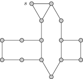
(a)

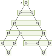
(b)

Figure 1: Example of a layering partition. A given graph $G$ LABEL:sub@fig:LayPartExG and the layering partition of $G$ generated when starting at vertex $s$ LABEL:sub@fig:LayPartExT. Example taken from [5].

For the remainder of this section, assume that we are given a graph $G=(V,E)$ and a layering partition $\mathcal{T}$ of $G$ for an arbitrary start vertex. We denote the largest diameter of all clusters of $\mathcal{T}$ as $\Delta$, i. e., $\Delta:=\max\big{\{}\,d_{G}(x,y)\mid\text{$x,y$ are in a cluster~{}$C$ of~{}$\mathcal{T}$}\,\big{\}}$. For two vertices $u$ and $v$ of $G$ contained in the clusters $C_{u}$ and $C_{v}$ of $\mathcal{T}$, respectively, we define $d_{\mathcal{T}}(u,v):=d_{\mathcal{T}}(C_{u},C_{v})$.

Lemma 1

For all vertices $u$ and $v$ of $G$, $d_{\mathcal{T}}(u,v)\leq d_{G}(u,v)\leq d_{\mathcal{T}}(u,v)+\Delta$.

Proof

Clearly, by construction of a layering partition, $d_{\mathcal{T}}(u,v)\leq d_{G}(u,v)$ for all vertices $u$ and $v$ of $G$.

Next, let $C_{u}$ and $C_{v}$ be the clusters containing $u$ and $v$, respectively. Note that $\mathcal{T}$ is a rooted tree. Let $C^{\prime}$ be the lowest common ancestor of $C_{u}$ and $C_{v}$. Therefore, $d_{\mathcal{T}}(u,v)=d_{\mathcal{T}}(u,C^{\prime})+d_{\mathcal{T}}(C^{\prime},v)$. By construction of a layering partition, $C^{\prime}$ contains a vertex $u^{\prime}$ and vertex $v^{\prime}$ such that $d_{G}(u,u^{\prime})=d_{\mathcal{T}}(u,u^{\prime})$ and $d_{G}(v,v^{\prime})=d_{\mathcal{T}}(v,v^{\prime})$. Since the diameter of each cluster is at most $\Delta$, $d_{G}(u,v)\leq d_{\mathcal{T}}(u,u^{\prime})+\Delta+d_{\mathcal{T}}(v,v^{\prime})=d_{\mathcal{T}}(u,v)+\Delta$.  $\square$

Theorem 3.1 below shows that we can use the layering partition $\mathcal{T}$ to compute an $(r+\Delta)$-dominating set for $G$ in linear time which is not larger than a minimum $r$-dominating set for $G$. This is done by finding a minimum $r$-dominating set of $\mathcal{T}$ where, for each cluster $C$ of $\mathcal{T}$, $r(C)$ is defined as $\min_{v\in C}r(v)$.

Theorem 3.1

Let $D$ be a minimum $r$-dominating set for a given graph $G$. An $(r+\Delta)$-dominating set $D^{\prime}$ for $G$ with $|D^{\prime}|\leq|D|$ can be computed in linear time.

Proof

First, create a layering partition $\mathcal{T}$ of $G$ and, for each cluster $C$ of $\mathcal{T}$, set $r(C):=\min_{v\in C}r(v)$. Second, find a minimum $r$-dominating set $\mathcal{S}$ for $\mathcal{T}$, i. e., a set $\mathcal{S}$ of clusters such that, for each cluster $C$ of $\mathcal{T}$, $d_{\mathcal{T}}(C,\mathcal{S})\leq r(C)$. Third, create a set $D^{\prime}$ by picking an arbitrary vertex of $G$ from each cluster in $\mathcal{S}$. All three steps can be performed in linear time, including the computation of $\mathcal{S}$ (see [3]).

Next, we show that $D^{\prime}$ is an $(r+\Delta)$-dominating set for $G$. By construction of $\mathcal{S}$, each cluster $C$ of $\mathcal{T}$ has distance at most $r(C)$ to $\mathcal{S}$ in $\mathcal{T}$. Thus, for each vertex $u$ of $G$, $\mathcal{S}$ contains a cluster $C_{\mathcal{S}}$ with $d_{\mathcal{T}}(u,C_{\mathcal{S}})\leq r(u)$. Additionally, by Lemma 1, $d_{G}(u,v)\leq r(u)+\Delta$ for any vertex $v\in C_{\mathcal{S}}$. Therefore, for any vertex $u$, $d_{G}(u,D^{\prime})\leq r(u)+\Delta$, i. e., $D^{\prime}$ is an $(r+\Delta)$-dominating set for $G$.

It remains to show that $|D^{\prime}|\leq|D|$. Let $\mathcal{D}$ be the set of clusters of $\mathcal{T}$ that contain a vertex of $D$. Because $D$ is an $r$-dominating set for $G$, it follows from Lemma 1 that $\mathcal{D}$ is an $r$-dominating set for $\mathcal{T}$. Clearly, since clusters are pairwise disjoint, $|\mathcal{D}|\leq|D|$. By minimality of $\mathcal{S}$, $|\mathcal{S}|\leq|\mathcal{D}|$ and, by construction of $D^{\prime}$, $|D^{\prime}|=|\mathcal{S}|$. Therefore, $|D^{\prime}|\leq|D|$.  $\square$

We now show how to construct a connected $(r+2\Delta)$-dominating set for $G$ using $\mathcal{T}$ in such a way that the set created is not larger than a minimum connected $r$-dominating set for $G$. For the remainder of this section, let $D_{r}$ be a minimum connected $r$-dominating set of $G$ and let, for each cluster $C$ of $\mathcal{T}$, $r(C)$ be defined as above. Additionally, we say that a subtree $T^{\prime}$ of some tree $T$ is an $r$-dominating subtree of $T$ if the nodes (clusters in case of a layering partition) of $T^{\prime}$ form a connected $r$-dominating set for $T$.

The first step of our approach is to construct a minimum $r$-dominating subtree $T_{r}$ of $\mathcal{T}$. Such a subtree $T_{r}$ can be computed in linear time [12]. Lemma 2 below shows that $T_{r}$ gives a lower bound for the cardinality of $D_{r}$.

Lemma 2

If $T_{r}$ contains more than one cluster, each connected $r$-dominating set of $G$ intersects all clusters of $T_{r}$. Therefore, $|T_{r}|\leq|D_{r}|$.

Proof

Let $D$ be an arbitrary connected $r$-dominating set of $G$. Assume that $T_{r}$ has a cluster $C$ such that $C\cap D=\emptyset$. Because $D$ is connected, the subtree of $\mathcal{T}$ induced by the clusters intersecting $D$ is connected, too. Thus, if $D$ intersects all leafs of $T_{r}$, then it intersects all clusters of $T_{r}$. Hence, we can assume, without loss of generality, that $C$ is a leaf of $T_{r}$. Because $T_{r}$ has at least two clusters and by minimality of $T_{r}$, $\mathcal{T}$ contains a cluster $C^{\prime}$ such that $d_{\mathcal{T}}(C^{\prime},C)=d_{\mathcal{T}}(C^{\prime},T_{r})=r(C^{\prime})$. Note that each path in $G$ from a vertex in $C^{\prime}$ to a vertex in $D$ intersects $C$. Therefore, by Lemma 1, there is a vertex $u\in C^{\prime}$ with $r(u)=d_{\mathcal{T}}(u,C)<d_{\mathcal{T}}(u,D)\leq d_{G}(u,D)$. That contradicts with $D$ being an $r$-dominating set.

Because any $r$-dominating set of $G$ intersects each cluster of $T_{r}$ and because these clusters are pairwise disjoint, it follows that $|T_{r}|\leq|D_{r}|$.  $\square$

As we show later in Corollary 1, each connected vertex set $S\subseteq V$ that intersects each cluster of $T_{r}$ gives an $(r+\Delta)$-dominating set for $G$. It follows from Lemma 2 that, if such a set $S$ has minimum cardinality, $|S|\leq|D_{r}|$. However, finding a minimum cardinality connected set intersecting each cluster of a layering partition (or of a subtree of it) is as hard as finding a minimum Steiner tree.

The main idea of our approach is to construct a minimum $(r+\delta)$-dominating subtree $T_{\delta}$ of $\mathcal{T}$ for some integer $\delta$. We then compute a small enough connected set $S_{\delta}$ that intersects all cluster of $T_{\delta}$. By trying different values of $\delta$, we eventually construct a connected set $S_{\delta}$ such that $|S_{\delta}|\leq|T_{r}|$ and, thus, $|S_{\delta}|\leq|D_{r}|$. Additionally, we show that $S_{\delta}$ is a connected $(r+2\Delta)$-dominating set of $G$.

For some non-negative integer $\delta$, let $T_{\delta}$ be a minimum $(r+\delta)$-dominating subtree of $\mathcal{T}$. Clearly, $T_{0}=T_{r}$. The following two lemmas set an upper bound for the maximum distance of a vertex of $G$ to a vertex in a cluster of $T_{\delta}$ and for the size of $T_{\delta}$ compared to the size of $T_{r}$.

Lemma 3

For each vertex $v$ of $G$, $d_{\mathcal{T}}(v,T_{\delta})\leq r(v)+\delta$.

Proof

Let $C_{v}$ be the cluster of $\mathcal{T}$ containing $v$ and let $C$ be the cluster of $T_{\delta}$ closest to $C_{v}$ in $\mathcal{T}$. By construction of $T_{\delta}$, $d_{\mathcal{T}}(v,C)=d_{\mathcal{T}}(C_{v},C)\leq r(C_{v})+\delta\leq r(v)+\delta$.  $\square$

Because the diameter of each cluster is at most $\Delta$, Lemma 1 and Lemma 3 imply the following.

Corollary 1

If a vertex set intersects all clusters of $T_{\delta}$, it is an $\big{(}r+(\delta+\Delta)\big{)}$-dominating set of $G$.

Lemma 4

$|T_{\delta}|\leq|T_{r}|-\delta\cdot\Lambda(T_{\delta})$.

Proof

First, consider the case when $T_{\delta}$ contains only one cluster, i. e., $|T_{\delta}|=1$. Then, $\Lambda(T_{\delta})=1$ and, thus, the statement clearly holds. Next, let $T_{\delta}$ contain more than one cluster, let $C_{u}$ be an arbitrary leaf of $T_{\delta}$, and let $C_{v}$ be a cluster of $T_{r}$ with maximum distance to $C_{u}$ such that $C_{u}$ is the only cluster on the shortest path from $C_{u}$ to $C_{v}$ in $T_{r}$, i. e., $C_{v}$ is not in $T_{\delta}$. Due to the minimality of $T_{\delta}$, $d_{T_{r}}(C_{u},C_{v})=\delta$. Thus, the shortest path from $C_{u}$ to $C_{v}$ in $T_{r}$ contains $\delta$ clusters (including $C_{v}$) which are not in $T_{\delta}$. Therefore, $|T_{\delta}|\leq|T_{r}|-\delta\cdot\Lambda(T_{\delta})$.  $\square$

Now that we have constructed and analysed $T_{\delta}$, we show how to construct $S_{\delta}$. First, we construct a set of shortest paths such that each cluster of $T_{\delta}$ is intersected by exactly one path. Second, we connect these paths with each other to from a connected set using an approach which is similar to Kruskal’s algorithm for minimum spanning trees.

Let $\mathcal{L}=\big{\{}C_{1},C_{2},\ldots,C_{\lambda}\big{\}}$ be the leaf clusters of $T_{\delta}$ (excluding the root) with either $\lambda=\Lambda(T_{\delta})-1$ if the root of $T_{\delta}$ is a leaf, or with $\lambda=\Lambda(T_{\delta})$ otherwise. We construct a set $\mathcal{P}=\big{\{}P_{1},P_{2},\ldots,P_{\lambda}\big{\}}$ of paths as follows. Initially, $\mathcal{P}$ is empty. For each cluster $C_{i}\in\mathcal{L}$, in turn, find the ancestor $C_{i}^{\prime}$ of $C_{i}$ which is closest to the root of $T_{\delta}$ and does not intersect any path in $\mathcal{P}$ yet. If we assume that the indices of the clusters in $\mathcal{L}$ represent the order in which they are processed, then $C_{1}^{\prime}$ is the root of $T_{\delta}$. Then, select an arbitrary vertex $v$ in $\mathcal{C}_{i}$ and find a shortest path $P_{i}$ in $G$ form $v$ to $C_{i}^{\prime}$. Add $P_{i}$ to $\mathcal{P}$ and continue with the next cluster in $\mathcal{L}$. Figure 2 gives an example.

Figure 2: Example for the set $\mathcal{P}$ for a subtree of a layering partition. Paths are shown in red. Each path $P_{i}$, with $1\leq i\leq 5$, starts in the leaf $C_{i}$ and ends in the cluster $C_{i}^{\prime}$. For $i=2$ and $i=5$, $P_{i}$ contains only one vertex.

Lemma 5

For each cluster $C$ of $T_{\delta}$, there is exactly one path $P_{i}\in\mathcal{P}$ intersecting $C$. Additionally, $C$ and $P_{i}$ share exactly one vertex, i. e., $|C\cap P_{i}|=1$.

Proof

Observe that, by construction of a layering partition, each vertex in a cluster $C$ is adjacent to some vertex in the parent cluster of $C$. Therefore, a shortest path $P$ in $G$ from $C$ to any of its ancestors $C^{\prime}$ only intersects clusters on the path from $C$ to $C^{\prime}$ in $\mathcal{T}$ and each cluster shares only one vertex with $P$. It remains to show that each cluster intersects exactly one path.

Without loss of generality, assume that the indices of clusters in $\mathcal{L}$ and paths in $\mathcal{P}$ represent the order in which they are processed and created, i. e., assume that the algorithms first creates $P_{1}$ which starts in $C_{1}$, then $P_{2}$ which starts in $C_{2}$, and so on. Additionally, let $\mathcal{L}_{i}=\{C_{1},C_{2},\ldots,C_{i}\}$ and $\mathcal{P}_{i}=\{P_{1},P_{2},\ldots,P_{i}\}$.

To proof that each cluster intersects exactly one path, we show by induction over $i$ that, if a cluster $C_{i}$ of $T_{\delta}$ satisfies the statement, then all ancestors of $C_{i}$ satisfy it, too. Thus, if $C_{\lambda}$ satisfies the statement, each cluster satisfies it.

First, consider $i=1$. Clearly, since $P_{1}$ is the first path, $P_{1}$ connects the leaf $C_{1}$ with the root of $T_{\delta}$ and no cluster intersects more than one path at this point. Therefore, the statement is true for $C_{1}$ and each of its ancestors.

Next, assume that $i>1$ and that the statement is true for each cluster in $\mathcal{L}_{i-1}$ and their respective ancestors. Then, the algorithm creates $P_{i}$ which connects the leaf $C_{i}$ with the cluster $C^{\prime}_{i}$. Assume that there is a cluster $C$ on the path from $C_{i}$ to $C_{i}^{\prime}$ in $\mathcal{T}$ such that $C$ intersects a path $P_{j}$ with $j<i$. Clearly, $C_{i}^{\prime}$ is an ancestor of $C$. Thus, by induction hypothesis, $C_{i}^{\prime}$ is also intersected by some path $P\neq P_{i}$. This contradicts with the way $C_{i}^{\prime}$ is selected by the algorithm. Therefore, each cluster on the path from $C_{i}$ to $C_{i}^{\prime}$ in $\mathcal{T}$ only intersects $P_{i}$ and $P_{i}$ does not intersect any other clusters.

Because $i>1$, $C^{\prime}_{i}$ has a parent cluster $C^{\prime\prime}$ in $T_{\delta}$ that is intersected by a path $P_{j}$ with $j<i$. By induction hypothesis, each ancestor of $C^{\prime\prime}$ is intersected by a path in $\mathcal{P}_{i-1}$. Therefore, each ancestor of $C_{i}$ is intersected by exactly one path in $\mathcal{P}_{i}$.  $\square$

Next, we use the paths in $\mathcal{P}$ to create the set $S_{\delta}$. As first step, let $S_{\delta}:=\bigcup_{P_{i}\in\mathcal{P}}P_{i}$. Later, we add more vertices into $S_{\delta}$ to ensure it is a connected set.

Now, create a partition $\mathcal{V}=\big{\{}V_{1},V_{2},\ldots,V_{\lambda}\big{\}}$ of $V$ such that, for each $i$, $P_{i}\subseteq V_{i}$, $V_{i}$ is connected, and $d_{G}(v,P_{i})=\min_{P\in\mathcal{P}}d_{G}(v,P)$ for each vertex $v\in V_{i}$. That is, $V_{i}$ contains the vertices of $G$ which are not more distant to $P_{i}$ in $G$ than to any other path in $\mathcal{P}$. Additionally, for each vertex $v\in V$, set $P(v):=P_{i}$ if and only if $v\in V_{i}$ (i. e., $P(v)$ is the path in $\mathcal{P}$ which is closest to $v$) and set $d(v):=d_{G}\big{(}v,P(v)\big{)}$. Such a partition as well as $P(v)$ and $d(v)$ can be computed by performing a BFS on $G$ starting at all paths $P_{i}\in\mathcal{P}$ simultaneously. Later, the BFS also allows us to easily determine the shortest path from $v$ to $P(v)$ for each vertex $v$.

To manage the subsets of $\mathcal{V}$, we use a Union-Find data structure such that, for two vertices $u$ and $v$, $\mathrm{Find}(u)=\mathrm{Find}(v)$ if and only if $u$ and $v$ are in the same set of $\mathcal{V}$. A Union-Find data structure additionally allows us to easily join two set of $\mathcal{V}$ into one by performing a single $\mathrm{Union}$ operation. Note that, whenever we join two sets of $\mathcal{V}$ into one, $P(v)$ and $d(v)$ remain unchanged for each vertex $v$.

Next, create an edge set $E^{\prime}=\{\,uv\mid\mathrm{Find}(u)\neq\mathrm{Find}(v)\,\}$, i. e., the set of edges $uv$ such that $u$ and $v$ are in different sets of $\mathcal{V}$. Sort $E^{\prime}$ in such a way that an edge $uv$ precedes an edge $xy$ only if $d(u)+d(v)\leq d(x)+d(y)$.

The last step to create $S_{\delta}$ is similar to Kruskal’s minimum spanning tree algorithm. Iterate over the edges in $E^{\prime}$ in increasing order. If, for an edge $uv$, $\mathrm{Find}(u)\neq\mathrm{Find}(v)$, i. e., if $u$ and $v$ are in different sets of $\mathcal{V}$, then join these sets into one by performing $\mathrm{Union}(u,v)$, add the vertices on the shortest path from $u$ to $P(u)$ to $S_{\delta}$, and add the vertices on the shortest path from $v$ to $P(v)$ to $S_{\delta}$. Repeat this, until $\mathcal{V}$ contains only one set, i. e., until $\mathcal{V}=\{V\}$.

Algorithm 1 below summarises the steps to create a set $S_{\delta}$ for a given subtree of a layering partition subtree $T_{\delta}$.

1

Input: A graph $G=(V,E)$ and a subtree $T_{\delta}$ of some layering partition of $G$.

2

Output: A connected set $S_{\delta}\subseteq V$ that intersects each cluster of $T_{\delta}$ and contains at most $|T_{\delta}|+\big{(}\Lambda(T_{\delta})-1\big{)}\cdot\Delta$ vertices.

3

4Let $\mathcal{L}=\big{\{}C_{1},C_{2},\ldots,C_{\lambda}\big{\}}$ be the set of clusters excluding the root that are leaves of $T_{\delta}$.

5Create an empty set $\mathcal{P}$.

6foreach cluster $C_{i}\in\mathcal{L}$  do

7      Select an arbitrary vertex $v\in C_{i}$.

8      Find the highest ancestor $C_{i}^{\prime}$ of $C_{i}$ (i. e., the ancestor which is closest to the root of $T_{\delta}$) that is not flagged.

9      Find a shortest path $P_{i}$ from $v$ to an ancestor of $v$ in $C_{i}^{\prime}$ (i. e., a shortest path from $C_{i}$ to $C_{i}^{\prime}$ in $G$ that contains exactly one vertex of each cluster of the corresponding path in $T_{\delta}$).

10      Add $P_{i}$ to $\mathcal{P}$.

11      Flag each cluster intersected by $P_{i}$.

12

13Create a set $S_{\delta}:=\bigcup_{P_{i}\in\mathcal{P}}P_{i}$.

14Perform a BFS on $G$ starting at all paths $P_{i}\in\mathcal{P}$ simultaneously. This results in a partition $\mathcal{V}=\big{\{}V_{1},V_{2},\ldots,V_{\lambda}\big{\}}$ of $V$ with $P_{i}\subseteq V_{i}$ for each $P_{i}\in\mathcal{P}$. For each vertex $v$, set $P(v):=P_{i}$ if and only if $v\in V_{i}$ and let $d(v):=d_{G}(v,P(v))$.

15Create a Union-Find data structure and add all vertices of $G$ such that $\mathrm{Find}(v)=i$ if and only if $v\in V_{i}$.

16Determine the edge set $E^{\prime}=\{\,uv\mid\mathrm{Find}(u)\neq\mathrm{Find}(v)\,\}$.

17Sort $E^{\prime}$ such that $uv\leq xy$ if and only if $d(u)+d(v)\leq d(x)+d(y)$. Let $\langle e_{1},e_{2},\ldots,e_{|E^{\prime}|}\rangle$ be the resulting sequence.

18for $i:=1$ to $|E^{\prime}|$  do

19      Let $uv=e_{i}$.

20      if $\mathrm{Find}(u)\neq\mathrm{Find}(v)$  then

21            Add the shortest path from $u$ to $P(u)$ to $S_{\delta}$.

22            Add the shortest path from $v$ to $P(v)$ to $S_{\delta}$.

23            $\mathrm{Union}(u,v)$

24      

25

Output $S_{\delta}$.

Algorithm 1 Computes a connected vertex set that intersects each cluster of a given layering partition.

Lemma 6

For a given graph $G$ and a given subtree $T_{\delta}$ of some layering partition of $G$, Algorithm 1 constructs, in $\mathcal{O}\big{(}m\,\alpha(n)\big{)}$ time, a connected set $S_{\delta}$ with $|S_{\delta}|\leq|T_{\delta}|+\Delta\cdot\Lambda(T_{\delta})$ which intersects each cluster of $T_{\delta}$.

Proof (Correctness)

First, we show that $S_{\delta}$ is connected at the end of the algorithm. To do so, we show by induction that, at any time, $S_{\delta}\cap V^{\prime}$ is a connected set for each set $V^{\prime}\in\mathcal{V}$. Clearly, when $\mathcal{V}$ is created, for each set $V_{i}\in\mathcal{V}$, $S_{\delta}\cap V_{i}=P_{i}$. Now, assume that the algorithm joins the set $V_{u}$ and $V_{v}$ in $\mathcal{V}$ into one set based on the edge $uv$ with $u\in V_{u}$ and $v\in V_{v}$. Let $S_{u}=S_{\delta}\cap V_{u}$ and $S_{v}=S_{\delta}\cap V_{v}$. Note that $P(u)\subseteq S_{u}$ and $P(v)\subseteq S_{v}$. The algorithm now adds all vertices to $S_{\delta}$ which are on a path from $P(u)$ to $P(v)$. Therefore, $S_{\delta}\cap(V_{u}\cup V_{v})$ is a connected set. Because $\mathcal{V}=\{V\}$ at the end of the algorithm, $S_{\delta}$ is connected eventually. Additionally, since $P_{i}\subseteq S_{\delta}$ for each $P_{i}\in\mathcal{P}$, it follows that $S_{\delta}$ intersects each cluster of $T_{\delta}$.

Next, we show that the cardinality of $S_{\delta}$ is at most $|T_{\delta}|+\Delta\cdot\Lambda(T_{\delta})$. When first created, the set $S_{\delta}$ contains all vertices of all paths in $\mathcal{P}$. Therefore, by Lemma 5, $|S_{\delta}|=\sum_{P_{i}\in\mathcal{P}}|P_{i}|=|T_{\delta}|$. Then, each time two sets of $\mathcal{V}$ are joined into one set based on an edge $uv$, $S_{\delta}$ is extended by the vertices on the shortest paths from $u$ to $P(u)$ and from $v$ to $P(v)$. Therefore, the size of $S_{\delta}$ increases by $d(u)+d(v)$, i. e., $|S_{\delta}|:=|S_{\delta}|+d(u)+d(v)$. Let $X$ denote the set of all edges used to join two sets of $\mathcal{V}$ into one at some point during the algorithm. Note that $|X|=|\mathcal{P}|-1\leq\Lambda(T_{\delta})$. Therefore, at the end of the algorithm,

$$|S_{\delta}|=\sum_{\mathclap{P_{i}\in\mathcal{P}}}|P_{i}|+\sum_{\mathclap{uv\in X}}\big{(}d(u)+d(v)\big{)}\leq|T_{\delta}|+\Lambda(T_{\delta})\cdot\max_{\mathclap{uv\in X}}\big{(}d(u)+d(v)\big{)}.$$

Claim

For each edge $uv\in X$, $d(u)+d(v)\leq\Delta$.

Proof (Claim)

To represent the relations between paths in $\mathcal{P}$ and vertex sets in $\mathcal{V}$, we define a function $f\colon\mathcal{P}\rightarrow\mathcal{V}$ such that $f(P_{i})=V_{j}$ if and only if $P_{i}\subseteq V_{j}$. Directly after constructing $\mathcal{V}$, $f$ is a bijection with $f(P_{i})=V_{i}$. At the end of the algorithm, after all sets of $\mathcal{V}$ are joined into one, $f(P_{i})=V$ for all $P_{i}\in\mathcal{P}$.

Recall the construction of $\mathcal{P}$ and assume that the indices of the paths in $\mathcal{P}$ represent the order in which they are created. Assume that $i>1$. By construction, the path $P_{i}\in\mathcal{P}$ connects the leaf $C_{i}$ with the cluster $C^{\prime}_{i}$ in $T_{\delta}$. Because $i>1$, $C^{\prime}_{i}$ has a parent cluster in $T_{\delta}$ that is intersected by a path $P_{j}\in\mathcal{P}$ with $j<i$. We define $P_{j}$ as the parent of $P_{i}$. By Lemma 5, this parent $P_{j}$ is unique for each $P_{i}\in\mathcal{P}$ with $i>1$. Based on this relation between paths in $\mathcal{P}$, we can construct a rooted tree $\mathbb{T}$ with the node set $\{\,x_{i}\mid P_{i}\in\mathcal{P}\,\}$ such that each node $x_{i}$ represents the path $P_{i}$ and $x_{j}$ is the parent of $x_{i}$ if and only if $P_{j}$ is the parent of $P_{i}$.

Because each node of $\mathbb{T}$ represents a path in $\mathcal{P}$, $f$ defines a colouring for the nodes of $\mathbb{T}$ such that $x_{i}$ and $x_{j}$ have different colours if and only if $f(P_{i})\neq f(P_{j})$. As long as $|\mathcal{V}|>1$, $\mathbb{T}$ contains two adjacent nodes with different colours. Let $x_{i}$ and $x_{j}$ be these nodes with $j<i$ and let $P_{i}$ and $P_{j}$ be the corresponding paths in $\mathcal{P}$. Note that $x_{j}$ is the parent of $x_{i}$ in $\mathbb{T}$ and, hence, $P_{j}$ is the parent of $P_{i}$. Therefore, $P_{i}$ ends in a cluster $C^{\prime}_{i}$ which has a parent cluster $C$ that intersects $P_{j}$. By properties of layering partitions, it follows that $d_{G}(P_{i},P_{j})\leq\Delta+1$. Recall that, by construction, $d(v)=\min_{P\in\mathcal{P}}d_{G}(v,P)$ for each vertex $v$. Thus, for each edge $uv$ on a shortest path from $P_{i}$ to $P_{j}$ in $G$ (with $u$ being closer to $P_{i}$ than to $P_{j}$), $d(u)+d(v)\leq d_{G}(u,P_{i})+d_{G}(v,P_{j})\leq\Delta$. Therefore, because $f(P_{i})\neq f(P_{j})$, there is an edge $uv$ on a shortest path from $P_{i}$ to $P_{j}$ such that $f\big{(}P(u)\big{)}\neq f\big{(}P(v)\big{)}$ and $d(u)+d(v)\leq\Delta$.  $\lozenge$

From the claim above, it follows that, as long as $\mathcal{V}$ contains multiple sets, there is an edge $uv\in E^{\prime}$ such that $d(u)+d(v)\leq\Delta$ and $\mathrm{Find}(u)\neq\mathrm{Find}(v)$. Therefore, $\max_{uv\in X}\big{(}d(u)+d(v)\big{)}\leq\Delta$ and $|S_{\delta}|\leq|T_{\delta}|+\big{(}\Lambda(T_{\delta})-1\big{)}\cdot\Delta$.  $\square$

Proof (Complexity)

First, the algorithm computes $\mathcal{P}$ (line 1 to line 1). If the parent of each vertex from the original BFS that was used to construct $\mathcal{T}$ is still known, $\mathcal{P}$ can be constructed in $\mathcal{O}(n)$ total time. After picking a vertex $v$ in $C_{i}$, simply follow the parent pointers until a vertex in $C_{i}^{\prime}$ is reached. Computing $\mathcal{V}$ as well as $P(v)$ and $d(v)$ for each vertex $v$ of $G$ (line 1) can be done with single BFS and, thus, requires at most $\mathcal{O}(n+m)$ time.

Recall that, for a Union-Find data structure storing $n$ elements, each operation requires at most $\mathcal{O}\big{(}\alpha(n)\big{)}$ amortised time. Therefore, initialising such a data structure to store all vertices (line 1) and computing $E^{\prime}$ (line 1) requires at most $\mathcal{O}\big{(}m\,\alpha(n)\big{)}$ time. Note that, for each vertex $v$, $d(v)\leq|V|$. Thus, sorting $E^{\prime}$ (line 1) can be done in linear time using counting sort. When iterating over $E^{\prime}$ (line 1 to line 1), for each edge $uv\in E^{\prime}$, the $\mathrm{Find}$-operation is called twice and the $\mathrm{Union}$-operation is called at most once. Thus, the total runtime for all these operations is at most $\mathcal{O}\big{(}m\,\alpha(n)\big{)}$.

Let $P_{u}=\{u,\ldots,x,y,\ldots,p\}$ be the shortest path in $G$ from a vertex $u$ to $P(u)$. Assume that $y$ has been added to $S_{\delta}$ in a previous iteration. Thus, $\{y,\ldots,p\}\subseteq S_{\delta}$ and, when adding $P_{u}$ to $S_{\delta}$, the algorithm only needs to add $\{u,\ldots,x\}$. Therefore, by using a simple binary flag to determine if a vertex is contained in $S_{\delta}$, constructing $S_{\delta}$ (line 1, line 1, and line 1) requires at most $\mathcal{O}(n)$ time.

In total, Algorithm 1 runs in $\mathcal{O}\big{(}m\,\alpha(n)\big{)}$ time.  $\square$

Because, for each integer $\delta\geq 0$, $|S_{\delta}|\leq|T_{\delta}|+\Delta\cdot\Lambda(T_{\delta})$ (Lemma 6) and $|T_{\delta}|\leq|T_{r}|-\delta\cdot\Lambda(T_{\delta})$ (Lemma 4), we have the following.

Corollary 2

For each $\delta\geq\Delta$, $|S_{\delta}|\leq|T_{r}|$ and, thus, $|S_{\delta}|\leq|D_{r}|$.

To the best of our knowledge, there is no algorithm known that computes $\Delta$ in less than $\mathcal{O}(nm)$ time. Additionally, under reasonable assumptions, computing the diameter or radius of a general graph requires $\Omega\big{(}n^{2}\big{)}$ time [1]. We conjecture that the runtime for computing $\Delta$ for a given graph has a similar lower bound.

To avoid the runtime required for computing $\Delta$, we use the following approach shown in Algorithm 2 below. First, compute a layering partition $\mathcal{T}$ and the subtree $T_{r}$. Second, for a certain value of $\delta$, compute $T_{\delta}$ and perform Algorithm 1 on it. If the resulting set $S_{\delta}$ is larger than $T_{r}$ (i. e., $|S_{\delta}|>|T_{r}|$), increase $\delta$; otherwise, if $|S_{\delta}|\leq|T_{r}|$, decrease $\delta$. Repeat the second step with the new value of $\delta$.

One strategy to select values for $\delta$ is a classical binary search over the number of vertices of $G$. In this case, Algorithm 1 is called up-to $\mathcal{O}(\log n)$ times. Empirical analysis [2], however, have shown that $\Delta$ is usually very small. Therefore, we use a so-called one-sided binary search.

Consider a sorted sequence $\langle x_{1},x_{2},\ldots,x_{n}\rangle$ in which we search for a value $x_{p}$. We say the value $x_{i}$ is at position $i$. For a one-sided binary search, instead of starting in the middle at position $n/2$, we start at position $1$. We then processes position $2$, then position $4$, then position $8$, and so on until we reach position $j=2^{i}$ and, next, position $k=2^{i+1}$ with $x_{j}<x_{p}\leq x_{k}$. Then, we perform a classical binary search on the sequence $\langle x_{j+1},\ldots,x_{k}\rangle$. Note that, because $x_{j}<x_{p}\leq x_{k}$, $2^{i}<p\leq 2^{i+1}$ and, hence, $j<p\leq k<2p$. Therefore, a one-sided binary search requires at most $\mathcal{O}(\log p)$ iterations to find $x_{p}$.

Because of Corollary 2, using a one-sided binary search allows us to find a value $\delta\leq\Delta$ for which $|S_{\delta}|\leq|T_{r}|$ by calling Algorithm 1 at most $\mathcal{O}(\log\Delta)$ times. Algorithm 2 below implements this approach.

1

Input: A graph $G=(V,E)$ and a function $r\colon V\rightarrow\mathbb{N}$.

2

Output: A connected $(r+2\Delta)$-dominating set $D$ for $G$ with $|D|\leq|D_{r}|$.

3

4Create a layering partition $\mathcal{T}$ of $G$.

5For each cluster $C$ of $\mathcal{T}$, set $r(C):=\min_{v\in C}r(v)$.

6Compute a minimum $r$-dominating subtree $T_{r}$ for $\mathcal{T}$ (see [12]).

7One-Sided Binary Search over $\delta$, starting with $\delta=0$  

8      Create a minimum $\delta$-dominating subtree $T_{\delta}$ of $T_{r}$ (i. e., $T_{\delta}$ is a minimum $(r+\delta)$-dominating subtree for $\mathcal{T}$).

9      Run Algorithm 1 on $T_{\delta}$ and let the set $S_{\delta}$ be the corresponding output.

10      if $|S_{\delta}|\leq|T_{r}|$ then

11            Decrease $\delta$.

12      else

13            Increase $\delta$.

14      

15

Output $S_{\delta}$ with the smallest $\delta$ for which $|S_{\delta}|\leq|T_{r}|$.

Algorithm 2 Computes a connected $(r+2\Delta)$-dominating set for a given graph $G$.

Theorem 3.2

For a given graph $G$, Algorithm 2 computes a connected $(r+2\Delta)$-dominating set $D$ with $|D|\leq|D_{r}|$ in $\mathcal{O}\big{(}m\,\alpha(n)\log\Delta\big{)}$ time.

Proof

Clearly, the set $D$ is connected because $D=S_{\delta}$ for some $\delta$ and, by Lemma 6, the set $S_{\delta}$ is connected. By Corollary 2, for each $\delta\geq\Delta$, $|S_{\delta}|\leq|T_{r}|$. Thus, for each $\delta\geq\Delta$, the binary search decreases $\delta$ and, eventually, finds some $\delta$ such that $\delta\leq\Delta$ and $|S_{\delta}|\leq|T_{r}|$. Therefore, the algorithm finds a set $D$ with $|D|\leq|D_{r}|$. Note that, because $D=S_{\delta}$ for some $\delta\leq\Delta$ and because $S_{\delta}$ intersects each cluster of $T_{\delta}$ (Lemma 6), it follows from Lemma 3 that, for each vertex $v$ of $G$, $d_{\mathcal{T}}(v,D)\leq r(v)+\Delta$ and, by Lemma 1, $d_{G}(v,D)\leq r(v)+2\Delta$. Thus, $D$ is an $(r+2\Delta)$-dominating set for $G$.

Creating a layering partition for a given graph and computing a minimum connected $r$-dominating set of a tree can be done in linear time [12]. The one-sided binary search over $\delta$ has at most $\mathcal{O}(\log\Delta)$ iterations. Each iteration of the binary search requires at most linear time to compute $T_{\delta}$, $\mathcal{O}\big{(}m\,\alpha(n)\big{)}$ time to compute $S_{\delta}$ (Lemma 6), and constant time to decide whether to increase or decrease $\delta$. Therefore, Algorithm 2 runs in $\mathcal{O}\big{(}m\,\alpha(n)\log\Delta\big{)}$ total time.  $\square$

4 Using a Tree-Decomposition

Theorem 3.1 and Theorem 3.2 respectively show how to compute an $(r+\Delta)$-dominating set in linear time and a connected $(r+2\Delta)$-dominating set in $\mathcal{O}\big{(}m\,\alpha(n)\log\Delta\big{)}$ time. It is known that the maximum diameter $\Delta$ of clusters of any layering partition of a graph approximates the tree-breadth and tree-length of this graph. Indeed, for a graph $G$ with $\operatorname{tl}(G)=\lambda$, $\Delta\leq 3\lambda$ [10].

Corollary 3

Let $D$ be a minimum $r$-dominating set for a given graph $G$ with $\operatorname{tl}(G)=\lambda$. An $(r+3\lambda)$-dominating set $D^{\prime}$ for $G$ with $|D^{\prime}|\leq|D|$ can be computed in linear time.

Corollary 4

Let $D$ be a minimum connected $r$-dominating set for a given graph $G$ with $\operatorname{tl}(G)=\lambda$. A connected $(r+6\lambda)$-dominating set $D^{\prime}$ for $G$ with $|D^{\prime}|\leq|D|$ can be computed in $\mathcal{O}\big{(}m\,\alpha(n)\log\lambda\big{)}$ time.

In this section, we consider the case when we are given a tree-decomposition with breadth $\rho$ and length $\lambda$. We present algorithms to compute an $(r+\rho)$-dominating set as well as a connected $\big{(}r+\min(3\lambda,5\rho)\big{)}$-dominating set in $\mathcal{O}(nm)$ time.

For the remainder of this section, assume that we are given a graph $G=(V,E)$ and a tree-decomposition $\mathcal{T}$ of $G$ with breadth $\rho$ and length $\lambda$. We assume that $\rho$ and $\lambda$ are known and that, for each bag $B$ of $\mathcal{T}$, we know a vertex $c(B)$ with $B\subseteq N_{G}^{\rho}[c(B)]$. Let $\mathcal{T}$ be minimal, i. e., $B\nsubseteq B^{\prime}$ for any two bags $B$ and $B^{\prime}$. Thus, the number of bags is not exceeding the number vertices of $G$. Additionally, let each vertex of $G$ store a list of bags containing it and let each bag of $T$ store a list of vertices it contains. One can see this as a bipartite graph where one subset of vertices are the vertices of $G$ and the other subset are the bags of $\mathcal{T}$. Therefore, the total input size is in $\mathcal{O}(n+m+M)$ where $M\leq n^{2}$ is the sum of the cardinality of all bags of $\mathcal{T}$.

4.1 Preprocessing

Before approaching the (Connected) $r$-Domination problem, we compute a subtree $\mathcal{T}^{\prime}$ of $\mathcal{T}$ such that, for each vertex $v$ of $G$, $\mathcal{T}^{\prime}$ contains a bag $B$ with $d_{G}(v,B)\leq r(v)$. We call such a (not necessarily minimal) subtree an $r$-covering subtree of $\mathcal{T}$.

Let $T_{r}$ be a minimum $r$-covering subtree of $\mathcal{T}$. We do not know how to compute $T_{r}$ directly. However, if we are given a bag $B$ of $\mathcal{T}$, we can compute the smallest $r$-covering subtree $T_{B}$ which contains $B$. Then, we can identify a bag $B^{\prime}$ in $T_{B}$ for which we know it is a bag of $T_{r}$. Thus, we can compute $T_{r}$ by computing the smallest $r$-covering subtree which contains $B^{\prime}$.

The idea for computing $T_{B}$ is to determine, for each vertex $v$ of $G$, the bag $B_{v}$ of $\mathcal{T}$ for which $d_{G}(v,B_{v})\leq r(v)$ and which is closet to $B$. Then, let $T_{B}$ be the smallest tree that contains all these bags $B_{v}$. Algorithm 3 below implements this approach.

Additionally to computing the tree $T_{B}$, we make it a rooted tree with $B$ as the root, give each vertex $v$ a pointer $\beta(v)$ to a bag of $T_{B}$, and give each bag $B^{\prime}$ a counter $\sigma(B^{\prime})$. The pointer $\beta(v)$ identifies the bag $B_{v}$ which is closest to $B$ in $T_{B}$ and intersects the $r$-neighbourhood of $v$. The counter $\sigma(B^{\prime})$ states the number of vertices $v$ with $\beta(v)=B^{\prime}$. Even though setting $\beta$ and $\sigma$ as well as rooting the tree are not necessary for computing $T_{B}$, we use it when computing an $(r+\rho)$-dominating set later.

1

2Make $\mathcal{T}$ a rooted tree with the bag $B$ as the root.

3Create a set $\mathcal{B}$ of bags and initialise it with $\mathcal{B}:=\{B\}$.

4For each bag $B^{\prime}$ of $\mathcal{T}$, set $\sigma(B^{\prime}):=0$ and determine $d_{\mathcal{T}}(B^{\prime},B)$.

5For each vertex $u$, determine the bag $B(u)$ which contains $u$ and has minimal distance to $B$.

6foreach $u\in V$  do

7      Determine a vertex $v$ such that $d_{G}(u,v)\leq r(u)$ and $d_{\mathcal{T}}\big{(}B(v),B\big{)}$ is minimal and let $B_{u}:=B(v)$.

8      Add $B_{u}$ to $\mathcal{B}$, set $\beta(u):=B_{u}$, and increase $\sigma(B_{u})$ by $1$.

9

Output the smallest subtree $T_{B}$ of $\mathcal{T}$ that contains all bags in $\mathcal{B}$.

Algorithm 3 Computes the smallest $r$-covering subtree $T_{B}$ of a given tree-decomposition $\mathcal{T}$ that contains a given bag $B$ of $\mathcal{T}$.

Lemma 7

For a given tree-decomposition $\mathcal{T}$ and a given bag $B$ of $\mathcal{T}$, Algorithm 3 computes an $r$-covering subtree $T_{B}$ in $\mathcal{O}(nm)$ time such that $T_{B}$ contains $B$ and has a minimal number of bags.

Proof (Correctness)

Note that, by construction of the set $\mathcal{B}$ (line 3 to line 3), $\mathcal{B}$ contains a bag $B_{u}$ for each vertex $u$ of $G$ such that $d_{G}(u,B_{u})\leq r(u)$. Thus, each subtree of $\mathcal{T}$ which contains all bags of $\mathcal{B}$ is an $r$-covering subtree. To show the correctness of the algorithm, it remains to show that the smallest $r$-covering subtree of $\mathcal{T}$ which contains $B$ has to contain each bag from the set $\mathcal{B}$. Then, the subtree $T_{B}$ constructed in line 3 is the desired subtree.

By properties of tree-decompositions, the set of bags which intersect the $r$-neighbourhood of some vertex $u$ induces a subtree $T_{u}$ of $\mathcal{T}$. That is, $T_{u}$ contains exactly the bags $B^{\prime}$ with $d_{G}(u,B^{\prime})\leq r(u)$. Note that $\mathcal{T}$ is a rooted tree with $B$ as the root. Clearly, the bag $B_{u}\in\mathcal{B}$ (determined in line 3) is the root of $T_{u}$ since it is the bag closest to $B$. Hence, each bag $B^{\prime}$ with $d_{G}(u,B^{\prime})\leq r(u)$ is a descendant of $B_{u}$. Therefore, if a subtree of $\mathcal{T}$ contains $B$ and does not contain $B_{u}$, then it also cannot contain any descendant of $B_{u}$ and, thus, contains no bag intersecting the $r$-neighbourhood of $u$.  $\square$

Proof (Complexity)

Recall that $\mathcal{T}$ has at most $n$ bags and that the sum of the cardinality of all bags of $\mathcal{T}$ is $M\leq n^{2}$. Thus, line 3 and line 3 require at most $\mathcal{O}(M)$ time. Using a BFS, it takes at most $\mathcal{O}(m)$ time, for a given vertex $u$, to determine a vertex $v$ such that $d_{G}(u,v)\leq r(u)$ and $d_{\mathcal{T}}\big{(}B(v),B\big{)}$ is minimal (line 3). Therefore, the loop starting in line 3 and, thus, Algorithm 3 run in at most $\mathcal{O}(nm)$ total time.  $\square$

Lemma 8 and Lemma 9 below show that each leaf $B^{\prime}\neq B$ of $T_{B}$ is a bag of a minimum $r$-covering subtree $T_{r}$ of $\mathcal{T}$. Note that both lemmas only apply if $T_{B}$ has at least two bags. If $T_{B}$ contains only one bag, it is clearly a minimum $r$-covering subtree.

Lemma 8

For each leaf $B^{\prime}\neq B$ of $T_{B}$, there is a vertex $v$ in $G$ such that $B^{\prime}$ is the only bag of $T_{B}$ with $d_{G}(v,B^{\prime})\leq r(v)$.

Proof

Assume that Lemma 8 is false. Then, there is a leaf $B^{\prime}$ such that, for each vertex $v$ with $d_{G}(v,B^{\prime})\leq r(v)$, $T_{B}$ contains a bag $B^{\prime\prime}\neq B^{\prime}$ with $d_{G}(v,B^{\prime\prime})\leq r(v)$. Thus, for each vertex $v$, the $r$-neighbourhood of $v$ is intersected by a bag of the tree-decomposition $T_{B}-B^{\prime}$. This contradicts with the minimality of $T_{B}$.  $\square$

Lemma 9

For each leaf $B^{\prime}\neq B$ of $T_{B}$, there is a minimum $r$-covering subtree $T_{r}$ of $\mathcal{T}$ which contains $B^{\prime}$.

Proof

Assume that $T_{r}$ is a minimum $r$-covering subtree which does not contain $B^{\prime}$. Because of Lemma 8, there is a vertex $v$ of $G$ such that $B^{\prime}$ is the only bag of $T_{B}$ which intersects the $r$-neighbourhood of $v$. Therefore, $T_{r}$ contains only bags which are descendants of $B^{\prime}$. Partition the vertices of $G$ into the sets $V^{\uparrow}$ and $V^{\downarrow}$ such that $V^{\downarrow}$ contains the vertices of $G$ which are contained in $B^{\prime}$ or in a descendant of $B^{\prime}$. Because $T_{r}$ is an $r$-covering subtree and because $T_{r}$ only contains descendants of $B^{\prime}$, it follows from properties of tree-decompositions that, for each vertex $v\in V^{\uparrow}$, there is a path of length at most $r(v)$ from $v$ to a bag of $T_{r}$ passing through $B^{\prime}$ and, thus, $d_{G}(v,B^{\prime})\leq r(v)$. Similarly, since $T_{B}$ is an $r$-covering subtree, it follows that, for each vertex $v\in V^{\downarrow}$, $d_{G}(v,B^{\prime})\leq r(v)$. Therefore, for each vertex $v$ of $G$, $d_{G}(v,B^{\prime})\leq r(v)$ and, thus, $B^{\prime}$ induces an $r$-covering subtree $T_{r}$ of $\mathcal{T}$ with $|T_{r}|=1$.  $\square$

Algorithm 4 below uses Lemma 9 to compute a minimum $r$-covering subtree $T_{r}$ of $\mathcal{T}$.

1

2Pick an arbitrary bag $B$ of $\mathcal{T}$.

3Determine the subtree $T_{B}$ of $\mathcal{T}$ using Algorithm 3.

4if $|T_{B}|=1$  then

5      Output $T_{r}:=T_{B}$.

6else

7      Select an arbitrary leaf $B^{\prime}\neq B$ of $T_{B}$.

8      Determine the subtree $T_{B^{\prime}}$ of $\mathcal{T}$ using Algorithm 3.

9      Output $T_{r}:=T_{B^{\prime}}$.

Algorithm 4 Computes a minimum $r$-covering subtree $T_{r}$ of a given tree-decomposition $\mathcal{T}$.

Lemma 10

Algorithm 4 computes a minimum $r$-covering subtree $T_{r}$ of $\mathcal{T}$ in $\mathcal{O}(nm)$ time.

Proof

Algorithm 4 first picks an arbitrary bag $B$ and then uses Algorithm 3 to compute the smallest $r$-covering subtree $T_{B}$ of $\mathcal{T}$ which contains $B$. By Lemma 9, for each leaf $B^{\prime}$ of $T_{B}$, there is a minimum $r$-covering subtree $T_{r}$ which contains $B^{\prime}$. Thus, performing Algorithm 3 again with $B^{\prime}$ as input creates such a subtree $T_{r}$.

Clearly, with exception of calling Algorithm 3, all steps of Algorithm 4 require only constant time. Because Algorithm 3 requires at most $\mathcal{O}(nm)$ time (see Lemma 7) and is called at most two times, Algorithm 4 runs in at most $\mathcal{O}(nm)$ total time.  $\square$

Algorithm 4 computes $T_{r}$ by, first, computing $T_{B}$ for some bag $B$ and, second, computing $T_{B^{\prime}}=T_{r}$ for some leaf $B^{\prime}$ of $T_{B}$. Note that, because both trees are computed using Algorithm 3, Lemma 8 applies to $T_{B}$ and $T_{B^{\prime}}$. Therefore, we can slightly generalise Lemma 8 as follows.

Corollary 5

For each leaf $B$ of $T_{r}$, there is a vertex $v$ in $G$ such that $B$ is the only bag of $T_{r}$ with $d_{G}(v,B)\leq r(v)$.

4.2 $r$-Domination

In this subsection, we use the minimum $r$-covering subtree $T_{r}$ to determine an $(r+\rho)$-dominating set $S$ in $\mathcal{O}(nm)$ time using the following approach. First, compute $T_{r}$. Second, pick a leaf $B$ of $T_{r}$. If there is a vertex $v$ such that $v$ is not dominated and $B$ is the only bag intersecting the $r$-neighbourhood of $v$, then add the center of $B$ into $S$, flag all vertices $u$ with $d_{G}(u,B)\leq r(u)$ as dominated, and remove $B$ from $T_{r}$. Repeat the second step until $T_{r}$ contains no more bags and each vertex is flagged as dominated. Algorithm 5 below implements this approach. Note that, instead of removing bags from $T_{r}$, we use a reversed BFS-order of the bags to ensure the algorithm processes bags in the correct order.

1

2Compute a minimum $r$-covering subtree $T_{r}$ of $\mathcal{T}$ using Algorithm 4.

3Give each vertex $v$ a binary flag indicating if $v$ is dominated. Initially, no vertex is dominated.

4Create an empty vertex set $S_{0}$.

5Let $\langle B_{1},B_{2},\ldots,B_{k}\rangle$ be the reverse of a BFS-order of $T_{r}$ starting at its root.

6for $i=1$ to $k$  do

7      if $\sigma(B_{i})>0$  then

8            Determine all vertices $u$ such that $u$ has not been flagged as dominated and that $d_{G}(u,B_{i})\leq r(u)$. Add all these vertices into a new set $X_{i}$.

9            Let $S_{i}=S_{i-1}\cup\big{\{}c(B_{i})\big{\}}$.

10            For each vertex $u\in X_{i}$, flag $u$ as dominated, and decrease $\sigma\big{(}\beta(u)\big{)}$ by $1$.

11      else

12            Let $S_{i}=S_{i-1}$.

13      

Output $S:=S_{k}$.

Algorithm 5 Computes an $(r+\rho)$-dominating set $S$ for a given graph $G$ with a given tree-decomposition $\mathcal{T}$ with breadth $\rho$.

Theorem 4.1

Let $D$ be a minimum $r$-dominating set for a given graph $G$. Given a tree-decomposition with breadth $\rho$ for $G$, Algorithm 5 computes an $(r+\rho)$-dominating set $S$ with $|S|\leq|D|$ in $\mathcal{O}(nm)$ time.

Proof (Correctness)

First, we show that $S$ is an $(r+\rho)$-dominating set for $G$. Note that a vertex $v$ is flagged as dominated only if $S_{i}$ contains a vertex $c(B_{j})$ with $d_{G}(v,B_{j})\leq r(v)$ (see line 5 to line 5). Thus, $v$ is flagged as dominated only if $d_{G}(v,S_{i})\leq d_{G}\big{(}v,c(B_{j})\big{)}\leq r(v)+\rho$. Additionally, by construction of $T_{r}$ (see Algorithm 3), for each vertex $v$, $T_{r}$ contains a bag $B$ with $\beta(v)=B$, $\sigma(B)$ states the number of vertices $v$ with $\beta(v)=B$, and $\sigma(B)$ is decreased by $1$ only if such a vertex $v$ is flagged as dominated (see line 5). Therefore, if $G$ contains a vertex $v$ with $d_{G}(v,S_{i})>r(v)+\rho$, then $v$ is not flagged as dominated and $T_{r}$ contains a bag $B_{i}$ with $\beta(v)=B_{i}$ and $\sigma(B_{i})>0$. Thus, when $B_{i}$ is processed by the algorithm, $c(B_{i})$ will be added to $S_{i}$ and, hence, $d_{G}(v,S_{i})\leq r(v)+\rho$.

Let $V^{S}_{i}=\{\,u\mid d_{G}(u,B_{j})\leq r(u),c(B_{j})\in S_{i}\,\}$ be the set of vertices which are flagged as dominated after the algorithm processed $B_{i}$, i. e., each vertex in $V^{S}_{i}$ is $(r+\rho)$-dominated by $S_{i}$. Similarly, for some set $D_{i}\subseteq D$, let $V^{D}_{i}=\{\,u\mid d_{G}(u,D_{i})\leq r(u)\,\}$ be the set of vertices dominated by $D_{i}$. To show that $|S|\leq|D|$, we show by induction over $i$ that, for each $i$, (i) there is a set $D_{i}\subseteq D$ such that $V^{D}_{i}\subseteq V^{S}_{i}$, (ii) $|S_{i}|=|D_{i}|$, and (iii) if, for some vertex $v$, $\beta(v)=B_{j}$ with $j\leq i$, then $v\in V^{S}_{i}$.

For the base case, let $S_{0}=D_{0}=\emptyset$. Then, $V^{S}_{0}=V^{D}_{0}=\emptyset$ and all three statements are satisfied. For the inductive step, first, consider the case when $\sigma(B_{i})=0$. Because $\sigma(B_{i})=0$, each vertex $v$ with $\beta(v)=B_{i}$ is flagged as dominated, i. e., $v\in V^{S}_{i-1}$. Thus, by setting $S_{i}=S_{i-1}$ (line 5) and $D_{i}=D_{i-1}$, all three statements are satisfied for $i$. Next, consider the case when $\sigma(B_{i})>0$. Therefore, $G$ contains a vertex $u$ with $\beta(u)=B_{i}$ and $u\notin V^{S}_{i-1}$. Then, the algorithm sets $S_{i}=S_{i-1}\cup\big{\{}c(B_{i})\big{\}}$ and flags all such $u$ as dominated (see line 5 to line 5). Thus, $u\in V^{S}_{i}$ and statement (iii) is satisfied. Let $d_{u}$ be a vertex in $D$ with minimal distance to $u$. Thus, $d_{G}(d_{u},u)\leq r(u)$, i. e., $d_{u}$ is in the $r$-neighbourhood of $u$. Note that, because $u\notin V^{S}_{i-1}$ and $V^{D}_{i-1}\subseteq V^{S}_{i-1}$, $d_{u}\notin D_{i-1}$. Therefore, by setting $D_{i}=D_{i-1}\cup\{d_{u}\}$, $|S_{i}|=|S_{i-1}|+1=|D_{i-1}|+1=|D_{i}|$ and statement (ii) is satisfied. Recall that $\beta(u)$ points to the bag closest to the root of $T_{r}$ which intersects the $r$-neighbourhood of $u$. Thus, because $\beta(u)=B_{i}$, each bag $B\neq B_{i}$ with $d_{G}(u,B)\leq r(u)$ is a descendant of $B_{i}$. Therefore, $d_{u}$ is in $B_{i}$ or in a descendant of $B_{i}$. Let $v$ be an arbitrary vertex of $G$ such that $v\notin V^{S}_{i-1}$ and $d_{G}(v,d_{u})\leq r(v)$, i. e., $v$ is dominated by $d_{u}$ but not by $S_{i-1}$. Due to statement (iii) of the induction hypothesis, $\beta(v)=B_{j}$ with $j\geq i$, i. e., $B_{j}$ cannot be a descendant of $B_{i}$. Partition the vertices of $G$ into the sets $V^{\uparrow}_{i}$ and $V^{\downarrow}_{i}$ such that $V^{\downarrow}_{i}$ contains the vertices which are contained in $B_{i}$ or in a descendant of $B_{i}$. If $v\in V^{\downarrow}_{i}$, then there is a path of length at most $r(v)$ from $v$ to $B_{j}$ passing through $B_{i}$. If $v\in V^{\uparrow}_{i}$, then, because $d_{u}\in V^{\downarrow}_{i}$, there is a path of length at most $r(v)$ from $v$ to $d_{u}$ passing through $B_{i}$. Therefore, $d_{G}(v,B_{i})\leq r(v)$. That is, each vertex $r$-dominated by $d_{u}$, is $(r+\rho)$-dominated by some $c(B_{j})\in S_{i}$. Therefore, because $S_{i}=S_{i-1}\cup\big{\{}c(B_{i})\big{\}}$ and $D_{i}=D_{i-1}\cup\{d_{u}\}$, $v\in V^{S}_{i}\cap V^{D}_{i}$ and, thus, statement (i) is satisfied.  $\square$

Proof (Complexity)

Computing $T_{r}$ (line 5) takes at most $\mathcal{O}(nm)$ time (see Lemma 10). Because $T_{r}$ has at most $n$ bags, computing a BFS-order of $T_{r}$ (line 5) takes at most $\mathcal{O}(n)$ time. For some bag $B_{i}$, determining all vertices $u$ with $d_{G}(u,B_{i})\leq r(u)$, flagging $u$ as dominated, and decreasing $\sigma\big{(}\beta(u)\big{)}$ (line 5 to line 5) can be done in $\mathcal{O}(m)$ time by performing a BFS starting at all vertices of $B_{i}$ simultaneously. Therefore, because $T_{r}$ has at most $n$ bags, Algorithm 5 requires at most $\mathcal{O}(nm)$ total time.  $\square$

4.3 Connected $r$-Domination

In this subsection, we show how to compute a connected $(r+5\rho)$-dominating set and a connected $(r+3\lambda)$-dominating set for $G$. For both results, we use almost the same algorithm. To identify and emphasise the differences, we use the label ($\heartsuit$) for parts which are only relevant to determine a connected $(r+5\rho)$-dominating set and use the label ($\diamondsuit$) for parts which are only relevant to determine a connected $(r+3\lambda)$-dominating set.

For the remainder of this subsection, let $D_{r}$ be a minimum connected $r$-dominating set of $G$. For ($\heartsuit$)  $\phi=3\rho$ or ($\diamondsuit$)  $\phi=2\lambda$, let $T_{\phi}$ be a minimum $(r+\phi)$-covering subtree of $\mathcal{T}$ as computed by Algorithm 4.

The idea of our algorithm is to, first, compute $T_{\phi}$ and, second, compute a small enough connected set $C_{\phi}$ such that $C_{\phi}$ intersects each bag of $T_{\phi}$. Lemma 11 below shows that such a set $C_{\phi}$ is an $\big{(}r+(\phi+\lambda)\big{)}$-dominating set.

Lemma 11

Let $C_{\phi}$ be a connected set that contains at least one vertex of each leaf of $T_{\phi}$. Then, $C_{\phi}$ is an $\big{(}r+(\phi+\lambda)\big{)}$-dominating set.

Proof

Clearly, since $C_{\phi}$ is connected and contains a vertex of each leaf of $T_{\phi}$, $C_{\phi}$ contains a vertex of every bag of $T_{\phi}$. By construction of $T_{\phi}$, for each vertex $v$ of $G$, $T_{\phi}$ contains a bag $B$ such that $d_{G}(v,B)\leq r(v)+\phi$. Therefore, $d_{G}(v,C_{\phi})\leq r(v)+\phi+\lambda$, i. e., $C_{\phi}$ is an $\big{(}r+(\phi+\lambda)\big{)}$-dominating set.  $\square$

To compute a connected set $C_{\phi}$ which intersects all leaves of $T_{\phi}$, we first consider the case when $T_{\rho}$ contains only one bag $B$. In this case, we can construct $C_{\phi}$ by simply picking an arbitrary vertex $v\in B$ and setting $C_{\phi}=\{v\}$. Similarly, if $T_{\rho}$ contains exactly two bags $B$ and $B^{\prime}$, pick a vertex $v\in B\cap B^{\prime}$ and set $C_{\phi}=\{v\}$. In both cases, due to Lemma 11, $C_{\phi}$ is clearly an $\big{(}r+(\phi+\lambda)\big{)}$-dominating set with $|C_{\phi}|\leq|D_{r}|$.

Now, consider the case when $T_{\phi}$ contains at least three bags. Additionally, assume that $T_{\phi}$ is a rooted tree such that its root $R$ is a leaf.

4.3.1 Notation.

Based on its degree in $T_{\phi}$, we refer to each bag $B$ of $T_{\phi}$ either as leaf, as path bag if $B$ has degree $2$, or as branching bag if $B$ has a degree larger than $2$. Additionally, we call a maximal connected set of path bags a path segment of $T_{\phi}$. Let $\mathbb{L}$ denote the set of leaves, $\mathbb{P}$ denote the set of path segments, and $\mathbb{B}$ denote the set of branching bags of $T_{\phi}$. Clearly, for any given tree $T$, the sets $\mathbb{L}$, $\mathbb{P}$, and $\mathbb{B}$ are pairwise disjoint and can be computed in linear time.

Let $B$ and $B^{\prime}$ be two adjacent bags of $T_{\phi}$ such that $B$ is the parent of $B^{\prime}$. We call $S=B\cap B^{\prime}$ the up-separator of $B^{\prime}$, denoted as $S^{\raisebox{0.3014pt}{$\scriptscriptstyle\uparrow$}}(B^{\prime})$, and a down-separator of $B$, denoted as $S^{\scriptscriptstyle\downarrow}(B)$, i. e., $S=S^{\raisebox{0.3014pt}{$\scriptscriptstyle\uparrow$}}(B^{\prime})=S^{\scriptscriptstyle\downarrow}(B)$. Note that a branching bag has multiple down-separators and that (with exception of $R$) each bag has exactly one up-separator. For each branching bag $B$, let $\mathcal{S}^{\scriptscriptstyle\downarrow}(B)$ be the set of down-separators of $B$. Accordingly, for a path segment $P\in\mathbb{P}$, $S^{\raisebox{0.3014pt}{$\scriptscriptstyle\uparrow$}}(P)$ is the up-separator of the bag in $P$ closest to the root and $S^{\scriptscriptstyle\downarrow}(P)$ is the down separator of the bag in $P$ furthest from the root. Let $\nu$ be a function that assigns a vertex of $G$ to a given separator. Initially, $\nu(S)$ is undefined for each separator $S$.

4.3.2 Algorithm.

Now, we show how to compute $C_{\phi}$. We, first, split $T_{\phi}$ into the sets $\mathbb{L}$, $\mathbb{P}$, and $\mathbb{B}$. Second, for each $P\in\mathbb{P}$, we create a small connected set $C_{P}$, and, third, for each $B\in\mathbb{B}$, we create a small connected set $C_{B}$. If this is done properly, the union $C_{\phi}$ of all these sets forms a connect set which intersects each bag of $T_{\phi}$.

Note that, due to properties of tree-decompositions, it can be the case that there are two bags $B$ and $B^{\prime}$ which have a common vertex $v$, even if $B$ and $B^{\prime}$ are non-adjacent in $T_{\phi}$. In such a case, either $v\in S^{\scriptscriptstyle\downarrow}(B)\cap S^{\raisebox{0.3014pt}{$\scriptscriptstyle\uparrow$}}(B^{\prime})$ if $B$ is an ancestor of $B^{\prime}$, or $v\in S^{\raisebox{0.3014pt}{$\scriptscriptstyle\uparrow$}}(B)\cap S^{\raisebox{0.3014pt}{$\scriptscriptstyle\uparrow$}}(B^{\prime})$ if neither is ancestor of the other. To avoid problems caused by this phenomena and to avoid counting vertices multiple times, we consider any vertex in an up-separator as part of the bag above. That is, whenever we process some segment or bag $X\in\mathbb{L}\cup\mathbb{P}\cup\mathbb{B}$, even though we add a vertex $v\in S^{\raisebox{0.3014pt}{$\scriptscriptstyle\uparrow$}}(X)$ to $C_{\phi}$, $v$ is not contained in $C_{X}$.

Processing Path Segments.

First, after splitting $T_{\phi}$, we create a set $C_{P}$ for each path segment $P\in\mathbb{P}$ as follows. We determine $S^{\raisebox{0.3014pt}{$\scriptscriptstyle\uparrow$}}(P)$ and $S^{\scriptscriptstyle\downarrow}(P)$ and then find a shortest path $Q_{P}$ from $S^{\raisebox{0.3014pt}{$\scriptscriptstyle\uparrow$}}(P)$ to $S^{\scriptscriptstyle\downarrow}(P)$. Note that $Q_{P}$ contains exactly one vertex from each separator. Let $x\in S^{\raisebox{0.3014pt}{$\scriptscriptstyle\uparrow$}}(P)$ and $y\in S^{\scriptscriptstyle\downarrow}(P)$ be these vertices. Then, we set $\nu\big{(}S^{\raisebox{0.3014pt}{$\scriptscriptstyle\uparrow$}}(P)\big{)}=x$ and $\nu\big{(}S^{\scriptscriptstyle\downarrow}(P)\big{)}=y$. Last, we add the vertices of $Q_{P}$ into $C_{\phi}$ and define $C_{P}$ as $Q_{P}\setminus S^{\raisebox{0.3014pt}{$\scriptscriptstyle\uparrow$}}(P)$. Let $C_{\mathbb{P}}$ be the union of all sets $C_{P}$, i. e., $C_{\mathbb{P}}=\bigcup_{P\in\mathbb{P}}C_{P}$.

Lemma 12

$|C_{\mathbb{P}}|\leq|D_{r}|-\phi\cdot\Lambda\big{(}T_{\phi}\big{)}$.

Proof

Recall that $T_{\phi}$ is a minimum $(r+\phi)$-covering subtree of $\mathcal{T}$. Thus, by Corollary 5, for each leaf $B\in\mathbb{L}$ of $T_{\phi}$, there is a vertex $v$ in $G$ such that $B$ is the only bag of $T_{\phi}$ with $d_{G}(v,B)\leq r(v)+\phi$. Because $D_{r}$ is a connected $r$-dominating set, $D_{r}$ intersects the $r$-neighbourhood of each of these vertices $v$. Thus, by properties of tree-decompositions, $D_{r}$ intersects each bag of $T_{\phi}$. Additionally, for each such $v$, $D_{r}$ contains a path $D_{v}$ with $|D_{v}|\geq\phi$ such that $D_{v}$ intersects the $r$-neighbourhood of $v$, intersects the corresponding leaf $B$ of $T_{\phi}$, and does not intersect $S^{\raisebox{0.3014pt}{$\scriptscriptstyle\uparrow$}}(B)$ ($S^{\scriptscriptstyle\downarrow}(B)$ if $B=R$). Let $D_{\mathbb{L}}$ be the union of all such sets $D_{v}$. Therefore, $|D_{\mathbb{L}}|\geq\phi\cdot\Lambda\big{(}T_{\phi}\big{)}$.

Because $D_{r}$ intersects each bag of $T_{\phi}$, $D_{r}$ also intersects the up- and down-separators of each path segment. For a path segment $P\in\mathbb{P}$, let $x$ and $y$ be two vertices of $D_{r}$ such that $x\in S^{\raisebox{0.3014pt}{$\scriptscriptstyle\uparrow$}}(P)$, $y\in S^{\scriptscriptstyle\downarrow}(P)$, and for which the distance in $G[D_{r}]$ is minimal. Let $D_{P}$ be the set of vertices on the shortest path in $G[D_{r}]$ from $x$ to $y$ without $x$, i. e., $x\notin D_{P}$. Note that, by construction, for each $P\in\mathbb{P}$, $D_{P}$ contains exactly one vertex in $S^{\scriptscriptstyle\downarrow}(P)$ and no vertex in $S^{\raisebox{0.3014pt}{$\scriptscriptstyle\uparrow$}}(P)$. Thus, for all $P,P^{\prime}\in\mathbb{P}$, $D_{P}\cap D_{P^{\prime}}=\emptyset$. Let $D_{\mathbb{P}}$ be the union of all such sets $D_{P}$, i. e., $D_{\mathbb{P}}=\bigcup_{P\in\mathbb{P}}D_{P}$. By construction, $|D_{\mathbb{P}}|=\sum_{P\in\mathbb{P}}|D_{P}|$ and $D_{\mathbb{L}}\cap D_{\mathbb{P}}=\emptyset$. Therefore, $|D_{r}|\geq|D_{\mathbb{P}}|+|D_{\mathbb{L}}|$ and, hence,

$$\sum_{P\in\mathbb{P}}|D_{P}|\leq|D_{r}|-|D_{\mathbb{L}}|\leq|D_{r}|-\phi\cdot\Lambda\big{(}T_{\phi}\big{)}.$$

Recall that, for each $P\in\mathbb{P}$, the sets $C_{P}$ and $D_{P}$ are constructed based on a path from $S^{\raisebox{0.3014pt}{$\scriptscriptstyle\uparrow$}}(P)$ to $S^{\scriptscriptstyle\downarrow}(P)$. Since $C_{P}$ is based on a shortest path in $G$, it follows that $|C_{P}|=d_{G}\big{(}S^{\raisebox{0.3014pt}{$\scriptscriptstyle\uparrow$}}(P),S^{\scriptscriptstyle\downarrow}(P)\big{)}\leq|D_{P}|$. Therefore,

$$|C_{\mathbb{P}}|\leq\sum_{P\in\mathbb{P}}|C_{P}|\leq\sum_{P\in\mathbb{P}}|D_{P}|\leq|D_{r}|-\phi\cdot\Lambda\big{(}T_{\phi}\big{)}.$$

Processing Branching Bags.

After processing path segments, we process the branching bags of $T_{\phi}$. Similar to path segments, we have to ensure that all separators are connected. Branching bags, however, have multiple down-separators. To connect all separators of some bag $B$, we pick a vertex $s$ in each separator $S\in\mathcal{S}^{\scriptscriptstyle\downarrow}(B)\cup\big{\{}S^{\raisebox{0.3014pt}{$\scriptscriptstyle\uparrow$}}(B)\big{\}}$. If $\nu(S)$ is defined, we set $s=\nu(S)$. Otherwise, we pick an arbitrary $s\in S$ and set $\nu(S)=s$. Let $\mathcal{S}^{\scriptscriptstyle\downarrow}(B)=\{S_{1},S_{2},\ldots\}$, $s_{i}=\nu(S_{i})$, and $t=\nu\big{(}S^{\raisebox{0.3014pt}{$\scriptscriptstyle\uparrow$}}(B)\big{)}$. We then connect these vertices as follows. (See Figure 3 for an illustration.)

1. Connect each vertex $s_{i}$ via a shortest path $Q_{i}$ (of length at most $\rho$) with the center $c(B)$ of $B$. Additionally, connect $c(B)$ via a shortest path $Q_{t}$ (of length at most $\rho$) with $t$. Add all vertices from the paths $Q_{i}$ and from the path $Q_{t}$ into $C_{\phi}$ and let $C_{B}$ be the union of these paths without $t$.

2. Connect each vertex $s_{i}$ via a shortest path $Q_{i}$ (of length at most $\lambda$) with $t$. Add all vertices from the paths $Q_{i}$ into $C_{\phi}$ and let $C_{B}$ be the union of these paths without $t$.

Let $C_{\mathbb{B}}$ be the union of all created sets $C_{B}$, i. e., $C_{\mathbb{B}}=\bigcup_{B\in\mathbb{B}}C_{B}$.

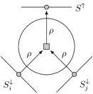
($\heartsuit$)

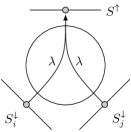
($\diamondsuit$)

Figure 3: Construction of the set $C_{B}$ for a branching bag $B$.

Before analysing the cardinality of $C_{\mathbb{B}}$ in Lemma 14 below, we need an axillary lemma.

Lemma 13

For a tree $T$ which is rooted in one of its leaves, let $b$ denote the number of branching nodes, $c$ denote the total number of children of branching nodes, and $l$ denote the number of leaves. Then, $c+b\leq 3l-1$ and $c\leq 2l-1$.

Proof

Assume that we construct $T$ by starting with only the root and then step by step adding leaves to it. Let $T_{i}$ be the subtree of $T$ with $i$ nodes during this construction. We define $b_{i}$, $c_{i}$, and $l_{i}$ accordingly. Now, assume by induction over $i$ that Lemma 13 is true for $T_{i}$. Let $v$ be the leaf we add to construct $T_{i+1}$ and let $u$ be its neighbour.

First, consider the case when $u$ is a leaf of $T_{i}$. Then, $u$ becomes a path node of $T_{i+1}$. Therefore, $b_{i+1}=b_{i}$, $c_{i+1}=c_{i}$, and $l_{i+1}=l_{i}$. Next, assume that $u$ is path node of $T_{i}$. Then, $u$ is a branch node of $T_{i+1}$. Thus, $b_{i+1}=b_{i}+1$, $c_{i+1}=c_{i}+2$, and $l_{i+1}=l_{i}+1$. Therefore, $c_{i+1}+b_{i+1}=c_{i}+b_{i}+3\leq 3(l_{i}+1)-1=3l_{i+1}-1$ and $c_{i+1}=c_{i}+2\leq 2(l_{i}+1)-1=2l_{i+1}-1$. It remains to check the case when $u$ is a branch node of $T_{i}$. Then, $b_{i+1}=b_{i}$, $c_{i+1}=c_{i}+1$, and $l_{i+1}=l_{i}+1$. Thus, $c_{i+1}+b_{i+1}=c_{i}+b_{i}+1\leq 3l_{i}-1+1\leq 3l_{i+1}-1$ and $c_{i+1}=c_{i}+1\leq 2l_{i}-1+1\leq 2l_{i+1}-1$. Therefore, in all three cases, Lemma 13 is true for $T_{i+1}$.  $\square$

Lemma 14

$|C_{\mathbb{B}}|\leq\phi\cdot\Lambda\big{(}T_{\phi}\big{)}$.

Proof

For some branching bag $B\in\mathbb{B}$, the set $C_{B}$ contains ($\heartsuit$)  a path of length at most $\rho$ for each $S_{i}\in\mathcal{S}^{\scriptscriptstyle\downarrow}(B)$ and a path of length at most $\rho$ to $S^{\raisebox{0.3014pt}{$\scriptscriptstyle\uparrow$}}(B)$, or ($\diamondsuit$)  a path of length at most $\lambda$ for each $S_{i}\in\mathcal{S}^{\scriptscriptstyle\downarrow}(B)$. Thus, ($\heartsuit$)  $|C_{B}|\leq\rho\cdot\big{|}\mathcal{S}^{\scriptscriptstyle\downarrow}(B)\big{|}+\rho$ or ($\diamondsuit$)  $|C_{B}|\leq\lambda\cdot\big{|}\mathcal{S}^{\scriptscriptstyle\downarrow}(B)\big{|}$. Recall that $\mathcal{S}^{\scriptscriptstyle\downarrow}(B)$ contains exactly one down-separator for each child of $B$ in $T_{\phi}$ and that $C_{\mathbb{B}}$ is the union of all sets $C_{B}$. Therefore, Lemma 13 implies the following.

$$|C_{\mathbb{B}}| \leq\sum_{B\in\mathbb{B}}|C_{B}|$$

($$\heartsuit \leq\rho\cdot\!\sum_{B\in\mathbb{B}}\big{|}\mathcal{S}^{\scriptscriptstyle\downarrow}(B)\big{|}+\rho\cdot|\mathbb{B}| \leq 3\rho\cdot\Lambda\big{(}T_{\phi}\big{)}-1$$)

($$\diamondsuit \leq\lambda\cdot\!\sum_{B\in\mathbb{B}}\big{|}\mathcal{S}^{\scriptscriptstyle\downarrow}(B)\big{|} \leq 2\lambda\cdot\Lambda\big{(}T_{\phi}\big{)}-1$$)

$$\leq\phi\cdot\Lambda\big{(}T_{\phi}\big{)}-1. \square$$  

Properties of $C_{\phi}$.

We now analyse the created set $C_{\phi}$ and show that $C_{\phi}$ is a connected $(r+\phi)$-dominating set for $G$.

Lemma 15

$C_{\phi}$ contains a vertex in each bag of $T_{\phi}$.

Proof

Clearly, by construction, $C_{\phi}$ contains a vertex in each path bag and in each branching bag. Now, consider a leaf $L$ of $T_{\phi}$. $L$ is adjacent to a path segment or branching bag $X\in\mathbb{P}\cap\mathbb{B}$. Whenever such an $X$ is processed, the algorithm ensures that all separators of $X$ contain a vertex of $C_{\phi}$. Since one of these separators is also the separator of $L$, it follows that each leaf $L$ and, thus, each bag of $T_{\phi}$ contains a vertex of $C_{\phi}$.  $\square$

Lemma 16

$|C_{\phi}|\leq|D_{r}|$.

Proof

Note that, for each vertex $u$ we add to $C_{\phi}$, we also add $u$ to a unique set $C_{X}$ for some $X\in\mathbb{P}\cap\mathbb{B}$. The exception is the vertex $v$ in $S^{\scriptscriptstyle\downarrow}(R)$ which is added to no such set $C_{X}$. It follows from our construction of the sets $C_{X}$ that there is only one such vertex $v$ and that $v=\nu\big{(}S^{\scriptscriptstyle\downarrow}(R)\big{)}$. Thus, $|C_{\phi}|=|C_{\mathbb{P}}|+|C_{\mathbb{B}}|+1$. Now, it follows from Lemma 12 and Lemma 14 that

$$|C_{\phi}|\leq|D_{r}|-\phi\cdot\Lambda\big{(}T_{\phi}\big{)}+\phi\cdot\Lambda\big{(}T_{\phi}\big{)}-1+1\leq|D_{r}|.$$

Lemma 17

$C_{\phi}$ is connected.

Proof

First, note that, by maximality, two path segments of $T_{\phi}$ cannot share a common separator. Also, note that, when processing a branching bag $B$, the algorithm first checks if, for any separator $S$ of $B$, $\nu(S)$ is already defined; if this is the case, it will not be overwritten. Therefore, for each separator $S$ in $T_{\phi}$, $\nu(S)$ is defined and never overwritten.

Next, consider a path segment or branching bag $X\in\mathbb{P}\cup\mathbb{B}$ and let $S$ and $S^{\prime}$ be two separators of $X$. Whenever such an $X$ is processed, our approach ensures that $C_{\phi}$ connects $\nu(S)$ with $\nu(S^{\prime})$. Additionally, observe that, when processing $X$, each vertex added to $C_{\phi}$ is connected via $C_{\phi}$ with $\nu(S)$ for some separator $S$ of $X$.

Thus, for any two separators $S$ and $S^{\prime}$ in $T_{\phi}$, $C_{\phi}$ connects $\nu(S)$ with $\nu(S^{\prime})$ and, additionally, each vertex $v\in C_{\phi}$ is connected via $C_{\phi}$ with $\nu(S)$ for some separator $S$ in $T_{\phi}$. Therefore, $C_{\phi}$ is connected.  $\square$

From Lemma 15, Lemma 16, Lemma 17, and from applying Lemma 11 it follows:

Corollary 6

$C_{\phi}$ is a connected $\big{(}r+(\phi+\lambda)\big{)}$-dominating set for $G$ with $|C_{\phi}|\leq|D_{r}|$.

Implementation.

Algorithm 6 below implements our approach described above. This also includes the case when $T_{\phi}$ contains at most two bags.

1

2($\heartsuit$) Set $\phi:=3\rho$.

3 ($\diamondsuit$) Set $\phi:=2\lambda$.

4Compute a minimum $(r+\phi)$-covering subtree $T_{\phi}$ of $\mathcal{T}$ using Algorithm 4.

5if $T_{\phi}$ contains only one bag $B$  then

6      Pick an arbitrary vertex $u\in B$, output $C_{\phi}:=\{u\}$, and stop.

7

8if $T_{\phi}$ contains exactly two bags $B$ and $B^{\prime}$  then

9      Pick an arbitrary vertex $u\in B\cap B^{\prime}$, output $C_{\phi}:=\{u\}$, and stop.

10

11Pick a leaf of $T_{\phi}$ and make it the root of $T_{\phi}$.

12Split $T_{\phi}$ into a set $\mathbb{L}$ of leaves, a set $\mathbb{P}$ of path segments, and a set $\mathbb{B}$ of branching bags.

13Create an empty set $C_{\phi}$.

14foreach $P\in\mathbb{P}$  do

15      Find a shortest path $Q_{P}$ from $S^{\raisebox{0.3014pt}{$\scriptscriptstyle\uparrow$}}(P)$ to $S^{\scriptscriptstyle\downarrow}(P)$ and add its vertices into $C_{\phi}$.

16      Let $x\in S^{\raisebox{0.3014pt}{$\scriptscriptstyle\uparrow$}}(P)$ be the start vertex and $y\in S^{\scriptscriptstyle\downarrow}(P)$ be the end vertex of $Q_{P}$. Set $\nu\big{(}S^{\raisebox{0.3014pt}{$\scriptscriptstyle\uparrow$}}(P)\big{)}:=x$ and $\nu\big{(}S^{\scriptscriptstyle\downarrow}(P)\big{)}:=y$.

17

18foreach $B\in\mathbb{B}$  do

19      If $\nu\big{(}S^{\raisebox{0.3014pt}{$\scriptscriptstyle\uparrow$}}(B)\big{)}$ is defined, let $u:=\nu\big{(}S^{\raisebox{0.3014pt}{$\scriptscriptstyle\uparrow$}}(B)\big{)}$. Otherwise, let $u$ be an arbitrary vertex in $S^{\raisebox{0.3014pt}{$\scriptscriptstyle\uparrow$}}(B)$ and set $\nu\big{(}S^{\raisebox{0.3014pt}{$\scriptscriptstyle\uparrow$}}(B)\big{)}:=u$.

20      ($\heartsuit$) Let $v:=c(B)$ be the center of $B$.

21       ($\diamondsuit$) Let $v:=u$.

22      Find a shortest path from $u$ to $v$ and add its vertices into $C_{\phi}$.

23      foreach $S_{i}\in\mathcal{S}^{\scriptscriptstyle\downarrow}(B)$  do

24            If $\nu(S_{i})$ is defined, let $w_{i}:=\nu(S_{i})$. Otherwise, let $w_{i}$ be an arbitrary vertex in $S_{i}$ and set $\nu(S_{i}):=w_{i}$.

25            Find a shortest path from $w_{i}$ to $v$ and add the vertices of this path into $C_{\phi}$.

26      

27

Output $C_{\phi}$.

Algorithm 6 Computes ($\heartsuit$)  a connected $(r+5\rho)$-dominating set or ($\diamondsuit$)  a connected $(r+3\lambda)$-dominating set for a given graph $G$ with a given tree-decomposition $\mathcal{T}$ with breadth $\rho$ and length $\lambda$.

Theorem 4.2

Algorithm 6 computes a connected $\big{(}r+(\phi+\lambda)\big{)}$-dominating set $C_{\phi}$ with $|C_{\phi}|\leq|D_{r}|$ in $\mathcal{O}(nm)$ time.

Proof

Since Algorithm 6 constructs a set $C_{\phi}$ as described above, its correctness follows from Corollary 6. It remains to show that the algorithm runs in $\mathcal{O}(nm)$ time.

Computing $T_{\phi}$ (line 6) can be done in $\mathcal{O}(nm)$ time (see Lemma 10). Picking a vertex $u$ in the case when $T_{\phi}$ contains at most two bags (line 6 to line 6) can be easily done in $\mathcal{O}(n)$ time. Recall that $T_{\phi}$ has at most $n$ bags. Thus, splitting $T_{\phi}$ in the sets $\mathbb{L}$, $\mathbb{P}$, and $\mathbb{B}$ can be done in $\mathcal{O}(n)$ time.

Determining all up-separators in $T_{\phi}$ can be done in $\mathcal{O}(M)$ time as follows. Process all bags of $T_{\phi}$ in an order such that a bag is processed before its descendants, e. g., use a preorder or BFS-order. Whenever a bag $B$ is processed, determine a set $S\subseteq B$ of flagged vertices, store $S$ as up-separator of $B$, and, afterwards, flag all vertices in $B$. Clearly, $S$ is empty for the root. Because a bag $B$ is processed before its descendants, all flagged vertices in $B$ also belong to its parent. Thus, by properties of tree-decompositions, these vertices are exactly the vertices in $S^{\raisebox{0.3014pt}{$\scriptscriptstyle\uparrow$}}(B)$. Clearly, processing a single bag $B$ takes at most $\mathcal{O}(|B|)$ time. Thus, processing all bags takes at most $\mathcal{O}(M)$ time. Note that it is not necessary to determine the down-separators of a (branching) bag. They can easily be accessed via the children of a bag.

Processing a single path segment (line 6 and line 6) can be easily done in $\mathcal{O}(m)$ time. Processing a branching bag $B$ (line 6 to line 6) can be implemented to run in $\mathcal{O}(m)$ time by, first, determining $\nu(S)$ for each separator $S$ of $B$ and, second, running a BFS starting at $v$ (defined in line 6) to connect $v$ with each vertex $\nu(S)$. Because $T_{\phi}$ has at most $n$ bags, it takes at most $\mathcal{O}(nm)$ time to process all path segments and branching bags of $T_{\phi}$.

Therefore, Algorithm 6 runs in $\mathcal{O}(nm)$ total time.  $\square$

5 Implications for the $p$-Center Problem

The (Connected) $p$-Center problem asks, given a graph $G$ and some integer $p$, for a (connected) vertex set $S$ with $|S|\leq p$ such that $S$ has minimum eccentricity, i. e., there is no (connected) set $S^{\prime}$ with $\operatorname{ecc}_{G}(S^{\prime})<\operatorname{ecc}_{G}(S)$. It is known (see, e. g., [3]) that the $p$-Center problem and $r$-Domination problem are closely related. Indeed, one can solve each of these problems by solving the other problem a logarithmic number of times. Lemma 18 below generalises this observation. Informally, it states that we are able to find a $+\phi$-approximation for the $p$-Center problem if we can find a good $(r+\phi)$-dominating set.

Lemma 18

For a given graph $G$, let $D_{r}$ be an optimal (connected) $r$-dominating set and $C_{p}$ be an optimal (connected) $p$-center. If, for some non-negative integer $\phi$, there is an algorithm to compute a (connected) $(r+\phi)$-dominating set $D$ with $|D|\leq|D_{r}|$ in $\mathcal{O}\big{(}T(G)\big{)}$ time, then there is an algorithm to compute a (connected) $p$-center $C$ with $\operatorname{ecc}_{G}(C)\leq\operatorname{ecc}_{G}(C_{p})+\phi$ in $\mathcal{O}\big{(}T(G)\log n\big{)}$ time.

Proof

Let $\mathcal{A}$ be an algorithm which computes a (connected) $(r+\phi)$ dominating set $D=\mathcal{A}(G,r)$ for $G$ with $|D|\leq|D_{r}|$ in $\mathcal{O}\big{(}T(G)\big{)}$ time. Then we can compute a (connected) $p$-center for $G$ as follows. Make a binary search over the integers $i\in[0,n]$. In each iteration, set $r_{i}(u)=i$ for each vertex $u$ of $G$ and compute the set $D_{i}=\mathcal{A}(G,r_{i})$. Then, increase $i$ if $|D_{i}|>p$ and decrease $i$ otherwise. Note that, by construction, $\operatorname{ecc}_{G}(D_{i})\leq i+\phi$. Let $D$ be the resulting set, i. e., out of all computed sets $D_{i}$, $D$ is the set with minimal $i$ for which $|D_{i}|\leq p$. It is easy to see that finding $D$ requires at most $\mathcal{O}\big{(}T(G)\log n\big{)}$ time.

Clearly, $C_{p}$ is a (connected) $r$-dominating set for $G$ when setting $r(u)=\operatorname{ecc}_{G}(C_{p})$ for each vertex $u$ of $G$. Thus, for each $i\geq\operatorname{ecc}_{G}(C_{p})$, $|D_{i}|\leq|C_{p}|\leq p$ and, hence, the binary search decreases $i$ for next iteration. Therefore, there is an $i\leq\operatorname{ecc}_{G}(C_{p})$ such that $D=D_{i}$. Hence, $|D|\leq|C_{p}|$ and $\operatorname{ecc}_{G}(D)\leq\operatorname{ecc}_{G}(C_{p})+\phi$.  $\square$

From Lemma 18, the results in Table 1 and Table 2 follow immediately.

Table 1: Implications of our results for the $p$-Center problem.

Approach	Approx.	Time
Layering Partition	$+\Delta$	$\mathcal{O}(m\log n)$
Tree-Decomposition	$+\rho$	$\mathcal{O}(nm\log n)$

Table 2: Implications of our results for the Connected $p$-Center problem.

Approach	Approx.	Time
Layering Partition	$+2\Delta$	$\mathcal{O}(m\,\alpha(n)\log\Delta\log n)$
Tree-Decomposition	$+\min(5\rho,3\lambda)$	$\mathcal{O}(nm\log n)$

In what follows, we show that, when using a layering partition, we can achieve the results from Table 1 and Table 2 without the logarithmic overhead.

Theorem 5.1

For a given graph $G$, a $+\Delta$-approximation for the $p$-Center problem can be computed in linear time.

Proof

First, create a layering partition $\mathcal{T}$ of $G$. Second, find an optimal $p$-center $\mathcal{S}$ for $\mathcal{T}$. Third, create a set $S$ by picking an arbitrary vertex of $G$ from each cluster in $\mathcal{S}$. All three steps can be performed in linear time, including the computation of $\mathcal{S}$ (see [15]).

Let $C$ be an optimal $p$-center for $G$. Note that, by Lemma 1, $C$ also induces a $p$-center for $\mathcal{T}$. Therefore, because $S$ induces an optimal $p$-center for $\mathcal{T}$, Lemma 1 implies that, for each vertex $u$ of $G$,

$$d_{G}(u,C)\leq d_{G}(u,S)\leq d_{\mathcal{T}}(u,\mathcal{S})+\Delta\leq d_{\mathcal{T}}(u,C)+\Delta\leq d_{G}(u,C)+\Delta.$$

Theorem 5.2

For a given graph $G$, a $+2\Delta$-approximation for the connected $p$-Center problem can be computed in $\mathcal{O}\big{(}m\,\alpha(n)\log\min(\Delta,p)\big{)}$ time.

Proof

Recall Algorithm 2 for computing a connected $(r+2\Delta)$-dominating set. We create Algorithm 2^∗ by slightly modifying Algorithm 2 as follows. In line 2, instead of computing an $r$-dominating subtree $T_{r}$ of $\mathcal{T}$, compute an optimal connected $p$-center $T_{p}$ of $\mathcal{T}$ (see [20]). Accordingly, in line 2, compute a $\delta$-dominating subtree of $T_{p}$, check in line 2 if $|S_{\delta}|\leq|T_{p}|$ (i. e., if $|S_{\delta}|\leq p$), and output in line 2 the set $S_{\delta}$ with the smallest $\delta$ for which $|S_{\delta}|\leq p$.

Let $S$ be the set computed by Algorithm 2^∗. As shown in the proof of Theorem 3.2, it follows from Lemma 6 and Corollary 2 that $S$ is connected, $|S|\leq p$, and $S=S_{\delta}$ for some $\delta\leq\Delta$.

Now, let $C$ be an optimal connected $p$-center for $G$. Clearly, by definition of $C$ and by Lemma 1, $\operatorname{ecc}_{G}(C)\leq\operatorname{ecc}_{G}(S_{\delta})\leq\operatorname{ecc}_{\mathcal{T}}(T_{\delta})+\Delta$. Because $T_{\delta}$ is a $\delta$-dominating subtree of $T_{p}$, $\operatorname{ecc}_{\mathcal{T}}(T_{\delta})\leq\operatorname{ecc}_{\mathcal{T}}(T_{p})+\delta$. Let $T_{C}$ be the subtree of $\mathcal{T}$ induced by $C$, i. e., the subtree of $\mathcal{T}$ induced by the clusters which contain vertices of $C$. Then, because $T_{p}$ is an optimal connected $p$-center for $\mathcal{T}$ and, clearly, $|T_{C}|\leq p$, $\operatorname{ecc}_{\mathcal{T}}(T_{p})\leq\operatorname{ecc}_{\mathcal{T}}(T_{C})$. Therefore, since $\delta\leq\Delta$, $\operatorname{ecc}_{G}(C)\leq\operatorname{ecc}_{G}(S_{\delta})\leq\operatorname{ecc}_{\mathcal{T}}(T_{C})+2\Delta$ and, by Lemma 1, $\operatorname{ecc}_{G}(C)\leq\operatorname{ecc}_{G}(S_{\delta})\leq\operatorname{ecc}_{G}(C)+2\Delta$.

As shown in the proof of Theorem 3.2, the one-sided binary search of Algorithm 2^∗ has at most $\mathcal{O}(\log\Delta)$ iterations. Because $|T_{p}|\leq p$, $T_{p}$ contains a cluster with eccentricity at most $\lceil p/2\rceil$ in $T_{p}$. Therefore, for any $\delta\geq\lceil p/2\rceil$, $|T_{\delta}|=|S_{\delta}|=1$ and, thus, the algorithm decreases $\delta$. Hence, the one-sided binary search of Algorithm 2^∗ has at most $\mathcal{O}(\log p)$ iterations. Therefore, the algorithm runs in at most $\mathcal{O}\big{(}m\,\alpha(n)\log\min(\Delta,p)\big{)}$ total time.  $\square$

References

- [1] Abboud, A., Williams, V.V., Wang, J., Approximation and fixed parameter subquadratic algorithms for radius and diameter in sparse graphs, Proceedings of the Twenty-Seventh Annual ACM-SIAM Symposium on Discrete Algorithms, 377–391, 2016.
- [2] Abu-Ata, M., Dragan, F.F., Metric tree-like structures in real-life networks: an empirical study Networks 67 (1), 49–68, 2016.
- [3] Brandstädt, A., Chepoi, V., and Dragan, F.F., The Algorithmic Use of Hypertree Structure and Maximum Neighbourhood Orderings. Discrete Applied Mathematics 82 (1–3), 43–77, 1998.
- [4] Brandstädt, A., Chepoi, V., and Dragan, F.F., Distance approximating trees for chordal and dually chordal graphs. Journal of Algorithms 30, 166–184, 1999.
- [5] Chepoi, V., Dragan, F.F., A note on distance approximating trees in graphs. European Journal of Combinatorics 21, 761–766, 2000.
- [6] Chepoi, V.D., Dragan, F.F., Estellon, B., Habib, M., Vaxes, Y., Diameters, centers, and approximating trees of -hyperbolic geodesic spaces and graphs, Proceedings of the 24th Annual ACM Symposium on Computational Geometry (SoCG 2008), 59–68, 2008.
- [7] Chepoi, V., Estellon, B., Packing and Covering -Hyperbolic Spaces by Balls, Lecture Notes in Computer Science 4627, 59–73, 2007.
- [8] Chlebík, M., Chlebíková, J., Approximation hardness of dominating set problems in bounded degree graphs, Information and Computation 206, 1264–1275, 2008.
- [9] Cormen, T.H., Leiserson, C.E., Rivest, R.L., Stein, C., Introduction to Algorithms (3. ed.), MIT Press, 2009.
- [10] Dourisboure, Y., Dragan, F.F., Gavoille, C., and Yan, C., Spanners for bounded tree-length graphs, Theoretical Computer Science 383 (1), 34–44, 2007.
- [11] Downey, R.G., Fellows, M.R., Parameterized Complexity, Springer, 1999.
- [12] Dragan, F.F., HT-graphs: centers, connected -domination and Steiner trees, Computer Science Journal of Moldova 1 (2), 64–83, 1993.
- [13] Edwards, K., Kennedy, K., Saniee, I., Fast Approximation Algorithms for -centers in Large -hyperbolic Graphs, WAW 2016, Lecture Notes in Computer Science 10088, 60–73, 2016.
- [14] Escoffier, B., Paschos, V.Th., Completeness in approximation classes beyond APX. Theoretical Computer Science 359 (1–3), 369–377, 2006.
- [15] Frederickson, G.N.: Parametric Search and Locating Supply Centers in Trees. WADS 1991, Lecture Notes in Computer Science 519, 299–319, 1991.
- [16] Gonzalez, T., Clustering to minimize the maximum intercluster distance, Theoretical Computer Science, 38, 293–306, 1985.
- [17] Guha, S., Khuller, S., Approximation algorithms for connected dominating sets, Algorithmica 20 (4), 374–387, 1998.
- [18] Niedermeier, R., Invitation to fixed-parameter algorithms, Oxford Lecture Series in Mathematics and Its Applications, Oxford University Press, 2006.
- [19] Raz, R., Safra, S., A sub-constant error-probability low-degree test, and sub-constant error-probability PCP characterization of NP, Proc. 29th Annual ACM Symposium on Theory of Computing, 475–484, 1997.
- [20] Yen, W.C.-K., Chen, C.-T.: The -center problem with connectivity constraint. Applied Mathematical Sciences 1 (27), 1311–1324, 2007.