A pedagogical description of diabatic and adiabatic molecular processes

Abstract

We provide a pedagogical approach to the problem of avoided crossings between electronic molecular curves and to diabatic and adiabatic transitions when the nuclei of a diatomic molecule move according to classical mechanics. For simplicity we restrict the analysis to only two electronic states.

1 Introduction

Several physical and chemical phenomena are commonly described in terms of the transition between adiabatic electronic curves that exhibit avoided crossings. Such models are useful, for example, in the study of the quenching of molecular species in electronically excited states by molecular gases[1], in photoinduced chemical reactions[2, 3], as well as in the Marcus theory for electrochemical reactions[4]. The transition between the adiabatic curves is typically described by means of the Landau-Zener formula[5, 6, 7]. This celebrated formula has been tested by means of simple models for pedagogical purposes[8]. In addition to these applications to physical chemistry and molecular physics we can also mention several models in classical mechanics developed as pedagogical illustrative examples[9, 10, 11, 12]. These classical models are useful to test the main assumptions of the approach by means of suitable devices that may be constructed in the laboratory[9, 10, 11].

The purpose of this paper is to provide an additional pedagogical analysis of the problem of avoided crossings and the adiabatic and diabatic transitions between electronic states. In section 2 we outline the Born-Oppenheimer approximation that is the source of the appearance of the potential-energy surfaces in the quantum-mechanical treatment of molecules. In section 3 we describe the avoided crossing between two potential-energy curves and show some illustrative results provided by a simple toy model. In section 4 we analyse earlier discussions on the avoided crossing between polar and nonpolar curves in alkali halides. In section 5 we briefly describe a semiclassical approach in which the nuclei move according to classical mechanics while the electronic states are treated by means of the time-dependent Schrödinger equation and illustrate the adiabatic and diabatic transitions between an initial and a final state. Finally, in section 6 we summarize the main results and draw conclusions.

2 The Born-Oppenheimer approximation

The non-relativistic, time-independent Schrödinger equation for a diatomic molecule with $N$ electrons is

$$H\psi = E\psi,$$

$$H = T_{n}+T_{e}+V_{ne}+V_{ee}+V_{nn},$$ (1)

where the kinetic energy of the nuclei $T_{n}$, the kinetic energy of the electrons $T_{e}$ and the electron-nuclei, electron-electron and nucleus-nucleus interactions $V_{ne}$, $V_{ee}$ and $V_{nn}$, respectively, are given by

$$T_{n} = -\frac{\hbar^{2}}{2}\left(\frac{\nabla_{A}^{2}}{M_{A}}+\frac{\nabla_{B}^{2}}{M_{B}}\right),$$

$$T_{e} = -\frac{\hbar^{2}}{2m}\sum_{j=1}^{N}\nabla_{j}^{2},$$

$$V_{ne} = -\frac{e^{2}}{4\pi\epsilon_{0}}\sum_{j=1}^{N}\left(\frac{Z_{A}}{r_{Aj}}+\frac{Z_{B}}{r_{Bj}}\right),$$

$$V_{ee} = \frac{e^{2}}{4\pi\epsilon_{0}}\sum_{i=1}^{N-1}\sum_{j=i+1}^{N}\frac{1}{r_{ij}},$$

$$V_{nn} = \frac{Z_{A}Z_{B}e^{2}}{4\pi\epsilon_{0}r_{AB}}.$$ (2)

In this expression $M_{A}$ and $M_{B}$ are the masses of the nuclei $A$ and $B$, respectively, $m$ is the electron mass, $Z_{A}$ and $Z_{B}$ are the atomic numbers, $r_{Aj}$ and $r_{Bj}$ are the distances of the electron $j$ to each nucleus, $r_{ij}$ is the distance between electrons $i$ and $j$, $r_{AB}=R$ is the distance between the nuclei and $\nabla^{2}$ denotes the Laplacian for every kind of particle.

The Born-Oppenheimer approximation consists in writing the eigenfunctions approximately as[13, 14]

$$\psi(\mathbf{r}_{j},R)\approx\psi^{e}(\mathbf{r}_{j};R)\psi^{n}(R),$$ (3)

where $\mathbf{r}_{j}$ stands for all the electron coordinates and the electronic and nuclear functions $\psi^{e}(\mathbf{r}_{j};R)$ and $\psi^{n}(R)$, respectively, are solutions to

$$H_{e}\psi^{e} = E^{e}(R)\psi^{e},$$

$$H_{e} = T_{e}+V_{ne}+V_{ee},$$ (4)

and

$$H_{n}\psi^{n} = E^{BO}\psi^{n},$$

$$H_{n} = T_{n}+U(R),$$

$$U(R) = E^{e}(R)+V_{nn}(R).$$ (5)

In this expression the Born-Oppenheimer energy $E^{BO}$ is the approximation to the actual molecular energy $E$.

In this analysis we have omitted the separation of the motion of the center of mass from the internal degrees of freedom that can be carried out in equation (5) or, more rigorously, in equation (1)[14]. In what follows we are interested in the clamped-nuclei equation (4) and such separation is not so relevant.

3 Avoided crossings

In the rest of the paper we restrict ourselves to the electronic equation (4) and for that reason we can omit the label $e$ on the electronic Hamiltonian, its eigenfunctions and eigenvalues, without causing (hopefully) any confusion. We suppose that we can obtain suitable approximations to a pair of electronic states by means of the Rayleigh-Ritz variational method with the simple trial function

$$\psi=c_{1}\varphi_{1}+c_{2}\varphi_{2},$$ (6)

where $\varphi_{1}$ and $\varphi_{2}$ are two suitable orthonormal functions and $c_{1}$ and $c_{2}$ are variational coefficients. These coefficients and the variational energies are solutions to the secular equations

$$\left(H_{11}-E\right)c_{1}+H_{12}c_{2} = 0,$$

$$H_{21}c_{1}+\left(H_{22}-E\right)c_{2} = 0,$$

$$H_{ij}=\left\langle\varphi_{i}\right|H\left|\varphi_{j}\right\rangle = H_{ji}^{*}.$$ (7)

We obtain nontrivial solutions if $E$ is a root of the secular determinant. The two roots of the characteristic polynomial

$$E_{1} = \frac{H_{11}+H_{22}}{2}-\frac{\Delta}{2},$$

$$E_{2} = \frac{H_{11}+H_{22}}{2}+\frac{\Delta}{2},$$

$$\Delta = \sqrt{\left(H_{11}-H_{22}\right)^{2}+4\left|H_{12}\right|^{2}}.$$ (8)

lead to the two approximate electronic states

$$\psi_{1} = c_{11}\varphi_{1}+c_{21}\varphi_{2},\;\frac{c_{21}}{c_{11}}=\frac{E_{1}-H_{11}}{H_{12}},$$

$$\psi_{2} = c_{12}\varphi_{1}+c_{22}\varphi_{2},\;\frac{c_{22}}{c_{12}}=\frac{E_{2}-H_{11}}{H_{12}},$$ (9)

where $\left|c_{1j}\right|^{2}+\left|c_{2j}\right|^{2}=1$.

The matrix elements $H_{ij}$ depend on the internuclear distance $R$ and we are interested in the case that $H_{11}(R)$ and $H_{22}(R)$ cross at $R=R_{c}$. For concreteness we assume that $H_{11}(R)<H_{22}(R)$ when $R<R_{c}$ and $H_{11}(R)>H_{22}(R)$ when $R>R_{c}$. If $H_{12}(R_{c})=0$ the adiabatic energies $E_{1}(R)$ and $E_{2}(R)$ cross at $R_{c}$ but if $H_{12}(R_{c})\neq 0$ we are in the presence of an avoided crossing. In the latter case the adiabatic energies approach each other as $R$ approaches $R_{c}$ and then move away as if repelling each other. At every $R$ the energy difference is $E_{2}(R)-E_{1}(R)=\Delta(R)$ and reaches its minimum at $R=R_{c}$, where $\Delta=2\left|H_{12}(R_{c})\right|$. At this point

$$\psi_{1} = \frac{1}{\sqrt{2}}\left(\varphi_{1}-\frac{\left|H_{12}\right|}{H_{12}}\varphi_{2}\right),$$

$$\psi_{2} = \frac{1}{\sqrt{2}}\left(\varphi_{1}+\frac{\left|H_{12}\right|}{H_{12}}\varphi_{2}\right).$$ (10)

Another common assumption is that $\left|E_{2}(R)-E_{1}(R)\right|\gg\left|H_{12}(R)\right|$ if $\left|R-R_{c}\right|$ is sufficiently large; therefore $\Delta\approx\left|H_{11}-H_{22}\right|$ under such condition. For $R\ll R_{c}$ $E_{1}\approx H_{11}$ and $E_{2}\approx H_{22}$; consequently $\psi_{1}\approx\varphi_{1}$ and $\psi_{2}\approx\varphi_{2}$. On the other hand, if $R\gg R_{c}$ $E_{1}\approx H_{22}$, $E_{2}\approx H_{11}$, $\psi_{1}\approx\varphi_{2}$ and $\psi_{2}\approx\varphi_{1}$. If $\varphi_{1}$ and $\varphi_{2}$ are associated to different physical behaviours of the system (for example, a polar or a nonpolar bond) we conclude that $\psi_{1}$ and $\psi_{2}$ change considerably when the system goes from $R\ll R_{c}$ to $R\gg R_{c}$ along an adiabatic curve.

Figure 1 shows results for a toy model given by $H_{11}(R)=1+R$, $H_{22}(R)=2-R$ and $H_{12}(R)=0.1$. The energies in the left panel and the square of the coefficient $\left|c_{1}(R)\right|^{2}$ in the right one clearly illustrate what we have just said. If we move from left to right along the lower curve in figure 1 left, we start in the state $\psi_{1}\approx\varphi_{1}$ and end in the state $\psi_{1}\approx\varphi_{2}$. On the other hand, if we follow the upper curve we start in the state $\psi_{2}\approx\varphi_{2}$ and end in the state $\psi_{2}\approx\varphi_{1}$. These are examples of adiabatic transitions in which we remain in the same adiabatic state $\psi_{j}$. If, on the other hand, we start in $\psi_{1}\approx\varphi_{1}$ to the left and go through the crossing towards the upper curve and end in $\psi_{2}\approx\varphi_{1}$ then we are in the presence of a diabatic transition. We will discuss these two processes with somewhat more detail in section 5.

4 Example

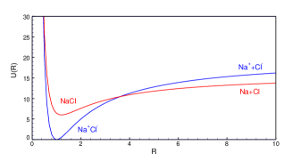
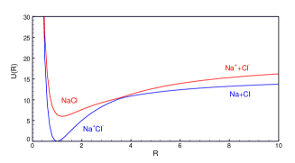
Figure 2: Diabatic (left) and adiabatic (right) curves for NaCl

Before proceeding with the general discussion of nonadiabatic transitions let us consider the well known example of the alkali halides. For example, Herzberg[15] mentions the avoided crossing between polar and nonpolar potential energy curves of NaCl which are schematically shown in figure 2. The left and right panels depict the diabatic and adiabatic curves $U(R)=E_{e}(R)+V_{nn}(R)$, respectively. Note that in the latter case the lowest electronic state changes from polar to nonpolar when going through the avoided crossing from left to right while the upper state behaves in the opposite way. The avoided crossing comes from the fact that both states are ${}^{1}\Sigma^{+}$ and cannot cross. Kauzmann[16] and Devaquet[3] carried out an analysis in terms of diabatic functions of the form

$$\chi_{ion} = \phi_{Cl}(1)\phi_{Cl}(2)\left(\alpha_{1}\beta_{2}-\beta_{1}\alpha_{2}\right),$$

$$\chi_{cov} = \left[\phi_{Cl}(1)\phi_{Na}(2)+\phi_{Na}(1)\phi_{Cl}(2)\right]\left(\alpha_{1}\beta_{2}-\beta_{1}\alpha_{2}\right),$$ (11)

where $\phi_{Na}$ and $\phi_{Cl}$ are $3S$ and $3p$ atomic orbitals, respectively.

According to Kauzmann: “The true wave function of the NaCl molecule is a hybrid of the above two

$$\psi=a\chi_{ion}+b\chi_{cov},$$ (12)

the coefficients $a$ and $b$ being functions of the interatomic distance, whose values, along with that of the corrected energy, may be found by means of the Rayleigh-Ritz method.” Devaquet[3] adds that “the gap $g$ between the adiabatic states (in the case where the overlaps between $\chi_{ion}$ and $\chi_{cov}$ is neglected) will be twice the matrix element $\left\langle\chi_{cov}\right|H\left|\chi_{ion}\right\rangle$ where $H$ denotes the total Hamiltonian of the molecule. Both one-electron and two-electron terms in $H$ will give contributions.” This analysis is appealing but unfortunately one cannot take it seriously because the authors failed to indicate why it is possible to describe the electronic structure of a 28-electron molecule by means of a pair of two-electron wavefunctions. One may reasonably ask about the meaning of the matrix element $\left\langle\chi_{cov}\right|H\left|\chi_{ion}\right\rangle$ of a 28-electron Hamiltonian between 2-electron functions. This kind of analysis should not be carried out (even on a qualitative basis) unless one defines a suitable model, which in this case means an effective two-electron Hamiltonian for an approximate description of the two valence electrons. Alternatively, one should indicate which 28-electron functions are schematically represented by the two-electron functions (12) that may probably be built by means of the valence bond method.

5 Time-evolution

In this section we discuss the time-evolution of an electronic molecular state due to the classical motion of the two nuclei. According to quantum mechanics the time-evolution of an state $\psi$ is given by the Schrödinger equation

$$i\hbar\frac{\partial}{\partial t}\psi=H\psi.$$ (13)

In order to derive general expressions it is convenient to consider an ansatz of the form

$$\psi=\sum_{j}c_{j}(t)e^{-ie_{j}(t)/\hbar}\varphi_{j},$$ (14)

where $\left\{\varphi_{j},\;j=1,2,\ldots\right\}$ is a complete set of suitable orthonormal functions independent of time

$$\frac{\partial\varphi_{j}}{dt}=0.$$ (15)

If $\psi$ is normalized at some initial time $t=t_{0}$ then it will be normalized at all times because $H$ is Hermitian

$$\sum_{j}\left|c_{j}(t)\right|^{2}=1.$$ (16)

The quantities $e_{j}(t)$ depend on time, have units of energy$\times$time and will be determined later. If we introduce the ansatz (14) into (13) we have

$$\sum_{j}\left(i\hbar\dot{c}_{j}+\dot{e}_{j}c_{j}\right)e^{-ie_{j}/\hbar}\varphi_{j}=\sum_{j}c_{j}e^{-ie_{j}/\hbar}H\varphi_{j},$$ (17)

where a point indicates time derivative. We now apply the ket $\left\langle\varphi_{n}\right|$ from the left

$$\left(i\hbar\dot{c}_{n}+\dot{e}_{n}c_{n}\right)e^{-ie_{n}(t)/\hbar}=\sum_{j}c_{j}e^{-ie_{j}/\hbar}H_{nj},\;H_{nj}=\left\langle\varphi_{n}\right|H\left|\varphi_{j}\right\rangle,\;n=1,2,\ldots,$$ (18)

and choose

$$\dot{e}_{n}=H_{nn},$$ (19)

in order to remove the diagonal terms

$$i\hbar\dot{c}_{n}=\sum_{j\neq n}c_{j}e^{iu_{nj}/\hbar}H_{nj},\;u_{nj}=\frac{e_{n}-e_{j}}{\hbar}.$$ (20)

It is worth noting that the derivatives

$$\dot{u}_{nj}=\frac{H_{nn}-H_{jj}}{\hbar}=\omega_{nj},$$ (21)

have units of angular frequency.

In order to apply these expressions to the two-level model discussed in section 3 we restrict them to the case that $n,j=1,2$; therefore, the system of equations (20) reduces to

$$i\hbar\dot{c}_{1} = c_{2}e^{iu_{12}/\hbar}H_{12},$$

$$i\hbar\dot{c}_{2} = c_{1}e^{iu_{21}/\hbar}H_{21},$$ (22)

where $u_{12}=-u_{21}$ and $H_{12}=H_{21}^{*}$. For simplicity we define

$$w=\frac{H_{12}e^{iu_{12}}}{\hbar},$$ (23)

that leads to somewhat simpler equations

$$\dot{c}_{1} = -iwc_{2},$$

$$\dot{c}_{2} = -iw^{*}c_{1}.$$ (24)

This problem is commonly analysed in terms of differential equations of second order[5, 6, 7]. To this end we differentiate the first equation in (24) with respect to time and then express $\dot{c}_{2}$ and $c_{2}$ in terms of $c_{1}$ and $\dot{c}_{1}$ using the same system of equations:

$$\ddot{c}_{1}=-i\dot{w}c_{2}-iw\dot{c}_{2}=\frac{\dot{w}}{w}\dot{c}_{1}-\left|w\right|^{2}c_{1}.$$ (25)

Analogously, we can derive a similar equation for $c_{2}$:

$$\ddot{c}_{2}=\frac{\dot{w}^{*}}{w^{*}}\dot{c}_{2}-\left|w\right|^{2}c_{2}.$$ (26)

If we assume that $\psi(t_{0})=\varphi_{1}$ (that is to say: $c_{1}(t_{0})=1$, $c_{2}(t_{0})=0$) then the initial conditions for the differential equation (25) are

$$c_{1}(t_{0})=1,\;\dot{c}_{1}(t_{0})=0.$$ (27)

The probability that the system remains in $\varphi_{1}$ at some $t>t_{0}$ is given by

$$P_{1}(t)=\left|\left\langle\varphi_{1}\right|\left.\psi(t)\right\rangle\right|^{2}=\left|c_{1}(t)\right|^{2}.$$ (28)

As argued in the preceding section $H_{11}(R)$ and $H_{22}(R)$ cross at $R=R_{c}$. We can expand all the relevant quantities in a Taylor series about this point:

$$\varphi_{k}(r_{j},R) = \varphi_{k}(r_{j},R_{c})+\varphi_{k}^{(1)}(r_{j},R_{c})\left(R-R_{c}\right)+\ldots.$$

$$H_{12}(R) = H_{12}(R_{c})+H_{12}^{(1)}(R_{c})\left(R-R_{c}\right)+\ldots.$$

$$H_{11}(R)-H_{22}(R) = \Delta H^{(1)}(R_{c})\left(R-R_{c}\right)+\ldots.$$ (29)

If we just keep the leading terms we can assume that $\varphi_{k}$ and $H_{12}$ are almost independent of $R$ in such a first-order approximation and that $H_{11}-H_{22}$ varies linearly with $R$. The coefficient

$$\Delta H^{(1)}(R_{c})=\left.\frac{\partial}{R}\left(H_{11}-H_{22}\right)\right|_{R=R_{c}},$$ (30)

will be relevant for subsequent discussion. Note that it is the difference between the slopes of $H_{11}(R)$ and $H_{22}(R)$ at the diabatic crossing $R=R_{c}$.

Let us assume that the nuclei move according to classical mechanics with a constant velocity $\dot{R}=v$ so that $R(t)=R_{0}+v\left(t-t_{0}\right)$. If $R\left(t_{c}\right)=R_{c}$ we have $R_{c}=R_{0}+v\left(t_{c}-t_{0}\right)$ and $R-R_{c}=v\left(t-t_{c}\right)$. Because of what we have just argued about equations (29) we conclude that the functions $\varphi_{k}$ are independent of time, which is consistent with equation (15), and that

$$\frac{dH_{12}}{dt}=0.$$ (31)

For this reason

$$\dot{w}=i\dot{u}_{12}w=i\frac{H_{11}-H_{22}}{\hbar}w=i\omega_{12}w,$$ (32)

and equation (25) becomes

$$\ddot{c}_{1}=i\omega_{12}\dot{c}_{1}-\left|w\right|^{2}c_{1},\;\left|w\right|=\frac{\left|H_{12}\right|}{\hbar}.$$ (33)

From all the assumptions outlined above we conclude that

$$\omega_{12}=\frac{H_{11}-H_{22}}{\hbar}=\frac{\alpha\left(t-t_{c}\right)}{\hbar},\;\alpha=\Delta H^{(1)}v.$$ (34)

Thus, the differential equation of second order becomes

$$\ddot{c}_{1}=i\frac{\alpha\left(t-t_{c}\right)}{\hbar}\dot{c}_{1}-\left|w\right|^{2}c_{1}.$$ (35)

All the calculations are much simpler if we work with dimensionless equations with the smallest number of model parameters. To this end we define the dimensionless time

$$s=\left|w\right|\left(t-t_{c}\right)=\left|\frac{H_{12}}{\hbar}\right|\left(t-t_{c}\right),$$ (36)

so that

$$c_{1}^{\prime\prime}=i\lambda sc_{1}^{\prime}-c_{1},\;\lambda=\frac{\alpha}{\hbar\left|w\right|^{2}}=\frac{\hbar\alpha}{\left|H_{12}\right|^{2}}=\frac{\hbar\Delta H^{(1)}v}{\left|H_{12}\right|^{2}},$$ (37)

where the prime stands for derivative with respect to $s$. Since $\dot{c}_{1}=\left|w\right|c_{1}^{\prime}$, the boundary conditions become

$$c_{1}(s_{0})=1,\;c_{1}^{\prime}(s_{0})=0.$$ (38)

The advantage of equation (37) is that it depends on only one parameter $\lambda$. Note that it increases with the difference between the slopes of $H_{11}(R)$ and $H_{22}(R)$ at $R=R_{c}$, with the relative velocity of the nuclei and decreases with the magnitude of the gap between the adiabatic curves at $R=R_{c}$. When $\lambda=0$ the system simply oscillates between the two states: $c_{1}(s)=\cos\left(s-s_{0}\right)$.

Figure 3 shows $\left|c_{1}\right|^{2}(s)$ for $s_{0}=-10$ and two values of $\lambda$. We appreciate that the probability that the system remains in the state $\varphi_{1}$ when $s\rightarrow\infty$ agrees with the limit given by the celebrated Landau-Zener formula[5, 6, 7]

$$P_{1}=\exp\left(-\frac{2\pi}{\lambda}\right),$$ (39)

written in terms of the only parameter in the dimensionless equation (37). On the other hand, the probability of the transition from the state $\varphi_{1}$ to the state $\varphi_{2}$ is given by $P_{2}=1-P_{1}$. Note that $\left|c_{2}\right|^{2}(s)=1-$ $\left|c_{1}\right|^{2}(s)$ is the probability of a diabatic transition from the lower to the upper curve in figure 1 left. On the other hand, $\left|c_{1}\right|^{2}(s)$ is the adiabatic transition in which the system remains in the lower curve in that same figure. Figure 3 shows that the probability of an adiabatic transition increases with $\lambda$. We obtained the numerical data for this figure by means of the fourth-order Runge-Kutta method built in Derive[17] (see page 266).

In closing this section we mention that the Landau-Zener approach exhibits several limitations already summarized by Geltman and Aragon[8] in a pedagogical paper (more rigorous analyses can be seen in the references therein).

6 Conclusions

We have seen that two adiabatic potential-energy curves cannot cross unless their interaction vanishes at the crossing point. Commonly, they exhibit an avoided crossing that looks as if they repel each other. If the nuclei are treated as classical particles they can remain on the same adiabatic curve or move from one to the other (adiabatic and diabatic transitions, respectively). The probability of each of these processes is determined by the relative velocity of the nuclei, the slopes of the diabatic energies at the crossing and the gap between the adiabatic curves at such point. The process is described by a differential equation of second order that leads to the celebrated Landau-Zener formula for the transition probability[5, 6, 7]. There is a trick in the development of such differential equation: the functions $\varphi_{j}$ and the interaction $H_{12}$ are assumed to be time-independent while $H_{11}-H_{22}$ is time-dependent. That this approximation is sound can be verified experimentally by means of classical devices[9, 10, 11].

It is worth noting that the potential-energy curves (or, more generally, the potential-energy surfaces) appear in a quantum-mechanical description of molecular systems because of the application of the Born-Oppenheimer approximation[13, 14]. In this sense, we may say that the potential-energy surfaces are artifacts of such an approximation. It may be interesting to investigate how to obtain results and conclusions similar to those in the preceding sections without that approximation. In other words, how to describe the phenomena outlined above by means of the time-dependent Schrödinger equation with the complete Hamiltonian shown in equation (1).

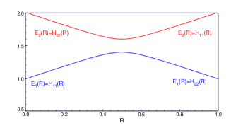
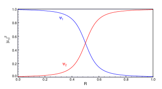
Figure 1: Approximate energies (left panel) of the two-level model shown in equations (6-9) and the contribution $\left|c_{1}\right|^{2}$ of $\varphi_{1}$ to the electronic states (right panel)

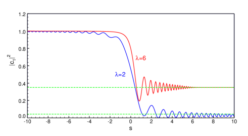
Figure 3: Probability that $\psi(s)=\varphi_{1}$ for two values of $\lambda$. The dashed (green) lines mark the Landau-Zener limits

References

- [1] E. Bauer, E. R. Fisher, and F. R. Gilmore, De-excitation of Electronically Excited Sodium by Nitrogen, J. Chem. Phys. 51 (1969) 4173-4181.
- [2] W. Th. A. M. Van der Lugt and L. J. Oosterhoff, Symmetry control and photoinduced reactions, J. Amer. Chem. Soc. 91 (1969) 6042-6049.
- [3] A. Devaquet, Avoided crossings in photochemistry, Pure Appl. Chem. 41 (1975) 455-473.
- [4] A. J. Bard and L. R. Faulkner, Electrochemical Methods. Fundamentals and Applications, Second (John Wiley & Sons, New York, 2001).
- [5] C. Zener, Non-Adiabatic Crossing of Energy Levels, Proc. R. Soc. London Ser. A137 (1932) 696-702.
- [6] J. R. Rubbmark, M. M. Kash, M. G. Littman, and D. Kleppner, Dynamical effects at avoided level crossings: A study of the Landay-Zerner effect using Rydberg atoms, Phys. Rev. A 23 (1981) 3107-3117.
- [7] C. Wittig, The Landau-Zener Formula, J. Phys. Chem. B 109 (2005) 8428-8430.
- [8] S. Geltman and N. D. Aaragon, Model study of the Landau-Zener approximation, Am. J. Phys. 73 (2005) 1050-1054.
- [9] H. J. Maris and X. Quan, Adiabatic and nonadiabatic processes in classical and quantum mechanics, Am. J. Phys. 56 (1988) 1114-1117.
- [10] W. Frank and P. von Brentano, Classical analogy to quantum mechanical level repulsion, Am. J. Phys. 62 (1994) 706-709.
- [11] B. W. Shore, M. V. Gromovyy, L. P. Yatsenko, and V. I. Romanenko, Simple mechanical analogs of rapid adiabatic passage in atomic physics, Am. J. Phys. 77 (2009) 1183-1194.
- [12] L. Novotny, Strong coupling, energy splitting, and level crossings: A classical perspective, Am. J. Phys. 78 (2010) 1199-1202.
- [13] M. Born and K. Huang, Dynamical Theory of Cristal Lattices, Oxford University Press, Glasgow, 1954).
- [14] F. M. Fernández and J. Echave, Nonadiabatic Calculation of Dipole Moments, in: J. Grunenberg (Ed.), Computational Spectroscopy. Methods, Experiments and Applications, Vol. Wiley-VCH, Weinheim, 2010.
- [15] G. Herzberg, Molecular Spectra and Molecular Structure. I. Spectra of Diatomic Molecules, Second (Van Nostrand Reinhold Company, New York, 1950).
- [16] W. Kauzmann, Quantum Chemistry, Academic Press, New York, 1957).
- [17] A. Rich, J. Rich, T. Shelby, and D. Stoutemyer, User Manual Derive, Seventh (Soft Warehouse, Honolulu, 1996).