Partial inertia induces additional phase transition in the explosive majority vote model

Abstract

Recently it has been aroused a great interest about explosive (i.e., discontinuous) transitions. They manifest in distinct systems, such as synchronization in coupled oscillators, percolation regime, absorbing phase transitions and more recently, in the majority-vote (MV) model with inertia. In the latter, the model rules are slightly modified by the inclusion of a term depending on the local spin (an inertial term). In such case, Chen et al. (Phys Rev. E 95, 042304 (2017)) have found that relevant inertia changes the nature of the phase transition in complex networks, from continuous to discontinuous. Here we give a further step by embedding inertia only in vertices with degree larger than a threshold value $\langle k\rangle k^{*}$, $\langle k\rangle$ being the mean system degree and $k^{*}$ the fraction restriction. Our results, from mean-field analysis and extensive numerical simulations, reveal that an explosive transition is presented in both homogeneous and heterogeneous structures for small and intermediate $k^{*}$’s. Otherwise, large restriction can sustain a discontinuous transition only in the heterogeneous case. This shares some similarity with recent results for the Kuramoto model (Phys Rev. E 91, 022818 (2015)). Surprisingly, intermediate restriction and large inertia are responsible for the emergence of an extra phase, in which the system is partially synchronized and the classification of phase transition depends on the inertia and the lattice topology. In this case, the system exhibits two phase transitions.

I Introduction

An explosive (discontinuous) transition occurs when an infinitesimal increase of the control parameter produces an abrupt change in macroscopic quantities. This kind of transition has attracted a lot of interest in the recent years, inspired by the discovery of a procedure (the “Achlioptas process”) that gives rise to an abrupt percolation transition in complex networks explosive1 ; explosive2 ; explosive3 ; explosive4 . While subsequent works have shown the Achlioptas process transition was, in fact, a continuous phase transition with unusual finite-size scaling continuous1 ; continuous2 ; continuous3 , many related models with alternative mechanisms showing genuinely discontinuous and anomalous transitions have now been discovered (see Ref. expreview and references therein).

One of these main examples appear in the context of coupled oscillators in which the Kuramoto Model (KM) kuramoto plays a central role. The original KM describes self-sustained coupled phase oscillators and exhibits a continuous phase transition at a critical coupling, beyond which a collective behavior is achieved. A few years ago, in a pioneering work, Gardeñes et al. prl2011 , discovered that a discontinuous phase transition to synchronization emerges as a consequence of the correlation between structure and local dynamics when a scale-free network is considered. Subsequent studies have confirmed the transition robustness under changing ingredients, such as lattice topology prl2011 , time delay peron , disorder skardal and inertia inertia . Analysis of the explosive transition in simpler structures, such as star graphs, for which exact treatment is possible tiago , also confirmed that the transition to collective behavior is discontinuous. Investigating the explosive synchronization in a generic complex network, Zhang et al. kurths have found that a positive correlation between the oscillators frequency and the degree of their corresponding vertices is the required condition for its appearance. More recently, Pinto et al. saa have verified that it suffices to fulfill above minimal requirement for the hubs (e.g. the vertices with higher degrees) for promoting an abrupt transition.

Besides dynamical systems, they manifest in markovian nonequilibrium reaction-diffusion processes. Two groups are important in this context: those presenting absorbing states and the up-down symmetric systems. In the former, distinct mechanisms, such as the inclusion of a quadratic term in the particle creation rates quadratic1 ; quadratic2 , the need of a minimal neighborhood for generating subsequent offsprings fiore14 , synergetic effects in multi species models scp1 ; scp2 or cooperative coinfection in multiple diseases epidemic models coinfect1 ; coinfect2 ; coinfect3 can be taken into account for shifting, from a continuous transition (belonging generically to the directed percolation (DP) universality class marr99 ; odor07 ; henkel ) to a discontinuous one.

The Majority Vote (MV) model is one of the simplest nonequilibrium up-down symmetric systems exhibiting an order-disorder phase transition mario92 . Extensive studies of this model in distinct lattice topologies (besides the usual regular ones) showed that the symmetry-breaking phase transition is not affected by the kind of the underlying networks chen1 , although the critical behavior results in set of critical exponents entirely different pereira . However, very recently, Chen et al. chen2 verified that the usual second-order phase transition in the majority vote (MV) becomes first-order when a term depending on the local density is included in the dynamics (an inertial effect).

Aimed at investigating how the network topology and inertial effects contribute to the emergence of the explosive transition in the MV model, in this work we include the inertia only in a given fraction of sites with degree $k$ larger than a threshold $\langle k\rangle k^{*}$. We observe that the MV transition remains explosive only for a low/intermediate fraction of restriction $k^{*}$ in homogeneous structures. On the other hand, in heterogeneous networks, it is sufficient to include inertia only in the hubs for promoting an abrupt behavior. Remarkably, a new feature induced by the partial (but large) inertia is the emergence of an extra phase, in which the system is partially synchronized, whose phase transition can be continuous or discontinuous, according to the inertia magnitude. In this region of the phase diagram, the system presents two phase transitions.

This paper is organized as follows: In Sec. II, we derive the mean field theory for the model. Next, numerical results are shown in Sec. III. Conclusions are drawn in Sec. IV.

II Model and mean field analysis

The MV model is defined in an arbitrary lattice topology, in which each node $i$ of degree $k_{i}$ is attached to a spin variable, $\sigma_{i}$, that can take the values $\sigma_{i}=\pm 1$. In the original case, with probability $1-f$ each node $i$ tends to align itself with its local neighborhood majority, and with complementary probability $f$, the majority rule is not followed. The quantity $f$ is a misalignment term whose increasing gives rise to an order-disorder (continuous) phase transition. Chen et al. chen2 added to the transition rate a term depending only on the local state $\sigma_{i}$, irrespectively the majority nearest neighbor spins. Mathematically, one has the following transition rate

$$w(\sigma_{i})=\frac{1}{2}\left\{1-(1-2f)\sigma_{i}S\left[(1-\theta)\sum_{j=1}^{k_{i}}\sigma_{j}/k_{i}+\theta\sigma_{i}\right]\right\},$$ (1)

where $\theta$ denotes the inertia strength and $S(X)$ is defined by $S(X)={\rm sign(X)}$ if $X\neq 0$ and $S(0)=0$. Note that for $\theta=0$ one recovers the original MV model, whose critical transition depends on the nodes distribution. In particular, for $\theta>0.5$, the dynamics is fully dominated by the inertia and no phase transition is observed chen2 .

The time evolution of the density $\rho_{k}$ of “up” spins ($\sigma_{i}=1$) of a node with degree $k$ given by

$$\frac{d}{dt}\rho_{k}=w_{-1\rightarrow 1}(1-\rho_{k})-\rho_{k}w_{1\rightarrow-1},$$ (2)

where $w_{-1\rightarrow 1}$ and $w_{1\rightarrow-1}$ denote the transition rates to states with opposite spin. In the steady state one has that

$$\rho_{k}=\frac{w_{-1\rightarrow 1}}{w_{-1\rightarrow 1}+w_{1\rightarrow-1}}.$$ (3)

The average magnetization of a node of degree $k$ is related to $\rho_{k}$ through the relation $m_{k}=2\rho_{k}-1$. Our first inspection of the inertia effect is carried out through a mean-field treatment. Here, we follow the ideas from Ref. romualdo ; chen2 , in which the transition rates in Eq. (2) are rewritten in terms of the majority and minority rules, given by

$$w_{-1\rightarrow 1}=(1-2f){\bar{P}_{-}}+f,$$ (4)

where ${\bar{P}_{-}}$ is the probability that the node $i$ of degree $k$, with spin $\sigma_{i}=-1$, changes its state according to the majority rule. In particular, ${\bar{P}_{-}}$ depends on the number $n_{k}^{-}$ of nearest neighbor $+$ spins in such a way that ${\bar{P}_{-}}=\sum_{n=\lceil n_{k}^{-}\rceil}^{k}(1-\frac{1}{2}\delta_{n,n_{k}^{-}})C_{n}^{k}p_{+1}^{n}p_{-1}^{k-n}$, where $p_{\pm 1}$ is the probability that one of its nearest-neighbors is in the spin state $\pm 1$. Since the quantity $n_{k}^{-}$ corresponds to the lower limit, it is evaluated from the condition $S(X)=0$, reading $n_{k}^{-}=\frac{k}{2(1-\theta)}$.

A similar expression is obtained by writing down the transition rate $w_{1\rightarrow-1}$ in terms of the minority rule (instead of the majority one)

$$w_{1\rightarrow-1}=(1-f)-(1-2f){\bar{P}_{+}},$$ (5)

where ${\bar{P}_{+}}$ also reads ${\bar{P}_{+}}=\sum_{n=\lceil n_{k}^{+}\rceil}^{k}(1-\frac{1}{2}\delta_{n,n_{k}^{+}})C_{n}^{k}p_{+1}^{n}p_{-1}^{k-n}$, but the bottom limit reads $n_{k}^{+}=\frac{k(1-2\theta)}{2(1-\theta)}$.

For large $k$, each term of the above binomial distributions ${\bar{P}_{\pm}}$ approach to gaussian ones with mean $m=kp_{+}$ and variance $\sigma^{2}=kp_{+}p_{-}$. So that

$${\bar{P}_{\pm}}\rightarrow\frac{1}{2}\left\{1\pm{\rm erf}\left[\sqrt{2k}\left(\frac{\theta}{2(1-\theta)}\pm y\right)\right]\right\},$$ (6)

where ${\rm erf(x)}$ denotes the error function and the nearest neighbor probability $p_{+}$ has been rewritten in terms of the quantity $y$ through the relation $p_{+}\equiv 1/2+y$.

For any node without degree correlation, the probability that a randomly nearest neighbor has degree $k$ is $kP(k)/\langle k\rangle$. Thus, $p_{+}$ and $\rho_{k}$ are related by $p_{+}=\sum_{k}kP(k)/\langle k\rangle\rho_{k}$ and finally we arrive at the following expression

$$y+1/2=\sum_{k}\frac{kP(k)}{\langle k\rangle}\frac{(1-2f){\bar{P}_{-}}+f}{1+(1-2f)({\bar{P}_{-}}-{\bar{P}_{+}})},$$ (7)

with ${\bar{P}_{\pm}}$ evaluated from Eq. (6). By splitting Eq. (7) in two parts, the first and second terms get restricted to the nodes in the absence of and with inertia respectively, in such a way that

$$y+1/2=\sum_{k=k_{0}}^{\langle k\rangle k^{*}-1}\frac{kP(k)}{2\langle k\rangle}[1+(1-2f){\rm erf}(\sqrt{2k}y)]+\sum_{k=\langle k\rangle k^{*}}^{\infty}\frac{kP(k)}{\langle k\rangle}\frac{1-(1-2f){\rm erf}\left[\sqrt{2k}\left(\frac{\theta}{2(1-\theta)}-y\right)\right]}{2-(1-2f)\{{\rm erf}\left[\sqrt{2k}\left(\frac{\theta}{2(1-\theta)}-y\right)\right]+{\rm erf}\left[\sqrt{2k}\left(\frac{\theta}{2(1-\theta)}+y\right)\right]\}},$$ (8)

where $k_{0}$ denotes the minimum degree. In particular, for $\theta=0$, Eq. (8) reduces to $y=\frac{1-2f}{2\langle k\rangle}\left\{\sum_{k}k[{\rm erf}(\sqrt{2k}y)]P(k)\right\}$, in consistency with results from Refs. chen1 ; chen2 .

Thus, the solution(s) of Eq. (8) give us the values of $y$, whose corresponding $\rho_{k}$’s are obtained from Eq. (3). The mean magnetization $|m|$ is achieved by summing over all values of $k$ with their correspondent weights $P(k)$, so that $|m|=2\left[\sum_{k}\rho_{k}P(k)\right]-1$.

Figs. 1 and 2 show (for $\langle k\rangle=20$), the behavior of $|m|$ versus $f$, for two distinct network topologies. The first is an Erdos-Renyi (ER) graph, a prototypical model of a homogeneous random network, with the degree distribution given by $P(k)=\langle k\rangle^{k}e^{-\langle k\rangle}/k!$. The second case is a representative description of heterogeneous networks, in which nodes are distributed according to the probability distribution $P(k)\sim k^{-\gamma}$. From now on, such case will be referred as power law (PL) graph. Here, we take $k_{0}=0$ for the ER and, for avoiding divergences when $k\rightarrow 0$ in the PL, we have imposed $k_{0}$ constrained to the mean degree $\langle k\rangle$ through the relation $k_{0}=\frac{\gamma-2}{\gamma-1}\langle k\rangle$.

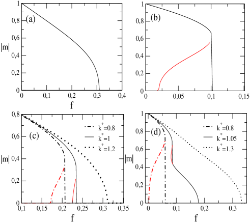
Figure 1: For the ER and $\langle k\rangle=20$, $|m|$ versus $f$ for distinct inertia rates. Panels $(a)$ and $(b)$ show the full inertia cases for $\theta=0.2$ and $0.4$, respectively. In panels $(c)$ and $(d)$, the restrictive case for $\theta=0.3$ and $\theta=0.45$ and distinct restrictions $k^{*}$’s. In all cases, red lines correspond the unstable branches.

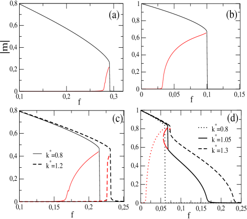
Figure 2: For the PL and $\langle k\rangle=20$, $|m|$ versus $f$ for distinct inertia rates. Panels $(a)$ and $(b)$ show the full inertia cases for $\theta=0.2$ and $0.4$, respectively. In panels $(c)$ and $(d)$, the restrictive case for $\theta=0.3$ and $\theta=0.45$ and distinct restrictions $k^{*}$’s. In all cases, red lines correspond the unstable branches.

As for ER and PL cases, top panels $(a)-(b)$ correspond to the full inertia cases whose phase transition is continuous for low $\theta$ and its increasing gives rise to a discontinuous one. Its emergence is signed by the appearance of an unstable branch (red lines), ending at to lower $f$’s when $\theta$ goes up. Despite the similarity between both cases, note the transition and the crossover (from continuous to discontinuous) points depend on $P(k)$. For example, for $\theta=0.2$ the transition is continuous for the ER and discontinuous for the PL. All these results are consistent with those obtained in Ref. chen2 .

Next, we examine the partial inertia case, in which the inertia appears only in a specific fraction of nodes (the ones with larger degrees). This analysis is inspired by the work by Pinto et al. saa for the KM, in which a positive correlation between frequency-degree taken only for the hubs is enough for promoting an explosive transition. For instance, we introduce the fraction parameter $k^{*}$, in such a way that $\theta\neq 0$ only if $k\geq\langle k\rangle k^{*}$ and $\theta=0$ otherwise. Extremely large $k^{*}$ implies that most of the nodes will be absent of inertia and thus the phase transition is expected to be similar to the $\theta=0$ case (continuous). In the opposite case, low $k^{*}$ makes the majority of sites to have inertia and one expects a scenario around the panels $(a)$ and $(b)$. Panels $(c)$ and $(d)$ in Figs. 1 and 2 show the results of the mean field theory (MFT) for the ER and PL [$\langle k\rangle=20$] and distinct sorts of $k^{*}$.

As expected, for low $k^{*}$’s MFT predicts similar behaviors than the full inertia cases (see, e.g., panels $(c)$ and $(d)$ for $k^{*}=0.8$). However, the increase of restriction leads to opposite scenarios. Whenever the discontinuous phase transition is suppressed for the ER when $k^{*}=1.2$, it is maintained for the PL. Despite a similar fraction of nodes with inertia (about $21\%$ and $17\%$ for the ER and PL, respectively), the presence of hubs in the PL sustains the discontinuous transition.

Surprising, an additional phase transition emerges for intermediate $k^{*}$’s and large $\theta$. This is clearly exemplified for $\theta=0.45$ and $k^{*}=1.05$ [panels $(d)$] in which the presence of a jump and an unstable envelope signals a discontinuous transition between two synchronized phases for low $f$ ($|m|\neq 0$ in both cases) followed by a smooth vanishing of $|m|$ for large $f$. In all cases, the transition between partially-ordered and disordered phase is continuous.

To examine such a new feature in more details, we plot in Fig. 3 the contribution of each part on the right side of Eq. (8) separately. That reveals the former transition comes from the subsystem with inertia (which becomes disordered), whereas the other gets ordered. By keeping the increase of $f$, the remaining subset (without inertia) also loses the ordering at $f_{c}$.

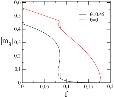
Figure 3: For the ER, $\langle k\rangle=20$ and $k^{*}=1.05$, the plot of the right side of Eq. (8) versus $f$ restricted to the inertial part ($\theta=0.45$ in the present case) and $\theta=0$. Dashed lines correspond to the unstable solutions.

In the next section, we continue the study of the effects of partial inertia through numerical simulations, in order to compare with our MFT predictions.

III Numerical results

We performed extensive numerical simulations of the MV model on random graphs with ER and PL topologies and system sizes $N$ ranging from $N=3600$ to $20000$. To construct an ER graph, we connect each pair of nodes with probability $\langle k\rangle/N$. When the size of the graph tends to infinity $N\to\infty$, its degree distribution is Poissonian, with mean $\langle k\rangle$. The PL graphs were generated using the uncorrelated configuration model (UCM) ucm , so the degrees are uncorrelated. As in the MFT, we use $\gamma=3$ and distinct sets of inertia values.

In order to classify the phase transition, we begin by analyzing the absolute value of the mean magnetization per site $|m|$ as a function of $f$, starting from a full ordered phase ($|m|=1$) and increasing $f$ towards the completely disordered phase ($|m|=0$). In sequence, we take the opposite case, wherein the system is in the disordered phase and the parameter $f$ is gradually decreased approaching to the ordered phase. Both increasing (“forward”) and decreasing (“backward”) curves are expected to coincide when the phase transition is critical, but they are different at the phase coexistence (a trademark of a discontinuous transition). The presence of hysteresis indicates the system bistability with respect to the ordered/disordered phase according to its initial condition. They are also signed by the presence of a bimodal probability distribution of the order-parameter $P(m)$. On the other hand, if the phase transition is continuous, $P(m)$ exhibits a single peak, whose position depends on $f$.

Another feature distinguishing them relies that the continuous case presents an algebraic divergence of its order parameter variance $\chi=N[\langle m^{2}\rangle-\langle m\rangle^{2}]$ at the critical point $f_{c}$ martins-fiore . (In simulations of finite systems, we observe a maximum that increases with the system size $N$). The transition point $f_{c}$ can also be identified through the reduced cumulant $U_{4}=1-\frac{\langle m^{4}\rangle}{3\langle m^{2}\rangle^{2}}$, since curves for distinct $N$’s cross at $f_{c}$. Off the critical point, $U_{4}\rightarrow 2/3$ and $0$ for the ordered and disordered phases, respectively when $N\rightarrow\infty$.

In order to compare with the MFT, Fig. 4 shows results for the ER and PL topologies and lower inertia values (exemplified here for $\theta=0.3$). In both cases, the presence of hysteresis for $k^{*}=0.8$ and $k^{*}=1$ reveal, in similarity with MFT, discontinuous transitions with hysteretic loop decreasing by elevating $k^{*}$. Also, the network structure leads to opposite features for $k^{*}=1.2$ with a continuous phase transition for the ER (panel $(b)$). The behavior is different for the PL (panel $(d)$), showing a small jump of $|m|$ at $f\sim 0.22$ for a partially ordered phase (see panel (d) in Fig. 4). This also contrasts with MFT results, in which a discontinuous order-disordered transition is predicted. Despite the evidence of a discontinuous transition for the PL, we believe that sufficient larger $N$’s are required for observing a hysteretic loop for such case.

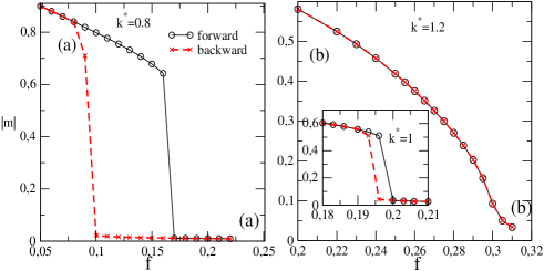
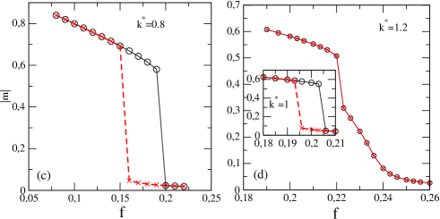
Figure 4: For ER [$(a)-(b)$] and PL [$(c)-(d)$] networks with $\theta=0.3$, the order parameter $|m|$ versus the control parameter $f$ for distinct $k^{*}$. Circles (stars) correspond the increase (decrease) of $f$ starting from an(a) ordered (disordered) phase. Except in panel $(d)$ ($N=40000$), results are for $N=20000$.

As in the MFT, numerical simulations also exhibit an additional phase transition for large $\theta$ and intermediate sets of $k^{*}$ (exemplified in Fig. 5 for $\theta=0.45$). Our results for low $f$ show a hysteretic loop signaling a phase coexistence between two synchronized phases (see panels $(a)$ and $(c)$ for $k^{*}=1.05$ and $1.1$, respectively), whereas by further increasing $f$, $|m|$ vanishes continuously. To achieve complementary information about the hysteretic loop, we evaluate the difference of magnetization restricted to the subsets of nodes with and without inertia ($m_{\theta}$ and $m_{0}$, respectively) given by $\phi=m_{\theta}-m_{0}$. For sufficient low $f$, $m_{\theta}\approx m_{0}\approx 1$, consistent with a full ordered phase. The jump of $\phi$ to a moderate value indicates that the nodes with inertia become unsynchronized, but the vertices absent of inertia remains ordered. Thus, in similarity with the MFT, we observe that the system, in fact, exhibits a partial synchronization. Although for $k^{*}=1.05$ the decrease of $f$ does not lead the system to the full synchronization (in similarity with the original order-disorder transition for large $\theta$), a closed hysteretic loop is observed for $k^{*}=1.1$. A bimodal distribution in the hysteretic region (inset) reinforces a discontinuous transition between partially-ordered and ordered phases. As expected for the ER, the additional transition is absent for $k^{*}=1.3$ (inset).

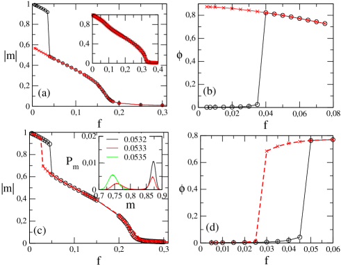
Figure 5: For the ER network of size $N=20000$ and $\theta=0.45$, panels $(a)$ and $(b)$ show $|m|$ and $\phi$ vs $f$ for $k^{*}=1.05$, respectively. Circles (stars) correspond the increase (decrease) of $f$ starting from an(a) ordered (disordered) phase. The same in panels $(c)$ and $(d)$, but for $k^{*}=1.1$. Insets: Top and bottom show $|m|$ vs $f$ for $k^{*}=1.3$ and the probability distribution $P(m)$ vs $m$ for distinct $f$’s and $N=3600$, respectively.

Now, we employ a finite size scaling analysis to characterize the order-disorder phase transition. In Fig. 6, we plot $\chi$ and $U_{4}$ for distinct network sizes $N$. We observe that they exhibit the typical behaviors expected for continuous phase transitions: the variance $\chi$ presents a maximum increasing with $N$ and their positions also systematically deviates on $N$. Analysis of $U_{4}$ (Fig. 6: panels $(b)$, $(d)$ and its inset) show crossings at $f_{c}=0.179(2)$, $f_{c}=0.236(3)$ and $f_{c}=0.330(5)$ with $U_{4}=0.27(2)$, close to the values found in Ref. pereira . Note that all critical points can be clearly distinguished from their previous hysteric loops.

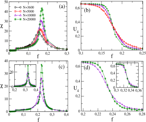
Figure 6: For the ER network and $\theta=0.45$, panels $(a)$ and $(b)$ show $\chi$ and $U_{4}$ vs $f$ for $k^{*}=1.05$. Panels $(c)$ and $(d)$, the same but for $k^{*}=1.1$. Insets: Results for $k^{*}=1.3$.

Similar trends are visualized in Fig. 7 where we show the results for PL networks with $k^{*}=1.05$ and $1.3$, respectively. However, in this case, the existence of hubs prolongs the partially synchronized discontinuous transition for a larger set of restrictions than the observed in ER networks.

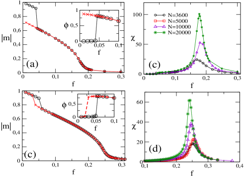
Figure 7: For the PL network and $\theta=0.45$, $|m|$ versus $f$ for $k^{*}=1.05$ [panel $(a)$] and $1.3$ [panel $(c)$]. Circles (stars) correspond the increase (decrease) of $f$ starting from an(a) ordered (disordered) phase. Insets show the order parameter $\phi$ vs $f$. Panels $(b)$ and $(d)$ shows the variance $\chi$ vs $f$ for distinct $N$’s.

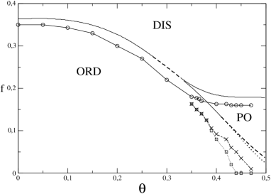
Figure 8: Phase diagram $f\times\theta$ for partial inertia $k^{*}=1.05$ and ER network with $\langle k\rangle=20$. ORD, DIS and PO denote the ordered, disordered and partially-ordered phases, respectively. Full lines correspond to the continuous transitions, whereas dashed (dotted) lines correspond to the increase (decrease) of $f$ starting from an(a) ordered (disordered) phase.

Figure 9: Phase diagram $f\times\theta$ for partial inertia $k^{*}=1.05$ and PL network with $\langle k\rangle=20$. In the left and right panels, numerical simulations for $N=20000$ and MFT, respectively. ORD, DIS and PO denote the ordered, disordered and partially-ordered phases, respectively. Full lines correspond to the continuous transitions, whereas dashed (dotted) lines correspond to the increase (decrease) of $f$ starting from an(a) ordered (disordered) phase.

In Fig. 8 we plot the phase diagram for the ER and $k^{*}=1.05$. As expected, both MFT and numerical simulations predict continuous transition between ordered (ORD) and disordered (DIS) phases for small $\theta$. MFT predicts the appearance of the partially ordered (PO) for $\theta\geq\theta_{c}=0.330(1)$, whose transition is continuous in the interval $\theta_{c}\leq\theta\leq 0.41$ and discontinuous for $\theta>0.41$. Numerical simulations exhibit an additional peak of $\chi$ (absent of hysteresis), consistent to the emergence of the PO for $0.36\leq\theta\leq 0.39$ and a clear hysteretic loop for $\theta>0.39$. Despite the excellent qualitative agreement between approaches, it is worth mentioning the difficulty of locating (and classifying) the PO phase transition for $\theta_{c}\leq\theta\leq 0.36$ under numerical simulations. Another point to mention concerns that the PO-DIS transition is always continuous and practically independent on the inertia for large $\theta$. A qualitative similar phase diagram is shown in Fig. 9 for the PL case. However, the ordered-PO transition line is always discontinuous, in qualitative agreement with MFT predictions.

IV Conclusions

Recently, Chen et al. chen2 have found that inertia is responsible for the appearance of an abrupt transition in the majority vote model in complex networks. In the present work, we advance by scrutinizing the inertia acting only in the most connected nodes. We show, through mean field analysis and numerical simulations for homogeneous and heterogeneous networks, that $partial$ inertia can change the system behavior depending on the inertia strength.

Our results also reveal that although relevant inertia rates are required for preserving the discontinuous transitions for homogeneous networks, this is not the case of heterogeneous structures, in which a rather small fraction a ($17\%$) already promotes an abrupt behavior. In other words, by including only such above fraction in the sites with larger degrees, the phase transition is discontinuous. This shares some similarities with the KM model, in which a positive frequency-degree correlation included only in the hubs is sufficient for sustaining an explosive synchronization saa .

A second remarkable effect of partial inertia concerns in the appearance of an additional phase characterized by a partial ordering of the system. The nature of the phase transition from the disordered phase to this partially ordered phase depends on the inertia strength. Therefore, there is a region in the phase diagram in which we observe two phase transitions: a continuous transition from the disordered to the partially ordered phase, and a discontinuous transition from the latter to the full ordered phase.

As pointed in chen2 , behavioral inertia is an essential characteristic of human being and animal groups. Therefore, inertia can be a significant ingredient in transitions that arise in social systems social , such as the emergence of a common culture social2 or the appearance of consensus sood and decision-making systems couzin . Our results suggest that inertia only in a small fraction of the population can produce dramatic effects if it is concentrated in the most connected individuals.

References

- (1) D. Achlioptas, R. M. D. Souza and J. Spencer, Science 323, 1453 (2009).
- (2) E. J. Friedman and A. S. Landsberg, Phys. Rev. Lett. 103, 255701 (2009).
- (3) F. Radicchi and S. Fortunato, Phys. Rev. Lett. 103, 168701 (2009).
- (4) Y. S. Cho, J. S. Kim, J. Park, B. Kahng, and D. Kim, Phys. Rev. Lett. 103, 135702 (2009).
- (5) R. A. da Costa, S. N. Dorogovtsev, A. V. Goltsev, and J. F. F. Mendes, Phys. Rev. Lett. 105, 255701 (2010).
- (6) P. Grassberger, C. Christensen, G. Bizhani, S.-W. Son, and M. Paczuski, Phys. Rev. Lett. 106, 225701 (2011).
- (7) O. Riordan and L. Warnke, Science 333, 322 (2011).
- (8) R. M. D.Souza and J. Nagler, Nat. Phys. 11, 531 (2015).
- (9) Y. Kuramoto, in Proceedings of the International Symposium on Mathematical Problems in Theoretical Physics, University of Kyoto, Japan, Lect. Notes in Physics 30, 420 (1975), edited by H. Araki.
- (10) J. Gómez-Gardeñes, S. Gómez, A. Arenas and Y. Moreno, Phys. Rev. Lett. 106, 128701 (2011).
- (11) T. K. D. Peron and F. A. Rodrigues, Phys. Rev. E 86, 016102 (2012).
- (12) Per S. Skardal and A. Arenas, Phys. Rev. E 89, 062811 (2014).
- (13) P. Ji, T. K. D. M. Peron, P. J. Menck, F. A. Rodrigues and J. Kurths, Phys. Rev. Lett. 110, 218701 (2013).
- (14) V. Vlasov, Y. Zou and T. Pereira, Phys. Rev. E 92, 012904 (2015).
- (15) X. Zhang, X. Hu, J. Kurths and Z. Liu, Phys. Rev. E 88, 010802(R) (2013).
- (16) R. S. Pinto and A. Saa, Phys, Rev. E 91, 022818 (2015).
- (17) Da-Jiang Liu, Xiaofang Guo, and James W. Evans, Phys. Rev. Lett. 98, 050601 (2007)
- (18) C. Varghese and R. Durrett, Phys. Rev. E 87, 062819 (2013).
- (19) C.E Fiore, Phys. Rev. E 89, 022104 (2014).
- (20) M. M. de Oliveira, R. V. Dos Santos, and R. Dickman, Phys. Rev. E 86, 011121 (2012).
- (21) M. M. de Oliveira and R. Dickman Phys. Rev. E 90, 032120 (2014).
- (22) L. Chen, F. Ghanbarnejad, W. Cai, and P. Grassberger, EPL 104, 50001 (2013).
- (23) W. Cai, L. Chen, F. Ghanbarnejad, and P. Grassberger, Nat. Phys. 4, 2412 (2015).
- (24) L. Hebert-Dufresnea and B. M. Althousea, Proc. Natl. Acad. Sci. USA 112, 10551 (2015).
- (25) J. Marro and R. Dickman, Nonequilibrium Phase Transitions in Lattice Models (Cambridge University Press, Cambridge, 1999).
- (26) G. Ódor, Universality In Nonequilibrium Lattice Systems: Theoretical Foundations (World Scientific,Singapore, 2007)
- (27) M. Henkel, H. Hinrichsen and S. Lubeck, Non-Equilibrium Phase Transitions Volume I: Absorbing Phase Transitions (Springer-Verlag, The Netherlands, 2008).
- (28) M. J. de Oliveira, J. Stat. Phys. 66, 273 (1992).
- (29) H. Chen, C. Shen, G. He, H. Zhang and Z. Hou, Phys, Rev. E 91, 022816 (2015).
- (30) L. F. C. Pereira and F. G. B. Moreira, Phys. Rev. E 71, 016123 (2005).
- (31) H. Chen, C. Shen, H. Zhang, G. Li, Z. Hou and J. Kurths, Phys Rev. E 95, 042304 (2017).
- (32) C. Castellano and R. Pastor-Satorras, J. Stat. Mech. p. P05001 (2006).
- (33) M. Catanzaro, M. Boguna and R. Pastor-Satorras, Phys. Rev. E 71, 027103 (2005).
- (34) M. M. de Oliveira, M. G. E. da Luz and C. E. Fiore, Phys. Rev. E 92, 062126 (2015).
- (35) C. Castellano, S. Fortunato, and V. Loreto, Rev. Mod. Phys. 81, 591 (2009).
- (36) C. Castellano, M. Marsili, and A. Vespignani, Phys. Rev. Lett. 85, 3536 (2000).
- (37) V. Sood and S. Redner, Phys. Rev. Lett. 94, 178701 (2005).
- (38) A. T. Hartnett, E. Schertzer, S. A. Levin, and I. D. Couzin, Phys. Rev. Lett. 116, 038701 (2016).