Learning Spatial-Aware Regressions for Visual Tracking

Abstract

In this paper, we analyze the spatial information of deep features, and propose two complementary regressions for robust visual tracking. First, we propose a kernelized ridge regression model wherein the kernel value is defined as the weighted sum of similarity scores of all pairs of patches between two samples. We show that this model can be formulated as a neural network and thus can be efficiently solved. Second, we propose a fully convolutional neural network with spatially regularized kernels, through which the filter kernel corresponding to each output channel is forced to focus on a specific region of the target. Distance transform pooling is further exploited to determine the effectiveness of each output channel of the convolution layer. The outputs from the kernelized ridge regression model and the fully convolutional neural network are combined to obtain the ultimate response. Experimental results on two benchmark datasets validate the effectiveness of the proposed method.

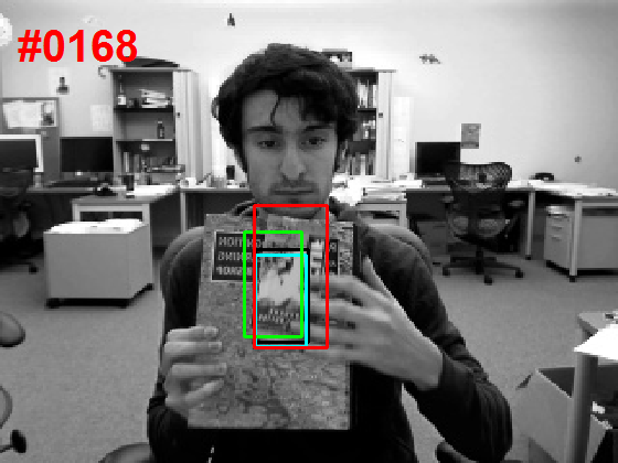
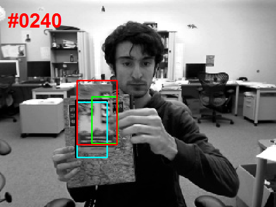
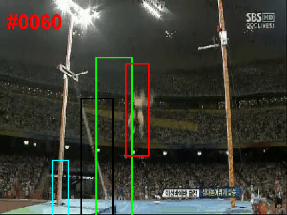
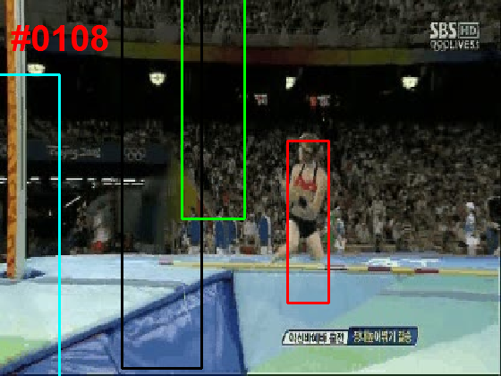
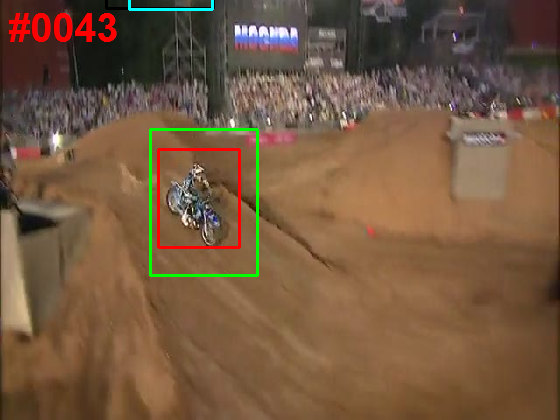
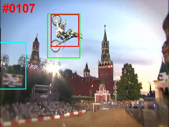
Figure 1: Example tracking results of different methods on the OTB dataset. Our tracker (LSART) has comparable results compared with the state-of-the-art algorithms.

1 Introduction

Visual tracking, which aims to continuously estimate the positions and scales of a pre-specified target, has been a hot topic for the last decades. It is widely used in numerous vision tasks, such as video surveillance, augmented reality and so on. Current algorithms have achieved very impressive results, however, many problems remain to be solved.

With the emergence of large-scale datasets, deep neural networks have shown their great capacity in object classification, image identification, to name a few. It has been verified in many prior papers [31, 25, 22] that trackers based on convolutional neural networks (CNNs) can significantly improve the tracking performance. Usually, these methods pretrain their networks on a large scale dataset, and finetune the networks with the ground-truth data in the first frame of a sequence. In addition to the CNN-based trackers, methods based on the kernelized correlation filter (KCF) are also very popular in recent years for the efficiency and capacity to utilize large numbers of negative samples. As is described in [17], the KCF method is essentially the kernelized ridge regression (KRR) with cyclically shifted samples. Methods based on the KCF usually take a region of interest as the input, which makes it very difficult to exploit the structural information of the target. In addition, the cyclically constructed samples also introduce the unwanted boundary effects. Compared to the KCF method, the dominating reason why the conventional KRR is not widely applied is that it has to compute a kernel matrix for large numbers of samples, which results in heavy computational load.

Both the CNN-and KRR-based trackers have limitations and they have complementarities. The CNN-based trackers usually contain a large number of parameters which are difficult to be finetuned in the tracking problem. As a result, the trained filter kernels in the convolution layer are usually highly correlated and tend to overfit the training data. On the contrary, the KRR-based trackers have limited model parameters (equal to the number of training samples), and cannot learn discriminative enough models when training samples are correlated. In addition, the existing KRR-based methods assume that each part of the target is equally important, and ignore the relationship among different parts.

In this paper, we exploit both the KRR and CNN models, and learn the complementary spatial-aware regressions for visual tracking (LSART). First, we propose a kernelized ridge regression with cross-patch similarities. We assign each similarity score a weight, and simultaneously learn this weight and ridge regression model parameters. We show that the proposed ridge regression model can be reformulated as a neural network, which is more efficiently optimized than the original form. Second, we introduce the spatially regularized kernels into the fully convolutional neural network. By imposing spatial constraints on the filter kernels, we enforce each output channel of the convolution layer to have a response for a specific localized region. We exploit the distance transform pooling layer to determine the effectiveness of the outputs from the convolution layer, and develop a two-stage training strategy to update the CNN model effectively. Finally, the heat maps obtained by the KRR and CNN models are combined to generate a final heat map for target location. Experiments on the popular datasets demonstrate that our tracker performs significantly better than other state-of-the-art methods (see Figure 1 for visualized tracking results).

The main contributions of this paper can be summarized as follows:

1. We develop a spatial-aware KRR model by introducing a cross-patch similarity kernel. This model can model both regression coefficients and patch reliability, which enables our model to be robust to the unreliable patches. The regression coefficient and similarity weight vectors are simultaneously optimized via an end-to-end neural network, which is new in visual tracking and facilitates seamlessly integrating our model with deep feature extraction networks.

2. We propose the spatially regularized filter kernels for CNN, which enforces each filter kernel to focus on a localized region. We also design a two-stream training network to effectively learn network parameters, which avoids overfitting and considers rotation information.

3. We propose the complementary KRR and CNN models based on their inherent limitations. The spatial-aware KRR model focuses on the holistic object and the spatial-aware CNN model focuses on small and localized regions, thereby complementing each other for better performance.

4. Our method achieves very promising tracking performance, especially on the recent VOT-2017 public dataset.

2 Related Work

Algorithms of visual tracking mainly focus on designing robust appearance models, which are roughly categorized as generative and discriminative models. With the progress of deep neural networks and correlation filters, discriminative appearance models are preferred in the recent works.

Trackers based on correlation filter have attracted more and more attention for the advantages in efficiency and robustness. In essential, correlation filter can be viewed as a kernelized ridge regression (KRR) model that can be speeded up in the frequency domain. Bolme et al. [3] exploit the correlation filter with minimum output sum of squared error for visual tracking. As fast Fourier transform is used, the tracker achieves very fast tracking performance. In [16], Henriques et al. first incorporate kernel functions into the correlation filter, which is named as CSK. The CSK tracker can also be solved via fast Fourier transform, thus is efficient. Based on [16], the tracking method [17] further improves the CSK tracker by using the histogram of gradient features. Ma et al. [23] exploit complementary nature of features extracted from three layers of CNN, and use a coarse-to-fine scheme for target searching. Based on [23], an online adaptive Hedge method [26] is designed, which takes both the short-term and long-term regrets into consideration. In this method, they use the CF-based tracker defined on a single CNN layer as an expert and learn the adaptive weights for different experts. Danelljan et al. propose several CF-based trackers with good performance. The SRDCF method [8] tries to suppress the boundary effects of the correlation filter by multiplying the filter coefficients with spatial regularization weights produced by a Gaussian distribution. This tracker achieves very good performance even with hand-crafted features. Based on [8], they propose an adaptive decontamination method [9] for the correlation filter, which adaptively learns the reliability of each training sample and eliminates the influence of contaminated ones. Furthermore, the learning process for correlation filter is conducted in the continuous spatial domain of various feature maps [10], which incorporates the sub-pixel information. These methods usually exploit the linear or Gaussian kernel to depict the similarity between the target region and a given candidate region. They inevitably ignore the intrinsic structure information within the target region, which makes the trackers be less effective in dealing with occlusion and deformation challenges. In this work, we introduce a novel kernel to model the cross-patch similarities, develop the corresponding KRR optimization model, and provide a network structure to solve it efficiently.

Compared with trackers based on correlation filters, CNN-based trackers also achieve good performance in recent years. In [21], a shallow network with two convolution layers is proposed, which learns the feature representation and classifier simultaneously. In [31], Wang et al. transfer the model pre-trained on image classification dataset to visual tracking and exploit the fully convolutional neural network for target location. Wang et al. [32] propose a sequentially training fashion for neural network to avoid the overfitting problem. Tao et al. [29] off-line train a Siamese deep neural network on large amounts of extra video sequences, and directly apply this model to conduct the optimal match during the tracking process. In [25], a multi-domain CNN-based tracker is proposed, in which the shared layers are used to obtain generic target representation and the domain specific layers are adopted for classification. These CNN-based trackers usually exploit the global information regarding the target object and therefore ignore its spatial layouts. To address this issue, we propose a convolution layer with spatially regularized filter kernels to focus on local regions of the target. Besides, we effectively combine the proposed KRR and CNN models to develop a robust tracker.

3 Spatial-Aware KRR

3.1 KRR with Cross-Patch Similarity (KRRCPS)

Given $N$ training samples $\{({{\bf x}_{i}},{y_{i}})\}_{i=1}^{N}$ in frame $t$, the conventional ridge regression can be formulated as

$${\bf w}_{t}=\arg\min_{{\bf w}_{t}}\sum\limits_{i}{{{({y_{i}}-{{\bf{w}}_{t}^{\top}}{{\bf{x}}_{i}})}^{2}}+\lambda{{\left\|{\bf{w}}_{t}\right\|}^{2}}},$$ (1)

where ${{\bf x}_{i}}\in\mathbb{R}^{d\times 1}$ denotes the feature vector for sample $i$, and $y_{i}$ is its sample label. In Eq. 1, ${\bf w}_{t}\in\mathbb{R}^{d\times 1}$ denotes the linear weight vector, and $\lambda$ is a regularization constant. According to the representer theorem [28], the model parameter ${\bf w}_{t}$ can be determined as the weighted sum of the training samples (i.e., ${\bf{w}}_{t}=\sum\limits_{i=1}^{N}{{\alpha_{i}}^{t}{{\bf{x}}_{i}}}$). Thus, the optimization problem (1) can be rewritten as

$${\bm{\alpha}}_{t}^{*}=\arg\min_{{\bm{\alpha}}_{t}}\sum\limits_{i=1}^{N}{{{({y_{i}}-\sum\limits_{j=1}^{N}{{\alpha_{j}^{t}}{k_{ij}}})^{2}}}+\lambda}\sum\limits_{i,j=1}^{N}{\alpha_{i}^{t}\alpha_{j}^{t}{k_{i,j}}},$$ (2)

where $\alpha_{i}^{t}$ is the weight for sample $i$, ${\bm{\alpha}}_{t}=\left[\alpha_{1}^{t},...,\alpha_{N}^{t}\right]^{\top}\in\mathbb{R}^{N\times 1}$, and $k_{i,j}$ is the kernel value computed between features ${\bf x}_{i}$ and ${\bf x}_{j}$. The existing kernel definitions (e.g., linear kernel and Gaussian kernel) do not fully consider the spatial layouts of the target, which limits the tracking performance.

In this work, we introduce a kernel function which considers the similarity of all pairs of patches between two samples. Especially, we divide each sample $i$ into $M$ patches, and obtain features for each patch $m$ as ${\bf x}_{i}^{m}$, then the kernel value between sample $i$ and $j$ is computed as

$${k_{ij}}=\sum\limits_{m,n=1}^{M}{{\beta_{m,n}^{t}}{{{\bf{x}}_{i}^{m}}^{\top}}}{\bf{x}}_{j}^{n},$$ (3)

where $\beta_{m,n}^{t}$ denotes the weight for the similarity score between $m$-and $n$-th patches. This kernel function has at least two advantages: (a) for each similarity score, the kernel function assigns a learnable weight to make the model adaptively focus on the similarity scores of reliable regions; (b) more similarity pairs between patches are considered, thereby enhancing the discriminant ability of the model.

By substituting Eq.3 into Eq.2 and introducing a regularization term, we obtain the optimization problem (4).

$${\bm{\alpha}}_{t}^{*},{\bm{\beta}}_{t}^{*}=\arg\mathop{\min}\limits_{{{\bm{\alpha}}_{t}},{{\bm{\beta}}_{t}}}J\left({{{\bm{\alpha}}_{t}},{{\bm{\beta}}_{t}}}\right),$$ (4)

where we define $J\left({{\bm{\alpha}},{\bm{\beta}}}\right)$ as

$$\begin{gathered}J\left({{\bm{\alpha}},{\bm{\beta}}}\right)\hfill\\ =\sum\limits_{i=1}^{N}{({y_{i}}-\sum\limits_{j=1}^{N}{\alpha_{j}^{t}\sum\limits_{m,n=1}^{M}{\beta_{m,n}^{t}{\mathbf{x}}{{{}_{j}^{m}}^{\top}}{\mathbf{x}}_{i}^{n}}{)^{2}}}}\hfill\\ \;\;\;\;+{\lambda_{1}}\sum\limits_{i,j=1}^{N}{\alpha_{i}^{t}}{k_{i,j}}\alpha_{j}^{t}+{\lambda_{2}}\sum\limits_{m,n=1}^{M}{{{\left({\beta_{m,n}^{t}}\right)}^{2}}}\hfill\\ =\left\|{{\mathbf{y}}-\sum\limits_{m,n=1}^{M}{{\mathbf{f}}_{m}^{\top}\beta_{m,n}^{t}{{\mathbf{f}}_{n}}}{{\bm{\alpha}}_{t}}}\right\|_{2}^{2}+{\lambda_{1}}{\bm{\alpha}}_{t}^{\top}{\mathbf{K}}{{\bm{\alpha}}_{t}}+{\lambda_{2}}\left\|{{{\bm{\beta}}_{t}}}\right\|_{2}^{2},\hfill\\ \end{gathered}$$ (5)

where ${\bm{\beta}}_{t}=\left[\beta_{1,1}^{t},\beta_{1,2}^{t},...,\beta_{M,M}^{t}\right]$ is the weight vector for all cross patches, ${{\bf{f}}_{m}}=[{\bf{x}}_{1}^{m},...,{\bf{x}}_{N}^{m}]$ stands for the concatenated feature matrix for the $m$-th patch of $N$ samples, and $\bf K$ denotes the kernel matrix whose $(i,j)$-th element is ${k_{ij}}=\sum\limits_{m,n=1}^{M}{{\beta_{m,n}^{t}}{{{\bf{x}}_{i}^{m}}^{\top}}}{\bf{x}}_{j}^{n}$.

A conventional solver for the optimization problem (4) is the alternating iteration algorithm that optimizes ${\bm{\alpha}}_{t}$ and ${\bm{\beta}}_{t}$ iteratively. If ${\bm{\beta}}_{t}$ is fixed, the analytical solution for ${\bm{\alpha}}_{t}$ can be obtained as $\begin{array}[]{l}{\bm{\alpha}}_{t}={({\bf{K}}+{\lambda_{1}}{\bf{I}})^{-1}}{\bf{y}}\\ \end{array}$ ($\mathbf{I}$ denotes an identity matrix), whose computation complexity is $\mathcal{O}(N^{3})$. If ${\bm{\alpha}}_{t}$ is fixed, ${\bm{\beta}}_{t}$ can be updated via the gradient descent algorithm, and it is easy to know that the computation complexity for this process is $\mathcal{O}(dN^{2})$. Thus, optimizing ${\bm{\alpha}}_{t}$ and ${\bm{\beta}}_{t}$ via the alternating iteration algorithm is very time consuming for the online update process.

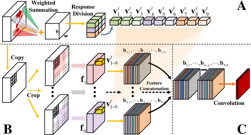
Figure 2: The reformulated network structure for our KRRCPS model. In Module B, we show two examples on how to crop the feature maps for ${\bf f}_{1}$ and ${\bf f}_{9}$. By doing this, we make the responses generated by different fragments correspond to the same input ROI region. Best viewed in high resolutions with zoom in.

3.2 Network Structure for KRRCPS

In this work, we attempt to learn ${\bm{\alpha}}_{t}$ and ${\bm{\beta}}_{t}$ by reformulating the proposed ridge regression into a neural network. This reformulation not only provides an efficient solver but also enables the algorithm to be seamlessly integrated with state-of-the-art deep feature extraction networks.

In Eq. 5, the response term ${\bf r}=\sum\limits_{m,n=1}^{M}{{\bf{f}}_{m}^{\top}{\beta_{m,n}^{t}}{{\bf{f}}_{n}}}{\bm{\alpha}}_{t}$ can be sequentially calculated by the following three steps:

$$\small\begin{array}[]{l}{\mathbf{A:}}{\kern 12.0pt}{{\bf{v}}_{n}^{t}}={{\bf{f}}_{n}}{\bm{\alpha}}_{t}\\ {\mathbf{B:}}{\kern 13.0pt}{{\bf{b}}_{m,n}}={\bf{f}}_{m}^{\top}{{\bf{v}}_{n}^{t}}\\ {\mathbf{C:}}{\kern 15.0pt}{\bf r}=\sum\limits_{m,n=1}^{M}{{\beta_{m,n}^{t}}}{{\bf{b}}_{m,n}}\end{array}.$$ (6)

Thus, we develop an equivalent neural network of our regression model (shown in Figure 2), which takes the extracted feature map as the input and outputs a heat map for target localization. This network consists of three modules, each of which precisely corresponds to one of the three operations in Eq. 6.

Module A: Given the target location, we first crop a rectangle region around the target object, and obtain the feature map ${\bf X}_{t}$ with size $H\times W\times C$, thus the target size projected on the feature map is $h\times w$. Based on the projected target size, we densely crop samples and reshape each sample to a $d$ ($=h\times w\times C$) dimensional vector. This results in a feature matrix ${\bf D}_{t}\in\mathbb{R}^{d\times N}$, based on which the output of the weighted sum layer is obtained as

$${\bf z}={\bf D}_{t}{\bm{\alpha}}_{t},$$ (7)

where ${\bf z}\in\mathbb{R}^{d\times 1}$ denotes the response for the current layer and ${\bm{\alpha}}_{t}$ is the weight vector to be learned. We reshape the vector ${\bf z}$ to a response map with size $h\times w\times C$, and then divide it into $M=\sqrt{M}\times\sqrt{M}$ sub-responses with size $(h/\sqrt{M})\times(w/\sqrt{M})\times C$. We use ${\bf v}_{1}^{t}...{\bf v}_{M}^{t}$ to denote these sub-responses in Figure 2.

Module B: This module corresponds to the second equation of Eq. 6, which is equivalent to a convolution layer. Noticing that the feature map corresponding to ${\bf f}_{m},m\in\{1,...,M\}$ is a sub-region of the input feature map ${\bf X}_{t}$ and is different when $m$ varies, we first obtain the feature map corresponding to ${\bf f}_{m}$ by cropping ${\bf X}_{t}$ (see Module B in Figure 2 for example) and feed it into a convolution layer which takes ${\bf v}_{1}^{t}...{\bf v}_{M}^{t}$ as an ensemble of filter kernels. As we have $M$ patches in total, the convolution layer has $M$ outputs, each of which has the size $(H-h+1)\times(W-w+1)\times M$.

Module C: We concatenate the $M$ outputs of Module B through the Concat layer, and input the concatenated feature maps into a convolution layer, whose kernel size is $1\times 1\times M^{2}$. This module corresponds to operation C in Eq. 6, and the filter kernel corresponds to ${\bm{\beta}}_{t}$.

In this work, we use the backpropagation algorithm to solve this network. The computational complexity for both forward and backward propagations is $\mathcal{O}(dN)$, which is much more efficient than the original solver. Note that our network is defined based on Eq. 5 for model learning. At the detection stage in frame $t$, we just need to replace ${\bf D}_{t}$, ${\bm{\alpha}}_{t}$ and ${\bm{\beta}}_{t}$ in the network with ${\bf\hat{D}}_{t}$, ${\hat{\bm{\alpha}}}_{t}$ and ${\hat{\bm{\beta}}}_{t}$ which are iteratively updated using Eq. 8 ($\eta$ is the update rate).

$$\begin{array}[]{l}{{{\bf{\hat{D}}}}_{t}}=(1-\eta){{{\bf{\hat{D}}}}_{t-1}}+\eta{{\bf{D}}_{t-1}}\\ {{\hat{\bm{\alpha}}}_{t}}=(1-\eta){{\hat{\bm{\alpha}}}_{t-1}}+\eta{{\bm{\alpha}}_{t-1}}\\ {{\hat{\bm{\beta}}}_{t}}=(1-\eta){{\hat{\bm{\beta}}}_{t}}+\eta{{\bm{\beta}}_{t-1}}\end{array}.$$ (8)

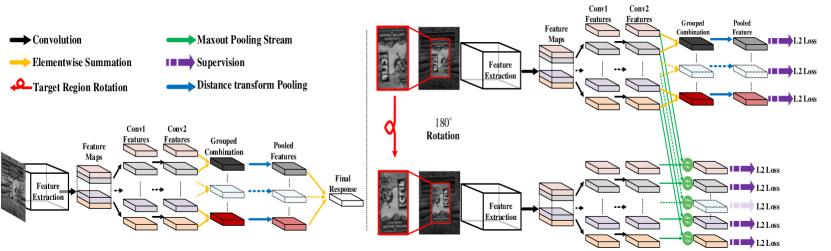
Figure 3: Network structures for our CNNSRK model. (a) The testing network for CNNSRK. We use a convolutional neural network to estimate the target position and exploit the distance transform pooling layer to determine the effectiveness of each response map. (b) The training network for CNNSRK. We utilize the two-stage training strategy to update/train the convolution and distance transform pooling layers separately. A two-stream network is used to learn the rotation information of the target. Best viewed in color with zoom in.

4 Spatial-Aware CNN

As is described in previous papers (e.g., [1, 19]), the spatial information plays an important role in a visual tracking system. However, the spatial layouts of the target object are usually ignored in the current CNN-based tracking algorithms. What is more, the existing algorithms do not perform well when the target object suffers from a severe in-plane rotation. In this work, we propose a convolution layer with spatially regularized filter kernels, through which each convolution kernel only focuses on a specific region of the target. In addition, as the training samples in visual tracking are very limited, we develop a two-stream training strategy to avoid overfitting and consider rotation information.

4.1 CNN with Spatially Regularized Kernels (CNNSRK)

The proposed CNN framework with spatially regularized kernels is illustrated in Figure 3 (a), which consists of two convolution layers interleaved with an ReLU layer and several distance transform pooling layers. Given the input feature map, we first reshape it to $46\times 46\times C$, where $C$ is the channel number. Based on the input feature map, the first convolution layer (conv1) has a kernel size of $5\times 5$, and outputs a feature map with size $46\times 46\times C_{1}$. The second convolution layer (conv2) has a kernel size of $3\times 3$ (we divide the input feature into $C_{1}$ groups), and outputs a $46\times 46\times C_{1}$ response map, each channel of which is a heat map for the target localization. After that, we divide the response map into several groups ($C_{1}/4$ groups in our implementation), and sum the responses in each group through the channel dimension, which results in a $46\times 46\times 1$ output for each group. Finally, the obtained response maps are fed into distance transform pooling layers, and the outputs are effectively combined to produce a final heat map for target localization. The detailed structure is shown in Figure 3 (a).

Convolution Layer with Spatially Regularized Filter Kernels: The target object may experience deformations and occlusions during tracking, which makes some parts of the target object more important than others. To address this issue, Wang et al. [32] modifies the implementation of the Dropout layer and keep the dropped activations fixed in the training process. By doing this, the learned convolution layers are forced to focus on different parts of the input feature map. But the discriminant ability of their model is weak as it merely takes parts of the input feature map for consideration in the training process. In this work, instead of introducing constraints on the input feature map, we enforce constraints on the filter kernels in the convolution layer. Compared with [30], our method considers the spatial information, and fixes the filter mask during the tracking process.

Let ${\bf F}_{c}\in\mathbb{R}^{K_{h}\times K_{w}\times K_{c}}$ denotes the filter kernel weights associated with the $c$-th channel of the output feature map ${\bf O}_{c}$. We introduce the spatial regularization weights ${\bf W}_{c}$ into the convolution layer, which has the same size as ${\bf F}_{c}$. By considering the spatial regularization weights, the output feature map ${\bf O}_{c}$ can be calculated as,

$${\bf O}_{c}=({\bf F}_{c}\odot{\bf W}_{c})*{\bf X}_{c}+b,$$ (9)

where $*$ denotes the convolution operation, $\odot$ stands for the Hadamard product, ${\bf X}_{c}$ represents the input feature map and $b$ is the bias term. For constructing ${\bf W}_{c}$, we first generate a binary mask ${\bf M}_{c}$ of size $K_{h}\times K_{w}$ through Bernoulli distribution $B(0.3)$ and then construct ${\bf W}_{c}$ based on this mask,

$${{\bf{W}}_{c}}(p,q,r)={{\bf{M}}_{c}}(p,q),$$ (10)

where $p$, $q$ and $r$ denote the indexes of a 3-dimensional matrix. Clearly, only parts of the spatial regions in ${\bf{W}}_{c}$ have non-zero values, which forces the filter kernels to focus on different regions.

Distance Transform Pooling Layer: The distance transform has been used in previous studies for object detection ([11, 27]). Girshick et al. [13] point out that distance transform is indeed a generalization of the max pooling layer and can be expressed in a similar formula as max pooling.

Given a function $y=f(x)$ defined on a regular grid $\mathcal{G}$, its distance transform can be calculated as,

$${D_{f}}(s)=\max_{{t\in\mathcal{G}}}(f(t)-d(s-t)).$$ (11)

Here $d(s-t)$ is a convex quadratic function with $d(s-t)=\varpi(s-t)^{2}+\theta(s-t)$, where $\varpi$ and $\theta$ are learnable parameters. The distance transform pooling layer can be used to estimate the reliability of the input feature map. Generally speaking, the larger the learned value $\varpi$ is, the more reliable the input feature map is. When $\varpi=\theta=0$, this layer outputs a response with constant values, which means that the input feature map does not influence the tracking result. In this work, the distance transform pooling layer is implemented in the Caffe framework according to [14] and the pooling region is bounded for efficient computation.

4.2 Two-Stream Training Strategy

Based on our observation that the tracking performance is inevitably influenced when severe in-plane-rotation occurs, we develop a two-stream network to learn the weights of convolution and distance transform pooling layers. The proposed two-stream network is presented in Figure 3 (b), in which the weights of the convolution layers are shared.

The upper branch of the network exploits the same feature map as the original network (Figure 3 (a)), and the lower branch uses the input feature map corresponding to the rotated target object. The previous two layers are the same as the original network, resulting in two $46\times 46\times C_{1}$ response maps in both upper and lower branches. Then, we conduct the max-out pooling operation on these two response maps to produce a $46\times 46\times C_{1}$ response. We compute the loss for each channel of the response maps and propagate the loss backward to learn the filters in convolution layers. After that, we fix the convolution layers and learn the model parameters of the distance transform pooling layers. Some visual results are illustrated in Figure 4, from which we can see that the proposed two-stream training strategy facilitates dealing with severe in-plane rotation.

In addition, the reason why we do not directly perform model learning on the original network (presented in Figure 3 (a)) is to avoid the overfitting problem. For example, the original network has a total of $5\times 5\times C\times C_{1}+3\times 3\times C_{1}+C_{1}$ parameters. If $C=512$ and $C_{1}=100$, there will be a total of 1281000 parameters, which are very difficult to be learned with limited training data in visual tracking. The proposed two-stream strategy essentially decomposes the network into several sub-parts and trains each part separately, thereby facilitating avoiding overfitting.

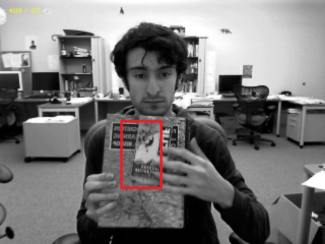
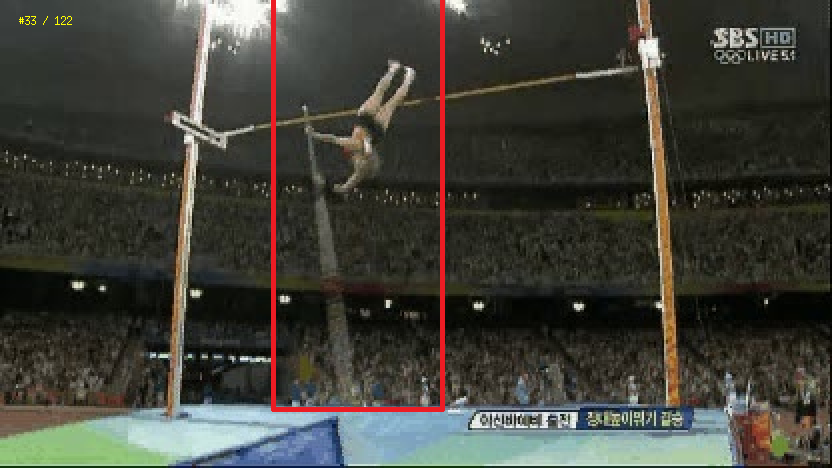
(a)	(b)

Figure 4: Tracking results with and without two-stream training process are illustrated in (a) and (b), respectively. We can see that the proposed two-stream training strategy makes the tracker perform better when severe in-plane rotation occurs.

5 Tracking with Spatial-Aware KRR and CNN

In this section, we describe how to exploit both spatial-aware KRR and CNN models for robust visual tracking.

5.1 Target Location Estimation

We conduct visual tracking by combining the responses of our KRR and CNN models. The former one captures the holistic information of the target, while the latter one focuses more on the localized region. In frame $t$, we crop a search region centered by the estimated object location of the last frame and then obtain a feature map ${\bf X}_{t}$ for this region. Furthermore, the final heat map of our tracker can be computed as,

$${\bf f}({{\bf{X}}_{t}})={{\bf f}_{KRR}}({{\bf{X}}_{t}})+\gamma{{\bf f}_{CNN}}({{\bf{X}}_{t}}),$$ (12)

where $\gamma$ is a trade-off parameter. ${{\bf f}_{KRR}}({{\bf{X}}_{t}})$ and ${{\bf f}_{CNN}}({{\bf{X}}_{t}})$ denote the heat maps produced by KRR and CNN models, respectively. Finally, we find the position with highest heat map score in ${\bf f}({{\bf{X}}_{t}})$ and determine it as the optimal location.

5.2 Scale Estimation

It is not enough to only provide the location for a target object, which may experience drastic scale variation. In this work, we also estimate the scale variation of the target after location estimation. We use $S$ to denote the candidate scale size and $H\times W$ to denote the input feature map size. For each ${s_{l}}\in\left\{{\left\lfloor{-\frac{{S-1}}{2}}\right\rfloor,...,\left\lfloor{\frac{{S-1}}{2}}\right\rfloor}\right\}$, we crop or pad the input feature map to size $a^{s_{l}}H\times a^{s_{l}}W$ and reshape it to $H\times W$ (we use ${\cal T}({\bf X}_{t},s_{l})$ to denote the transformed feature map for scale $l$). These transformed maps are then fed into a fully connected layer to output the scale scores. Finally, we choose the scale related to the largest score as the optimal state. After scale estimation, we further exploit the bounding box regression method [12, 25] to refine the tracking result.

5.3 Model Update

After obtaining the optimal location and scale, we crop the corresponding search region and extract its feature map ${\bf X}_{t}$. Then, we generate an ideal heat map of Gaussian distribution [17] and exploit the L2 loss function for finetuning both KRR and CNN models to fit the ideal heat map. In this work, the stochastic gradient descent (SGD) method is adopted for finetuning both networks. For KRR, after model parameters ${\bm{\alpha}}_{t}$ and ${\bm{\beta}}_{t}$ are updated, we further update ${\bf\hat{D}}_{t}$, ${\hat{\bm{\alpha}}}_{t}$ and ${\hat{\bm{\beta}}}_{t}$ based on Eq. 8 . For CNN, our two-stream network (Section 4.2) is adopted for updating model parameters.

In addition, if scale variation is detected, we update the scale estimation network with the loss function ${{\cal L}_{\cal S}}=\frac{1}{2}\left\|{{y}_{s_{l}}-{\bf{f}}_{\cal S}({\cal T}({{\bf{X}}_{t}},{s_{l}}))}\right\|_{2}^{2}$ (${\bf{f}}_{\cal S}$ denotes the score obtained by the network, ${y_{{s_{l}}}}=\exp(-\frac{1}{{2{\sigma^{2}}}}s_{l}^{2})$ is a Gaussian function).

6 Experimental Results

In this section, we first introduce the experimental setups, and then report the experimental results of different trackers on the OTB-2015 and VOT-2017 public datasets. In addition, we verify the effectiveness of different components of the proposed method. Our source codes can be downloaded at https://github.com/cswaynecool/LSART.

6.1 Implementation Details

The proposed tracker is implemented with MATLAB2014a on an Intel 4.0 GHz CPU with 32G memory, and runs at around 1fps during online tracking. We use the Caffe toolbox [18] to implement the networks, whose forward and backward operations are conducted on a Nvidia Titan X GPU. We divide the target into 9 ($3\times 3$) patches in the kernelized ridge regression model. The trade-off parameters $\lambda_{1}$, $\lambda_{2}$ are set as 0.001 and 0.001 respectively. The learning rate $\eta$ is set as $0.2$ in the first ten frames, and changed to a smaller learning rate (e.g. $0.001$) during the tracking process. All the networks are trained with the SGD method, and the learning rates for ${\bm{\alpha}}_{t}$ and ${\bm{\beta}}_{t}$ in the KRR network are set as 8e-9 and 1.6, while the learning rate for each layer in the CNN network is fixed as 8e-7.

6.2 OTB-2015 Dataset

The OTB-2015 dataset [34] is one of the most commonly used benchmarks in evaluating different trackers. This dataset includes $100$ challenging image sequences with 11 different attributes, such as illumination variation, background clutter, scale variation, fast motion, in-plane rotation and so on. In this dataset, we exploit the the output of the Conv4-3 layer of the VGG-16 net as the basic feature for our tracker, and compare our LSART method with 12 state-of-the-art trackers including DSST [6], ECO [5], CCOT [10], SRDCF [8], KCF [17], DeepSRDCF [7], CF2 [23], LCT [24], SRDCFdecon [9], HDT [26], Staple [2] and MEEM [35]. We exploit the one-pass evaluation (OPE) for all the trackers and report both the precision and success plots for comparison. The precision plots aim to measure the percentage of frames in which the distance between the tracked result and the ground-truth is under a threshold, while the success plots aim to measure the successfully tracked frames with various thresholds. Following [33], in the precision plots, we use the distance precision rate at threshold 20 for ranking, while in the success plots, we use the area under curve (AUC) for ranking.

Figure 5 illustrates both precision and success plots over all $100$ videos in this dataset. We can see that our LSART method achieves the best performance with a precision score $92.3\%$ and the second best result with an AUC score of $67.2\%$. Overall, in OTB-2015, our tracker has comparable performance compared to the existing best tracker ECO.

Besides, we evaluate different trackers using 8 attributes and report their precision plots in Figure 6. The results show that our tracker achieves very promising performance in handling most of the challenges, especially for deformation and in-plane rotation. First, the proposed LSART method improves the second best one by 4.3% in the attribute of deformation. This improvement is mainly because that our tracker determines the reliability of the target object adaptively and is insusceptible to the unreliable regions. In addition, for in-plane rotation, our method improves the ECO method by 1.8%. The underlying reason is that our tracker exploits the two-stream network to learn the rotation information of the target object effectively.

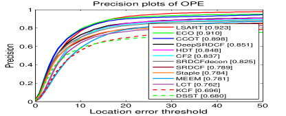
Figure 5: Precision and success plots on the OTB-2015 dataset in terms of OPE rule. In the legend, we show the distance precision rates at threshold 20 and area under curve (AUC) scores, based on which different trackers are ranked.

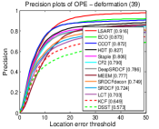
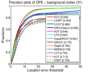
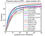
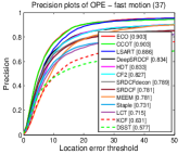
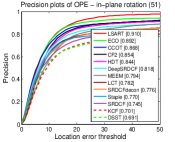
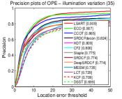
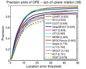
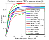
Figure 6: Performance evaluation on different attributes of OTB-2015 in terms of the OPE criterion. The reported attributes include deformation, background clutter, scale variation, fast motion, in-plane rotation, illumination variation, out-of-plane rotation, low resolution.

Table 1: Performance evaluation for 12 state-of-the-art algorithms on the VOT-2017 public dataset. The best three results are marked in red, blue and green bold fonts respectively.

Tracker	EAO	A	R	AO
LSART	0.323	0.493	0.218	0.437
CFCF	0.286	0.509	0.281	0.380
ECO	0.280	0.483	0.276	0.402
CCOT	0.267	0.494	0.318	0.390
MCPF	0.248	0.510	0.427	0.443
CRT	0.244	0.463	0.337	0.370
ECOhc	0.238	0.494	0.435	0.335
MEEM	0.192	0.463	0.534	0.328
FSTC	0.188	0.480	0.534	0.334
Staple	0.169	0.530	0.688	0.335
KCF	0.135	0.447	0.773	0.267
SRDCF	0.119	0.490	0.974	0.246

6.3 VOT-2017 Public Dataset

For more thorough evaluations, we test our LSART tracker on the VOT-2017 public dataset [20] in comparison with 11 state-of-the-art methods, including ECO [5], CCOT [10], CFCF [15], MCPF [36], CRT [4], ECOhc [5], MEEM [35], FSTC [31], Staple [2], KCF [17] and SRDCF [8]. Since many top-ranked trackers (e.g. CFCF, ECO and CCOT) exploit a combination of CNN and hand-crafted features, we extend our feature set with HOG and Color Naming like CCOT in this dataset. The VOT-2017 public dataset is one of the most recent datasets for evaluating online model-free single-object trackers, and includes $60$ public image sequences with different challenging factors. Following the evaluation protocol of VOT-2017 [20], we adopt the expected average overlap (EAO), accuracy and robustness raw values (A, R) and no-reset-based average overlap (AO) to compare different trackers. The detailed comparisons are reported in Table LABEL:tab:vot-2017.

From Table LABEL:tab:vot-2017, we can conclude that the proposed LSART method achieves the top-ranked performance in terms of EAO, R and AO criteria while maintaining a competitive accuracy. Especially, our LSART tracker has the best performance among the compared trackers in terms of the EAO measure, which is the most important metric on the VOT dataset. Compared with the second best tracker (CFCF), the proposed method achieves a relative performance gain of 12.94%. In addition, our tracker achieves a substantial improvement over the popular ECO method, with a relative gain of 15.36% in EAO. Note that our tracker has an EAO of 0.275 without the hand-crafted features, which still outperforms CCOT and is competitive among the compared trackers. The OPE rule is also adopted to evaluate different trackers and the AO values are reported to demonstrate their performance. From the last column in Table LABEL:tab:vot-2017, we can see that our method achieves comparable performance compared to the MCPF tracker and improves the ECO method by a relative gain of 8.71%.

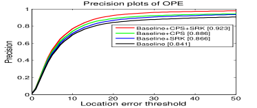
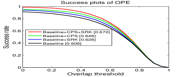
Figure 7: Performance evaluation for each component of the proposed tracker.

6.4 Ablation Studies

In this paper, we propose two complementary spatial aware regressions for visual tracking, which are respectively the kernelized ridge regression model with cross-patch similarity and convolution neural network with the spatially regularized kernels. Here, we conduct ablation analysis to evaluate each component of our tracker. With different experimental settings, we obtain the following 4 variants of our tracker, which are respectively named as “Baseline”, “Baseline+CPS”, “Baseline+SRK” and “Baseline+CPS+SRK” (LSART). We use the shorthand “Baseline” to denote the method that directly combines the conventional KRR and CNN models, and adopt the abbreviations “CPS”, “SRK” to denote the cross-patch similarity kernel and spatial regularized filter kernel. Using OTB-2015, the results of different variants are presented in Figure 7.

First, the direct combination of conventional KRR and CNN models (i.e., “Baseline”) cannot achieve satisfactory performance ($0.841$ in precision score and $0.606$ in AUC score). Second, the effectiveness of the CPS module can be verified comparing“Baseline+CPS” with “Baseline”, which contributes to the relative performance gains of $5.35\%$ and $6.93\%$ in precision and success plots. The effectiveness of the SRK module can be validated by comparing “Baseline+SRK” with “Baseline”. Finally, we can see that our LSART method (“Baseline+CPS+SRK”) improves the original “Baseline” method by relative gains of $9.75\%$ in precision plots and $10.89\%$ in success plots.

7 Conclusion

This paper proposes a robust online tracker by exploiting both spatial-aware KRR and spatial-aware CNN. First, we propose a novel KRR model with cross-patch similarity (CPS). This model considers the interior structure of the target, and can adaptively determine the importance of the similarity score between two patches. We show that the KRRCPS model can be reformulated as a neural network, and thus can be more efficiently solved. In addition, we propose a complementary CNN model which focuses more on the localized region via a spatially regularized filter kernel. Distance transform pooling layers are further exploited to determine the reliability of the convolutional layers. Finally, the above-mentioned two models are effectively combined to generate a final heat map for target location. Experimental results on two recent benchmarks demonstrate that the proposed LSART method achieves very promising tracking performance, especially on the VOT-2017 public dataset.

Acknowledgment. This paper is partially supported by the Natural Science Foundation of China #61725202, #61502070, #61472060, NSF CAREER (No. 1149783), gifts from Adobe, Toyota, Panasonic, Samsung, NEC, Verisk and Nvidia. Chong Sun is also supported by the China Scholarship Council (CSC).

References

- [1] A. Adam, E. Rivlin, and I. Shimshoni. Robust fragments-based tracking using the integral histogram. In CVPR, 2006.
- [2] L. Bertinetto, J. Valmadre, S. Golodetz, O. Miksik, and P. H. Torr. Staple: Complementary learners for real-time tracking. In CVPR, 2016.
- [3] D. S. Bolme, J. R. Beveridge, B. A. Draper, and Y. M. Lui. Visual object tracking using adaptive correlation filters. In CVPR, 2010.
- [4] K. Chen and W. Tao. Convolutional regression for visual tracking. arXiv preprint arXiv:1611.04215, 2016.
- [5] M. Danelljan, G. Bhat, F. S. Khan, and M. Felsberg. Eco: Efficient convolution operators for tracking. In CVPR, 2017.
- [6] M. Danelljan, G. Häger, F. Khan, and M. Felsberg. Accurate scale estimation for robust visual tracking. In BMVC, 2014.
- [7] M. Danelljan, G. Hager, F. Shahbaz Khan, and M. Felsberg. Convolutional features for correlation filter based visual tracking. In ICCV Workshops, 2015.
- [8] M. Danelljan, G. Hager, F. Shahbaz Khan, and M. Felsberg. Learning spatially regularized correlation filters for visual tracking. In ICCV, 2015.
- [9] M. Danelljan, G. Hager, F. Shahbaz Khan, and M. Felsberg. Adaptive decontamination of the training set: A unified formulation for discriminative visual tracking. In CVPR, 2016.
- [10] M. Danelljan, A. Robinson, F. S. Khan, and M. Felsberg. Beyond correlation filters: Learning continuous convolution operators for visual tracking. In ECCV, 2016.
- [11] P. F. Felzenszwalb, R. B. Girshick, D. McAllester, and D. Ramanan. Object detection with discriminatively trained part-based models. IEEE Transactions on Pattern Analysis and Machine Intelligence, 32(9):1627–1645, 2010.
- [12] R. Girshick, J. Donahue, T. Darrell, and J. Malik. Rich feature hierarchies for accurate object detection and semantic segmentation. In CVPR, 2014.
- [13] R. Girshick, F. Iandola, T. Darrell, and J. Malik. Deformable part models are convolutional neural networks. In CVPR, 2015.
- [14] I. J. Goodfellow, D. Warde-Farley, M. Mirza, A. C. Courville, and Y. Bengio. Maxout networks. Journal of Machine Learning Research, 28:1319–1327, 2013.
- [15] E. Gundogdu and A. A. Alatan. Good features to correlate for visual tracking. arXiv preprint arXiv:1704.06326, 2017.
- [16] J. F. Henriques, R. Caseiro, P. Martins, and J. Batista. Exploiting the circulant structure of tracking-by-detection with kernels. In ECCV, 2012.
- [17] J. F. Henriques, R. Caseiro, P. Martins, and J. Batista. High-speed tracking with kernelized correlation filters. IEEE Transactions on Pattern Analysis and Machine Intelligence, 37(3):583–596, 2015.
- [18] Y. Jia, E. Shelhamer, J. Donahue, S. Karayev, J. Long, R. Girshick, S. Guadarrama, and T. Darrell. Caffe: Convolutional architecture for fast feature embedding. In ICMM, 2014.
- [19] H.-U. Kim, D.-Y. Lee, J.-Y. Sim, and C.-S. Kim. Sowp: Spatially ordered and weighted patch descriptor for visual tracking. In ICCV, 2015.
- [20] M. Kristan, A. Leonardis, J. Matas, M. Felsberg, R. Pflugfelder, L. Zajc, T. Vojir, and G. Hager. The visual object tracking vot2017 challenge results. In ICCV Workshops, 2017.
- [21] H. Li, Y. Li, and F. Porikli. Robust online visual tracking with a single convolutional neural network. In ACCV, 2014.
- [22] P. Li, D. Wang, L. Wang, and H. Lu. Deep visual tracking: Review and experimental comparison. Pattern Recognition, 76:323–338, 2018.
- [23] C. Ma, J.-B. Huang, X. Yang, and M.-H. Yang. Hierarchical convolutional features for visual tracking. In ICCV, 2015.
- [24] C. Ma, X. Yang, C. Zhang, and M.-H. Yang. Long-term correlation tracking. In CVPR, 2015.
- [25] H. Nam and B. Han. Learning multi-domain convolutional neural networks for visual tracking. In CVPR, 2016.
- [26] Y. Qi, S. Zhang, L. Qin, H. Yao, Q. Huang, J. Lim, and M.-H. Yang. Hedged deep tracking. In CVPR, 2016.
- [27] P.-A. Savalle, S. Tsogkas, G. Papandreou, and I. Kokkinos. Deformable part models with cnn features. In ECCV Workshop, 2014.
- [28] B. Scholkopf, R. Herbrich, A. J. Smola, and R. Williamson. A generalized representer theorem. In COLT, 2001.
- [29] R. Tao, E. Gavves, and A. W. Smeulders. Siamese instance search for tracking. In CVPR, 2016.
- [30] L. Wan, M. Zeiler, S. Zhang, Y. Le Cun, and R. Fergus. Regularization of neural networks using dropconnect. In ICML, 2013.
- [31] L. Wang, W. Ouyang, X. Wang, and H. Lu. Visual tracking with fully convolutional networks. In CVPR, 2015.
- [32] L. Wang, W. Ouyang, X. Wang, and H. Lu. Stct: Sequentially training convolutional networks for visual tracking. In CVPR, 2016.
- [33] Y. Wu, J. Lim, and M.-H. Yang. Online object tracking: A benchmark. In CVPR, 2013.
- [34] Y. Wu, J. Lim, and M.-H. Yang. Object tracking benchmark. IEEE Transactions on Pattern Analysis and Machine Intelligence, 37(9):1834–1848, 2015.
- [35] J. Zhang, S. Ma, and S. Sclaroff. Meem: robust tracking via multiple experts using entropy minimization. In ECCV, 2014.
- [36] T. Zhang, C. Xu, and M.-H. Yang. Multi-task correlation particle filter for robust object tracking. In CVPR, 2017.