A mid-infrared statistical investigation of clumpy torus model predictions

Abstract

We present new calculations of the CAT3D clumpy torus models, which now include a more physical dust sublimation model as well as AGN anisotropic emission. These new models allow graphite grains to persist at temperatures higher than the silicate dust sublimation temperature. This produces stronger near-infrared emission and bluer mid-infrared (MIR) spectral slopes. We make a statistical comparison of the CAT3D model MIR predictions with a compilation of sub-arcsecond resolution ground-based MIR spectroscopy of 52 nearby Seyfert galaxies (median distance of 36 Mpc) and 10 quasars. We focus on the AGN MIR spectral index $\alpha_{\rm MIR}$ and the strength of the $9.7\,\mu$m silicate feature $S_{\rm Sil}$. As with other clumpy torus models, the new CAT3D models do not reproduce the Seyfert galaxies with deep silicate absorption ($S_{\rm Sil}<-1$). Excluding those, we conclude that the new CAT3D models are in better agreement with the observed $\alpha_{\rm MIR}$ and $S_{\rm Sil}$ of Seyfert galaxies and quasars. We find that Seyfert 2 are reproduced with models with low photon escape probabilities, while the quasars and the Seyfert 1-1.5 require generally models with higher photon escape probabilities. Quasars and Seyfert 1-1.5 tend to show steeper radial cloud distributions and fewer clouds along an equatorial line-of-sight than Seyfert 2. Introducing AGN anisotropic emission besides the more physical dust sublimation models alleviates the problem of requiring inverted radial cloud distributions (i.e., more clouds towards the outer parts of the torus) to explain the MIR spectral indices of type 2 Seyferts.

1 Introduction

The dusty molecular torus is a key component of the Unification Model (Antonucci, 1993; Urry & Padovani, 1995) of Active Galactic Nuclei (AGN). Since the torus was first proposed to explain the detection of polarised broad lines in NGC 1068 and radio galaxies (Antonucci, 1984) until its first direct detection with ALMA in NGC1068 (García-Burillo et al., 2016; Gallimore et al., 2016), our view of the torus has evolved enormously.

Table 1: Summary of sample properties.

Name	z	$D_{\rm L}$	Morphological	$b/a$	Activity	Ref. Activity
		(Mpc)	type		type	type
Circinus	0.001448	4.2	SA(s)b?	0.4	Sy 2	f
ESO 103-G35	0.013286	59.1	S0?	0.4	Sy 2	j, k, l
ESO 323-G077	0.015014	60.2	(R)SAB0^0(rs)	0.7	Sy 1.2	k, l
ESO 428-G14	0.005664	23.3	SAB0^0(r) pec	0.6	Sy 2	l
IC 4329A	0.016054	79.8	SA0^ edge-on	0.3	Sy 1.2	j, k, l
IC 4518W	0.016261	79.2	Sc pec	0.5	Sy 2	k, l
IC 5063	0.011348	49.9	SA0^+(s)?	0.7	Sy 2	j, k
MGC-3-34-64	0.016541	78.8	S0/a	0.8	Sy 1.8	j, k
MGC-5-23-16	0.008486	35.8	S0?	0.5	Sy 2	j, k
MCG-6-30-15	0.007749	26.8	S?	0.6	Sy 1.2	j, k
Mrk 3	0.013509	58.5	S0?	0.9	Sy 2	j, k
Mrk 1066	0.012025	49.0	(R)SB0^+(s)	0.6	Sy 2	l
Mrk 1210	0.013496	58.9	S?	1.0	Sy 2	l
Mrk 1239	0.019927	88.9	E-S0	1.0	Sy 1.5	h
NGC 931	0.016652	67.5	SAbc	0.2	Sy 1.5	j, k
NGC 1068	0.003793	15.2	(R)SA(rs)b	0.9	Sy 2	k
NGC 1194	0.013596	54.5	SA0^+?	0.6	Sy 1.9	l
NGC 1320	0.008883	35.5	Sa? edge-on	0.3	Sy 2 l
NGC 1365	0.005457	21.5	SB(s)b	0.6	Sy 1.5	i
NGC 1386	0.002895	10.6	SB0^+(s)	0.4	Sy 2	f
NGC 1808	0.003319	12.3	(R)SAB(s)a	0.6	Sy 2	b
NGC 2110	0.007789	32.4	SAB0^-	0.8	Sy 2	j, k
NGC 2273	0.006138	28.7	SB(r)a?	0.8	Sy 2	c
NGC 2992	0.007710	34.4	Sa pec	0.3	Sy 1.9	l
NGC 3081	0.007976	34.5	(R)SAB0/a(r)	0.8	Sy 2	j, k
NGC 3094	0.008019	38.3	SB(s)a	0.7	Sy 2	a
NGC 3227	0.003859	20.4	SAB(s)a pec	0.7	Sy 1.5	j, k, l
NGC 3281	0.010674	45.0	SA(s)ab pec?	0.5	Sy 2	j, k, l
NGC 3783	0.009730	36.4	(R’)SB(r)ab	0.9	Sy 1	j, k
NGC 4051	0.002336	12.9	SAB(rs)bc	0.7	Sy 1.5	j, k
NGC 4151	0.003319	20.0	(R’)SAB(rs)ab?	0.7	Sy 1.5	j, k, l
NGC 4253	0.012929	61.3	(R’)SB(s)a?	0.8	Sy 1.5	j
NGC 4258	0.001494	7.98	SAB(s)bc	0.4	Sy 1.9	d
NGC 4388	0.008419	17.0	SA(s)b? edge-on	0.2	Sy 2	j, k
NGC 4418	0.007268	34.9	(R’)SAB(s)a	0.5	Sy 2	l
NGC 4507	0.011801	60.2	(R’)SAB(rs)b	0.8	Sy 2	j, k
NGC 4579	0.00506	17.0	SAB(rs)bc	0.8	Sy 1.9	d
NGC 4593	0.009000	41.6	(R)SB(rs)b	0.7	Sy 1	j, k, l
NGC 5135	0.013693	58.3	SB(s)ab	0.7	Sy 2	l
NGC 5347	0.007789	40.2	(R’)SB(rs)ab	0.8	Sy 2	l
NGC 5506	0.006181	30.1	Sa pec edge-on	0.2	Sy 1.9	j, k
NGC 5548	0.017175	80.3	(R’)SA0/a(s)	0.9	Sy 1.5	j, k, l
NGC 5643	0.003999	14.4	SAB(rs)c	0.9	Sy 2	l
NGC 5995	0.025194	115	S(B)c	0.9	Sy 2	k
NGC 7130	0.016151	69.6	Sa pec	0.9	Sy 2	f
NGC 7172	0.008683	37.9	Sa pec edge-on	0.6	Sy 2	j, k, l
NGC 7213	0.005839	25.1	SA(s)a?	0.9	Sy 1.5	j, k
NGC 7465	0.006538	28.4	(R’)SB0^0?(s)	0.7	Sy 2	e
NGC 7469	0.016317	67.9	(R’)SAB(rs)ab?	0.7	Sy 1.2	j, k
NGC 7479	0.007942	33.9	SB(s)c	0.8	Sy 1.9	l
NGC 7582	0.005254	22.1	(R’)SB(s)ab	0.4	Sy 2	j, k
NGC 7674	0.028924	120	SA(r)bc pec	0.9	Sy 2	g

Notes.— For each galaxy we give its redshift, luminosity distance ($D_{\rm L}$), morphological type, the axis ratio ($b/a$), and the optical activity type. References.— ^aAsmus et al. (2014); ^bBrightman & Nandra (2011); ^cContini et al. (1998); ^dMaiolino & Rieke (1995); ^eMalizia et al. (2012); ^fMarinucci et al. (2012); ^gOsterbrock & Martel (1993); ^hPolletta et al. (1996); ⁱSchulz et al. (1999); ^jTueller et al. (2008); ^kTueller et al. (2010); ^lVéron-Cetty & Véron (2010).

From an observational point of view, high angular resolution near and mid-infrared (NIR and MIR, respectively) imaging and spectroscopy are now routinely isolating the unresolved emission believed to be associated with dust heated by the AGN and in particular with dust in the torus (Mason et al., 2006; Ramos Almeida et al., 2009, 2011; Alonso-Herrero et al., 2011; Asmus et al., 2014; García-Bernete et al., 2016). The modelling of MIR interferometric observations infers a compact central obscuring source with a size typically of less than approximately 10 pc (MIR half-light radii, see Tristram et al., 2009; Burtscher et al., 2013). However, some recent findings are starting to complicate this simple scenario of the torus as an isolated structure. For instance, some Seyfert galaxies show a large fraction of the nuclear dust emission in the polar direction (Hönig et al., 2013; López-Gonzaga et al., 2016). Also, it is clear that in many AGN there are nuclear extended dust components (e.g., dust lanes, dust in the narrow line region and/or ionisation cones) not necessarily associated with the dusty torus (see e.g., Radomski et al., 2003; Packham et al., 2005b; Mason et al., 2006; Roche et al., 2006; Roche et al., 2007; Alonso-Herrero et al., 2011; Asmus et al., 2016; García-Bernete et al., 2016).

Torus models are also quickly improving. The early models had the dust uniformly distributed (Pier & Krolik, 1992; Granato & Danese, 1994; Stenholm, 1994; Efstathiou & Rowan-Robinson, 1995; Manske & Henning, 1998; van Bemmel & Dullemond, 2003; Schartmann et al., 2005; Fritz et al., 2006; Feltre et al., 2012) mostly due to computational reasons. However, it was understood that the obscuring material in the torus had to be in clouds because otherwise it would be very difficult for the dust to survive in this region (Krolik & Begelman, 1988). For more than a decade now, the majority of torus models adopt a clumpy distribution for the dust (see e.g., Rowan-Robinson, 1995; Nenkova et al., 2002, 2008a, 2008b; Dullemond & van Bemmel, 2005; Hönig et al., 2006; Schartmann et al., 2008; Hönig & Kishimoto, 2010; Stalevski et al., 2016). The newest models now include a more realistic representation of the torus by having a clumpy two-phase medium (Stalevski et al., 2012; Siebenmorgen et al., 2015) and a clumpy dusty torus with a polar outflow (Hönig & Kishimoto, 2017). Other models have radiation-driven obscuring structures which replace the classical torus (see e.g., Wada, 2012).

Clumpy torus models fit reasonably well the unresolved nuclear infrared emission of local AGN (Ramos Almeida et al., 2009; Hönig et al., 2010; Ramos Almeida et al., 2011; Alonso-Herrero et al., 2011; Sales et al., 2011; Lira et al., 2013; Ichikawa et al., 2015; Siebenmorgen et al., 2015; Audibert et al., 2017). However, in some cases fitting the entire nuclear infrared range simultaneously with clumpy torus models alone can be challenging (see e.g., Mor et al., 2009; García-Burillo et al., 2016; Martínez-Paredes et al., 2017). Thus, there is still room for improvement. In this work we present new calculations of the Hönig & Kishimoto (2010) torus models, known as CAT3D models. We focus on two different improvements, namely, a more physical description of the dust sublimation model and the inclusion of AGN anisotropic emission. Both possibilities were discussed by Kishimoto et al. (2007) to explain the K-band interferometric observations of type 1 Seyferts. As we shall see, this more physically motivated dust sublimation model allows for the graphites grains to survive at higher temperatures than usually assumed for the silicates. This may alleviate the problem of the excess of nuclear NIR emission with respect to the current clumpy torus predictions found mostly for type 1 AGN (Mor et al., 2009; Alonso-Herrero et al., 2011; Ichikawa et al., 2015) but also type 2 AGN (Lira et al., 2013). Indeed, Mor et al. (2009) and Mor & Netzer (2012) included a hot dust graphite component in addition to the standard torus to model the infrared SEDs of type 1 AGN. Finally, with the availability of large samples of Seyfert galaxies with sub-arcsecond resolution MIR spectroscopy (Hönig et al., 2010; González-Martín et al., 2013; Alonso-Herrero et al., 2016a), we can also compare the CAT3D torus old and new model predictions for the MIR nuclear emission with AGN observations taking a more statistical approach.

This paper is organized as follows. Section 2 describes the compilation of MIR spectroscopy used in this work and Section 3 the MIR properties of the AGN emission as derived using a spectral decomposition method. Section 4 presents the new CAT3D torus model calculations, as well as a comparison with the previous version of the model and the MIR observations. We summarize our conclusions in Section 5.

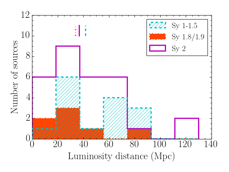
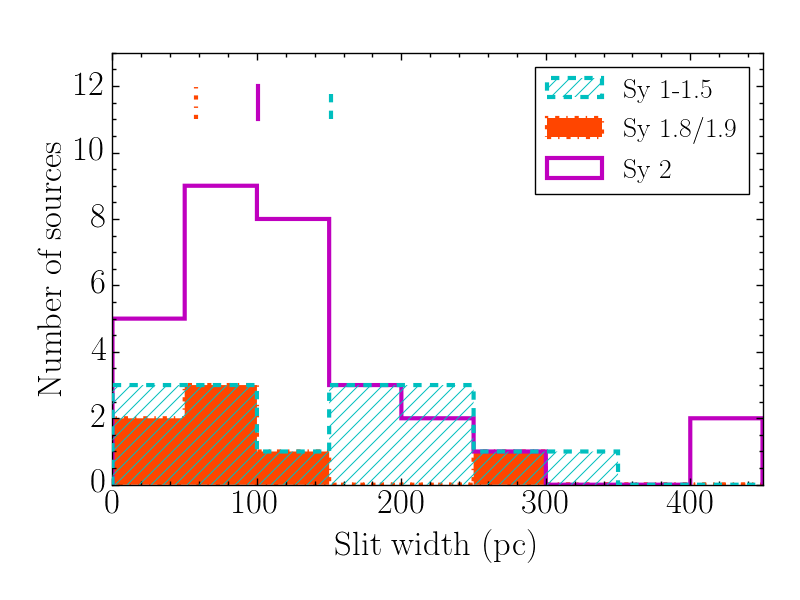
Figure 1: Distribution of the luminosity distance (left) and the slit width (right) for the Seyfert 2 galaxies (30, magenta histograms), Seyfert 1-1.5 galaxies (15, hatched cyan histograms), and Seyfert 1.8/1.9 (7, filled orange histograms). The vertical lines indicate the corresponding median values of the distributions.

2 Sample and MIR ground based observations

We compiled a sample of 52 Seyfert galaxies (see Table 1) with existing high angular resolution MIR spectroscopy (Table 2) obtained on $8-10\,$m class telescopes. We chose instruments on large telescopes to take advantage of the angular resolutions typically achieved in the MIR, $0.3-0.4$ arcsec. This allows us to probe the nuclear regions of Seyfert galaxies with angular resolutions almost a factor of ten better than with the Spitzer Infrared Spectrograph (IRS, Houck et al., 2004). We used observations taken with four different instruments covering the $N$-band atmospheric window, approximately between 7.5 and 13.5 $\mu$m. The instruments include the Thermal-Region Camera Spectrograph (T-ReCS; Telesco et al. 1998) on the 8.1 m Gemini-South Telescope, the Very Large Telescope (VLT) spectrometer and imager for the mid-infrared (VISIR; Lagage et al. 2004) on the 8.2 m VLT UT3 telescope at ESO/Paranal observatory, the CanariCam instrument (Telesco et al., 2003; Packham et al., 2005a) on the 10.4 m Gran Telescopio CANARIAS (GTC) in El Roque de los Muchachos Observatory, and Michelle (Glasse et al., 1997) on the 8.1 m Gemini-North Telescope. The CanariCam spectroscopy was taken as part of the ESO/GTC large programme 182.B-2005 (PI Alonso-Herrero).

Table 1 summarizes the properties of the Seyfert galaxies in our sample including their redshift, luminosity distance ($H_{0}=73\,{\rm km\,s}^{-1}\,{\rm Mpc}^{-1}$, $\Omega_{M}=0.27$ and $\Omega_{\Lambda}=0.73$), morphological type, the axis ratio ($b/a$), and the optical activity type (see below). We used the luminosity distance obtained from the NASA Extragalactic Database (NED) using the corrected redshift to the reference frame defined by the Virgo cluster, the Great Attractor and the Shapley supercluster. We obtained the spectral classification of our galaxies from the literature (see last column of Table 1 for the references). We grouped together all Seyferts going from Seyfert 1 to Seyfert 1.5 and those classified as Seyfert 1.8 and Seyfert 1.9. This resulted in 15 galaxies in the Seyfert 1-1.5 group, 7 in the Seyfert 1.8/1.9, and 30 in the Seyfert 2 group. In Fig. 1 (left panel) we show the luminosity distance distributions for the Seyfert 2, Seyfert 1.8/1.9, and Seyfert 1-1.5. The distances of the different type Seyfert galaxies are similar (median value of 36.1 Mpc), although the Seyfert 1-1.5 galaxies are slightly further away (median of 42 Mpc) than the Seyfert 2 galaxies (median of 37 Mpc) in our sample.

We obtained the ground-based high angular resolution MIR spectroscopy from several works (mostly from Hönig et al., 2010; González-Martín et al., 2013; Esquej et al., 2014; Alonso-Herrero et al., 2016a, but see the last column of Table 2 for a complete list of references). In Table 2 for each galaxy in the sample we summarize some of the observational details of the MIR spectroscopy, namely, the instrument, the slit width (in arcsec and pc, respectively), and the reference to the published spectra. Out of the 52 galaxies, 17 were observed with CanariCam, 18 with T-ReCS, 23 with VISIR, and 1 with Michelle. As can be seen from this table, 7 galaxies in our sample were observed with two different instruments. For those cases, in Section 3.1 and the Appendix we will discuss in detail which one is used for the analysis. As can also be seen from this table, the slit widths for the different instruments vary between 0.35 arcsec and 0.75 arcsec, which are appropriate for the image quality values (FWHM) of the observations in the MIR (typically $\leq 0.4\,$arcsec, see e.g., Hönig et al. 2010 and Alonso-Herrero et al. 2016a). For the distances of our Seyfert galaxies, the slits probe nuclear regions between 7 and 436 pc, with a median value of 101 pc for the entire sample. Finally, we used for this work the fully reduced and calibrated 1-dimensional spectra of the galaxies. We refer the reader to the original articles (see Table 2) for details of the observations and data reduction. In Fig. 1 (right panel) we show the slit width (in parsec) distributions for the Seyfert 2, Seyfert 1-1.5, and Seyfert 1.8/1.9 in our sample. The median of the slit width is larger for the Seyfert 1-1.5 galaxies (median physical sizes of 151 pc) than the Seyfert 2 (101 pc), as expected because the former are more distant on average.

Our sample of Seyfert galaxies is by necessity flux-limited in the MIR so high signal-to-noise ratio MIR spectroscopy could be obtained with reasonable integration times. Typically these MIR fluxes within small apertures are above 20 mJy and the acquisition of the target also requires relatively compact morphologies (see for instance Alonso-Herrero et al. 2016a for a more detailed discussion). This results in typical AGN luminosities at rest-frame $12\,\mu$m in the range $\log\nu L_{\nu}(12\mu{\rm m})\sim 42-44\,{\rm erg\,s}^{-1}$ (see Hönig et al., 2010; Alonso-Herrero et al., 2016a, and also Section 3). Although not a complete sample, it is likely to be representative of the galaxies at the median distance of the sample. For instance, it contains 80% of the Seyferts in the complete volume-limited sample (distances between 10 and 40 Mpc) selected from the nine-month Swift-BAT catalogue at $14-195\,$keV (Tueller et al., 2008) analysed by García-Bernete et al. (2016).

Table 2: Summary of MIR spectroscopic observations

Name	Instrument	slit width (arcsec)	slit width (pc)	Ref
Circinus	VISIR	0.75	15	d
	T-ReCS	0.35	7	e, i
ESO 103-G35	T-ReCS	0.35	100	e
ESO 323-G077	VISIR	0.75	219	d
ESO 428-G14	VISIR	0.75	85	d
IC 4329A	VISIR	0.75	290	d
IC 4518W	T-ReCS	0.70	269	e, f
IC 5063	VISIR	0.75	181	d
	T-ReCS	0.65	157	e, j
MGC-3-34-64	VISIR	0.75	287	d
MGC-5-23-16	VISIR	0.75	130	d
MCG-6-30-15	VISIR	0.75	97	d
Mrk 3	CanariCam	0.52	147	b
Mrk 1066	CanariCam	0.52	124	b
Mrk 1210	CanariCam	0.52	148	b
Mrk 1239	VISIR	0.75	323	c
NGC 931	CanariCam	0.52	170	b
NGC 1068	VISIR	0.4	29	d
NGC 1194	CanariCam	0.52	137	b
NGC 1320	CanariCam	0.52	89	b
NGC 1365	VISIR	0.75	78	c
	T-ReCS	0.35	36	e, g
NGC 1386	T-ReCS	0.31	16	e
NGC 1808	T-ReCS	0.35	21	e, k
NGC 2110	VISIR	0.75	118	d
NGC 2273	CanariCam	0.52	75	b
NGC 2992	CanariCam	0.52	87	b
NGC 3081	T-ReCS	0.65	109	e
NGC 3094	T-ReCS	0.35	65	e, h
NGC 3227	VISIR	0.75	74	d
	CanariCam	0.52	51	b
NGC 3281	VISIR	0.75	164	c
	T-ReCS	0.35	76	e,l
NGC 3783	VISIR	0.75	132	d
NGC 4051	CanariCam	0.52	33	b
NGC 4151	Michelle	0.36	35	a
NGC 4253	CanariCam	0.52	155	b
NGC 4258	CanariCam	0.52	20	b
NGC 4388	CanariCam	0.52	43	b
NGC 4418	T-ReCS	0.35	59	e
NGC 4507	VISIR	0.75	219	d
NGC 4579	CanariCam	0.52	43	b
NGC 4593	VISIR	0.75	151	d
NGC 5135	T-ReCS	0.70	198	e, f
NGC 5347	CanariCam	0.52	101	b
NGC 5506	T-ReCS	0.35	51	e, h
NGC 5548	CanariCam	0.52	202	b
NGC 5643	VISIR	0.75	52	d
	T-ReCS	0.35	24	e
NGC 5995	VISIR	0.75	418	d
NGC 7130	T-ReCS	0.70	236	e, f
NGC 7172	T-ReCS	0.35	64	e, h
NGC 7213	VISIR	0.75	91	d
NGC 7465	CanariCam	0.52	72	b
NGC 7469	VISIR	0.75	247	d
NGC 7479	T-ReCS	0.35	58	e
NGC 7582	VISIR	0.75	80	d
	T-ReCS	0.70	75	e
NGC 7674	VISIR	0.75	436	d

Notes.— For galaxies observed with two different instruments, bold-face indicate the one used in Section 3.2 (see Appendix for details).
References: ^aAlonso-Herrero et al. (2011); ^bAlonso-Herrero et al. (2016a); ^cBurtscher et al. (2013); ^dHönig et al. (2010); ^eGonzález-Martín et al. (2013); ^fDíaz-Santos et al. (2010); ^gAlonso-Herrero et al. (2012); ^hRoche et al. (2007); ⁱRoche et al. (2006); ^jYoung et al. (2007); ^kSales et al. (2013); ^lSales et al. (2011).

3 Spectral Decomposition

3.1 The method

The host galaxy may contribute a significant fraction of the MIR emission in Seyfert nuclei even at sub-arcsecond spatial resolution (see Hönig et al., 2010; González-Martín et al., 2013; Esquej et al., 2014; Alonso-Herrero et al., 2014; Asmus et al., 2014; Alonso-Herrero et al., 2016a; García-Bernete et al., 2016). Since the MIR emission from dust heated by the AGN is considered unresolved even for the nearest galaxies in our sample, eliminating the host contribution allows a direct comparison of the nuclear spectra obtained with different physical apertures.

We use the deblendIRS tool (Hernán-Caballero et al., 2015) to do the decomposition of the spectra. deblendIRS is an IDL/GDL routine that decomposes the MIR spectra in three components: AGN, stellar emission (STR), and interstellar emission (PAH), using a large library of Spitzer/IRS spectra as templates for these components. The deblendIRS templates representing the AGN, stellar and PAH emission spectra are derived from observations probing physical scales larger than those of our ground-based nuclear spectra. When we perform the spectral decomposition of the nuclear spectra of Seyfert galaxies, we are implicitly assuming that the PAH and stellar emission in the MIR probed on kpc scales by the Spitzer/IRS spectra are also representative of those on tens of parsecs. As shown by Alonso-Herrero et al. (2016b), the IRS templates work well for the majority of nuclear regions hosting an AGN in local (U)LIRGs and quasars. This probably indicates that the MIR emission associated with stars and the interstellar medium (ISM) is not fundamentally affected by the presence of the radiation field of the AGN, at least for the typical physical scales probed by the slits, 100-150pc (Esquej et al., 2014; Alonso-Herrero et al., 2014). The only exception was for nuclei with deep silicate features. As explained by Hernán-Caballero et al. (2015), this is because of the small number of AGN templates with deep silicate absorption (obscured templates). This is a consequence of the relative scarcity of IRS spectra for AGN that feature both deep silicate absorption and no PAH emission.

Table 3: deblendIRS results for the Seyfert galaxy sample.

Name	$\chi^{2}$	AGN $\nu L_{\nu}$ (12 $\mu$m)	MIR Contribution			AGN Frac. at 12 $\mu$m	AGN $S_{\rm Sil}$	AGN $\alpha_{\rm MIR}$
		(erg s-1)	AGN	PAH	STR
Seyfert 1-1.5 galaxies
ESO 323-G77	0.50	$3.2\times 10^{43}$	0.66	0.01	0.33	0.71 [0.53, 0.90]	-0.2 [-0.6, 0.2]	-1.9 [-2.7, -1.1]
IC 4329A	0.30	$1.7\times 10^{44}$	0.75	0.00	0.25	0.83 [0.72, 0.93]	-0.1 [-0.3, 0.1]	-2.0 [-2.5, -1.5]
MCG-6-30-15	0.49	$5.8\times 10^{42}$	0.80	0.03	0.17	0.82 [0.67, 0.94]	0.0 [-0.3, 0.3]	-1.8 [-2.6, -1.4]
Mrk 1239	0.25	$7.3\times 10^{43}$	0.78	0.01	0.21	0.86 [0.71, 0.94]	0.2 [0.0, 0.3]	-1.7 [-2.6, -1.3]
NGC 931	1.69	$6.0\times 10^{43}$	0.93	0.01	0.06	0.90 [0.78, 0.97]	-0.1 [-0.3, 0.2]	-2.0 [-2.5, -1.7]
NGC 1365 (T)	3.94	$4.5\times 10^{42}$	0.97	0.03	0.00	0.86 [0.81, 0.98]	0.1 [-0.0, 0.3]	-2.3 [-2.9, -2.0]
NGC 3227 (C)	2.15	$5.0\times 10^{42}$	0.71	0.06	0.23	0.88 [0.81, 0.96]	-0.1 [-0.3, 0.2]	-2.4 [-2.8, -2.0]
NGC 3783	1.89	$2.0\times 10^{43}$	1.00	0.00	0.00	0.86 [0.81, 0.98]	0.0 [-0.2, 0.2]	-2.2 [-2.8, -1.9]
NGC 4051	3.17	$1.8\times 10^{42}$	0.90	0.10	0.00	0.85 [0.74, 0.94]	0.1 [-0.2, 0.3]	-2.1 [-2.8, -1.8]
NGC 4151	1.73	$1.5\times 10^{43}$	0.83	0.00	0.17	0.90 [0.84, 0.97]	-0.0 [-0.2, 0.2]	-2.3 [-2.8, -1.9]
NGC 4253	1.94	$3.7\times 10^{43}$	0.91	0.03	0.06	0.92 [0.83, 0.97]	-0.2 [-0.4, 0.1]	-2.4 [-2.7, -2.1]
NGC 4593	1.30	$1.3\times 10^{43}$	0.65	0.00	0.35	0.83 [0.68, 0.94]	0.3 [0.1, 0.5]	-1.9 [-2.8, -1.3]
NGC 5548	4.22	$3.8\times 10^{43}$	0.86	0.04	0.10	0.83 [0.69, 0.94]	0.1 [-0.2, 0.4]	-1.7 [-2.5, -1.3]
NGC 7213*	3.89	$4.4\times 10^{42}$	1.00	0.00	0.00	0.99 [0.98, 1.00]	0.5 [0.3, 0.6]	-2.2 [-2.3, -2.0]
NGC 7469	1.54	$7.5\times 10^{43}$	0.99	0.00	0.01	0.85 [0.79, 0.97]	0.1 [-0.2, 0.3]	-2.2 [-2.8, -1.8]
Seyfert 1.8/1.9 galaxies
MCG-3-34-64	2.37	$1.4\times 10^{44}$	0.79	0.04	0.17	0.88 [0.79, 0.95]	-0.2 [-0.5, 0.0]	-2.3 [-2.7, -2.0]
NGC 1194	1.59	$1.5\times 10^{43}$	0.78	0.00	0.22	0.87 [0.79, 0.91]	-1.2 [-1.4, -0.9]	-1.2 [-1.7, -1.0]
NGC 2992	5.12	$8.8\times 10^{42}$	0.99	0.00	0.01	0.98 [0.96, 1.00]	-0.3 [-0.5, -0.2]	-2.7 [-2.9, -2.6]
NGC 4258	3.11	$2.6\times 10^{41}$	0.72	0.00	0.28	0.89 [0.86, 0.93]	0.3 [0.1, 0.4]	-2.7 [-2.9, -1.8]
NGC 4579	5.13	$7.3\times 10^{41}$	0.87	0.00	0.13	0.96 [0.93, 0.98]	0.4 [0.3, 0.6]	-2.1 [-2.4, -1.7]
NGC 5506	0.30	$2.7\times 10^{43}$	0.80	0.05	0.15	0.68 [0.32, 0.90]	-1.1 [-2.6, -0.2]	-1.8 [-2.7, -0.9]
NGC 7479	11.2	$1.4\times 10^{43}$	0.86	0.06	0.08	0.89 [0.83, 0.93]	-3.4 [-3.6, -2.7]	-1.6 [-1.8, -1.2]
Seyfert 2 galaxies
Circinus (V)	7.51	$6.5\times 10^{42}$	0.99	0.00	0.01	0.99 [0.97, 1.00]	-1.4 [-1.5, -1.2]	-1.9 [-2.0, -1.7]
ESO 103-G35*	1.54	$5.7\times 10^{43}$	0.97	0.03	0.00	0.97 [0.88, 0.99]	-0.8 [-1.0, -0.6]	-2.2 [-2.6, -1.9]
ESO 428-G14	3.37	$3.8\times 10^{42}$	0.87	0.13	0.00	0.90 [0.84, 0.96]	-0.6 [-0.8, -0.4]	-2.6 [-2.9, -2.3]
IC 4518W	2.19	$2.9\times 10^{43}$	0.99	0.01	0.00	0.94 [0.83, 0.98]	-1.5 [-1.9, -1.2]	-2.0 [-2.4, -1.5]
IC 5063 (V)	2.18	$7.5\times 10^{43}$	0.82	0.00	0.18	0.93 [0.91, 0.97]	-0.3 [-0.5, -0.2]	-2.6 [-2.8, -2.2]
MCG-5-23-16	1.39	$2.5\times 10^{43}$	0.93	0.02	0.05	0.89 [0.83, 0.96]	-0.4 [-0.5, -0.2]	-2.5 [-2.8, -2.1]
Mrk 3	4.11	$4.0\times 10^{43}$	0.85	0.00	0.15	0.96 [0.93, 0.99]	-0.5 [-0.7, -0.3]	-2.8 [-3.0, -2.6]
Mrk 1066	6.22	$9.7\times 10^{42}$	0.69	0.31	0.00	0.73 [0.62, 0.82]	-0.8 [-1.2, -0.6]	-2.6 [-3.0, -2.2]
Mrk 1210	5.39	$5.5\times 10^{43}$	0.94	0.00	0.06	0.98 [0.96, 0.99]	-0.3 [-0.5, -0.2]	-2.7 [-2.9, -2.5]
NGC 1068	1.00	$8.0\times 10^{43}$	0.80	0.00	0.20	0.87 [0.79, 0.92]	-0.4 [-0.6, -0.2]	-2.1 [-2.7, -1.9]
NGC 1320	2.14	$1.3\times 10^{43}$	0.90	0.00	0.10	0.93 [0.85, 0.98]	-0.2 [-0.4, -0.0]	-2.4 [-2.7, -2.0]
NGC 1386	1.33	$7.9\times 10^{41}$	0.82	0.07	0.11	0.85 [0.73, 0.93]	-0.8 [-1.2, -0.5]	-2.2 [-2.7, -1.7]
NGC 1808	24.6	$1.3\times 10^{42}$	0.87	0.13	0.00	0.91 [0.87, 0.94]	-0.6 [-0.7, -0.4]	-2.9 [-3.0, -2.7]
NGC 2110	2.11	$8.4\times 10^{42}$	0.81	0.06	0.13	0.88 [0.77, 0.95]	0.2 [-0.0, 0.4]	-1.8 [-2.7, -1.5]
NGC 2273	1.76	$7.7\times 10^{42}$	0.93	0.00	0.07	0.97 [0.96, 0.99]	-0.4 [-0.5, -0.2]	-2.7 [-2.9, -2.6]
NGC 3081	0.93	$5.9\times 10^{42}$	1.00	0.00	0.00	0.91 [0.85, 0.97]	-0.1 [-0.3, 0.2]	-2.4 [-2.8, -2.0]
NGC 3094	209	$2.8\times 10^{43}$	1.00	0.00	0.00	0.99 [0.98, 1.00]	-4.0 [-4.1, -3.8]	-0.5 [-0.6, -0.3]
NGC 3281* (V)	3.39	$1.9\times 10^{43}$	0.94	0.02	0.04	0.97 [0.93, 0.99]	-1.2 [-1.4, -1.1]	-1.4 [-1.6, -1.1]
NGC 4388	11.5	$2.6\times 10^{42}$	0.69	0.20	0.11	0.85 [0.80, 0.95]	-1.1 [-1.4, -0.8]	-3.5 [-3.8, -2.5]
NGC 4418*	267	$2.1\times 10^{43}$	1.00	0.00	0.00	0.99 [0.98, 1.00]	-4.1 [-4.2, -3.9]	-1.8 [-2.0, -1.7]
NGC 4507	0.81	$5.5\times 10^{43}$	0.80	0.00	0.20	0.84 [0.72, 0.95]	-0.0 [-0.3, 0.2]	-2.0 [-2.6, -1.5]
NGC 5135	4.10	$1.1\times 10^{43}$	0.81	0.03	0.16	0.88 [0.80, 0.94]	-0.7 [-0.9, -0.5]	-2.4 [-2.7, -2.0]
NGC 5347	6.83	$1.5\times 10^{43}$	1.00	0.00	0.00	0.96 [0.93, 0.99]	-0.3 [-0.4, -0.1]	-2.5 [-2.8, -2.3]
NGC 5643 (V)	6.65	$1.7\times 10^{42}$	0.95	0.05	0.00	0.97 [0.95, 0.99]	-0.5 [-0.7, -0.3]	-2.7 [-2.9, -2.6]
NGC 5995	0.92	$1.0\times 10^{44}$	0.56	0.03	0.41	0.77 [0.64, 0.90]	-0.3 [-0.6, -0.0]	-2.1 [-2.7, -1.4]
NGC 7130	1.49	$1.9\times 10^{43}$	0.83	0.17	0.00	0.89 [0.83, 0.95]	-0.6 [-0.8, -0.4]	-2.7 [-3.0, -2.4]
NGC 7172	6.70	$6.1\times 10^{42}$	0.94	0.06	0.00	0.94 [0.80, 0.98]	-2.4 [-2.7, -1.8]	-1.0 [-1.9, -0.8]
NGC 7465	2.33	$1.4\times 10^{42}$	0.67	0.11	0.22	0.77 [0.66, 0.89]	-0.1 [-0.4, 0.3]	-2.2 [-2.8, -1.7]
NGC 7582 (V)	3.29	$6.6\times 10^{42}$	0.89	0.11	0.00	0.86 [0.78, 0.94]	-1.1 [-1.4, -0.9]	-1.7 [-2.0, -1.3]
NGC 7674	1.61	$1.6\times 10^{44}$	0.71	0.04	0.25	0.84 [0.76, 0.92]	-0.2 [-0.4, 0.1]	-2.2 [-2.7, -1.8]

Notes.— The $\chi^{2}$ values are reduced ones. The MIR contributions of the AGN, PAH and STR components are estimated in the $5-15\,\mu$m range. The AGN MIR spectral index $\alpha_{\rm MIR}$ is estimated in the $8.1-12.5\,\mu$m range. We give the median value and in parenthesis the 16% and 84% percentiles of the distributions for the AGN fractional contribution at 12 $\mu$m (within the slit), the strength of the $9.7\,\mu$m silicate feature and the spectral index. The galaxies fitted with themselves are marked with an asterisk.

In Table 3 we list the results for the deblendIRS spectral decomposition for the galaxies of our sample. For each galaxy we provide here the quantities relevant to this study. These are the reduced $\chi^{2}$ value of the best-fit model, the rest-frame 12 $\mu$m monochromatic AGN luminosity, calculated using the best-fit AGN component at that wavelength, the best fit value of the AGN, PAH and STR fractional contributions in the $5-15\,\mu$m range, the median value of the AGN fractional contribution within the slit at rest-frame 12 $\mu$m, the median value of the AGN strength of the $9.7\,\mu$m silicate feature $S_{\rm Sil}$ (positive values are for the feature in emission and negative for the feature in absorption), and the median value of the AGN MIR spectral index in the $8.1-12.5\,\mu$m spectral range, $\alpha_{\rm MIR}$. deblendIRS computes full probability distribution functions (PDF) using a marginalisation method to provide reliable expectation values and uncertainties for AGN properties (see Hernán-Caballero et al., 2015, for full details). Thus for the last three columns in Table 3 we also list the 1$\sigma$ confidence interval (i.e., the 16% and 84% percentiles of the PDF). In the Appendix we show two examples of the deblendIRS graphical outputs and also discuss the cases of galaxies observed with two different instruments.

Among the cases with small reduced $\chi^{2}$ values, there are 8 of them with $\chi^{2}<1$, which can indicate correlated errors. Most of the galaxies (7 of 8) with reduced $\chi^{2}<1$ correspond to VISIR spectra. The errors of the VISIR spectra include an additional correlated source of uncertainty which comes from the averaging (and deviation) of the chop-nod beams in each spectral setting. This is a significant component in the error budget which some times can even dominate the computed total error of the spectra. NGC 3094 and NGC 4418, have very large values of $\chi^{2}$ and large residuals, what means the fit is bad, due to their deep silicate absorption. As explained in Alonso-Herrero et al. (2016b), for the deepest silicate feature the $\chi^{2}$ values worsen. Roche et al. (2015) compared the IRS and T-ReCS spectra of NGC 4418 and found that T-ReCS spectrum only shows the deep silicate absorption whereas the larger IRS aperture spectrum shows additionally other spectral features that may be due to the diffuse emission of the host galaxy. This causes differences in the spectral shape, which are not captured by the IRS templates, explaining the high value of $\chi^{2}$. The same happens with NGC 3094, which was studied by Roche et al. (2007). They found evidence of spectral structure at 11 $\mu$m that may explain the differences in shape between the T-ReCS spectrum and the IRS larger aperture spectrum. The shortage of templates with strong silicate absorption compared to the others also increases the value of $\chi^{2}$.

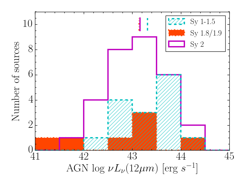
Figure 2: Derived AGN rest-frame 12 $\mu$m luminosities distribution for Seyfert 1-1.5 galaxies (hatched cyan histogram), Seyfert 1.8/1.9 galaxies (filled orange histogram) and Seyfert 2 galaxies (magenta histogram). The vertical lines indicate the median of the distributions.

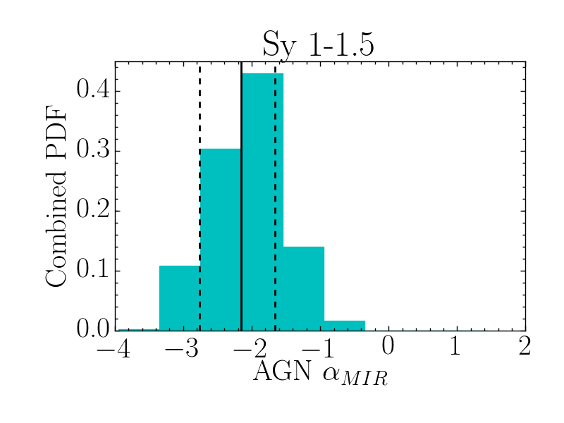
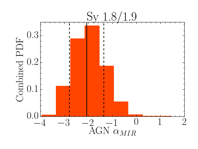
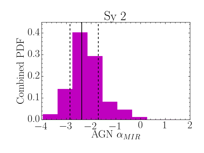
Figure 3: Combined probability distribution functions of the AGN MIR ($8.1-12.5$ $\mu$m) spectral index derived with deblendIRS. In all panels the solid lines indicate the median of the distributions and the dashed lines the 16% and 84% percentiles. The panels are for the Seyfert 1-1.5 galaxies (cyan, left), Seyfert 1.8/1.9 galaxies (orange, middle), and Seyfert 2 galaxies (magenta, right).

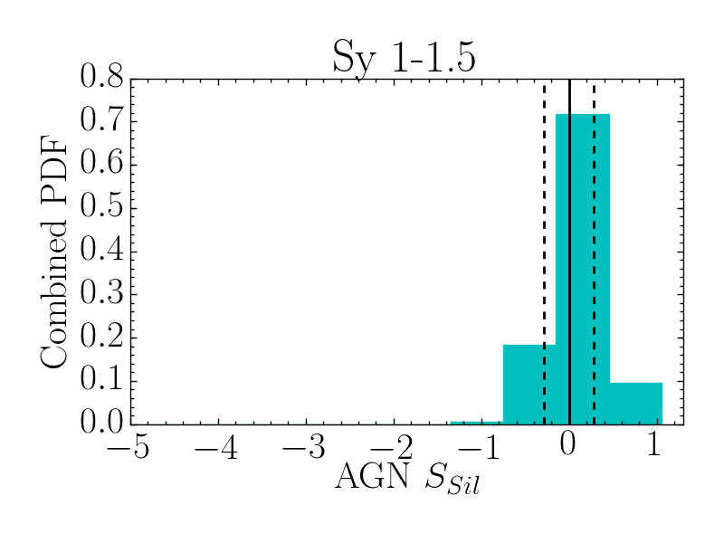
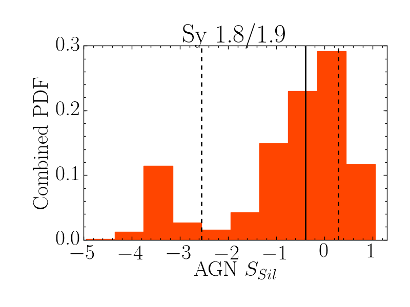
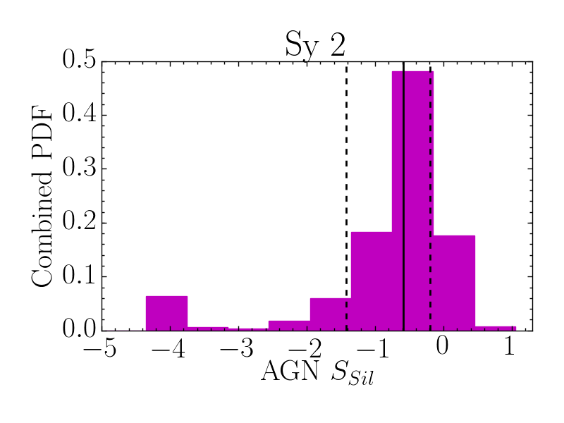
Figure 4: Combined probability distribution functions of the AGN strength of the silicate feature derived with deblendIRS. In all panels the solid lines indicate the median of the distributions and the dashed lines the 16% and 84% percentiles. The panels are for the Seyfert 1-1.5 galaxies (cyan, left), Seyfert 1.8/1.9 galaxies (orange, middle), and Seyfert 2 galaxies (magenta, right).

Table 4: Statistics of the combined probability distributions

Type	N	AGN $\alpha_{\rm MIR}$	AGN $S_{\rm Sil}$	AGN Fraction
Seyfert 1-1.5	15	-2.2 [-2.8, -1.7]	0.0 [-0.3, 0.3]	0.82 [0.68, 0.96]
Seyfert 1.8/1.9	7	-2.1 [-2.8, -1.4]	-0.4 [-2.6, 0.3]	0.86 [0.75, 0.97]
Seyfert 2	30	-2.4 [-2.9, -1.7]	-0.6 [-1.4, -0.2]	0.90 [0.76, 0.98]
Seyfert 2 (CAT3D models)	19	-2.6 [-2.9, -2.0]	-0.4 [-0.8, -0.1]	0.88 [0.73, 0.96]

Notes.– The AGN MIR spectral index is estimated in the $8.1-12.5$ $\mu$m range. The AGN fractional contribution refers to the $5-15$ $\mu$m luminosity. We give the median value and in parenthesis the 16% and 84% percentiles.

3.2 MIR properties of AGN

The first result from the spectral decomposition is that the AGN component dominates the MIR emission (over the $5-15\,\mu$m spectral range) on nuclear scales (typically 100-150 pc), with a median value of 87% for the full sample. Moreover, the AGN contribution is similar for the Seyfert 2 and Seyfert 1-1.5 in our sample (median values of 88% and 86%, respectively). The number of Seyfert 1.8/1.9 galaxies is small for statistics, so the slightly difference in their median value (80%) is not significant. We note, however, that the physical sizes covered by the slits of the Seyfert 1-1.5 nuclei are larger than those of the Seyfert 2 nuclei, on average. This means that if the slits were covering similar physical sizes for type 1-1.5 and 2 in our sample, then the AGN fractional contribution in the MIR in Seyfert 1 nuclei should be slightly higher. This is in agreement with the prediction of a nearly isotropic emission at $12\,\mu$m of the clumpy torus models of Nenkova et al. (2008b) and the similarity of the MIR emission of type 1 and type 2 AGN when compared with their hard X-ray luminosity, which is a proxy for the AGN bolometric luminosity (see e.g., Alonso-Herrero et al., 2001; Krabbe et al., 2001; Lutz et al., 2004; Gandhi et al., 2009; Levenson et al., 2009; Asmus et al., 2015). These observational differences in the MIR between type 1 and type 2 are found only to be at most a factor of two (Burtscher et al., 2015). Accordingly, we also find from the spectral decomposition that the typical AGN luminosities at rest-frame 12 $\mu$m of Seyfert 1-1.5 galaxies (median $\log(\nu L_{12\mu{\rm m}}/{\rm erg\,s}^{-1})=43.3$) are only slightly higher than those of Seyfert 2 galaxies (median $\log(\nu L_{12\mu{\rm m}}/{\rm erg\,s}^{-1})=43.2$) in our sample (see also Fig. 2).

In terms of the strength of the AGN silicate feature, the Seyfert 2 and Seyfert 1.8/1.9 have a median value of $S_{\rm Sil}=-0.5$ and $S_{\rm Sil}=-0.3$, respectively, whereas the Seyfert 1-1.5 typically show a flat or slightly in emission feature (median $S_{\rm Sil}=0.0$) and show a narrower range of fitted values. This indicates that the behaviour of the Seyfert 1.8/1.9 is closer to the Seyfert 2 than to the Seyfert 1-1.5 in terms of the strength of the silicate feature. The difference in the strength of the silicate feature is a well known property as Seyfert 1-1.5 generally show the silicate feature in emission and the Seyfert 2 galaxies in absorption (Shi et al. 2006, Thompson et al. 2009, Alonso-Herrero et al. 2014, but also see Hatziminaoglou et al. 2015). However, the difference in the strength of the silicate feature is not necessarily reflecting the properties of the torus because the MIR nuclear emission of some Seyfert galaxies may be due to extended dust components in the host galaxy (Goulding et al., 2012) even on sub-arcsecond scales (Roche et al., 2006; Hönig et al., 2010; Alonso-Herrero et al., 2011; González-Martín et al., 2013; Alonso-Herrero et al., 2014, 2016a). We will come back to this issue when we compare the observations with the CAT3D torus model predictions in Section 4.4. The median values of the fitted AGN MIR spectral indices are $\alpha_{\rm MIR}=-2.1$, $\alpha_{\rm MIR}=-2.1$ and $\alpha_{\rm MIR}=-2.3$ for Seyfert 1-1.5, Seyfert 1.8/1.9 and Seyfert 2, respectively but the ranges are similar for all Seyfert types in our sample. The difference in the MIR spectral index has also been noted by, among many works, Ramos Almeida et al. (2011) who found that Seyfert 2 show steeper $1-18\,\mu$m spectral energy distributions (SEDs) than Seyfert 1. However, they found that the difference in the $8-13\,\mu$m spectral range was small (see also Alonso-Herrero et al., 2014).

3.3 Comparison for different Seyfert types and other AGN

To make a statistical comparison of the MIR properties of Seyfert 2 and Seyfert 1-1.5 we obtained the combined PDF of each of the subsamples as a simple average of the PDF of the individual galaxies for the AGN MIR spectral index, the strength of the silicate feature and the AGN fractional contribution within the slit to the $5-15$ $\mu$m luminosity. Figure 3 shows that the peaks of the combined PDF of the AGN MIR spectral index are similar for all the Seyfert types although the distribution is slightly narrower for the Seyfert 1-1.5 nuclei (see also the statistics in Table 4). However, the differences between different Seyfert types are more apparent for the combined PDF of the silicate strength. Not only the peaks of the combined PDFs are significantly different for the three types (as also noted for the individual fits in the previous section) but the distributions differ. The Seyfert 1.8/1.9 and Seyfert 2 nuclei peak at the feature in absorption and also show a broad tail towards deep silicate absorptions whereas the Seyfert 1-1.5 show a narrow distribution peaking at $S_{\rm Sil}=0.0$. This is clearly seen in Fig. 4.

We can compare the AGN MIR properties of our Seyfert galaxies with those of a IR-weak quasars (type 1) derived by Alonso-Herrero et al. (2016b). This sample includes 10 optically selected local quasars, mostly Palomar-Green (PG) quasars, with sub-arcsecond MIR spectroscopy and for which the AGN MIR spectral properties were derived with a similar methodology as the Seyfert galaxies (Section 3.1). These quasars are classified as IR-weak quasars based on their total IR to optical B-band luminosity ratios. We refer the reader to Alonso-Herrero et al. (2016b) for further details on the quasar sample. The combined PDFs of the IR-weak quasars (see table 6 of Alonso-Herrero et al., 2016b) have median values for the AGN MIR spectral index of $\alpha_{\rm MIR}=-1.7$ ($1\sigma$ confidence interval of [$-2.4$, $-1.0$]) and for the strength of the silicate feature of $S_{\rm Sil}=0.1$ ($1\sigma$ confidence interval of [$-0.2$, 0.3]). Therefore, the quasars have significantly flatter AGN MIR spectral indices than the Seyfert 1-1.5 ($\alpha_{\rm MIR}=-2.1$) but similar strengths of the silicate feature. In Section 4.4 we will use clumpy torus model predictions to see whether these differences also imply differences in the torus properties for the different types of AGN.

4 Statistical comparison with the CAT3D clumpy torus models

4.1 Brief description of the CAT3D models

In this work we make use of the Hönig & Kishimoto (2010) CAT3D clumpy torus models that provide the model SED for clumpy dust emission in a torus around the AGN accretion disk. These models are characterised by six parameters that have direct influence on the IR dust SEDs of AGN. These are: (1) the power-law index of the radial dust-cloud distribution $a$, that is $\propto r^{a}$; (2) the half-covering angle of the torus $\theta_{0}$; (3) the number of clouds along an equatorial line-of-sight $N_{0}$; (4) the torus outer radius $R_{\rm out}$; (5) the optical depth of the individual clouds $\tau_{\rm V}$; and (6) the inclination ( i.e., the viewing angle) $i$. In Fig. 5 we show a sketch of some of the CAT3D torus model parameters. The AGN is assumed to be radiating in an isotropic manner. However, in Section 4.6 we will investigate very briefly the effects of introducing anisotropic AGN radiation on the predicted MIR properties of the clumpy torus models.

Table 5: Parameters of the CAT3D clumpy torus models.

Parameter	Symbol	Old models	New models
Index cloud radial distribution	$a$	[0.00, -2.00] steps of 0.5	[0.50, -1.75] steps of 0.25
Torus half-covering angle	$\theta_{0}$	30°, 45°, 60°, 85°	30°, 45°, 60°
Clouds along equatorial direction	$N_{0}$	2.5, 5.0, 7.5, 10.0	2.5, 5.0, 7.5, (10.0, 12.5)∗
Cloud optical depth	$\tau_{\rm V}$	30, 50, 80	50
Torus outer radius	$R_{\rm out}$	150	450
Inclination	$i$	[0°, 90°] steps of 15°	[0°, 90°] steps of 15°

Notes— The outer radius is measured in units of the sublimation radius. ^∗The values of $N_{0}=10,\,12.5$ are only for models with $a\leq 0$ for computational reasons.

To calculate the IR SEDs of these models several steps are carried out. The first step is to simulate each cloud by Monte Carlo radiative transfer simulations. Then, dust clouds are randomly distributed around the AGN, according to the physical and geometrical parameters, each one associated with a model cloud from the first step. The final torus SED is calculated via raytracing along the line-of-sight from each cloud to the observer. This method allows to take into account the three dimensional distribution of clouds and the statistical variations of randomly distributed clouds. We refer the reader to Hönig & Kishimoto (2010) for a complete description of the calculations.

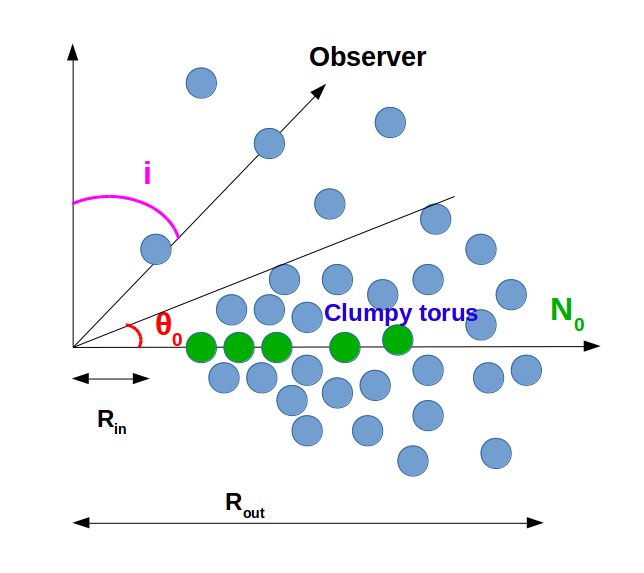
Figure 5: Representation of the CAT3D clumpy torus showing some of the parameters that characterise the models, namely the half-covering angle $\theta_{0}$, in red; the inclination $i$, in magenta, the number of clouds along an equatorial line-of-sight $N_{0}$, in green; and the inner and outer torus radii $R_{\rm in}$ and $R_{\rm out}$ respectively, in black.

4.2 New CAT3D runs with a physical dust sublimation model

The CAT3D clumpy torus models published by Hönig & Kishimoto (2010) (hereafter old models) assumed a standard ISM composition for the dust, containing 47% of graphite and 53% of silicates. In this work we present a new version of the models (hereafter referred to as new models) that includes additional more realistic physics in an attempt to model the differential dust grain sublimation. Graphite grains can sustain higher temperatures than silicate grains, with the former being able to heat up to $\sim$ $1900-2000$ K and the latter sublimating at $\sim$ $800-1200$ K, depending on density (Phinney, 1989).

The new sublimation model assumes that silicates are sublimated away once their temperature goes above 1250 K. This means that all those clouds at distances from the AGN as to heat up to temperatures above 1250 K will not contain any silicates. Therefore, in the new models the absorption and scattering efficiencies are adjusted accordingly. In addition, the hottest dust at $T\simeq 1900\,$K will only contain larger graphite grains, that is, the minimum grain size for the ISM dust size distribution is increased from 0.025 $\mu$m to 0.075 $\mu$m. This accounts for the fact that small grains are cooling less efficiently and will reach the sublimation temperature at larger distances than larger grains. As we shall see, since graphites have higher emissivity, this will result in bluer NIR to MIR SEDs for a given set of torus model parameters than in the old models, which had a standard ISM dust composition without a sublimation model. We note that the different sublimation temperatures included in the new models are unique to these models and are not taken into account in other available clumpy torus models (e.g., Schartmann et al., 2008; Nenkova et al., 2008a, b), although smooth torus models have used various approaches to differential sublimation (e.g., Granato & Danese, 1994; Schartmann et al., 2005; Fritz et al., 2006).

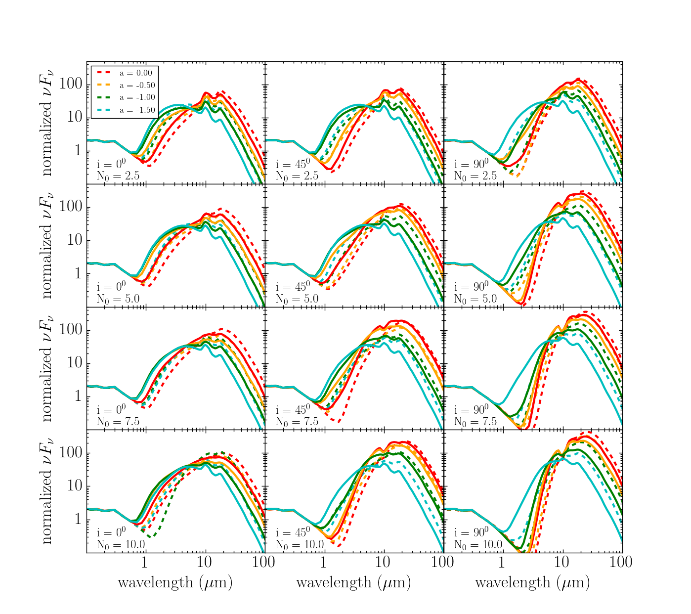
Figure 6: Examples of the CAT3D clumpy torus SEDs for the old models (dashed lines) and new models (solid lines) normalised at 0.5 $\mu$m. From top to bottom, the rows show an increasing number of clouds along an equatorial line-of-sight, $N_{0}=$2.5, 5.0, 7.5, and 10.0, respectively. The left column shows models for an inclination of 0°, the middle column is for $i=45$° and the right column is for $i=90$°. In each panel we show the SEDs for one random cloud distribution for $a=0.00$ (red), $a=-0.50$ (orange), $a=-1.00$ (green), and $a=-1.50$ (cyan). They all have fixed values of $\tau_{\rm V}=50$ and $\theta_{0}=45$°.

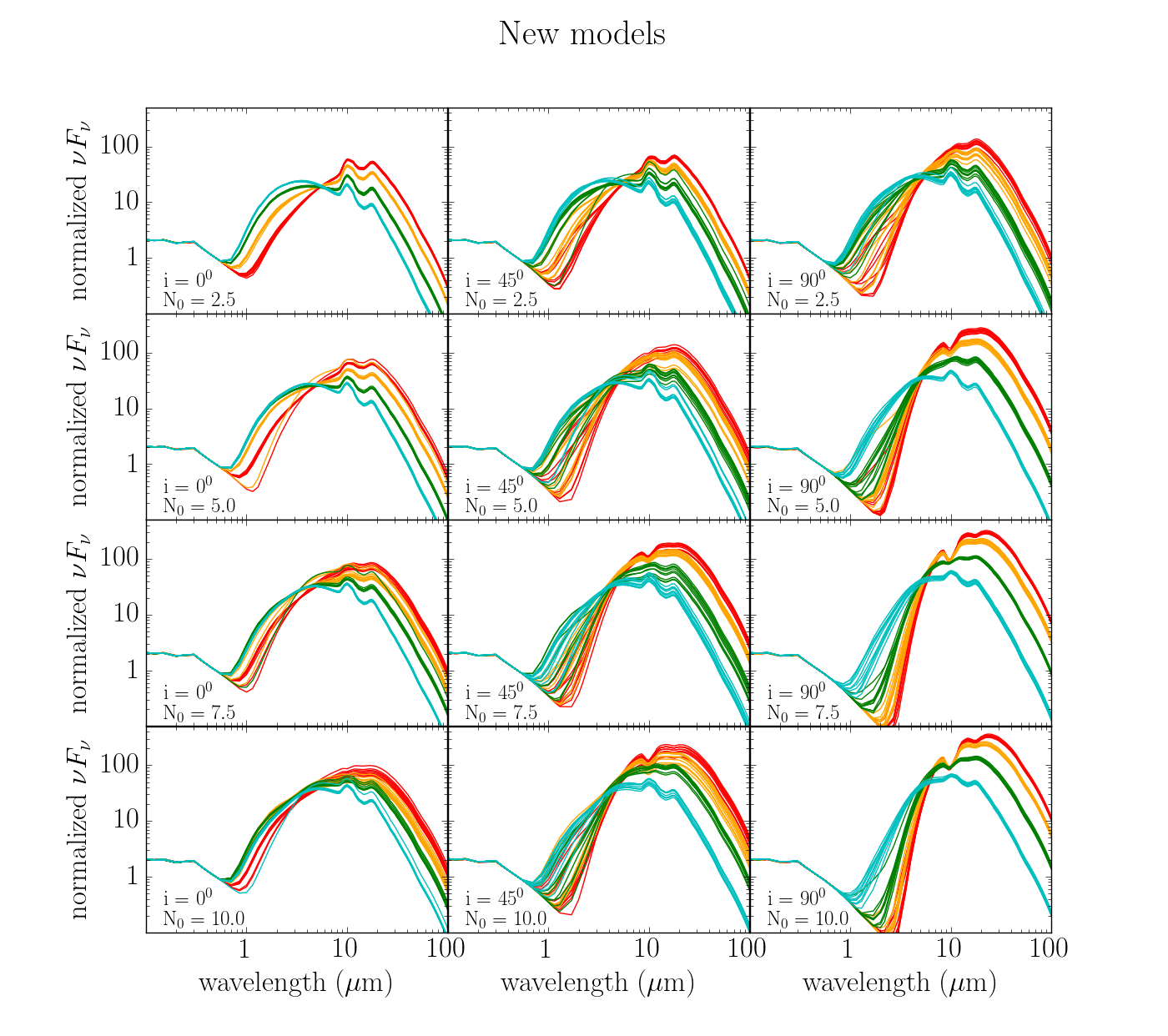
Figure 7: Same as Fig. 6 but only for the new models and showing ten random distributions of clouds for each configuration of parameters.

The old and the new models cover different ranges of the torus parameters. In Table 5 we summarize the parameter values and ranges used in the old and new models. The index of the radial distribution of clouds $a$ covers different ranges, namely [0.00, -2.00] for the old models and [0.50, -1.75] for the new ones, and different steps of 0.50 and 0.25, respectively. We note that for the new models we are adding inverted radial cloud distributions (positive values of $a$). Although, probably not very common, inverted radial distributions resemble a disk-like accretion flow that thins out towards the inner radius. This may be the kind of geometry needed to explain the population of hot dust poor quasars (Hao et al., 2010). In the case of the half-covering angle of the torus $\theta_{0}$, the old models provided more values ($\theta_{0}=$30°, 45°, 60°, 85°) than the new ones ($\theta_{0}=$30°, 45°, 60°). For the number of clouds $N_{0}$ the ranges are also different, [2.5, 10.0] for the old models and [2.5, 12.5] for the new models, both in steps of 2.5.

The new and old CAT3D models have different values of the torus outer radius $R_{\rm out}$ (measured in units of the sublimation radius, see Table 5) due to the smaller dust sublimation radius of the graphite/large dust grains than the silicate grains. The grain sublimation radius is proportional to the square root of the AGN luminosity. For $L_{\rm AGN}=10^{46}\,{\rm erg\,s}^{-1}$, the sublimation radius is 0.5 pc for large grains and 0.955 pc for the typical ISM dust composition (see table 2 of Hönig & Kishimoto, 2010). Also, the value of the outer radius of the torus needs to be sufficiently large so that it encompasses the physical sizes of the torus measured at all wavelengths and was chosen to have the same size range as with the old models. In the old models we have three values of cloud optical depth $\tau_{\rm V}$, 30, 50, and 80, whereas the new models only have one value $\tau_{\rm V}$=50. The range of the inclination $i$ is the same for both the old and the new models, from 0° to 90° in steps of 15°.

As explained above, the old and new models cover different ranges of torus parameters. We have a total of 1680 parameter configurations for old models and 966 configurations for new models, with 336 configurations sharing the same values of the torus model parameters. For each configuration of parameters, we have one SED obtained from a random arrangement of clouds for the old models and ten for the new ones, obtained from ten random distributions of the clouds satisfying the same configuration of parameters.

In Fig. 6 we show some examples of SEDs (in units of $\nu f_{\nu}$) for the old and the new models in dashed and solid lines respectively, for a random cloud distribution. Each column represents a different inclination ($i=0$°, 45°, and 90°) and each row different values of the number of clouds in the equatorial line-of-sight ($N_{0}$ = 2.5, 5.0, 7.5, and 10.0). They all have fixed values of $\tau_{\rm V}=50$ and $\theta_{0}=45$°. Each panel shows four different values of the power-law index of the radial dust-cloud distribution, $a$, indicated with different colours. For both the old and new models the total SEDs becomes redder for flatter radial cloud distributions (more positive values of $a$). As explained in Hönig & Kishimoto (2010), this is because flat power-law radial distributions have more cool dust at larger radial distances. There are differences in the continuum shape depending of the value of $a$. For the flat and nearly flat distributions ($a=0.0$ and $a=-0.50$), the continuum peaks at longer wavelengths than for the steeper distributions ($a=-1.0$ and $a=-1.50$). This is because in the steeper distributions there is more dust at small radial distances from the AGN so the average dust temperature is higher (Hönig & Kishimoto, 2010). This trend does not depend on the inclination.

The $a$ values also have an effect in the strength of the silicate feature. For the torus parameters represented in Fig. 6 with the steepest radial distribution of clouds ($a=-1.5$), the silicate feature is always in emission, whereas for the rest of the $a$ values the strength of the feature depends on the values of $N_{0}$ and the inclination. While the SEDs have a substantial dependence on $a$, the dependence on $N_{0}$ is small. This dependence on $N_{0}$ is more important for the strength of the silicate feature than for the shape of the SED (which is also related to $\alpha_{\rm MIR}$, see next section). The silicate feature in emission is the strongest for $N_{0}$ = 2.5, whereas the feature becomes less prominent when there are more clouds along the equatorial direction (larger values of $N_{0}$). In the cases of the silicate in absorption, more clouds $N_{0}$ and higher inclinations result in deeper absorptions. This is because changing $N_{0}$ has the effect that the inner and hotter part of the dust distribution becomes more obscured and more blocked along any light-of-sight. As a result, the effectively visible clouds are further away from the AGN and, thus, cooler. These cooler clouds are more likely to show silicate absorption in their source functions. This effect, which is a particularity of a clumpy distribution, is combined with the fact that the self-obscuration/extinction within the dust distribution reduces silicate emission features or turns them into absorption features. As expected, the new models have bluer NIR to MIR SEDs for a given set of torus parameters than the old models. The differences in the shape are more noticeable for the steepest radial cloud distributions ($a=-1.5$), as there is more dust at small distances from the AGN, containing only graphite for the new models while the old models have silicates and graphites at the same distance. The differences also increase when there are more clouds along the equatorial direction (larger values of $N_{0}$) and for more inclined views.

In Fig. 7 we show the SEDs for the new models, as in Fig. 6, but representing the ten random realisations of clouds computed for each configuration of torus model parameters. The differences between the random distributions for the same parameters are more apparent for more inclined views and for the flattest radial distributions of the torus clouds ($a=0.0$ and $a=-0.50$). This figure shows the importance of doing several random realisations instead of using only one. This is further discussed in Section 4.3.

4.3 CAT3D predictions for the MIR emission

In this section we present the CAT3D torus model predictions for the MIR emission of AGN and in particular for the properties we analysed in Section 3.2, namely the MIR spectral index and the strength of the silicate feature. As explained by Hönig & Kishimoto (2010), although the angular size of the torus, $\theta_{0}$, could be an additional source of degeneracy, there is a strong relation between the index of the dust radial distribution, $a$ and the MIR spectral index. There is also a strong relation between the number of clouds along the equatorial direction, $N_{0}$, and the strength of the silicate feature, even though the strength of the silicate feature also depends on $a$ and $\tau_{\rm V}$. Using the clumpy torus models of Nenkova et al. (2008a, b), Ramos Almeida et al. (2014) investigated the sensitivity of different observations in the near and MIR to these torus model parameters. Specifically, they found that a detailed modelling of the $8-13$ $\mu$m spectroscopy (not only the spectral index and strength of the silicate feature) of Seyfert galaxies can constrain reliably the number of clouds and their optical depth.

We measured for each model SED the MIR spectral index using 8.1 and 12.5 $\mu$m as anchor points and 8 and 14 $\mu$m to fit the continuum and 10 $\mu$m for the peak of the silicates, as the CAT3D models have both, the emission and the absorption features centred at 10 $\mu$m (Hönig et al., 2010). For the old models, for each of the 1680 configurations we obtained one value of the spectral index and the strength of the silicate feature. For the new models we measured ten values for each of the 966 configurations, which allows us to estimate the average and the standard deviation for the ten values of the spectral index and the strength of the silicate feature for each configuration of parameters. The typical scatters in the measured $\alpha_{\rm MIR}$ are $0.02-0.06$, although in the case of a radial distribution index $a=0.5$ the scatter can be as high as 0.2. The typical scatter in the measured $S_{\rm Sil}$ is $0.01-0.04$. These scatters are lower than the $1\sigma$ uncertainties (16% and 84% percentiles) obtained with deblendIRS for the AGN MIR spectral index and the strength of the silicate feature distributions for the Seyfert galaxy sample (see Table 3).

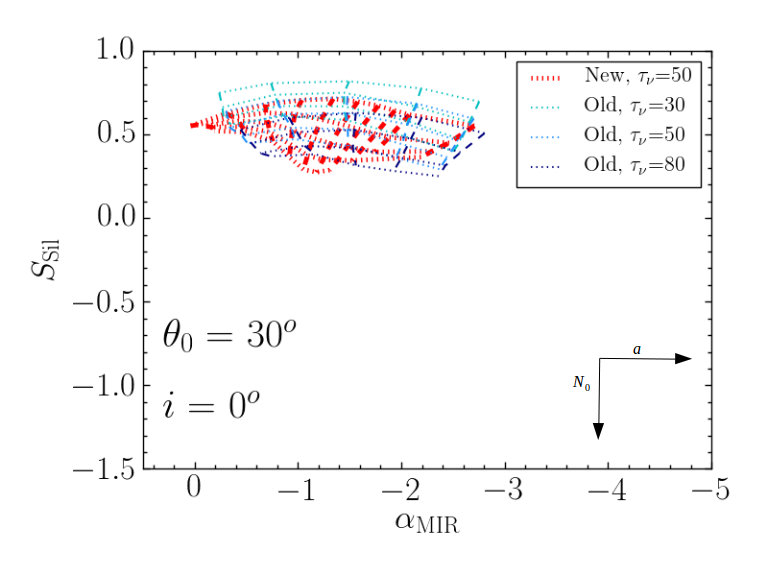
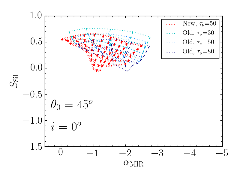
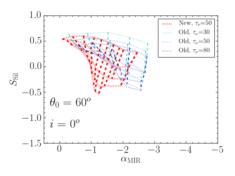
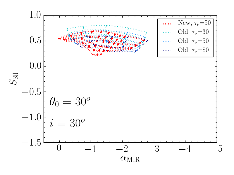
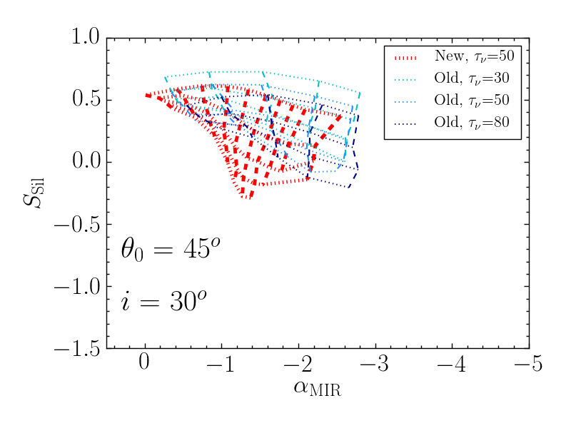
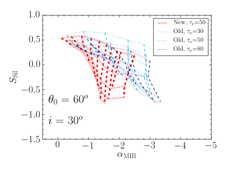
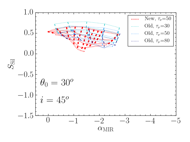
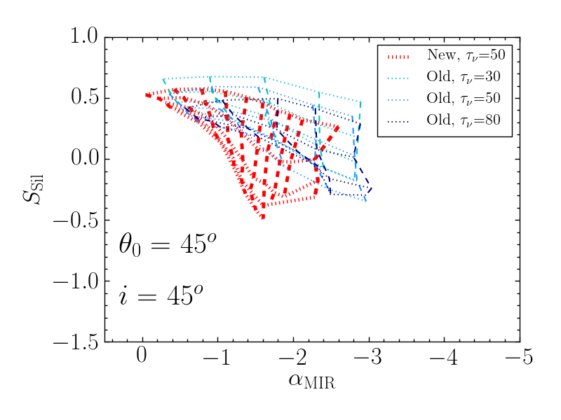
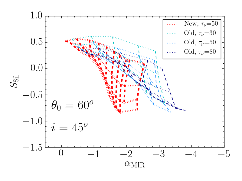
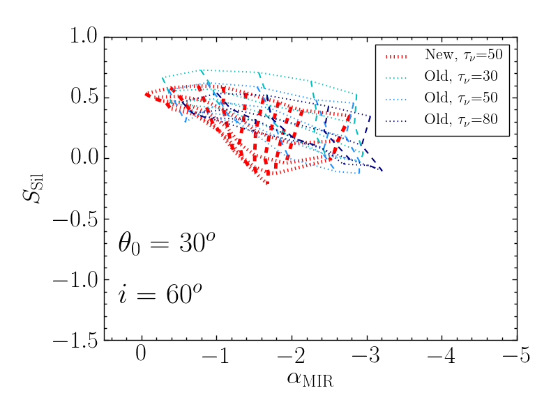
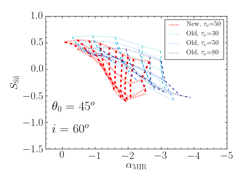
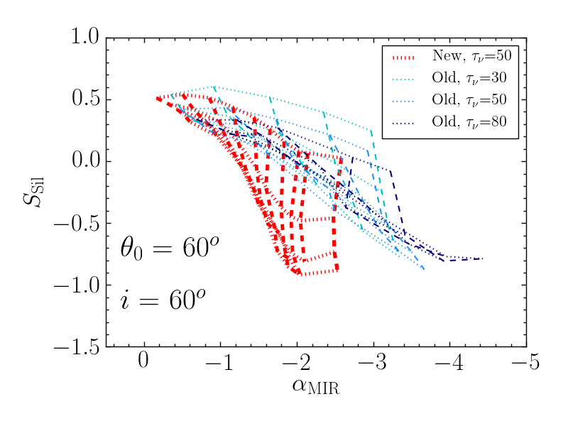
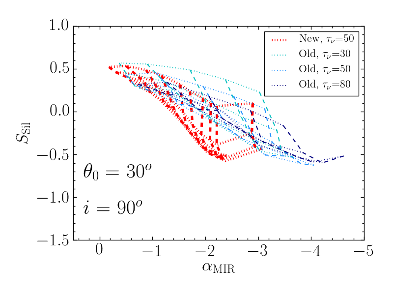
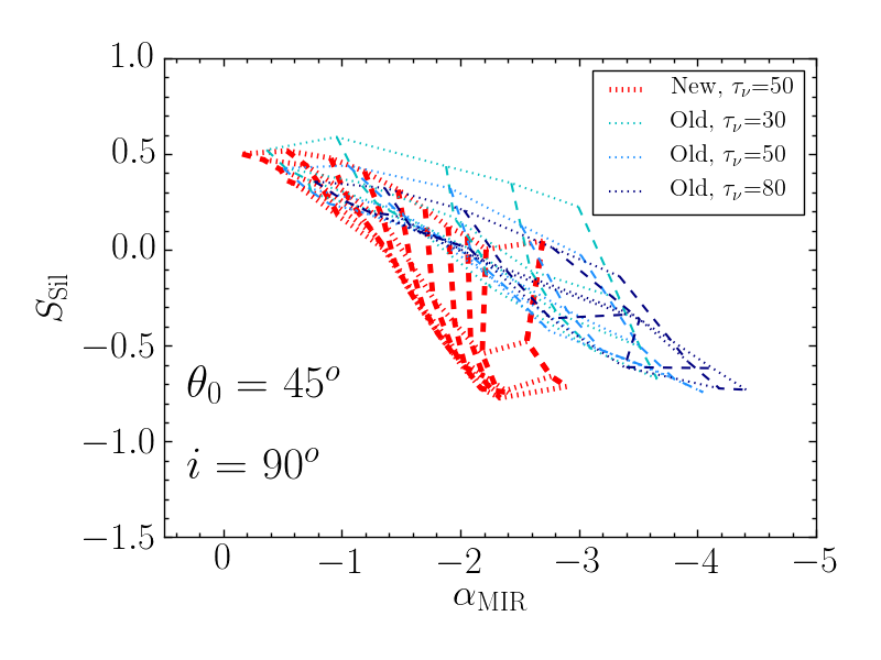
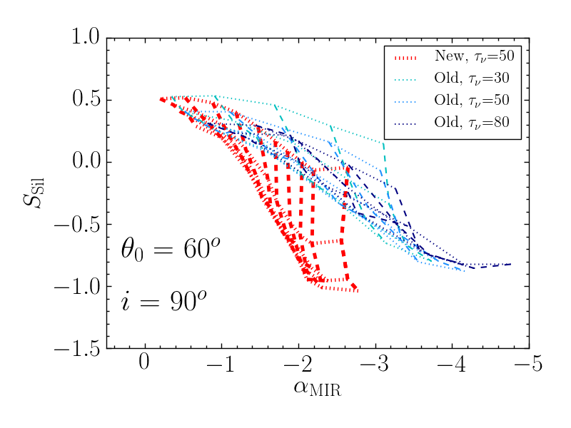
Figure 8: Strength of the silicate feature against the MIR spectral index for the CAT3D old models (in light blue $\tau_{\rm V}=30$, medium blue $\tau_{\rm V}=50$, and dark blue $\tau_{\rm V}=80$), and the CAT3D new models (in red, $\tau_{\rm V}=50$). Each panel shows the estimated values the full range of $a$ (dashed lines, values of $a$ becoming more negative to the left) and $N_{0}$ (dashed lines, larger values moving down) for a fixed inclination and torus half-covering angle. Results are shown for five viewing angles $i=0$°, 30°, 45°, 60°, and 90°.

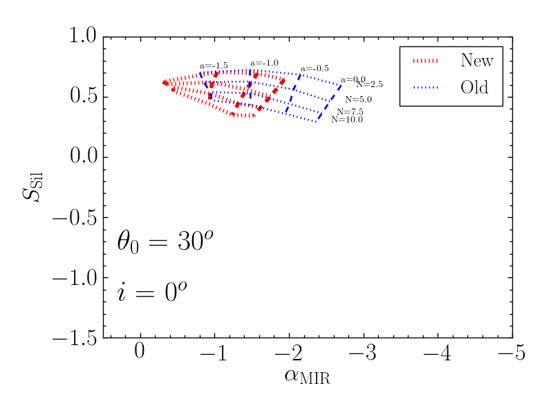
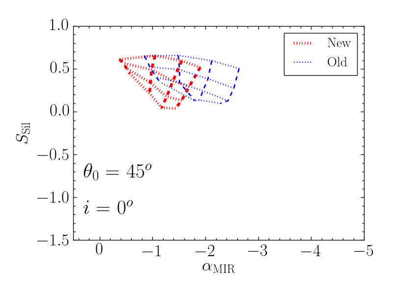
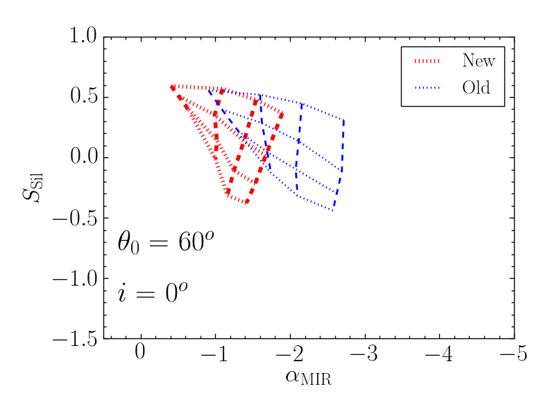
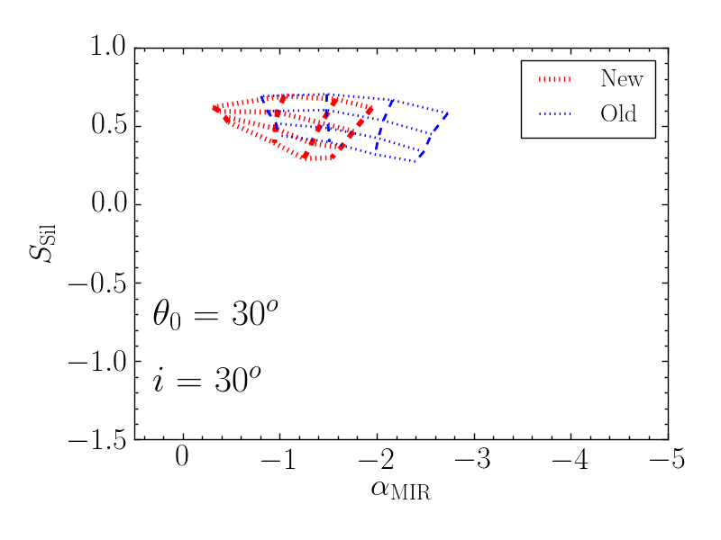
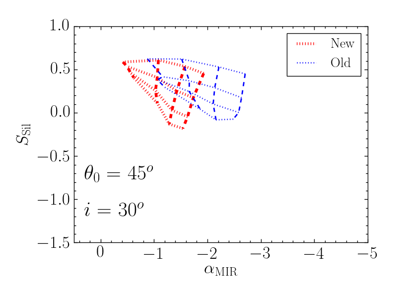
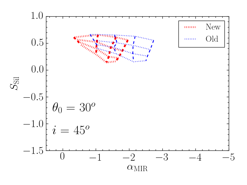
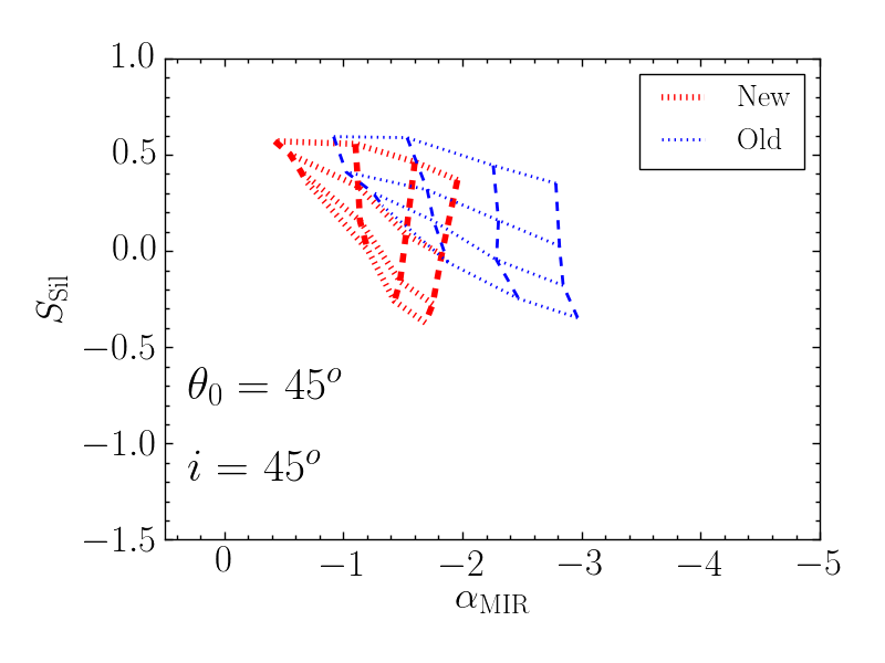
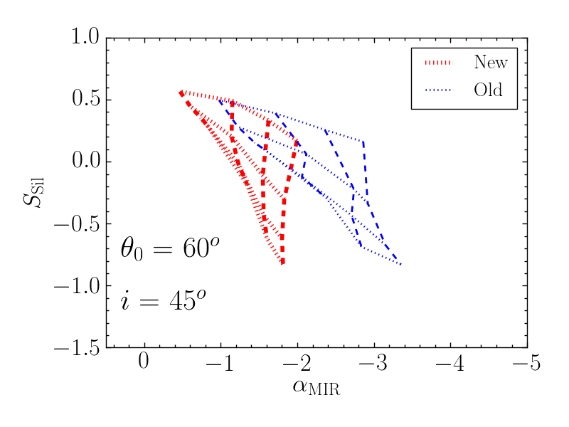
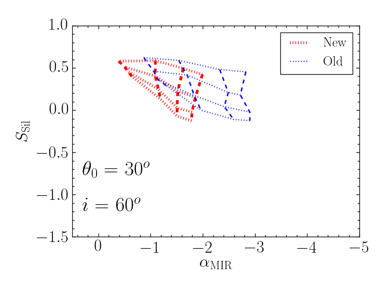
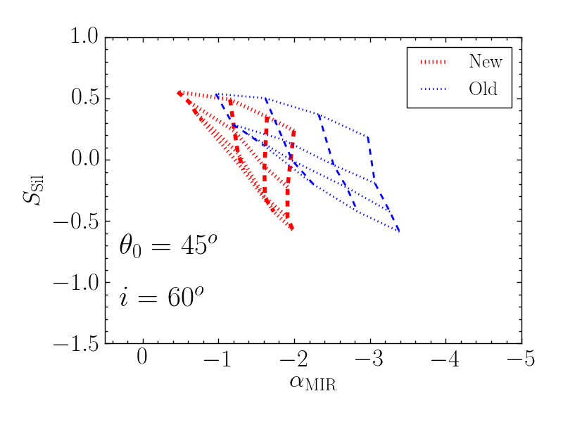
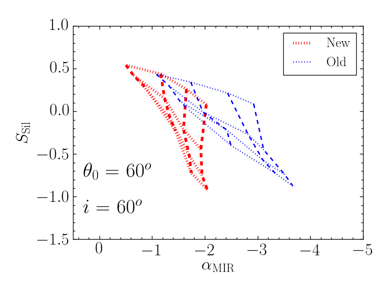
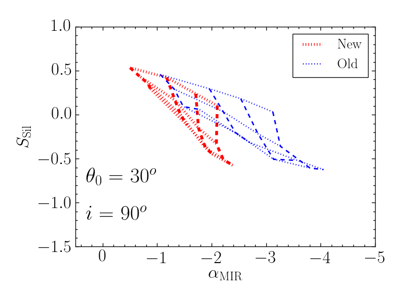
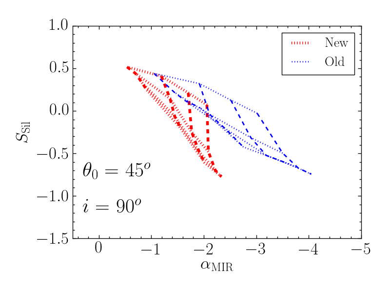
Figure 9: Comparison of the strength of the silicate feature and the MIR spectral index for the CAT3D old models (in blue), and the CAT3D new models (in red) only for the common parameters (see Table 5). Each panel shows the estimated values for different values (see top left panel) of $a$ (dotted lines) and $N_{0}$ (dashed lines) for a fixed inclination and torus half-covering angle. Results shown for five viewing angles, $i=0$°, 30°, 45°, 60°, and 90°.

In Fig. 8 we show the calculated MIR spectral index against the strength of the silicate feature for the old and new models. Each panel displays the values for the entire range in $a$ (dotted lines) and $N_{0}$ (dashed lines) for a fixed inclination and torus half-covering angle, $\theta_{0}$. We only show results for five viewing angles ($i=0$°, 30°, 45°, 60°, and 90°), one for each of the rows. As can be seen from these figures, for a given configuration of set $\theta_{0}$ and $i$, fewer clouds along the equatorial direction tend to produce weaker silicate features than configurations with more clouds with a slight dependence with the optical depth of the clouds $\tau_{\rm V}$. As explained in the previous section, increasing $N_{0}$ results in deeper silicate absorption features and reduced silicate emission features (see Section 4.2). Interestingly, for both the old and the new models for thin tori, $\theta_{0}$=30°, and values of the inclination of $i\leq 45$°, the silicate feature is always produced in emission. We can also see from these figures that thicker tori tend to decrease the strength of the silicate feature when seen in emission (that is, make it flatter) or make it deeper when the silicate is in absorption.

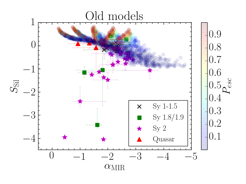
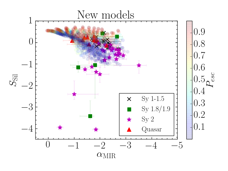
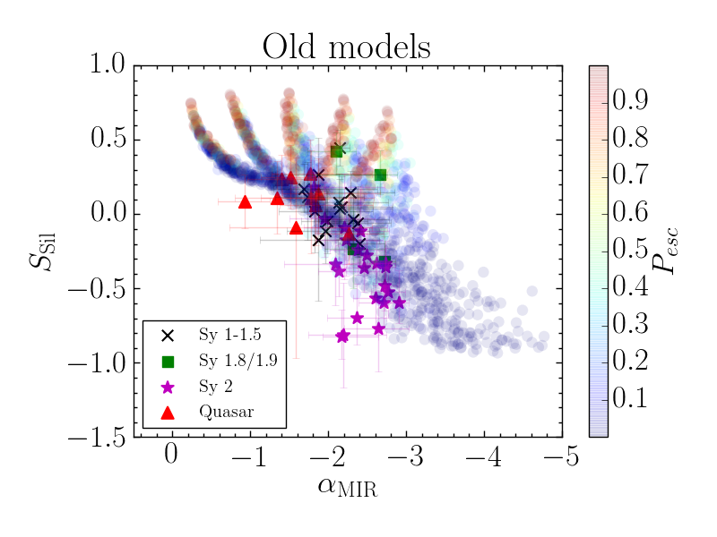
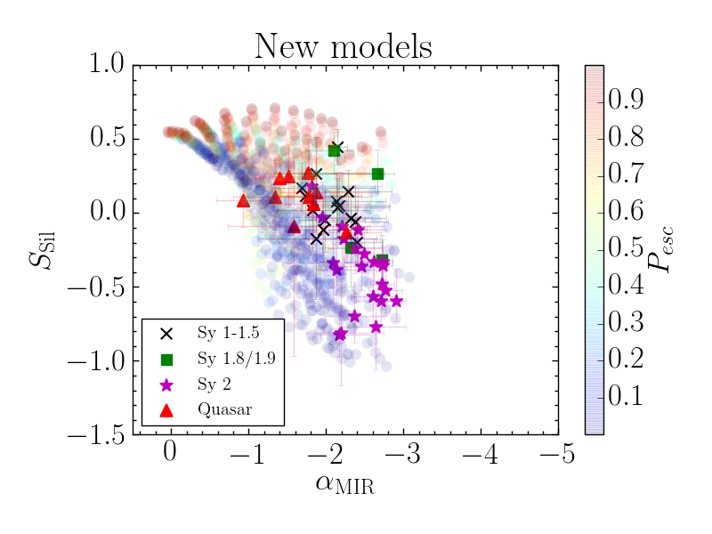
Figure 10: Top panels: MIR spectral index vs. the strength of the silicate the values for all parameters (see Table 5) of the CAT3D old torus models (left) and the new torus models (right). The model symbols (semi-transparent dots) are colour coded in terms of $P_{\rm esc}$ (see equation 1). The different types of Seyfert are shown as black crosses for the Seyfert 1-1.5 nuclei, green squares for the Seyfert 1.8/1.9, magenta stars for the Seyfert 2 nuclei, and red triangles for the IR-weak quasars (Alonso-Herrero et al., 2016b). Bottom: Same as upper panels but excluding those galaxies not represented by the CAT3D models and thus zooming in the Y axis for $S_{\rm Sil}>-1.5$.

For the predicted MIR ($8.1-12.5$ $\mu$m) spectral index there is a dependence with the index of the radial cloud distribution $a$ and the half-covering angle of the torus $\theta_{0}$ in the sense that thicker tori and flatter dust radial cloud distributions (less negative values of the index of the radial distribution of the clouds $a$) produce more negative MIR spectral indices (redder SEDs). This is because the flat and nearly flat distributions ($a=0.0$ and $a=-0.5$) have more cold dust at larger radial distances whereas for the steeper dust radial cloud distributions most of the dust is at small radial distances from the AGN, so the average dust temperature is higher and have relatively more emission at shorter wavelengths. In the case of the half-covering angle of the torus $\theta_{0}$, the effect is due to the self-obscuration within the dust distribution, i.e. for thicker tori we are shielding more hotter clouds, making the overall SED redder. However, this strictly applies only to geometries and viewing angles were self-obscuration is not strong (that is, few clouds and low-intermediate values of $i$. On the other hand, $\alpha_{\rm MIR}$ for a given configuration of $\theta_{0}$, range of values of $a$ and $\tau_{\rm V}$ has only a slight dependence on the viewing angle (i.e., compare models in the vertical panels of Fig. 8) with the spectral index becoming steeper for more inclined views.

Hönig & Kishimoto (2010) stated that there is very little dependence of model output SED on the assumed optical depth of the clouds and that $\tau_{\rm V}=50$ for a standard ISM composition gives a good representation of observations. In Fig. 8 we can see indeed that the dependence of the MIR spectra l index and strength of the silicate feature on $\tau_{\rm V}$ is small for the old models. The only noticeable trend when the silicate feature is in emission is that the $\tau_{\rm V}=30$ models always produce a stronger feature than the $\tau_{\rm V}=80$ models. For inclinations $i>$45°  when the feature is observed in absorption also the $\tau_{\rm V}=30$ models always produce a stronger feature than the $\tau_{\rm V}=80$ models. This is due to a change in the MIR for the optical depth. This leads to source functions preferentially with deeper features and also produces deeper features from self-absorption/extinction by other clouds.

In order to make a better comparison between the old and the new models we repeat in Fig. 9 the comparison of the strength of the silicate feature and the MIR spectral index for the old and new models but only for the parameters in common. That is, $\tau_{\rm V}=$ 50; $a=0.00$, -0.50, -1.00, -1.50; and $N_{0}$ = 2.5, 5.0, 7.5, 10.0. As for Fig. 8, we only show five inclinations. The most noticeable difference between the models is that for the same configuration (same $i$, $\theta_{0}$, $a$ and $N_{0}$) the old models reach a more negative value of the MIR spectral index. This is expected due to the dust sublimation model introduced in the new models (Section 4.2). Due to self-obscuration effects becoming important further in, the silicate-bearing clouds are on average cooler, thereby contributing more to silicate absorption via obscuration/extinction than to emission. For this reason, it is necessary to include positive values of $a$ (that is, inverted radial distribution of clouds) for the new models, in order to reach more negative values of $\alpha_{\rm MIR}$. In the case of the strength of the silicate feature, the new models appear to produce always slightly deeper silicate features with the differences becoming larger for the thickest tori and more inclined views. For relatively inclined cases, this effect is due to the differential dust sublimation. The strongest emission features are always produced by the hottest silicate dust. While for the old models the hottest silicate temperature is 1500 K, for the new models it is 1250 K. So the new models are starting out with a weaker silicate feature in emission. When raytraced through the dust distribution, these get turned into absorption by self-obscuration/extinction. Since the new models started out with weaker features in emission they end up with deeper absorption features.

4.4 Comparison between old and new model predictions and observations

In this section we compare the predictions for the MIR emission of the old and new CAT3D models with our observations of Seyfert galaxies and IR-weak quasars to see if the improved physical model for the dust sublimation produces a better description of the observations. As the classification in Seyfert 1 or 2 is a probabilistic effect in torus models where the dust is distributed in clumps, to compare the models with the observations, we calculate for each model the probability that an AGN produced photon escapes unabsorbed using the following expression:

$$P_{\rm esc}=\exp\left(-N_{0}\times exp\left(\frac{-(90-i)^{2}}{{\theta_{0}}^{2}}\right)\right)$$ (1)

If the escape probability is high the models correspond statistically to a Seyfert 1 galaxy, and if the probability is low to a Seyfert 2 galaxy (Elitzur, 2012). The idea is to have a gradual transition between types instead of using an arbitrary value of the probability to separate the models between type 1 and type 2. We note that Hönig et al. (2010) used an inclination criterion to separate Seyfert 1 (inclination of $i=30$°) and Seyfert 2 (inclination of $i=75$°) models. However, Ramos Almeida et al. (2011) and Alonso-Herrero et al. (2011) used the clumpy torus models of Nenkova et al. (2008a, b) and a Bayesian approach to fit the IR SEDs of nearby Seyfert galaxies. Both works demonstrated that the viewing angle is not the only determinant torus parameter to separate out Seyfert 1 and Seyfert 2, and therefore the escape probability of an AGN-produced photon is a better way to separate the Seyfert 1 models from the Seyfert 2 models (see also Elitzur, 2012).

Fig. 10 compares the CAT3D model predictions and the observations of the Seyferts and quasars. Neither the new nor the old models explain those galaxies with nuclear deep silicate absorptions, i.e., values of the strength of the silicate feature approximately $S_{\rm Sil}<-1$. This is similar to findings by other works (Levenson et al., 2007; Sirocky et al., 2008; Alonso-Herrero et al., 2011; González-Martín et al., 2013) using the clumpy torus models of Nenkova et al. (2008a, b). There are 11 galaxies in our sample whose values are not represented by the new models and we study the possibility that they are objects with host obscuration. Eight of them are classified as Seyfert 2 and 3 of them Seyfert 1.8/1.9 galaxies. In Fig. 11 we show the distribution of the inclination of the host galaxy ($b/a$) for all galaxies and the galaxies that are not represented by the new models. We can see that the galaxies not represented by the CAT3D torus models tend to be in more edge-on galaxies (lower values of $b/a$) when compared with the entire sample. Other galaxies are in interacting systems or systems with disturbed morphologies (i.e., IC 4518W and NGC 7479).

A general result from Fig. 10 is that the new CAT3D models represent better the distributions of the MIR spectral indices and strengths of the silicate features of the IR-weak quasars, the Seyfert 2 and Seyfert 1.8/1.9 galaxies than the old ones. The Seyfert 1-1.5 are well represented with both the old and the new models. It is also noteworthy that the old models for certain parameter configurations produce very steep MIR spectra indices (up to $\alpha_{\rm MIR}=-4$) for low escape probabilities that are not observed in Seyfert nuclei or local type 1 quasars. We therefore conclude that the new models with the improved dust physics reproduce better the MIR properties of the local type 1 (IR-weak) quasars and Seyfert galaxies.

In Fig. 10 the model predictions are colour coded according to $P_{\rm esc}$. The new CAT3D models have increased $P_{\rm esc}$ at the location of the type 1 AGN (Seyferts and quasars) whereas the old models had some difficulties producing relatively red MIR colours unless there were a lot of clouds (see next section) which makes $P_{\rm esc}$ low. As expected, in this figure most Seyfert 2 nuclei are close to models with low escape probabilities, although the Seyfert 1-1.5 nuclei in this diagram are in a region populated by models with both low and relatively high escape probabilities (see next section too). However, for the new CAT3D models the majority of silicate features in emission are observed for parameter configurations resulting in relatively high escape probabilities ($P_{\rm esc}>0.7$, approximately) as also found by Nikutta et al. (2009) for the CLUMPY models.

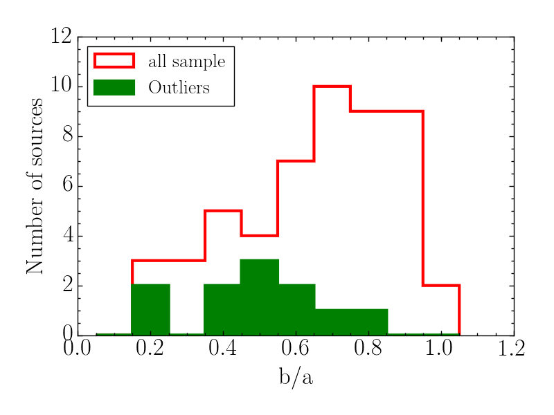
Figure 11: Distribution of the inclination of the host galaxies ($b/a$) for all the Seyfert galaxies (red histogram) and for the outliers, i.e., those Seyfert nuclei whose MIR properties are not represented by the CAT3D torus models (green filled histogram).

4.5 Constraining the CAT3D torus model parameters

In the previous sections we compared the CAT3D old and new torus models with all the Seyfert galaxies and the IR-weak quasars. In this section we focus on the old and new models and the Seyfert galaxies whose MIR properties are explained by the models. The goal is to determine if we can constrain some of the CAT3D clumpy torus model parameters from a statistical point of view. To do so, for the observations we will use the combined PDFs of the Seyfert 1-1.5, Seyfert 2 (only those reproduced by the models, see Table 4) and quasars (Alonso-Herrero et al., 2016b).

Figure 12 shows this comparison with the model symbols colour coded in terms of $P_{\rm esc}$. As noted above, the Seyfert 2 galaxies are explained by models with low photon escape probability for both the old and the new models. However, the Seyfert 1-1.5 galaxies and the quasars lie in a region of this diagram occupied by models with relatively high and low AGN photon escape probabilities. This is due to the degeneracy inherent to clumpy torus models, with models with different set of parameters producing the same values of the strength of the silicates and the MIR spectral index. On the other hand, detailed fits to the individual IR SEDs of Seyfert 1 with the clumpy torus models of Nenkova et al. (2008a, b) showed that the derived escape probabilities are never extremely high (typically $P_{\rm esc}=0.2-0.3$, see Ramos Almeida et al., 2011; Alonso-Herrero et al., 2011; Audibert et al., 2017). The escape probabilities of Seyfert 2 are generally found to be $P_{\rm esc}<0.1$. This is also in good agreement with our statistical result that the models (both the old and the new ones) with very high photon escape probabilities ($P_{\rm esc}>0.7$, approximately) tend to occupy a region of the diagram not populated by the observations (i.e., approximately $\alpha_{\rm MIR}>-1$ and $S_{\rm Sil}>0.25$).

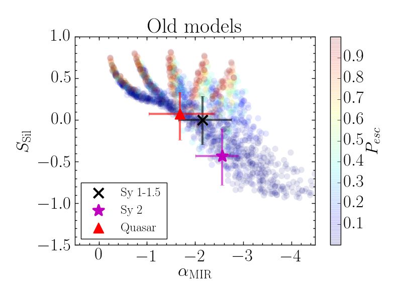
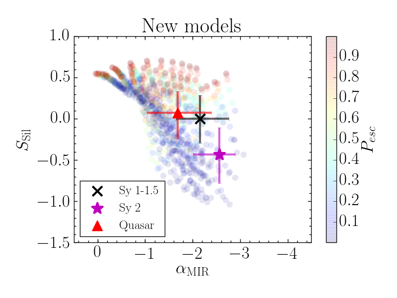
Figure 12: Same as Fig. 10 for the old and new model outputs. For the observations we plot the median values and $1\sigma$ uncertainties of the derived combined PDF of the MIR spectral index and the strength of the silicate feature as a black cross for the Seyfert 1-1.5, a magenta star symbol for those Seyfert 2 galaxies reproduced by the models (see text) and a red triangle for the IR-weak quasars from Alonso-Herrero et al. (2016b).

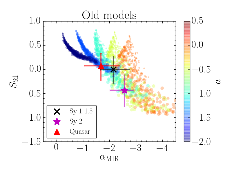
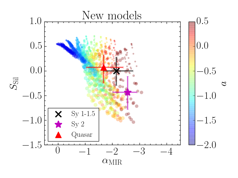
Figure 13: As Fig. 12 but the model symbols are colour coded in terms of the value the power-law index of radial dust-cloud distribution, $a$, and the size of the model symbols is proportional to the number of clouds along an equatorial line-of-sight, with the smallest symbols corresponding to $N_{0}=2.5$ and the largest symbols to $N_{0}=12.5$ (see Table 5).

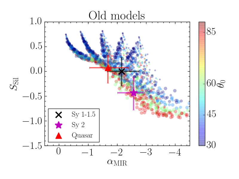
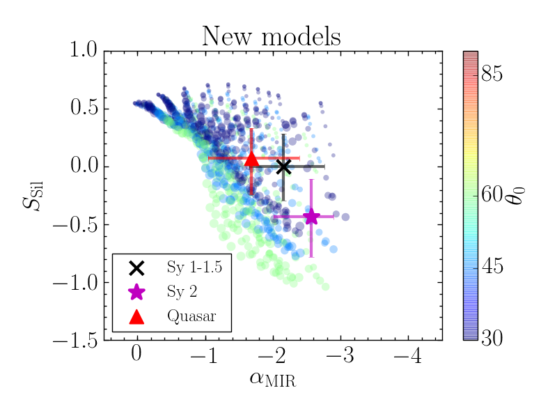
Figure 14: As Fig. 12 but the model symbols are colour coded in terms of the value the torus half-covering angle, $\theta_{0}$, and the size of the model symbols is proportional to the number of clouds along an equatorial line-of-sight, $N_{0}$ as in Fig. 13.

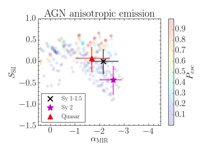
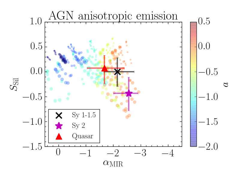
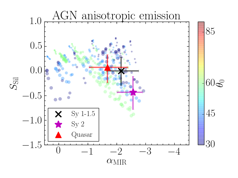
Figure 15: As the right panels of Figs. 12 (top), 13 (middle) and 14 (bottom) but showing the results for the new CAT3D models with anisotropic AGN emission.

In Fig. 13 we show the same comparison as in Fig. 12, but now we colour code the model symbols in terms of the value of the power-law index of the radial dust-cloud distribution, $a$. The size of the model symbols is proportional to the number of clouds along an equatorial line-of-sight, $N_{0}$. From a statistical point of view Seyfert 2 nuclei are reproduced with models with more clouds in the equatorial direction than type 1 AGN. For the new models, those Seyfert 1-1.5 galaxies in our sample with a nearly flat silicate feature ($S_{\rm Sil}\sim 0$) can also be reproduced with models with more clouds, whereas the Seyfert 1-1.5 galaxies with silicate emission are only reproduced with a few clouds in the equatorial direction (see also Fig. 10 where we plotted the values of the individual objects). As explained in previous sections, the increase in the number of clouds along the equatorial line-of-sight, $N_{0}$, reduces the strength of the silicate feature in emission or turns them into absorption features. This is in good agreement with the conclusions of Hönig & Kishimoto (2010), who showed that more clouds along an equatorial direction direction (larger values of $N_{0}$) produce weaker emission at 10 $\mu$m in Seyfert 1. For Seyfert 2, the silicate feature is deeper for large values of $N_{0}$. The same result was obtained by Ramos Almeida et al. (2014) with the clumpy torus models of Nenkova et al. (2008a, b). They found that for Seyfert 1, flat silicate features can also be reproduced with high values of $N_{0}$ ($\sim 10-15$) and high values of the optical depth $\tau_{V}=100-150$, whereas strong silicates in emission are produced by configurations with a few optically thin clouds along the equatorial direction. For Seyfert 2, the silicate feature in absorption is also reproduced with high $N_{0}$ ($\sim 8-15$) with $\tau_{V}\sim 50$. Ichikawa et al. (2015) also used the Nenkova et al. (2008a, b) clumpy models and found that there were statistically significant differences between the distributions of $N_{0}$ for the Seyfert 1 and the Seyfert 2 with hidden broad line region. For the old models there is more degeneracy in terms of the number of clouds for the Seyfert 1-1.5 galaxies and they can be explained with models with low and high number of clouds.

From Fig. 13 we can also set a limit on $a$ values that can reproduce our Seyfert galaxies using the CAT3D models. Very negative values of $a$, i.e., $a\leq-2.0$ for the old models and $a\leq-1.5$ for the new models, cannot reproduce the values observed in Seyfert galaxies or even the quasars. To represent the Seyfert 2 values it is necessary to have positive values of $a$ ($a=0.25,0.50$), that is, radial distributions with more clouds towards the outer parts of the torus. We also found steeper radial distributions of clouds in the old models than in the new ones. We can also conclude that there is a tendency for quasars, Seyfert 1-1.5 and Seyfert 2 to be reproduced with increasingly flatter indices of radial distributions of the torus clouds (more positive values of $a$). This is in good agreement with the result of Martínez-Paredes et al. (2017) using a detailed modelling of the nuclear SEDs with the clumpy torus models of Nenkova et al. (2008b).

We finally compare the data and the models in Fig. 14 colour coding the model symbols in terms of the torus half-covering angle, $\theta_{0}$. We can observe a tendency for the Seyfert 1-1.5 and the IR-weak quasars to be represented with relatively thinner tori ($\theta_{0}\leq 45$°) than the Seyfert 2 galaxies (old models), but there is a degeneracy produced by the clumpy torus models. This is consistent with the finding of thinner tori in Seyfert 1-1.5 than Seyfert 2 by Ramos Almeida et al. (2011) and Ichikawa et al. (2015) using fits of the IR SEDs of Seyfert nuclei. For the new models, this tendency is not observed and all galaxies are better represented with relatively thinner tori. To break this degeneracy, it is required to have information about the nuclear near-IR emission (Ramos Almeida et al., 2014).

Summarizing, we are able to constrain some of the parameter ranges of the old and new CAT3D torus models. In particular, we set a lower limit to the index of the power-law radial distribution of clouds ($a\geq-1.5$ for the old models and $a\geq-1.25$ for the new models). We derive statistical tendencies for type 1 nuclei, which are represented better with steeper dust radial distributions and thinner tori than Seyfert 2 for the old models, whereas there is more degeneracy for the new models. We also find that the MIR properties of Seyfert 2 nuclei are well reproduced with CAT3D models with a combination of parameters that result in smaller escape probabilities of AGN-produced photons.

4.6 Models with AGN anisotropic emission

We finally explore very briefly the effects on the MIR properties of introducing AGN anisotropic emission in the new CAT3D models to take into account the expected angular dependence of an AGN UV emission. We introduced a $\cos(i)$ dependence in the AGN illumination of the torus clouds as an approximation of the more general angular dependence of the UV radiation of an accretion disk $\propto 1/3\,\cos(i)*(1+2\,\cos(i))$ (see Netzer, 1987, and references therein), also adopted by other works (e.g., Hönig et al., 2006; Schartmann et al., 2005, 2008; Stalevski et al., 2012). We run models with torus parameters identical to those listed in Table 5 for the new models except for the power-law index of the radial distribution of the clouds, which is in the $a=[-2,0]$ range and in steps of 0.5. The range is the same as in the old models in order to avoid the inverted radial cloud distributions ($a$ > 0).

The anisotropy introduces a significant additional vertical temperature gradient on top of self-obscuration. For isotropic AGN emission, the projected radial temperature profile of the torus does not depend strongly on $\theta_{0}$ (or the scale height of the torus) since the temperature is approximately the same on the skin of the torus. However, in the anisotropic case, the torus surface has a lower temperature for a given distance from the AGN when the scale height is small since the incident radiation from the AGN is adjusted by $\cos(i)$. This results in redder SEDs (that is, steeper MIR spectral indices, see Fig. 15). We note however, that Stalevski et al. (2012) found no significant differences in the shape of the SEDs when including the AGN anisotropic emission in their two-phase media clumpy models. The difference in MIR predictions for CAT3D models with AGN isotropic and anisotropic emission is clearly seen in terms of the index of the radial distribution $a$. Models with indices ranging from $a=-2.0$ to $a=0$ and AGN anisotropic emission reproduce the observed range of $\alpha_{\rm MIR}$ values for Seyferts and quasars without the need for an inverted (i.e., $a>0$) radial distribution of clouds. We also note that these new models would be able to explain the rather flat MIR SEDs and shallow silicate absorptions of low luminosity AGN (González-Martín et al., 2015). However, as can also be seen from the comparison of the right panel of Fig. 13 and middle panel of Fig. 15, adding AGN anisotropic radiation alters the rather well-behaved dependence of the MIR spectral index with the index of the cloud radial distribution.

Finally, we can see that AGN anisotropy has a small effect on the strength of the silicate feature (compare e.g., right panel of Fig. 14 and bottom panel of Fig. 15, and see also Schartmann et al., 2005; Stalevski et al., 2012). Moreover, anisotropy does not suppress the $9.7\,\mu$m silicate feature in emission, as found by Manske et al. (1998) for a flared disk model with AGN anisotropic emission.

5 Summary and conclusions

The main goal of this work was to make a statistical comparison of the MIR properties of Seyfert nuclei and predictions from the CAT3D clumpy torus models of Hönig & Kishimoto (2010). We used the published version of the models (old models) with a standard ISM dust composition. We also presented new calculations including an improved physical representation of the dust sublimation properties (new models) and AGN anisotropic emission. The new CAT3D models allow graphite grains to persist at temperatures higher than the silicate dust sublimation temperature. This produces bluer NIR-to-MIR SEDs and flatter MIR spectral slopes.

We compiled ground-based MIR ($\sim 7.5-13.5\,\mu$m) spectroscopy of 52 nearby (median distance of 36 Mpc) Seyfert galaxies, using published observations taken with $8-10\,$m class telescopes with sub-arcsecond angular resolution. The sample contains fifteen Seyfert 1-1.5, seven Seyfert 1.8-1.9, and thirty Seyfert 2. They are located at a median distance of 36 Mpc and the ground-based slits cover typical nuclear regions of 101 pc in size. We decomposed the spectra using deblendIRS to disentangle the AGN MIR emission from the stellar and the PAH emission arising from the host galaxy and focused on the derived AGN MIR spectral index ($\alpha_{\rm MIR}$) and strength of the $9.7\,\mu$m silicate feature ($S_{\rm Sil}$).

The CAT3D models do not reproduce the Seyfert galaxies with deep ($S_{\rm Sil}<-1$) silicate absorption (approximately 20% of the sample), as found with other clumpy torus models. These galaxies tend to have low values of $b/a$ (highly inclined galaxies) and some of them are mergers. These are likely objects with contamination from obscuration in the host galaxy (Alonso-Herrero et al., 2011; Goulding et al., 2012; González-Martín et al., 2013). Excluding these galaxies, the new CAT3D models improve overall the representation of the quasars, Seyfert 1.8/1.9 and Seyfert 2 galaxies.

We also attempted to constrain the new CAT3D torus model parameters from a statistical point of view using the MIR observations. The Seyfert 2 galaxies are well reproduced with low photon escape probability models, as expected, whereas the type 1 AGN tend to have higher escape probabilities. The moderate silicate features in absorption of Seyfert 2 are reproduced with models with more clouds along an equatorial direction ($N_{0}$), whereas the Seyfert 1-1.5 galaxies and the IR-weak quasars with silicate emission are explained with a few clouds. There is also a tendency from quasars to Seyfert 1-1.5 to Seyfert 2 nuclei to show increasingly shallower radial cloud distributions (less negative values of $a$). This is in good agreement with previous works (Hönig & Kishimoto, 2010; Ramos Almeida et al., 2011; Ichikawa et al., 2015; Martínez-Paredes et al., 2017). Very negative values of $a$, i.e., $a\leq-2.0$ for the new models (that is, most of the clouds are concentrated towards the inner regions of the torus) tend to produce flatter MIR spectral indices and stronger silicate features than observed in Seyfert galaxies or even the quasars. In the new models most Seyfert 2 galaxies would require inverted radial cloud distributions (positive $a$). The problem with this uncommon geometry is solved by introducing a $\cos i$ dependency on the AGN illumination of the clouds (AGN anisotropic emission) which produces bluer MIR spectral indices in good agreement with the range of observed values.

In conclusion, including a more realistic dust sublimation physics as well as anisotropic AGN emission in the new CAT3D models reproduces better the overall MIR properties of local Seyfert 1-1.5, 2, and quasars. However, we cannot break fully the degeneracy in all parameters of the CAT3D models (or any other clumpy torus models) by using MIR spectroscopy alone (see also Ramos Almeida et al., 2014) even after isolating the AGN component. However, by using a large sample of Seyfert galaxies we were able uncover some differing trends between type 1-1.5 and type 2 in terms of the index of the radial distribution of the clouds $a$ and the number of clouds along the equatorial direction $N_{0}$.

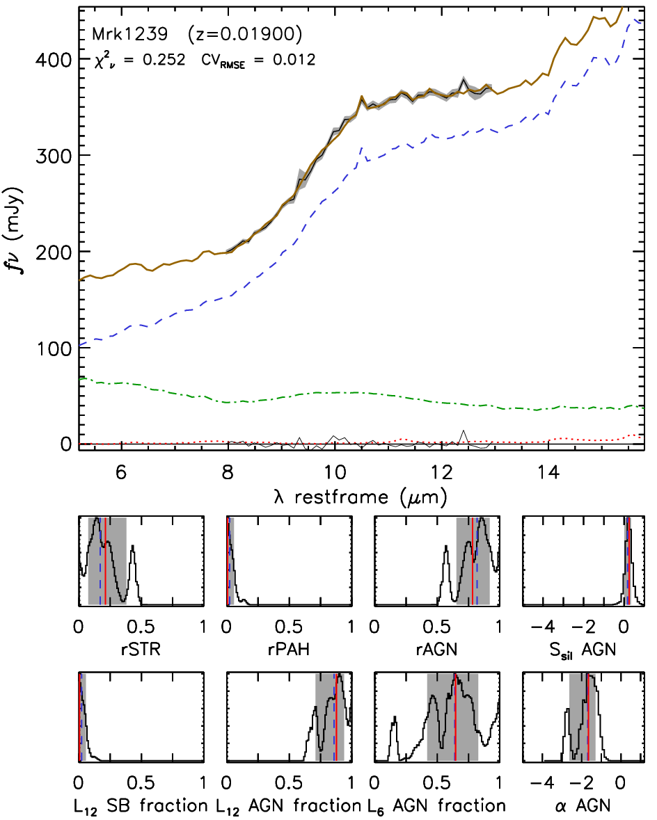
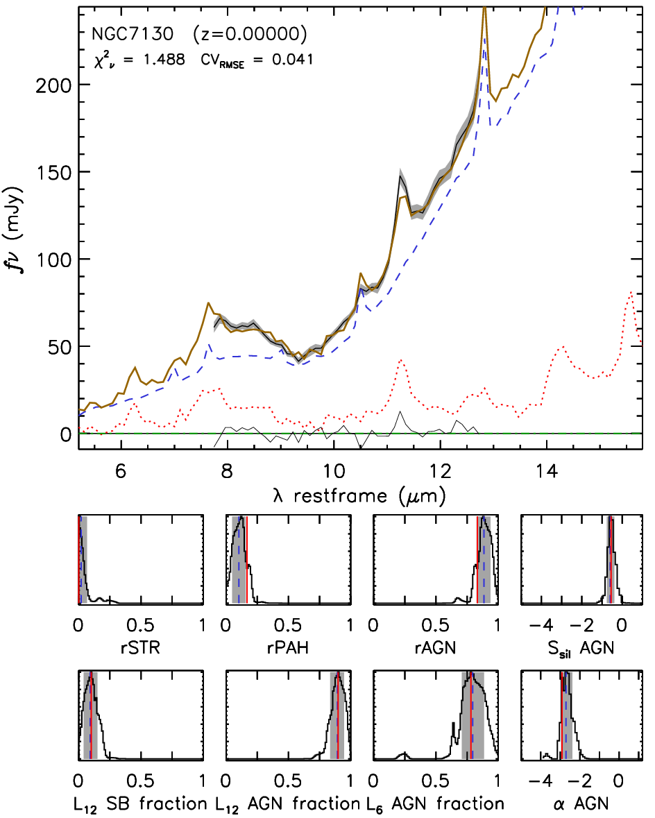
Figure 16: Examples of the output of deblendIRS for Mrk 1239 (Seyfert 1-1.5, left panel), and NGC 7130 (Seyfert 2, right panel). For each example, the top panels show the rest-frame spectrum with the best fitting model (orange), and the three components: stellar (dash-dotted green), PAH (dotted red) and AGN (dashed blue). In the bottom panels deblendIRS shows the PDF for the STR, PAH and AGN emission fraction within the slit ($5-15$ $\mu$m), namely rSTR, rPAH, and rAGN, respectively; the strength of the $9.7\,\mu$m silicate feature ($S_{\rm Sil}$) and the spectral index ($\alpha$, or $\alpha_{\rm MIR}$ in this work notation) in the AGN spectrum ($8.1-12.5\,\mu$m); the fractional contribution within the slit of the AGN to the rest-frame 6 $\mu$m ($L6_{\rm AGN}$) and 12 $\mu$m ($L12_{\rm AGN}$) luminosity; and the fractional contribution of the host galaxy to the rest-frame 12 $\mu$m luminosity ($L12_{\rm SB}$). For the PDFs the solid red line indicates the value for the best fitting decomposition model whereas the dashed blue line indicates the expectation value. The shaded area represents the 16% and 84% percentiles, i.e., the 1$\sigma$ confidence interval.

Appendix

The main output of deblendIRS is the best-fit combination of the stellar, interstellar and AGN components. It also calculates the probability distribution functions (PDF) of the 8 parameters shown in Fig. 16 where we show an example of a Seyfert 1.5 (Mrk 1239) and and example of a Seyfert 2 galaxy (NGC 7130). We refer the reader to Hernán-Caballero et al. (2015) for a full description of deblendIRS.

For the galaxies observed with two instruments, we performed the deblendIRS decomposition for each one of the spectra. In order to select the best one, we compared the values obtained for the AGN spectral index and the AGN silicate strength. For each galaxy we selected the spectrum for which estimated $\alpha_{\rm MIR}$ and $S_{\rm Sil}$ had the smallest 1$\sigma$ confidence interval (16% and 84% percentiles), i.e., the one with smaller error bars in Fig. 17. These in turn are the spectra with the lowest estimated errors. The observed spectrum corresponding to the best-fit is marked in bold in Table 2. From Fig. 17 we can see that for each galaxy the silicate strengths fitted from the different instrument spectra are similar. In the case of the AGN spectral index, for each galaxy the values from the two spectra are mostly compatible within the 1$\sigma$ confidence interval.

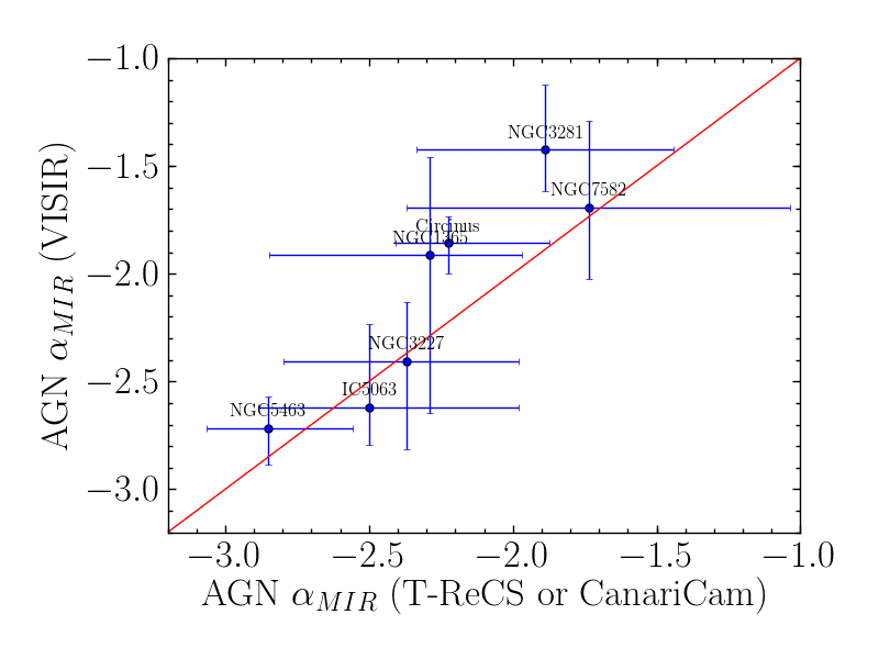
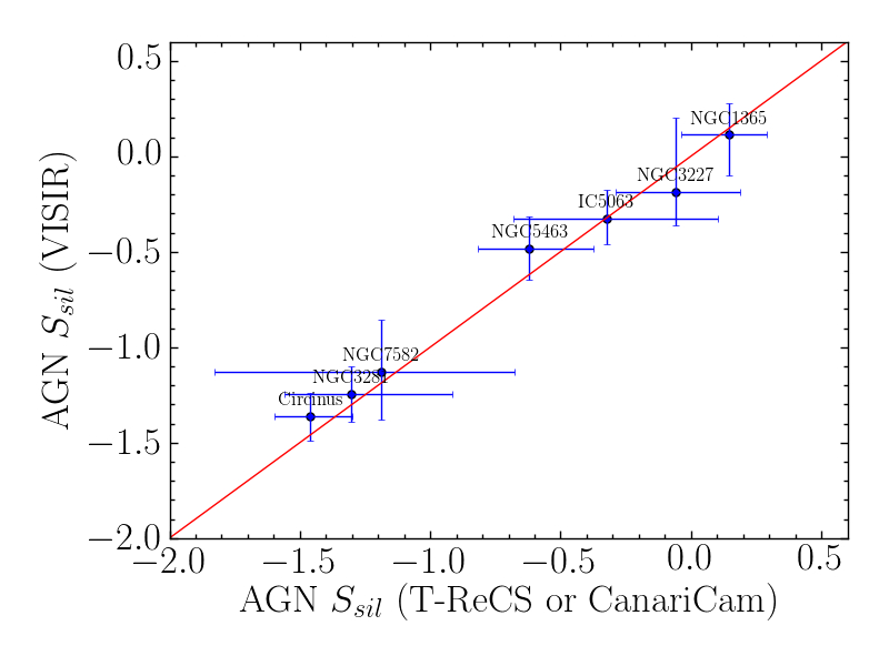
Figure 17: Comparison of the values obtained with deblendIRS for the AGN MIR spectral index (AGN $\alpha_{\rm MIR}$, left panel) and the silicate strength (AGN $S_{\rm Sil}$, right panel) for the galaxies observed with two different instruments. The error bars represent the 1$\sigma$ confidence interval (16% and 84% percentiles). The solid red line is not a fit but it represents the 1:1 relation.

References

- Alonso-Herrero et al. (2001) Alonso-Herrero A., Quillen A. C., Simpson C., Efstathiou A., Ward M. J., 2001, AJ, 121, 1369
- Alonso-Herrero et al. (2011) Alonso-Herrero A., et al., 2011, ApJ, 736, 82
- Alonso-Herrero et al. (2012) Alonso-Herrero A., et al., 2012, MNRAS, 425, 311
- Alonso-Herrero et al. (2014) Alonso-Herrero A., et al., 2014, MNRAS, 443, 2766
- Alonso-Herrero et al. (2016a) Alonso-Herrero A., et al., 2016a, MNRAS, 455, 563
- Alonso-Herrero et al. (2016b) Alonso-Herrero A., et al., 2016b, MNRAS, 463, 2405
- Antonucci (1984) Antonucci R. R. J., 1984, ApJ, 278, 499
- Antonucci (1993) Antonucci R., 1993, ARA&A, 31, 473
- Asmus et al. (2014) Asmus D., Hönig S. F., Gandhi P., Smette A., Duschl W. J., 2014, MNRAS, 439, 1648
- Asmus et al. (2015) Asmus D., Gandhi P., Hönig S. F., Smette A., Duschl W. J., 2015, MNRAS, 454, 766
- Asmus et al. (2016) Asmus D., Hönig S. F., Gandhi P., 2016, ApJ, 822, 109
- Audibert et al. (2017) Audibert A., Riffel R., Sales D. A., Pastoriza M. G., Ruschel-Dutra D., 2017, MNRAS, 464, 2139
- Brightman & Nandra (2011) Brightman M., Nandra K., 2011, MNRAS, 413, 1206
- Burtscher et al. (2013) Burtscher L., et al., 2013, A&A, 558, A149
- Burtscher et al. (2015) Burtscher L., et al., 2015, A&A, 578, A47
- Contini et al. (1998) Contini T., Considere S., Davoust E., 1998, A&AS, 130, 285
- Díaz-Santos et al. (2010) Díaz-Santos T., Alonso-Herrero A., Colina L., Packham C., Levenson N. A., Pereira-Santaella M., Roche P. F., Telesco C. M., 2010, ApJ, 711, 328
- Dullemond & van Bemmel (2005) Dullemond C. P., van Bemmel I. M., 2005, A&A, 436, 47
- Efstathiou & Rowan-Robinson (1995) Efstathiou A., Rowan-Robinson M., 1995, MNRAS, 273, 649
- Elitzur (2012) Elitzur M., 2012, ApJ, 747, L33
- Esquej et al. (2014) Esquej P., et al., 2014, ApJ, 780, 86
- Feltre et al. (2012) Feltre A., Hatziminaoglou E., Fritz J., Franceschini A., 2012, MNRAS, 426, 120
- Fritz et al. (2006) Fritz J., Franceschini A., Hatziminaoglou E., 2006, MNRAS, 366, 767
- Gallimore et al. (2016) Gallimore J. F., et al., 2016, ApJ, 829, L7
- Gandhi et al. (2009) Gandhi P., Horst H., Smette A., Hönig S., Comastri A., Gilli R., Vignali C., Duschl W., 2009, A&A, 502, 457
- García-Bernete et al. (2016) García-Bernete I., et al., 2016, MNRAS, 463, 3531
- García-Burillo et al. (2016) García-Burillo S., et al., 2016, ApJ, 823, L12
- Glasse et al. (1997) Glasse A. C., Atad-Ettedgui E. I., Harris J. W., 1997, in Ardeberg A. L., ed., Proc. SPIEVol. 2871, Optical Telescopes of Today and Tomorrow. pp 1197–1203
- González-Martín et al. (2013) González-Martín O., et al., 2013, A&A, 553, A35
- González-Martín et al. (2015) González-Martín O., et al., 2015, A&A, 578, A74
- Goulding et al. (2012) Goulding A. D., Alexander D. M., Bauer F. E., Forman W. R., Hickox R. C., Jones C., Mullaney J. R., Trichas M., 2012, ApJ, 755, 5
- Granato & Danese (1994) Granato G. L., Danese L., 1994, MNRAS, 268, 235
- Hao et al. (2010) Hao H., et al., 2010, ApJ, 724, L59
- Hatziminaoglou et al. (2015) Hatziminaoglou E., Hernán-Caballero A., Feltre A., Piñol Ferrer N., 2015, ApJ, 803, 110
- Hernán-Caballero et al. (2015) Hernán-Caballero A., et al., 2015, ApJ, 803, 109
- Hönig & Kishimoto (2010) Hönig S. F., Kishimoto M., 2010, A&A, 523, A27
- Hönig & Kishimoto (2017) Hönig S. F., Kishimoto M., 2017, ApJ, 838, L20
- Hönig et al. (2006) Hönig S. F., Beckert T., Ohnaka K., Weigelt G., 2006, A&A, 452, 459
- Hönig et al. (2010) Hönig S. F., Kishimoto M., Gandhi P., Smette A., Asmus D., Duschl W., Polletta M., Weigelt G., 2010, A&A, 515, A23
- Hönig et al. (2013) Hönig S. F., et al., 2013, ApJ, 771, 87
- Houck et al. (2004) Houck J. R., et al., 2004, ApJS, 154, 18
- Ichikawa et al. (2015) Ichikawa K., et al., 2015, ApJ, 803, 57
- Kishimoto et al. (2007) Kishimoto M., Hönig S. F., Beckert T., Weigelt G., 2007, A&A, 476, 713
- Krabbe et al. (2001) Krabbe A., Böker T., Maiolino R., 2001, ApJ, 557, 626
- Krolik & Begelman (1988) Krolik J. H., Begelman M. C., 1988, ApJ, 329, 702
- Lagage et al. (2004) Lagage P. O., et al., 2004, The Messenger, 117, 12
- Levenson et al. (2007) Levenson N. A., Sirocky M. M., Hao L., Spoon H. W. W., Marshall J. A., Elitzur M., Houck J. R., 2007, ApJ, 654, L45
- Levenson et al. (2009) Levenson N. A., Radomski J. T., Packham C., Mason R. E., Schaefer J. J., Telesco C. M., 2009, ApJ, 703, 390
- Lira et al. (2013) Lira P., Videla L., Wu Y., Alonso-Herrero A., Alexander D. M., Ward M., 2013, ApJ, 764, 159
- López-Gonzaga et al. (2016) López-Gonzaga N., Burtscher L., Tristram K. R. W., Meisenheimer K., Schartmann M., 2016, A&A, 591, A47
- Lutz et al. (2004) Lutz D., Maiolino R., Spoon H. W. W., Moorwood A. F. M., 2004, A&A, 418, 465
- Maiolino & Rieke (1995) Maiolino R., Rieke G. H., 1995, ApJ, 454, 95
- Malizia et al. (2012) Malizia A., Bassani L., Bazzano A., Bird A. J., Masetti N., Panessa F., Stephen J. B., Ubertini P., 2012, MNRAS, 426, 1750
- Manske & Henning (1998) Manske V., Henning T., 1998, A&A, 337, 85
- Manske et al. (1998) Manske V., Henning T., Men’shchikov A. B., 1998, A&A, 331, 52
- Marinucci et al. (2012) Marinucci A., Bianchi S., Nicastro F., Matt G., Goulding A. D., 2012, ApJ, 748, 130
- Martínez-Paredes et al. (2017) Martínez-Paredes M., et al., 2017, MNRAS, 468, 2
- Mason et al. (2006) Mason R. E., Geballe T. R., Packham C., Levenson N. A., Elitzur M., Fisher R. S., Perlman E., 2006, ApJ, 640, 612
- Mor & Netzer (2012) Mor R., Netzer H., 2012, MNRAS, 420, 526
- Mor et al. (2009) Mor R., Netzer H., Elitzur M., 2009, ApJ, 705, 298
- Nenkova et al. (2002) Nenkova M., Ivezić Ž., Elitzur M., 2002, ApJ, 570, L9
- Nenkova et al. (2008a) Nenkova M., Sirocky M. M., Ivezić Ž., Elitzur M., 2008a, ApJ, 685, 147
- Nenkova et al. (2008b) Nenkova M., Sirocky M. M., Nikutta R., Ivezić Ž., Elitzur M., 2008b, ApJ, 685, 160
- Netzer (1987) Netzer H., 1987, MNRAS, 225, 55
- Nikutta et al. (2009) Nikutta R., Elitzur M., Lacy M., 2009, ApJ, 707, 1550
- Osterbrock & Martel (1993) Osterbrock D. E., Martel A., 1993, ApJ, 414, 552
- Packham et al. (2005a) Packham C., Telesco C. M., Hough J. H., Ftaclas C., 2005a, in Hidalgo-Gámez A. M., González J. J., Rodríguez Espinosa J. M., Torres-Peimbert S., eds, Revista Mexicana de Astronomia y Astrofisica, vol. 27 Vol. 24, Revista Mexicana de Astronomia y Astrofisica Conference Series. pp 7–12
- Packham et al. (2005b) Packham C., Radomski J. T., Roche P. F., Aitken D. K., Perlman E., Alonso-Herrero A., Colina L., Telesco C. M., 2005b, ApJ, 618, L17
- Phinney (1989) Phinney E. S., 1989, in Meyer F., ed., NATO Advanced Science Institutes (ASI) Series C Vol. 290, NATO Advanced Science Institutes (ASI) Series C. p. 457
- Pier & Krolik (1992) Pier E. A., Krolik J. H., 1992, ApJ, 401, 99
- Polletta et al. (1996) Polletta M., Bassani L., Malaguti G., Palumbo G. G. C., Caroli E., 1996, ApJS, 106, 399
- Radomski et al. (2003) Radomski J. T., Piña R. K., Packham C., Telesco C. M., De Buizer J. M., Fisher R. S., Robinson A., 2003, ApJ, 587, 117
- Ramos Almeida et al. (2009) Ramos Almeida C., et al., 2009, ApJ, 702, 1127
- Ramos Almeida et al. (2011) Ramos Almeida C., et al., 2011, ApJ, 731, 92
- Ramos Almeida et al. (2014) Ramos Almeida C., Alonso-Herrero A., Levenson N. A., Asensio Ramos A., Rodríguez Espinosa J. M., González-Martín O., Packham C., Martínez M., 2014, MNRAS, 439, 3847
- Roche et al. (2006) Roche P. F., Packham C., Telesco C. M., Radomski J. T., Alonso-Herrero A., Aitken D. K., Colina L., Perlman E., 2006, MNRAS, 367, 1689
- Roche et al. (2007) Roche P. F., Packham C., Aitken D. K., Mason R. E., 2007, MNRAS, 375, 99
- Roche et al. (2015) Roche P. F., Alonso-Herrero A., Gonzalez-Martin O., 2015, MNRAS, 449, 2598
- Rowan-Robinson (1995) Rowan-Robinson M., 1995, MNRAS, 272, 737
- Sales et al. (2011) Sales D. A., Pastoriza M. G., Riffel R., Winge C., Rodríguez-Ardila A., Carciofi A. C., 2011, ApJ, 738, 109
- Sales et al. (2013) Sales D. A., Pastoriza M. G., Riffel R., Winge C., 2013, MNRAS, 429, 2634
- Schartmann et al. (2005) Schartmann M., Meisenheimer K., Camenzind M., Wolf S., Henning T., 2005, A&A, 437, 861
- Schartmann et al. (2008) Schartmann M., Meisenheimer K., Camenzind M., Wolf S., Tristram K. R. W., Henning T., 2008, A&A, 482, 67
- Schulz et al. (1999) Schulz H., Komossa S., Schmitz C., Mücke A., 1999, A&A, 346, 764
- Shi et al. (2006) Shi Y., et al., 2006, ApJ, 653, 127
- Siebenmorgen et al. (2015) Siebenmorgen R., Heymann F., Efstathiou A., 2015, A&A, 583, A120
- Sirocky et al. (2008) Sirocky M. M., Levenson N. A., Elitzur M., Spoon H. W. W., Armus L., 2008, ApJ, 678, 729
- Stalevski et al. (2012) Stalevski M., Fritz J., Baes M., Nakos T., Popović L. Č., 2012, MNRAS, 420, 2756
- Stalevski et al. (2016) Stalevski M., Ricci C., Ueda Y., Lira P., Fritz J., Baes M., 2016, MNRAS, 458, 2288
- Stenholm (1994) Stenholm L., 1994, A&A, 290, 393
- Telesco et al. (1998) Telesco C. M., Pina R. K., Hanna K. T., Julian J. A., Hon D. B., Kisko T. M., 1998, in Fowler A. M., ed., Proc. SPIEVol. 3354, Infrared Astronomical Instrumentation. pp 534–544
- Telesco et al. (2003) Telesco C. M., et al., 2003, in Iye M., Moorwood A. F. M., eds, Proc. SPIEVol. 4841, Instrument Design and Performance for Optical/Infrared Ground-based Telescopes. pp 913–922, doi:10.1117/12.458979
- Thompson et al. (2009) Thompson G. D., Levenson N. A., Uddin S. A., Sirocky M. M., 2009, ApJ, 697, 182
- Tristram et al. (2009) Tristram K. R. W., et al., 2009, A&A, 502, 67
- Tueller et al. (2008) Tueller J., Mushotzky R. F., Barthelmy S., Cannizzo J. K., Gehrels N., Markwardt C. B., Skinner G. K., Winter L. M., 2008, ApJ, 681, 113
- Tueller et al. (2010) Tueller J., et al., 2010, ApJS, 186, 378
- Urry & Padovani (1995) Urry C. M., Padovani P., 1995, PASP, 107, 803
- Véron-Cetty & Véron (2010) Véron-Cetty M.-P., Véron P., 2010, A&A, 518, A10
- Wada (2012) Wada K., 2012, ApJ, 758, 66
- Young et al. (2007) Young S., Packham C., Mason R. E., Radomski J. T., Telesco C. M., 2007, MNRAS, 378, 888
- van Bemmel & Dullemond (2003) van Bemmel I. M., Dullemond C. P., 2003, A&A, 404, 1