Bloch theory and spectral gaps
for linearized water waves

Abstract.

The system of equations for water waves, when linearized about equilibrium of a fluid body with a varying bottom boundary, is described by a spectral problem for the Dirichlet – Neumann operator of the unperturbed free surface. This spectral problem is fundamental in questions of stability, as well as to the perturbation theory of evolution of the free surface in such settings. In addition, the Dirichlet – Neumann operator is self-adjoint when given an appropriate definition and domain, and it is a novel but very natural spectral problem for a nonlocal operator. In the case in which the bottom boundary varies periodically, $\{y=-h+b(x)\}$ where $b(x+\gamma)=b(x)$, $\gamma\in\Gamma$ a lattice, this spectral problem admits a Bloch decomposition in terms of spectral band functions and their associated band-parametrized eigenfunctions. In this article we describe this analytic construction in the case of a spatially periodic bottom variation from constant depth in two space dimensional water waves problem, giving a description of the Dirichlet – Neumann operator in terms of the bathymetry $b(x)$ and a construction of the Bloch eigenfunctions and eigenvalues as a function of the band parameters. One of the consequences of this description is that the spectrum consists of a series of bands separated by spectral gaps which are zones of forbidden energies. For a given generic periodic bottom profile $b(x)=\varepsilon\beta(x)$, every gap opens for a sufficiently small value of the perturbation parameter $\varepsilon$.

1. Introduction

This paper concerns the motion of a free surface of fluid over a variable bottom, a problem of significance for ocean dynamics in coastal regions where waves are strongly affected by the topography. There is an extensive literature devoted to the effect of variable depth over surface waves and there are many scaling regimes of interest, including in particular regimes where the typical wavelength of surface waves is assumed to be much longer than the typical lengthscale of the variations of the bathymetry. For purposes of many mathematical studies, the variable bottom topography is assumed either to be periodic, or else to be described by a stationary random ergodic process.

References on the influence of rough bottoms on the free surface include works of Rosales & Papanicolaou [13], Craig et al [2] [3], and Nachbin & Sølna [10], where techniques of homogenization theory are used to obtain effective long wave model equations. The article [4] performs a rigorous analysis of the effect of a rapidly varying periodic bottom in the shallow water regime. Using simultaneously the techniques of homogenization theory and long-wave analysis, a new model system of equations is derived, consisting of the classical shallow water equations that give rise to effective (or homogenized) surface wave dynamics, coupled with a system of nonlocal evolution equations for a periodic corrector term. A rigorous justification for this decomposition is given in [4] in the form of a consistency analysis, in the sense that the constructed approximated solutions satisfy the water wave equations up to a small error term that is controlled analytically. A central issue in this approach is the question of the time of validity of the approximation. It is shown that the result is valid for a time interval of duration $\mathcal{O}(1)$ in the shallow water scaling only if the free surface is not in resonance with the rapidly varying bottom. However resonances are not exceptional. When resonances occur, secular growth of the corrector terms takes place, and this compromises the validity of the approximation, and in particular, a small amplitude, rapidly oscillating bathymetry will affect the free surface at leading order. The motivation for the present study is to develop analytical tools that will be useful in order to address the dynamics of these resonant situations. As a first step, we consider in this paper the water wave system with a periodic bottom profile, linearized near the stationary state, and we develop a Bloch theory for the linearized water wave evolution. This analysis takes the form of a spectral problem for the Dirichlet – Neumann operator of the fluid domain with periodic bathymetry.

The starting point of our analysis is the water wave problem written in its Hamiltonian formulation. Let

$$\mathcal{S}(b,\eta)=\left\{(x,y):x\in\mathbb{R},-h+b(x)<y<\eta(x,t)\right\}$$

be the two-dimensional time-dependent fluid domain where the variable bottom is given by $y=-h+b(x)$, and the free surface elevation by $y=\eta(x,t)$. Following [15] and [5], we pose the problem in canonical variables $(\eta,\xi)$, where $\xi(x)$ is the trace of the velocity potential on the free surface $\{y=\eta(x)\}$. In these variables, the equations of motion for nonlinear free surface water waves are

(1.3) $$\left\{\begin{array}[]{ll}\partial_{t}\eta-G[\eta,b]\xi=0,\\ \partial_{t}\xi+g\eta+\frac{1}{2}\left|\partial_{x}\xi\right|^{2}-\dfrac{\left(G[\eta,b]\xi+\partial_{x}\eta\cdot\partial_{x}\xi\right)^{2}}{2(1+\left|\partial_{x}\eta\right|^{2})}=0~{}.\end{array}\right.$$

The operator $G[\eta,b]$ is the Dirichlet – Neumann operator, defined by

(1.4) $$G[\eta,b]\xi=\sqrt{1+|\partial_{x}\eta|^{2}}\partial_{n}\varphi_{|_{y=\eta}}~{},$$

where $\varphi$ is the solution of the elliptic boundary value problem

(1.5) $$\left\{\begin{array}[]{l}\partial_{x}^{2}\varphi+\partial_{y}^{2}\varphi=0\quad\text{in}\quad{\mathcal{S}}(b,\eta)~{},\\ \varphi_{|_{y=\eta}}=\xi,\qquad\partial_{n}\varphi_{|_{y=-h+b}}=0~{},\end{array}\right.$$

and $g$ is the acceleration due to gravity. In the present article, we consider the system of water wave equations, linearized near a surface at rest and in the presence of periodic bottom. The bottom defined as $y=-h+b(x)$ where $b$ is $2\pi$ - periodic in $x$. We assume $b$ is in $C^{1}(\mathbb{T}^{1})$ where $\mathbb{T}^{1}$ is the periodized interval $[0,2\pi)$. The system (1.3) linearized about the stationary solution $(\eta(x),\xi(x))=(0,0)$ is as follows.

(1.8) $$\left\{\begin{array}[]{ll}\partial_{t}\eta-G[b]\xi=0,\\ \partial_{t}\xi+g\eta=0~{},\end{array}\right.$$

where now, and for the remainder of this article, we denote $G[0,b]$ by $G[b]$. This is an analog of the wave equation, however with the usual spatial Laplacian replaced by the nonlocal operator $G[b]$ whose coefficients are $2\pi$-periodic dependent upon the horizontal spatial variable $x$:

(1.9) $$\partial^{2}_{t}\eta+gG[b]\eta=0~{}.$$

The initial data for the linearized surface displacement $\eta(x,t)$ are

(1.10) $$\eta(x,0)=\eta_{0}(x),\;\;\partial_{t}\eta(x,0)=\eta_{1}(x),\;\;x\in\mathbb{R}~{},$$

these being defined on the whole line.

Bloch decomposition, a spectral decomposition for differential operators with periodic coefficients, is a classical tool to study wave propagation in periodic media. For a relatively recent example, Allaire et al. [1] considered the problem of propagation of waves packets through a periodic medium, where the period is assumed small compared to the size of the envelope of the wave packet. In this work the authors construct solutions built upon Bloch plane waves having a slowly varying amplitude. In a study of Bloch decomposition for the linearized water wave problem over a periodic bed, Yu and Howard [14] use a conformal map that transforms the original fluid domain to a uniform strip. Using this map, they calculate the formal Fourier series for Bloch eigenfunctions. For various examples of bottom profiles, they compute numerically the Bloch eigenfunctions and eigenvalues, from which they identify the spectral gaps and make several observations of their behavior.

The main goal of our work in the present paper is to develop Bloch spectral theory for the Dirichlet – Neumann operator, in analogy with the classical case of partial differential operators with periodic coefficients. This theory constructs the spectrum as a sequence of bands separated by gaps of instability; it serves as a basis for perturbative calculations that gives rise to explicit formulas and rigorous understanding of spectral gaps, and therefore intervals of unstable modes of the linearized water wave problem over periodic bathymetry.

The principle of the Bloch decomposition is to parametrize the continuous spectrum and the generalized eigenfunctions of the spectral problem for $G[b]$ on $L^{2}(\mathbb{R})$ with a family of spectral problems for $G[b]$ on the interval $[0,2\pi)$, with $\theta$-periodic boundary conditions. For this purpose, we construct the Bloch eigenvalues and eigenfunctions of the spectral problem

(1.11) $$G[b]\Phi(x,\theta)=\Lambda(\theta)\Phi(x,\theta)~{},$$

with boundary conditions

(1.12) $$\Phi(x+2\pi,\theta)=\Phi(x,\theta)e^{2\pi i\theta}~{},$$

where $-1/2\leq\theta<1/2$; such behavior is termed to be $\theta$-periodic in $x$. This introduces the band parameter $\theta$.

When the bottom is flat, $b=0$, the Bloch eigenvalues $\Lambda^{(0)}_{n}(\theta)$ are given explicitly in terms of the classical dispersion relation for water waves over a constant depth, namely

(1.13) $$\Lambda^{(0)}_{n}(\theta)=\omega^{2}(n+\theta)=(n+\theta)\tanh(h(n+\theta))$$

for $n\in\mathbb{N}$, and the Bloch parameter $\theta\in\mathbb{S}^{1}$, where $\mathbb{S}^{1}$ is the circle $[-1/2,1/2)$ with periodic continuation. Eigenvalues are simple for $-1/2<\theta<0$ and $0<\theta<1/2$. For half-integer values of $n+\theta$, namely $n+\theta=0,1/2,1\dots$, eigenvalues $\Lambda^{(0)}_{n}(\theta)$ have multiplicity two. If reordered appropriately by their magnitude, the eigenvalues are continuous and periodic in $\theta$ with period $1$. The eigenfunctions $\Phi(x,\theta)$ satisfy the boundary conditions (1.12). With the ordering of the eigenvalues specified above, the eigenfunctions $\Phi_{n}^{(0)}(x,\theta)$ are periodic in $\theta$, again of period $1$.

Just as in the case of Bloch theory for many second order partial differential operators, we find that the presence of the bottom generally results in the splitting of double eigenvalues near such points of multiplicity, creating a spectral gap.

Definition 1.1.

For $\theta\in\mathbb{S}^{1}$ and $b(x)\in C^{(}\mathbb{T}^{1})$ such that $h-b(x)\geq c_{0}>0$, the operator $G_{\theta}[b]$ is defined by

(1.14) $$G_{\theta}[b]=e^{i\theta x}G[b]e^{-i\theta x}.$$

We will show that $G_{\theta}[b]$ maps functions in $H^{1}(\mathbb{T}^{1})$ to $L^{2}(\mathbb{T}^{1})$, in particular it takes $2\pi$-periodic functions into $2\pi$-periodic functions. We will furthermore show that its spectrum on the domain $H^{1}(\mathbb{T}^{1})\subset L^{2}(\mathbb{T}^{1})$ consists of a non-decreasing sequence of eigenvalues

$$\Lambda_{0}(\theta)\leq\Lambda_{1}(\theta)\leq\cdots\leq\Lambda_{n}(\theta)\leq\cdots$$

which are continuous and periodic in $\theta$. The eigenvalues are also continuous in $b$, for $b$ in a $C^{1}$- neighborhood $B_{R}(0)$ of the origin. The corresponding eigenfunctions $\psi_{n}(x,\theta)$ are $2\pi$-periodic in $x$ and periodic in $\theta$ and the corresponding solutions $\Phi_{n}(x,\theta)$ of $G[b]\Phi_{n}(x,\theta)=\Lambda_{n}(\theta)\Phi(x,\theta)$ are $\theta$-periodic. In the case of $(\theta,b)$ such that $\Lambda_{n-1}(\theta)<\Lambda_{n}(\theta)<\Lambda_{n+1}(\theta)$, the eigenvalue $\Lambda_{n}(\theta)$ is simple, and it and eigenfunction $\Phi_{n}(x,\theta)$ are locally analytic in both $\theta$ and $b$.

The spectrum of the Dirichlet – Neumann operator $G[b]$ on the line, namely on the domain $H^{1}(\mathbb{R})\subset L^{2}(\mathbb{R})$, is the union of the ranges of the Bloch eigenvalues $\Lambda_{n}(\theta)$, that is

$$\sigma_{L^{2}(\mathbb{R})}(G[b])=\cup_{n=0}^{+\infty}[\Lambda_{n}^{-},\Lambda_{n}^{+}]$$

where $\Lambda_{n}^{-}=\min_{\theta\in\mathbb{T}^{1}}\Lambda_{n}(\theta)$ and $\Lambda_{n}^{+}=\max_{\theta\in\mathbb{T}^{1}}\Lambda_{n}(\theta)$. It is the analog of the structure of spectral bands and gaps of the Hill’s operator [9]. The ground state $\Lambda_{0}(\theta)$ satisfies $\Lambda_{0}(0)=0$ for any bathymetry $b(x)$, and its corresponding eigenfunction is $\Phi(x,0)=1$.

In Section 4 we give a perturbation analysis of spectral behavior and we compute the gap opening for $b(x)=\varepsilon\beta(x)$, asymptotically as a function of $\varepsilon$. As an example we consider $b(x)=\varepsilon\cos(x)$, in analogy with the case of Matthieu’s equation, and we calculate the asymptotic behavior of the first several spectral gaps. We find that, as in Floquet theory for Hill equation, the first spectral gap obeys $|\Lambda_{0}^{+}-\Lambda_{1}^{-}|=\mathcal{O}(\varepsilon)$. However, in contrast to the case of the Matthieu equation, the second spectral gap only opens at order $|\Lambda_{1}^{+}-\Lambda_{2}^{-}|=\mathcal{O}(\varepsilon^{4})$. In addition, we show that the centre of the gap $\frac{1}{2}(\Lambda_{1}^{-}+\Lambda_{0}^{+})$ is strictly decreasing in $\varepsilon$.

A generic bottom profile $b(x)$ will open all spectral gaps. Clearly, the band endpoints $\Lambda_{n}^{\pm}$ satisfy $\Lambda_{n}^{-}<\Lambda_{n}^{+}$ unless $\partial_{\theta}\Lambda_{n}(\theta)\equiv 0$ which certainly does not occur in a perturbative regime. For sufficiently small generic bathymetric variations $b(x)$, we also know that $\Lambda_{n}^{+}\leq\Lambda_{n+1}^{-}$, which is the case for Hill’s operator, and although we conjecture this to be the case for the Dirichlet – Neumann operator for large general $b(x)$, we do not have a proof of this fact. Furthermore, for Hill’s operator, the band edges $\{\Lambda_{n}^{+},\Lambda_{n+1}^{-}\}_{n\in\mathbb{N}}$ of the $n^{th}$ gap correspond to the $4\pi$ periodic spectrum, while we do not have a proof of the analogous result for the Dirichlet – Neumann operator. The reality condition implies that $\Lambda_{n}(\theta)=\Lambda_{n}(-\theta)$, and therefore for $n$ even, $\partial_{\theta}\Lambda_{n-1}(0)=\partial_{\theta}\Lambda_{n}(0)=0$ when the $n^{th}$ gap opens. The same holds for $\theta=\pm 1/2$ and $n$ odd. The existence of a spectral gap implies that the spectrum is locally simple. Hence the general theory [12][7] of self-adjoint operators implies analyticity of both $\Lambda_{n}(\theta)$ and $\Phi(x,\theta)$. In fact, for $\theta\neq 0,\pm 1/2$, the unperturbed spectrum is simple and the same statement of local analyticity holds for $b(x)\subseteq B_{R}(0)$. Gaps are not guaranteed to remain open as the size of the bottom variations increases, as shown in the numerical simulations performed in [14], Fig.4 (second gap).

2. The Dirichlet – Neumann operator

The goal is to study the spectral problem

(2.1) $$G[b]\Phi(x,\theta)=\Lambda(\theta)\Phi(x,\theta)~{},$$

where $G[b]$ is the Dirichlet – Neumann operator for the fluid domain $\mathcal{S}(b,0)$. We impose $\theta$-periodic boundary conditions

(2.2) $$\Phi(x+2\pi,\theta)=\Phi(x,\theta)e^{2\pi i\theta}$$

for $\theta\in\mathbb{S}^{1}$ the Bloch parameter. It is convenient in Bloch theory to define

(2.3) $$\psi(x,\theta)=e^{-i\theta x}\Phi(x,\theta)$$

to transform the original problem to an eigenvalue problem with periodic boundary conditions. Indeed, condition (2.2) implies that $\psi(x,\theta)$ is periodic in $x$ of period $2\pi$. The spectral problem is now rewritten in conjugated form

(2.4) $$G_{\theta}[b]\psi(x,\theta):=e^{-i\theta x}G[b]e^{i\theta x}\psi(x,\theta)=\Lambda(\theta)\psi(x,\theta)~{}.$$

2.1. Analysis of the Dirichlet – Neumann operator

The following proposition states the basic properties of the Dirichlet – Neumann operator with $\theta$-periodic boundary conditions.

Proposition 2.1.

For each $-1/2\leq\theta<1/2$, the operator $G_{\theta}[b]$ is self-adjoint from $H^{1}(\mathbb{T}^{1})$ to $L^{2}(\mathbb{T}^{1})$ with periodic boundary conditions. It has an infinite sequence of eigenvalues $\Lambda_{0}(\theta)\leq\dots\leq\Lambda_{n}(\theta)\leq\Lambda_{n+1}(\theta)\leq\dots$, which tend to $\infty$ as $n$ tends to $\infty$ in such a way that $\Lambda_{n}(\theta)\sim n/2$.

Writing $D=-i\partial_{x}$, the Dirichlet – Neumann operator $G[b]$ is written as

$$G[b]=G_{0}+DL[b],$$

where $G_{0}=D\tanh(hD)$ is the Dirichlet – Neumann operator with a flat bottom, and $DL[b]$ is the correction due to the presence of the topography. In [2], it was shown that $G[b]=G_{0}+DL[b]$ has a convergent Taylor expansion in powers of $b$, for $b$ in $B_{R}(0)$ of $C^{1}$ and the successive terms can be calculated explicitly. Also,

(2.5) $$DL[b]=-DB[b]A[b]~{},$$

where

$$A[b]f(x)=\int_{\mathbb{R}}e^{ikx}\sinh(b(x)k)\operatorname{sech}(hk)\hat{f}(k)dk$$

(2.6) $$B[b]f(x)=\frac{1}{\pi}\int\frac{\partial_{x^{\prime}}b(x^{\prime})(x^{\prime}-x)+h-b(x^{\prime})}{(x-x^{\prime})^{2}+(b(x^{\prime})-h)^{2}}f(x^{\prime})dx^{\prime}$$

$$\qquad-\frac{1}{2\pi}\int\ln\bigl{(}(x-x^{\prime})^{2}+(h-b(x^{\prime}))^{2}\bigr{)}\tilde{G}[-h+b]f(x^{\prime})dx^{\prime}~{},$$

where $\widetilde{G}[-h+b]$ is the usual Dirichlet – Neumann operator in the domain $\mathcal{S}(b,0)=\{-h+b<y<0\}$ that associates Dirichlet data on the boundary $\{y=-h+b(x)\}$ with Neumann bottom boundary condition at $y=0$, to the normal derivative of the solution to Laplace’s equation on $\{y=-h+b(x)\}$. Because of the special decay properties of the integral kernels for $A[b]$ and $B[b]$, these operators are well defined on periodic and $\theta$-periodic functions. In the following,

$$G_{\theta}[b]=G_{\theta}[0]+M,$$

where we use the notation

(2.7) $$G_{\theta}[0]=e^{-i\theta x}G_{0}e^{i\theta x}$$

$$M=e^{-i\theta x}DL[b]e^{i\theta x}=-\bigl{(}e^{-i\theta x}DB[b]e^{i\theta x}\bigr{)}\bigl{(}e^{-i\theta x}A[b]e^{i\theta x}\bigr{)}~{}.$$

The operators $M$, $DB_{\theta}[b]v=e^{-i\theta x}DB[b]e^{i\theta x}$ and $A_{\theta}[b]=e^{-i\theta x}A[b]e^{i\theta x}$ map $2\pi$-periodic functions to $2\pi$-periodic functions. The operator $G_{\theta}[0]$ is unbounded on $L^{2}(\mathbb{T}^{1})$. It is diagonal in Fourier space variables

$$G_{\theta}e^{ijx}=(j+\theta)\tanh(h(j+\theta))e^{ijx}~{}.$$

In the next proposition, we prove that $G[b]$ preserves the class of $\theta$-periodic functions.

Proposition 2.2.

Given $2\pi$-periodic bottom topography, $b(x+2\pi)=b(x)$, suppose that $\xi(x)\in H^{1}_{loc}(\mathbb{R})$ is a $\theta$-periodic function defined on $\mathbb{R}$, namely that

(2.8) $$\xi(x+2\pi)=e^{2\pi i\theta}\xi(x)~{}.$$

Then the result of application of the Dirichlet – Neumann operator $G[b]\xi(x)$ is also a $\theta$-periodic periodic. That is

(2.9) $$(G[b]\xi)(x+2\pi)=e^{2\pi i\theta}G[b]\xi(x)~{}.$$

Proof.

Let $\varphi(x,y)$ be the harmonic extension of $\xi(x)$ satisfying the bottom boundary conditions $N_{b(x)}\cdot\nabla\varphi(x,y)=0$. By linearity, $e^{2\pi i\theta}\varphi(x,y)$ is the harmonic extension of $e^{2\pi i\theta}\xi(x)$ satisfying the same bottom boundary condition. On the other hand, the harmonic extension of $\xi_{1}(x):=\xi(x+2\pi)$ is $\varphi(x+2\pi,y)$ with the bottom boundary conditions $N_{b(x+2\pi)}\cdot\nabla\varphi(x+2\pi,y)=N_{b(x)}\cdot\nabla\varphi(x+2\pi,y)=0$, due to the periodicity of $b(x)$. By uniqueness of solutions, condition (2.8) implies that $\varphi(x+2\pi,y)=e^{2\pi i\theta}\varphi(x,y)$, from which (2.9) follows, namely

$$e^{2\pi i\theta}(G[b]\xi)(x)=(G[b]\xi_{1})(x)=G[b](e^{2\pi i\theta}\xi(x))~{}.$$

∎

The next statement shows that the operator $M$ is bounded on $L^{2}(\mathbb{T}^{1})$, and in fact is strongly smoothing.

Proposition 2.3.

There exists $R>0$ such that for $b\in B_{R}(0)$, the ball centered at the origin and of radius $R$ of $C^{1}(\mathbb{T}^{1})$ and $f\in L^{2}(\mathbb{T}^{1})$, $Mf$ is also periodic of period $2\pi$, and satisfies the estimate

(2.10) $$\|Mf\|_{L^{2}}\ \leq\ C_{0}(|b|_{C^{1}})\|f\|_{L^{2}}~{},$$

where the constant $C_{0}$ depends on the $C^{1}$-norm of $b$, $C(|b|_{C^{1}})=\mathcal{O}(|b|_{C^{1}})$.

In addition, the operator $M$ is strongly smoothing

(2.11) $$\|Mf\|_{H^{s}}\ \leq\ C_{rs}(|b|_{C^{1}})\|f\|_{H^{-r}}~{}.$$

for all $r,s>0$.

The proof of this proposition is given in Section 5. As a consequence of these two propositions, the operator $G_{\theta}$ defined in (1.14) maps $H^{1}(\mathbb{T}^{1})$ to $L^{2}(\mathbb{T}^{1})$.

2.2. Floquet theory

The spectrum of the Dirichlet – Neumann operator $G[b]$ acting on the domain $H^{1}(\mathbb{R})\subseteq L^{2}(\mathbb{R})$ is real, non-negative, and is composed of bands and gaps. It is the union over $-\frac{1}{2}\leq\theta<\frac{1}{2}$ of the Bloch eigenvalues $\Lambda_{n}(\theta)$, the analog to Bloch theory for the Schrödinger operator.

When $b=0$, the spectrum of $G_{\theta}$ on $L^{2}(\mathbb{T}^{1})$ consists of the Bloch eigenvalues $\Lambda^{(0)}_{n}(\theta)$ which are labeled in order of increasing magnitude. The eigenvalues are periodic in $\theta$ of period one, and are simple when $\theta\neq-\frac{1}{2},0,\frac{1}{2}$. For $\theta=-\frac{1}{2},0,\frac{1}{2}$, the spectrum is double (see Fig.1). Denoting $g_{n}(\theta)=(n+\theta)\tanh(h(n+\theta))$, the eigenvalues and eigenfunctions associated to $G_{\theta}$ are given as follows:

$${\rm For}\ -\frac{1}{2}\leq\theta<0,\quad \Lambda_{2n}^{(0)}(\theta)=g_{-n}(\theta);\ \psi_{2n}^{(0)}(x,\theta)=e^{-inx}~{},$$

$${\rm for}\ 0\leq\theta<\frac{1}{2},\quad \Lambda_{2n}^{(0)}(\theta)=g_{n}(\theta);\ \psi_{2n}^{(0)}(x,\theta)=e^{inx}~{},$$

and

$${\rm for}\ -\frac{1}{2}\leq\theta<0,\quad \Lambda_{2n-1}^{(0)}(\theta)=g_{n}(\theta);\ \psi_{2n-1}^{(0)}(x,\theta)=e^{inx}~{},$$

$${\rm for}\ 0\leq\theta<\frac{1}{2},\quad \Lambda_{2n-1}^{(0)}(\theta)=g_{-n}(\theta);\ \psi_{2n-1}^{(0)}(x,\theta)=e^{-inx}~{}.$$

With this definition, both $\Lambda_{n}^{(0)}$ and $\psi_{n}^{(0)}$ are periodic in $\theta$ with period $1$ and $\Lambda_{n}^{(0)}$ is continuous in $\theta$ while $\psi_{n}^{(0)}$ has discontinuities at $\theta=-\frac{1}{2},0,\frac{1}{2}$.

The goal of our analysis is to show that in the presence of a variable periodic topography, spectral curves which meet when $b=0$ typically separate, creating spectrum gaps corresponding to zones of forbidden energies. For this purpose, assume that the bottom topography is given by $y(x)=-h+b(x)$ where $b$ is a $2\pi$-periodic function in the ball $B_{R}(0)\subseteq C^{1}$, with $\int_{0}^{2\pi}b(x)\,dx=0$, $h-b(x)\geq c_{0}>0$. For our analysis, the circle $\theta\in\mathbb{S}^{1}$ of Floquet exponents is divided into regions in which unperturbed spectra are simple (outer regions), and regions that include the unperturbed multiple spectra (inner regions). To apply the method of continuity, these regions are defined so that they overlap.

Theorem 2.4.

For all $\theta\in(-\frac{3}{8},-\frac{1}{8})\cup(\frac{1}{8},\frac{3}{8})$, the $L^{2}$-spectrum of $G_{\theta}+M$ on the domain $H^{1}(\mathbb{T}^{1})$ is composed of an increasing sequence of eigenvalues $\Lambda_{n}(\theta)$ that are simple, and analytic in $\theta$ and $b\in B_{R}(0)$. The corresponding eigenfunctions $\Psi_{n}(x,\theta)$ are normalized $2\pi$-periodic in $x$, and analytic in $\theta$ and $b\in B_{R}(0)$.

The result in Theorem 2.4 is a direct consequence of the general theory of perturbation of self-adjoint operators [12]. However in Section 3.2, we provide a straightforward alternate proof by means of the implicit function theorem; this approach also serves to motivate the proof of the following result.

Theorem 2.5.

In the neighbourhood of the crossing points $\theta=0,\pm\frac{1}{2}$, i.e for $\theta\in[-\frac{1}{2},-\frac{5}{16})\cup(-\frac{3}{16},\frac{3}{16})\cup(\frac{5}{16},\frac{1}{2}]$, the spectrum of $G_{\theta}+M$ on the domain $H^{1}(\mathbb{T}^{1})$ is composed of an increasing sequence of eigenvalues $\Lambda_{n}(\theta)$ which are continuous in $\theta$. For $\frac{-3}{16}<\theta<\frac{3}{16}$, the lowest eigenvalue $\Lambda_{0}(\theta)$ is simple, and it and the eigenfunction $\Psi_{0}(x,\theta)$ are analytic in $\theta$ and $b$.

Both Theorems 2.4 and 2.5 are local in $\theta$. Their domains of definition overlap on the intervals $\theta\in(-\frac{3}{8},-\frac{5}{16})\cup(-\frac{1}{8},-\frac{3}{16})\cup(\frac{1}{8},\frac{3}{16})\cup(\frac{5}{16},\frac{3}{8})$. By uniqueness, in these intervals the eigenvalues and eigenfunctions agree. Hence they are globally defined periodic functions of $\theta$ in the interval $[-\frac{1}{2},\frac{1}{2})$. We will focus on results concerning the opening of spectral gaps at $\theta=0$ for eigenvalues $\Lambda_{2n-1}(\theta)$ and $\Lambda_{2n}(\theta)$; this is the topic of Section 3.3. The analysis near the double points $\theta=\pm\frac{1}{2}$ is similar.

An illustration of eigenvalues as functions of $\theta$ is given in Figure 1. The left hand side shows the unperturbed first five eigenvalues in the case of a flat bottom labeled in order of magnitude. The right hand side shows these eigenvalues in the presence of a small generic bottom perturbation and the gap openings.

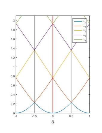
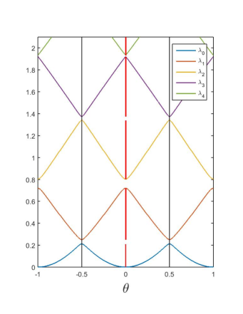
Figure 1. First five eigenvalues in order of magnitude: (left) flat bottom; (right) in the presence of a small generic bottom perturbation. The vertical axis is the $\Lambda$ axis, and the spectra of the operators $G[0]$ and $G[b]$ are represented by the vertical red line and the red intervals, respectively.

3. Gap opening

3.1. A finite-dimensional model of gap opening

We describe now, on a simplified model, the mechanism through which there is the opening of a gap between the two eigenvalues $\Lambda_{2n-1}$ and $\Lambda_{2n}$ near $\theta=0$ in the presence of a periodic bathymetric variation $b(x)$. Denote by $P_{n}$ the orthogonal projection in $L^{2}(\mathbb{T}^{1})$ onto the subspace spanned by $\{e^{inx},e^{-inx}\}$ and decompose the operator $G_{\theta}+M$ as

(3.1) $$G_{\theta}+M =P_{n}(G_{\theta}+M)P_{n}+(I-P_{n})(G_{\theta}+M)P_{n}$$

$$+P_{n}(G_{\theta}+M)(I-P_{n})+(I-P_{n})(G_{\theta}+M)(I-P_{n})~{}.$$

We consider a $2\times 2$ matrix model of (3.1), showing that the presence of a periodic perturbation involving nonzero Fourier coefficients $b_{\pm 2n}$ of the bathymetry $b(x)$ leads to a gap between eigenvalues $\Lambda_{2n-1}(\theta)$ and $\Lambda_{2n}(\theta)$ at $\theta=0$. This model also exhibits how the corresponding eigenfunctions ${\Psi}_{2n-1}$ and $\Psi_{2n}$ are modified. The precise model consists in dropping the three last terms in the rhs of (3.1), reducing $G_{0}+M$ to its first term $P_{n}(G_{\theta}+M)P_{n}$. In addition, we simplify the correction term $M=e^{-i\theta x}DL[b]e^{i\theta x}$ by replacing $DL[b]$ by its one term Taylor series approximation in $b(x)\in C^{1}$, i.e. namely

$$DL_{1}[b]=-D\operatorname{sech}(hD)b(x)D\operatorname{sech}(hD)~{}.$$

Acting on Fourier coefficients of a periodic function $\psi(x)$, the operator $P_{n}(G_{\theta}+e^{-i\theta x}DL_{1}[b]e^{i\theta x})P_{n}$ is represented by the matrix

(3.2) $$A=\begin{pmatrix}g_{n}(\theta)&b_{2n}s_{n}(\theta)s_{n}(-\theta)\\ \overline{b}_{2n}s_{n}(\theta)s_{n}(-\theta)&g_{n}(-\theta)\end{pmatrix}~{},$$

where we have defined $s_{n}(\theta)=(n+\theta)\operatorname{sech}(h(n+\theta))$. We conjugate this matrix to diagonal form as $A=O\Lambda O^{*}$ where

(3.3) $${\Lambda}=\begin{pmatrix}\Lambda_{2n}(\theta)&0\\ 0&\Lambda_{2n-1}(\theta)\end{pmatrix}~{},$$

and where $T=\begin{pmatrix}0&\varphi\\ -\varphi&0\end{pmatrix}$ so that $O=\begin{pmatrix}\cos\varphi&\sin\varphi\\ -\sin\varphi&\cos\varphi\end{pmatrix}=e^{T}=(O^{-1})^{*}$ is a rotation. The eigenvalues $\Lambda_{2n-1}(\theta)\leq\Lambda_{2n}(\theta)$ are explicitly given as

$$\frac{1}{2}\Big{(}g_{n}(\theta)+g_{n}(-\theta)\pm\sqrt{(g_{n}(\theta)-g_{n}(-\theta))^{2}+4|b_{2n}|^{2}s_{n}(\theta)^{2}s_{n}(-\theta)^{2}}\Big{)}~{}.$$

Assuming $b_{2n}\neq 0$, the eigenvalues split near $\theta=0$, and in particular $\Lambda_{2n}(0)-\Lambda_{2n-1}(0)=\mathcal{O}(|b_{2n}|)$. The corresponding eigenfunctions are ${\Psi}_{2n-1}(\theta)=O^{*}\begin{pmatrix}1\\ 0\end{pmatrix}$ and ${\Psi}_{2n}(\theta)=O^{*}\begin{pmatrix}0\\ 1\end{pmatrix}$, where $\varphi\sim 0$ for $\theta>0$ and $\varphi\sim\pi/2$ for $\theta<0$. The eigenvalues $\Lambda_{2n-1}(\theta)$, $\Lambda_{2n}(\theta)$ are Lipschitz continuous in $\theta$. For nonzero $b_{2n}$, both the matrix $O$ and the eigenvalues $\Lambda_{2n-1}(\theta)$, $\Lambda_{2n}(\theta)$ are continuous and indeed even locally analytic.

3.2. Perturbation of simple eigenvalues

We now take up the spectral problem for the full Dirichlet – Neumann operator $G[b]$. Consider values of the parameter $\theta$ in the interval $\frac{1}{8}<\theta<\frac{3}{8}$, for which $\Lambda_{j}^{(0)}(\theta)=g_{j}(\theta)$ is a simple eigenvalue for all $j$. With no loss of generality, suppose that $j=2n$ even (for $j$ odd and $\theta>0$ the only change has to do with the indexing, as is the case of $\theta<0$). By analogy with finite dimensional problem, we seek a conjugacy that when described in terms of the Fourier transform, will reduce the operator $G_{\theta}+M$ to a matrix operator whose off-diagonal entries are zero in the $n^{th}$ row and column. Specifically for the $n^{th}$ eigenvalue, we seek a transformation $O=e^{T}$ parametrized by operators $T$ satisfying $T^{*}=-T$, such that in acting on Fourier series the matrix $e^{-T}(G_{\theta}+M)e^{T}$ will be block diagonal. For this purpose, use the orthogonal projection $P_{n}$ onto the span of the Fourier mode $e^{inx}$ in $L^{2}(\mathbb{T}^{1})$, and decompose the operator $e^{-T}(G_{\theta}+M)e^{T}$ as

(3.4) $$e^{-T}(G_{\theta}+M)e^{T}=P_{n}e^{-T}(G_{\theta}+M)e^{T}P_{n}+(I-P_{n})e^{-T}(G_{\theta}+M)e^{T}P_{n}$$

$$\qquad+P_{n}e^{-T}(G_{\theta}+M)e^{T}(I-P_{n})+(I-P_{n})e^{-T}(G_{\theta}+M)e^{T}(I-P_{n})~{}.$$

We are seeking $T$ that is an anti-Hermitian operator such that the block off-diagonal components of (3.4) satisfy

(3.5) $$(I-P_{n})e^{-T}(G_{\theta}+M)e^{T}P_{n}+P_{n}e^{-T}(G_{\theta}+M)e^{T}(I-P_{n})=0~{}.$$

The existence of such $T$ will follow from the implicit function theorem [11], applied in a space of operators. Define $F:\>(T,M)\;\rightarrow\;F(T,M)$, where

(3.6) $$F_{1}(T,M)=P_{n}e^{-T}(G_{\theta}+M)e^{T}(I-P_{n})~{},\;\;F_{2}(T,M)=F_{1}^{*}(T,M)~{},$$

(3.7) $$F(T,M)=F_{1}(T,M)+F_{2}(T,M)~{}.$$

The goal is to solve $F(T,M)=0$, describing $T$ as a function of $M$ in appropriate functional spaces. We look for $T$ a solution of (3.5) restricted to the space of anti-Hermitian operators with the additional mapping property that

(3.8) $$T(P_{n}L^{2})\subseteq(I-P_{n})L^{2},\quad{\rm{and}}\quad T((I-P_{n})L^{2})\subseteq P_{n}L^{2}~{}.$$

The following analysis is performed in Fourier space coordinates, which is to say in a basis given in terms of Fourier series. Denote $h^{r}$ the space of $2\pi$-periodic functions in $H^{r}$, represented in Fourier series coordinates. Alternately using Plancherel, this characterizes $\psi\in h^{r}$ by its sequence of Fourier coefficients;

$$h^{r}=\{(\psi_{l})_{l\in\mathbb{Z}}\ :\ \sum_{l\in\mathbb{Z}}\langle l\rangle^{2r}|\psi_{l}|^{2}<+\infty\}~{},$$

where as usual we write $\langle l\rangle=\sqrt{2}(|l|^{2}+1)^{1/2}$.

In Fourier space variables, operators have a matrix representation in the basis $\{\frac{1}{\sqrt{2\pi}}e^{ikx}\}_{k\in\mathbb{Z}}$, defined by

$$Ae^{ilx}=\sum_{j\in\mathbb{Z}}A_{jl}e^{ijx}~{}.$$

For the most part, we will be concerned with the Hermitian and anti-Hermitian operators. A scale of operator norms for Hermitian (and anti-Hermitian) operators represented in Fourier coordinates is given by

$$\|A\|_{r}=\sup_{j}\bigl{(}\sum_{l\in\mathbb{Z}}|A_{jl}|\langle j-l\rangle^{r}\bigr{)}~{}.$$

This norm quantifies the off-diagonal decay of the matrix elements of $A$. The identical expression for a norm is used for anti-hermitian operators $T:h^{r}\to h^{r}$, while for a general operator $Y$ we need to use

$$\|Y\|_{r}:=\Bigl{(}\sup_{j}\sum_{k}|Y_{jk}|\langle j-k\rangle^{r}\Bigr{)}^{1/2}\Bigl{(}\sup_{k}\sum_{j}|Y_{jk}|\langle j-k\rangle^{r}\Bigr{)}^{1/2}.$$

The space of linear operators from the Sobolev space $h^{r}$ to itself that have finite $r$-norm is denoted by ${\mathcal{L}}_{r}$. It is a Banach space with respect to this norm. The space of Hermitian symmetric operators with finite $r$-norm is denoted by ${\mathcal{H}}_{r}$ while the space of anti-Hermitian symmetric operators with finite $r$-norm is denoted by ${\mathcal{A}}_{r}$. When $r=0$, this norm dominates the usual operator norm on $\ell^{2}$, while for $r>0$ the expression gives a norm which is a bound for $A\ :\ h^{r}\to h^{r}$. One notes that this is indeed a proper operator norm, such that $\|M\psi\|_{h^{r}}\leq\|M\|_{r}\|\psi\|_{h^{r}}$. In fact if $\|M\|_{r}<+\infty$ this same inequality holds when considering $M:h^{s}\to h^{s}$ for any $0\leq s\leq r$.

Proposition 3.1.

Taking $b\in B_{R}(0)\subseteq C^{1}(\mathbb{T}^{1})$, then for all $r\geq 0$, the Fourier representation of the operator $M$ defined in (2.7) satisfies

$$\|M\|_{r}=\sup_{j}\bigl{(}\sum_{l\in\mathbb{Z}}|M_{jl}|\langle j-l\rangle^{r}\bigr{)}\leq C_{r}(|b|_{C^{1}})=\mathcal{O}(|b|_{C^{1}})~{}.$$

This bound follows directly from Proposition 2.3.

We also must consider unbounded operators on sequence spaces, for instance $A:h^{r}\to h^{r-1}$, for which the operator norm that we use is given by

$$\|A\|_{h^{r}\to h^{r-1}}:=\Bigl{(}\sup_{j}\sum_{k}|A_{jk}|\frac{1}{\langle j\rangle}\langle j-k\rangle^{r}\Bigr{)}^{1/2}\Bigl{(}\sup_{k}\sum_{j}|A_{jk}|\frac{1}{\langle j\rangle}\langle j-k\rangle^{r}\Bigr{)}^{1/2}.$$

Denote the space of such operators by $\mathcal{H}_{h^{r}\to h^{r-1}}$. It is worth the remark that our diagonal operator $G_{\theta}$ satisfies $\|G_{\theta}\|_{h^{r}\to h^{r-1}}<+\infty$.

Proposition 3.2.

For any operators $A:h^{r}\to h^{r-1}$ and $B:h^{r}\to h^{r}$ the operator composition $AB$ satisfies

$$\|AB\|_{h^{r}\to h^{r-1}}\leq\|A\|_{h^{r}\to h^{r-1}}\|B\|_{r}$$

The same estimate holds for the operator composition $BA$.

Proof: We note that in our proof, we principally encounter Hermitian and/or anti-Hermitian operators $A$ and $B$. Their product does not share these properties of symmetry however, and we must use the general expression for the norm for operators $h^{r}\to h^{r}$. Take $A$ and $B$ as in the proposition, where we suppose that $\|A\|_{h^{r}\to h^{r-1}}$ and $\|B\|_{r}$ are finite, and calculate

$$\|AB\|_{h^{r}\to h^{r-1}} =\Bigl{(}\sup_{j}\sum_{k}\bigl{|}\sum_{l}A_{jl}B_{lk}\bigr{|}\frac{1}{\langle j\rangle}\langle j-k\rangle^{r}\Bigr{)}^{1/2}\Bigl{(}\sup_{k}\sum_{j}\bigl{|}\sum_{l}A_{jl}B_{lk}\bigr{|}\frac{1}{\langle j\rangle}\langle j-k\rangle^{r}\Bigr{)}^{1/2}$$

$$\leq\Bigl{(}\sup_{j}\sum_{k}\sum_{l}|A_{jl}|\frac{1}{\langle j\rangle}\langle j-l\rangle^{r}|B_{lk}|\langle l-k\rangle^{r}\Bigl{(}\frac{\langle j-k\rangle^{r}}{\langle j-l\rangle^{r}\langle l-k\rangle^{r}}\Bigr{)}\Bigr{)}^{1/2}$$

$$\quad\times\Bigl{(}\sup_{k}\sum_{j}\sum_{l}|A_{jl}|\frac{1}{\langle j\rangle}\langle j-l\rangle^{r}|B_{lk}|\langle l-k\rangle^{r}\Bigl{(}\frac{\langle j-k\rangle^{r}}{\langle j-l\rangle^{r}\langle l-k\rangle^{r}}\Bigr{)}\Bigr{)}^{1/2}~{}.$$

Since

$$\frac{\langle j-k\rangle^{r}}{\langle j-l\rangle^{r}\langle l-k\rangle^{r}}\leq 1~{},$$

then the rhs is bounded by $\|A\|_{h^{r}\to h^{r-1}}\|B\|_{r}$. ∎

In addition, the family of operators $F$ defined in (3.7) satisfies the mapping properties (3.8); these properties define a linear subspace $\mathcal{Q}_{h^{r}\to h^{r-1}}\subseteq{\mathcal{H}}_{h^{r}\to h^{r-1}}$. The operator $M\in{\mathcal{H}}_{r}$ defined in (2.7) is a bounded Hermitian symmetric operator, as expressed in Proposition 2.1 and Proposition 3.1. We seek a solution $T$ of (3.5) in Fourier coordinates, where $T\in\mathcal{A}_{r}$, which also satisfies the mapping property (3.8). The set of anti-Hermitian operators satisfying (3.8) is a linear subspace $\mathcal{P}_{r}\subseteq\mathcal{A}_{r}$ (it is not however closed under operator composition).

Describing $T$ in terms of its matrix elements in Fourier variables, because of the property (3.8), $Te^{inx}=\sum_{l\in\mathbb{Z}\backslash\{n\}}T_{ln}e^{ilx}$, while for $j\neq n$ then $Te^{ijx}=T_{nj}e^{inx}=-\overline{T}_{jn}e^{inx}$. Thus the operator $T$, identified by its matrix elements $T_{nl}=-\overline{T}_{ln}$, is nonzero only in the $n^{th}$ row and column, and its operator norm is given by

$$\|T\|_{r}=\sum_{l\neq n}|T_{nl}|\langle n-l\rangle^{r}~{}.$$

Similarly, the operator $M$ is defined in terms of its matrix elements by its action on Fourier modes, $Me^{ilx}=\sum_{j\in\mathbb{Z}}M_{jl}e^{ijx}$.

Theorem 3.3.

[Simple eigenspace perturbation]. There exists $\rho>0$ and a continuous map

(3.9) $$M\in B_{\rho}(0)\subseteq{\mathcal{H}}_{r}\rightarrow T\in{\mathcal{P}}_{r}$$

such that $F(T(M),M)=0$  . Furthermore, $T(M)$ is analytic with respect to $M$. For $b\in B_{R}(0)\subseteq C^{1}(\mathbb{T}^{1})$, the operator $M=M(b)$ is continuous with respect to $b$, and $M(0)=0$. Therefore, there exists $0<\rho_{1}<R$ such that for $b\in B_{\rho_{1}}(0)\subseteq C^{1}(\mathbb{T}^{1})$, $M(b)\in B_{\rho}(0)$ and there is a solution $T=T(b)$ of (3.9). Furthermore, $M$ is analytic in $b$, therefore $T$ is analytic in $b$.

The result is that $e^{T(M)}$ is a unitary transformation that conjugates the operator $(G_{\theta}+M)$ to diagonal on the eigenspace associated with the eigenvalues $\Lambda_{2n-1}(\theta)$ and $\Lambda_{2n}(\theta)$.

The proof of Theorem 3.3 is an application of the implicit function theorem, for which we need to verify the hypotheses. As a starting point, clearly $F(0,0)=0$ since $G_{\theta}$ is diagonal in a Fourier basis. We proceed to verify the relevant properties of the mapping $F$ and its Jacobian derivative $\partial_{T}F$. This is the object of Lemma 3.4.

Lemma 3.4.

Let $r\geq 1$. (i) For $(T,M)\in U$ an open subset of ${\mathcal{P}}_{r}\times{\mathcal{H}}_{r}$ containing $(0,0)$, $F(T,M)\in\mathcal{Q}_{h^{r}\to h^{r-1}}$, which is continuous in $M$, and $C^{1}$ in $T$.

(ii) The Fréchet derivative $\partial_{T}F(0,0)$ at $(T,M)=0$ is invertible, namely for $N\in\mathcal{Q}_{h^{r}\to h^{r-1}}$, there is a unique $V\in\mathcal{P}_{r}$ such that

$$\partial_{T}F(0,0)V=N~{}.$$

Proof.

We will show that $F(T,M)$ has the required smoothness and invertibility properties as an element of $\mathcal{Q}_{h^{r}\to h^{r-1}}$, in order to invoke the implicit function theorem. Firstly, the function $F(T,M)\in{\mathcal{Q}}_{h^{r}\to h^{r-1}}$ is built of operators with the following properties: Firstly the operator $G_{\theta}$ maps $h^{r}$ to $h^{r-1}$, and it is diagonal in the Fourier basis. The operator $e^{T}\in{\mathcal{L}}_{r}$, in fact it is unitary; also, $Me^{T}\in{\mathcal{L}}_{r}$. Because $G_{\theta}\in\mathcal{L}_{h^{r}\to h^{r-1}}$, then $G_{\theta}e^{T}\in{\mathcal{L}}_{h^{r}\to h^{r-1}}.$ We have

$$e^{-T}(G_{\theta}+M)e^{T}\in{\mathcal{H}}_{h^{r}\to h^{r-1}}~{},$$

therefore

$$F:=P_{n}[e^{-T}(G_{\theta}+M)e^{T}](I-P_{n})+(*)\in{\mathcal{Q}}_{h^{r}\to h^{r-1}}~{},$$

where $(*)$ denotes the Hermitian conjugate of the prior expression. This functional property dictates the choice of sequence spaces above.

Secondly, we use the series expansion of exponential of operators

(3.10) $$e^{T_{1}}-e^{T_{2}}=\sum\frac{1}{m!}(T_{1}^{m}-T_{2}^{m})~{},$$

and furthermore

$$T_{1}^{m}-T_{2}^{m} =T_{1}^{m-1}(T_{1}-T_{2})+T_{1}^{m-2}(T_{1}-T_{2})T_{2}+....+(T_{1}-T_{2})T_{2}^{m-1}$$

$$=\sum_{p=0}^{m-1}T_{1}^{p}(T_{1}-T_{2})T_{2}^{m-p-1}~{}.$$

Consequently the following operator norm inequality holds:

$$e^{T_{1}}-e^{T_{2}}=\sum_{m}\frac{1}{m!}\sum_{p=0}^{m-1}T_{1}^{p}(T_{1}-T_{2})T_{2}^{m-p-1}~{},$$

$$\|e^{T_{1}}-e^{T_{2}}\|_{r}\leq\sum_{m=1}^{\infty}\frac{1}{(m-1)!}a^{m-1}\|T_{1}-T_{2}\|_{r}=e^{a}\|T_{1}-T_{2}\|_{r}~{},$$

where $a=\max(\|T_{1}\|_{r},\|T_{2}\|_{r})$.

To verify the continuity of $F$ with respect to $T$, compute the difference

$$F (T_{1},M)-F(T_{2},M)$$

$$= P_{n}\bigl{(}e^{-T_{1}}(G_{\theta}+M)e^{T_{1}}-e^{-T_{2}}(G_{\theta}+M)e^{T_{2}}\bigr{)}(I-P_{n})+(*)$$

(3.11) $$= P_{n}\bigl{(}e^{-T_{1}}G_{\theta}(e^{T_{1}}-e^{T_{2}})+(e^{-T_{1}}-e^{-T_{2}})G_{\theta}e^{T_{2}}\bigr{)}(I-P_{n})$$

$$+P_{n}\bigl{(}e^{-T_{1}}M(e^{T_{1}}-e^{T_{2}})+(e^{-T_{1}}-e^{-T_{2}})Me^{T_{2}}\bigr{)}(I-P_{n})+(*)~{},$$

where again $(*)$ is the Hermitian conjugate. Both $(e^{T_{1}}-e^{T_{2}})$ and $e^{T_{2}}$ are bounded in the operator $r$-norm and since $r\geq 1$ thus

$$\|e^{-T_{1}}G_{\theta}(e^{T_{1}}-e^{T_{2}})\|_{{h^{r}\to h^{r-1}}} \leq\|e^{-T_{1}}G_{\theta}\|_{{h^{r}\to h^{r-1}}}e^{a}\|T_{1}-T_{2}\|_{r}$$

$$\leq\|e^{-T_{1}}\|_{r}\|G_{\theta}\|_{{h^{r}\to h^{r-1}}}e^{a}\|T_{1}-T_{2}\|_{r}~{},$$

which is the result of Lipschitz continuity. Similarly

$$\|(e^{-T_{1}}-e^{-T_{2}})G_{\theta}e^{T_{2}}\|_{{h^{r}\to h^{r-1}}} \leq e^{a}\|T_{1}-T_{2}\|_{r}\|G_{\theta}\|_{{h^{r}\to h^{r-1}}}\|e^{-T_{2}}\|_{r}~{}.$$

Analogous estimates hold for the term involving $M$;

$$\|e^{-T_{1}}M(e^{T_{1}}-e^{T_{2}})+(e^{-T_{1}}-e^{-T_{2}})Me^{-T_{2}}\|_{{h^{r}\to h^{r-1}}}$$

$$\qquad\leq e^{a}\|M\|_{r}\bigl{(}\|e^{-T_{1}}\|_{r}+\|e^{-T_{2}}\|_{r}\bigr{)}\|T_{1}-T_{2}\|_{r}~{}.$$

The operator $F(T,M)$ is affine linear in $M$, thus the estimate of continuity is even more straightforward, namely

$$\|F(T,M_{1})-F(T,M_{2})\|_{{h^{r}\to h^{r-1}}} =\|P_{n}(e^{-T}(M_{1}-M_{2})e^{T})(I-P_{n})+(*)\|_{h^{r}\to h^{r-1}}$$

$$\leq C\|M_{1}-M_{2}\|_{r}~{}.$$

We now address the continuity of the Fréchet derivative of $F$ with respect to $T$. For this purpose, we write

$$\partial_{T}F(T,M)V=P_{n}(\partial_{T}e^{-T})V(G_{\theta}+M)e^{T}(I-P_{n})+P_{n}e^{-T}(G_{\theta}+M)(\partial_{T}e^{T})V(I-P_{n})+(*)$$

and compute

$$(\partial_{T}e^{T})V=\sum_{m=1}^{\infty}\frac{1}{m!}\sum_{p=0}^{m-1}T^{p}VT^{m-p-1}.$$

(3.12) $$(\partial_{T_{1}}e^{T_{1}})V-(\partial_{T_{2}}e^{T_{2}})V=\sum_{m=1}^{\infty}\frac{1}{m!}\sum_{p=0}^{m-1}(T_{1}^{p}VT_{1}^{m-p-1}-T_{2}^{p}VT_{2}^{m-p-1})$$

$$=\sum_{m=1}^{\infty}\frac{1}{m!}\Big{(}\sum_{p=1}^{m-1}(T_{1}^{p}-T_{2}^{p})VT_{1}^{m-p-1}\Big{)}+\sum_{p=0}^{m-2}T_{2}^{p}V(T_{1}^{m-p-1}-T_{2}^{m-p-1})~{}.$$

Let $a=\max(\|T_{1}\|_{r},\|T_{2}\|_{r})$, then $\|T_{1}^{p}-T_{2}^{p}\|_{r}\leq pa^{p-1}\|T_{1}-T_{2}\|_{r}$,

$$\|\sum_{p=0}^{m-1}(T_{1}^{p}VT_{1}^{m-p-1}-T_{2}^{p}VT_{2}^{m-p-1})\|_{r}\leq \sum_{p=0}^{m-1}pa^{p-1}\|T_{1}-T_{2}\|_{r}a^{m-p-1}\|V\|_{r}~{}.$$

Thus the first term in the rhs of (3.12) is bounded by

$$\|T_{1}-T_{2}\|_{r}\|V\|_{r}\sum_{m}\frac{1}{m!}a^{m-2}\sum_{p=1}^{m-1}p=\|T_{1}-T_{2}\|_{r}\|V\|_{r}\sum_{m}\frac{1}{m!}a^{m-2}\frac{m(m-1)}{2}$$

$$\qquad=\frac{1}{2}e^{a}\|T_{1}-T_{2}\|_{r}\|V\|_{r}~{}.$$

The second term of the rhs of (3.12) has a similar bound. We combine this estimate with the bounds on $G_{\theta}$ and $M$ to obtain the continuity of $\partial_{T}F(T,M)$ with respect to $T$.

We now verify that $\partial_{T}F(0,0)$ is invertible as a mapping of linear operators from $\mathcal{P}_{r}$ to $\mathcal{Q}_{r}$ that satisfy (3.8). Since $\partial_{T}e^{T}|_{T=0}V=V$, then

$$\partial_{T}F(0,0)V=P_{n}[G_{\theta},V](I-P_{n})+(*).$$

Posing the equation

(3.13) $$\bigl{(}P_{n}[G_{\theta},V](I-P_{n})+(*)\bigr{)}_{\pm nl}=N_{nl}~{},\qquad l\neq n~{},$$

given $N\in{\color[rgb]{0,0,1}\mathcal{Q}_{h^{r}\to h^{r-1}}}$ we solve for $V\in\mathcal{P}_{r}$.

We have an explicit inverse expression for $V$ from the fact that $G_{\theta}$ is diagonal, namely

$$V_{jk}=\begin{cases}&\displaystyle{\frac{N_{jn}}{g_{\theta}(j)-g_{\theta}(n)}}~{},\quad j\not=n~{},\quad k=n~{},\\ &\displaystyle{\frac{N_{nk}}{g_{\theta}(n)-g_{\theta}(k)}}~{},\quad j=n~{},\quad k\not=n~{},\\ &0\qquad\qquad\qquad\quad\hbox{\rm otherwise}~{}.\end{cases}$$

The support properties of $V$ follow from this expression, as does the anti-Hermitian property. Because of eigenvalue separation for $j,k\not=n$ and because of the linear growth property of the dispersion relation $g_{\theta}(k)$, we have a lower bound on the denominator

$$|g_{\theta}(j)-g_{\theta}(n)|\geq\frac{1}{C}\langle j-n\rangle~{}.$$

The fact that $V\in{\mathcal{P}}_{r}\subseteq{\mathcal{A}}_{r}$ follows from an estimate of the $r$-operator norm.

$$\|V\|_{r} =\sup_{j}\sum_{k}|V_{jk}|\langle j-k\rangle^{r}$$

(3.14) $$=\max\Bigl{(}\sup_{j\not=n}|V_{jn}|\langle j-n\rangle^{r}~{},~{}\sum_{k\not=n}|V_{nk}|\langle n-k\rangle^{r}\Bigr{)}$$

$$\leq C\max\Bigl{(}\sup_{j\not=n}|N_{jn}|\langle j-n\rangle^{r-1}~{},~{}\sum_{k\not=n}|N_{nk}|\langle n-k\rangle^{r-1}\Bigr{)}~{}.$$

To finish the argument we observe that, for fixed $n$, the quantity $\langle j-n\rangle$ has a lower bound

$$\langle j-n\rangle\geq C_{1}(n)\langle j\rangle~{}.$$

Therefore, in the expression (3.14), we have

$$\|V\|_{r} \leq C\max\Bigl{(}\sup_{j\not=n}|N_{jn}|\langle j-n\rangle^{r}\frac{1}{\langle j-n\rangle}~{},~{}\sum_{k\not=n}|N_{nk}|\langle n-k\rangle^{r}\frac{1}{\langle k-n\rangle}\Bigr{)}$$

$$\leq C\max\Bigl{(}\sup_{j\not=n}|N_{jn}|\frac{1}{\langle j\rangle}\langle j-n\rangle^{r}~{},~{}\sum_{k\not=n}|N_{nk}|\frac{1}{\langle k\rangle}\langle n-k\rangle^{r}\Bigr{)}$$

$$\leq C\|N\|_{{h^{r}\to h^{r-1}}}~{}.$$

This proves that $(\partial_{T}F(0,0))^{-1}:{\mathcal{Q}}_{{h^{r}\to h^{r-1}}}\to{\mathcal{P}}_{r}$ is bounded. ∎

Choosing the operator $T$ as in Theorem 3.3, we now have the decomposition

(3.15) $$e^{-T}(G_{\theta}+M)e^{T}= P_{n}e^{-T}(G_{\theta}+M)e^{T}P_{n}$$

$$+(I-P_{n})e^{-T}(G_{\theta}+M)e^{T}(I-P_{n})~{}$$

in which the $n$th row and column are both identically zero except for the coefficient $\Lambda_{2n}(\theta)$ on the diagonal. Therefore

$$e^{-T}(G_{\theta}+M)e^{T}\delta_{n}=\Lambda_{2n}(\theta)\delta_{n}~{},$$

where $\delta_{n}$ is the Kronecker symbol, $\delta_{n}(j)=0$ $j\neq n,\delta_{n}(n)=1$. Since $P_{n}$ is the projection on the mode $e^{inx}$, an expression for the eigenfunction in space variables is given by $\psi_{2n}(x,\theta)=\sum_{l\in\mathbb{Z}}(e^{T})_{ln}e^{ilx}$, so that

(3.16) $$(G_{\theta}+M)\psi_{2n}(x,\theta)=\Lambda_{2n}\psi_{2n}(x,\theta)~{}.$$

Furthermore, the transformation $e^{T}$ is unitary, so that $\|\psi_{2n}(x,\theta)\|_{\ell^{2}}=1$. That is, the function $\psi_{2n}(x,\theta)$ is the normalized eigenfunction of the operator $(G_{\theta}+M)$ associated to the eigenvalue $\Lambda_{2n}(\theta)$. In addition, since $\|T\|_{r}<+\infty$, the Fourier series expansion of the eigenfunction is localized close to the exponential $e^{inx}$, in that $\delta_{n}-\hat{\psi}_{2n}(l)\leq C_{n}\langle l\rangle^{-r}$. This is the expression for eigenfunctions and associated eigenvalues in the case of simple spectrum. The analysis of $\psi_{2n-1}$ is identical.

3.3. Perturbation of double eigenvalues

The ground state eigenvalue $\Lambda_{0}(\theta)$ is simple in the interval $-\frac{3}{8}<\theta<\frac{3}{8}$ and therefore is also governed by the general theory of self adjoint operators, as mentioned above, or alternatively by our construction of the previous section.

For $1\leq n\in\mathbb{N}$, we focus on the $n^{th}$ spectral gap. We perform a perturbation analysis of spectral subspaces associated with double or near-double eigenvalues $\Lambda_{2n-1}(\theta)$ and $\Lambda_{2n}(\theta)$. Denote $P_{n}$ the projection on the subspace of $L^{2}(\mathbb{T}^{1})$ spanned by $\{e^{inx},e^{-inx}\}$ and define the function $F(T,M)$ as in (3.7) and (3.6). Analogously, define the space of operators respecting the tw0-dimensional range of the projection $P_{n}$ to be ${\mathcal{P}}_{r}$ and ${\mathcal{Q}}_{h^{r}\to h^{r-1}}$.

Theorem 3.5.

[Perturbation of eigenspaces of double eigenvalues]. There exists $\rho>0$ and a continuous map

(3.17) $$M\in B_{\rho}(0)\subseteq{\mathcal{H}}_{r}\rightarrow T\in{\mathcal{P}}_{r}$$

such that $F(T(M),M)=0$  . Furthermore, $T(M)$ is analytic with respect to $M$. For $b\in B_{R}(0)\subseteq C^{1}(\mathbb{T}^{1})$, the operator $M=M(b)$ is continuous with respect to $b$, and $M(0)=0$. Therefore, there exists $0<\rho_{1}<R$ such that for $b\in B_{\rho_{1}}(0)\subseteq C^{1}(\mathbb{T}^{1})$, $M(b)\in B_{\rho}(0)$ and there is a solution $T=T(b)$ of (3.17). Furthermore, $M$ is analytic in $b$, therefore $T$ is analytic in $b$.

The proof of this theorem is similar to the one presented for a simple eigenvalue and relies on the implicit function theorem. We present only the steps in the proof of Lemma 3.4 that need to be modified.

The operator $T$ is such that $T^{*}=-T$, this is to say $T_{\pm nl}=-\overline{T}_{l(\pm n)}$, and the mapping property (3.8) of $T$, which is expressed in terms of the Fourier series basis elements as the properties that $Te^{\pm inx}=\sum_{l\neq\pm n}T_{l(\pm n)}e^{ilx}$, and for $l\neq\pm n$ then $Te^{ilx}=\sum_{\pm n}T_{(\pm n)l}e^{\pm inx}$. In particular, the nonzero entries of $T_{\pm nl}$ are only for indices $\pm n,l\neq n$. The operator norm is defined in the usual way as

$$\|T\|_{r}=\sup_{\pm n}\Bigl{(}\sum_{l}|T_{(\pm n)l}|\langle l\mp n\rangle^{r}\Bigr{)}~{}.$$

When checking the hypotheses for the application of the implicit function theorem, the only point that is necessary to be verified is that the operator $\partial_{T}F(0,0)$ is invertible. To this aim, the solution of equation (3.13) in this case is explicitly

$$V_{(\pm n)l}=\frac{N_{(\pm n)l}}{g_{\pm n}(\theta)-g_{l}(\theta)}~{}$$

for all $l\neq\pm n$. Since for $-\frac{3}{8}<\theta<\frac{3}{8}$ and for $l\neq\pm n$ there is a lower bound on the rhs, namely

$$|{g_{\pm n}(\theta)-g_{l}(\theta)}|>\alpha\langle l\mp n\rangle~{},$$

for any integer $l\neq\pm n$. It is again clear that for $N\in{\mathcal{Q}}_{h^{r}\to h^{r-1}}\subseteq{\mathcal{H}}_{h^{r}\to h^{r-1}}$, the solution $V$ gives an operator that satisfies $V\in{\mathcal{P}}_{r}\subseteq{\mathcal{A}}_{r}$.

We note that the eigenvalues themselves are not analytic in $b$, at least not uniformly in $b$ and in $\theta$ in neighborhoods of double points. This is exhibited in the model of Section 3. But the spectral subspace spanned by $\{\psi_{\pm}\}$is analytic, a common state of affairs in the theory of eigenvalue perturbation in the case of spectrum with varying multiplicity.

4. Perturbation theory of spectral gaps

In this section, we provide a perturbative calculation of the gap created near $\theta=0$ between the eigenvalues $\Lambda_{2n-1}(\theta)$ and $\Lambda_{2n}(\theta)$ in the presence of periodic bathymetry $b(x)$. For clarity of the perturbation computation, we make the substitution $b(x)=\varepsilon\beta(x)$, and continue the discussion as a perturbation calculation in $\varepsilon$.

The first step is to calculate the operator $T$ perturbatively by solving the equation

$$P_{n}e^{-T}(G_{\theta}+M)e^{T}(I-P_{n})+(*)=0~{}.$$

Following this, we calculate the eigenvalues $\Lambda_{2n-1}(\theta)$ and $\Lambda_{2n}(\theta)$ of the $2\times 2$ matrix $P_{n}e^{-T}(G_{\theta}+M)e^{T}P_{n}$ and their corresponding eigenfunctions $\Psi_{2n-1},\Psi_{2n}$. Our calculation provides the eigenfunctions $\psi_{2n-1}=e^{T}\Psi_{2n-1}$ and $\psi_{2n}=e^{T}\Psi_{2n}$ of $G_{\theta}+M$ that are associated to $\Lambda_{2n-1}(\theta)$ and $\Lambda_{2n}(\theta)$.

4.1. Expansion of the operator $T$

Using the Taylor expansion of the Dirichlet – Neumann operator in powers of the bottom variations as calculated in [2], write

$$M=\sum_{p\geq 1}\varepsilon^{p}M_{p}~{}.$$

We seek the anti-Hermitian operator $T$ in the form

$$T=\sum_{p\geq 1}\varepsilon^{p}T_{p}~{}.$$

Proposition 4.1.

The coefficients $T_{p}$ in the series expansion of $T$ are given recursively.

Proof.

Writing the exponentials $e^{\pm T}$ in terms of a formal expansion in $\varepsilon$,

$$e^{T}=I+\sum_{s\geq 1}\varepsilon^{s}T_{+}^{(s)},\qquad e^{-T}=I+\sum_{s\geq 1}\varepsilon^{s}T_{-}^{(s)}~{},$$

we have $T_{\pm}^{(s)}$ computed in terms of $T_{p}$ as

(4.1) $$T_{\pm}^{(s)}=\sum_{j=1}^{s}\frac{(\pm 1)^{j}}{j!}\Bigl{(}\sum_{p_{1}+..+p_{j}=s\atop 1\leq p_{1},\cdots,p_{j}\leq s-(j-1)}T_{p_{1}}\cdots T_{p_{j}}\Bigr{)}~{}.$$

In particular

(4.2) $$T_{\pm}^{(s)} =\pm T_{s}+\sum_{j=2}^{s}\frac{(\pm 1)^{j}}{j!}\Bigl{(}\sum_{p_{1}+..+p_{j}=s\atop 1\leq p_{1},...,p_{j}\leq s-(j-1)}T_{p_{1}}\cdots T_{p_{j}}\Bigr{)}$$

$$:=\pm T_{s}+h_{\pm}^{(s)}(T_{1},\cdots,T_{s-1})~{}.$$

Expand the product

$$e^{-T}(G_{\theta} +M)e^{T}=(I+\sum_{s\geq 1}\varepsilon^{s}T_{-}^{(s)})(G_{\theta}+\sum_{p\geq 1}\varepsilon^{p}M_{p})(I+\sum_{l\geq 1}\varepsilon^{l}T_{+}^{(l)})$$

(4.3) $$= G_{\theta}+\sum_{q\geq 1}\varepsilon^{q}(T_{-}^{(q)}G_{\theta}+G_{\theta}T_{+}^{(q)})+\sum_{q\geq 1}\varepsilon^{q}M_{q}$$

$$\quad+\sum_{q\geq 2}\varepsilon^{q}\sum_{q_{1}+q_{3}=q\atop 1\leq q_{1},q_{3}<q}T_{-}^{(q_{1})}G_{\theta}T_{+}^{(q_{3})}+\sum_{q\geq 2}\varepsilon^{q}\sum_{q_{1}+q_{2}+q_{3}=q\atop 0\leq q_{1},q_{3}<q;1\leq q_{2}<q}T_{-}^{(q_{1})}M_{q_{2}}T_{+}^{(q_{3})}~{}.$$

Apply the projections $P_{n}$ and $I-P_{n}$ to the right and left of (4.1) respectively, and set to zero term of order $q$ ($q\geq 1$),

$$P_{n}(T_{-}^{(q)}G_{\theta}+G_{\theta}T_{+}^{(q)})(I-P_{n})=-P_{n}M_{q}(I-P_{n})$$

(4.4) $$-P_{n}\Big{(}\sum_{q_{1}+q_{3}=q\atop 1\leq q_{1},q_{3}<q}T_{-}^{(q_{1})}G_{\theta}T_{+}^{(q_{3})}+\sum_{q_{1}+q_{2}+q_{3}=q\atop 0\leq q_{1},q_{3}<q;1\leq q_{2}<q}T_{-}^{(q_{1})}M_{q_{2}}T_{+}^{(q_{3})}\Big{)}(I-P_{n})~{}.$$

Isolating $T_{q}$ in the lhs, we get

$$P_{n}[G_{\theta},T_{q}](I-P_{n})=-P_{n}M_{q}(I-P_{n})-P_{n}(h_{-}^{(q)}G_{\theta}+G_{\theta}h_{+}^{(q)})(I-P_{n})$$

(4.5) $$-P_{n}\Big{(}\sum_{q_{1}+q_{3}=q\atop 1\leq q_{1},q_{3}\leq q}T_{-}^{(q_{1})}G_{\theta}T_{+}^{(q_{3})}+\sum_{q_{1}+q_{2}+q_{3}=q\atop 0\leq q_{1},q_{3}<q,\ 1\leq q_{2}<q}T_{-}^{(q_{1})}M_{q_{2}}T_{+}^{(q_{3})}\Big{)}(I-P_{n})~{}.$$

The latter equation for $T_{q}$ has the form

$$P_{n}[G_{\theta},T_{q}](I-P_{n})=P_{n}N_{q}(I-P_{n})~{},$$

where the rhs is defined to be the rhs of (4.1), it depends on all the previous $T_{p}$, $1\leq p\leq q-1$, and its solution is given explicitly by

(4.6) $$(T_{q})_{(\pm n)l}=\frac{(N_{q})_{(\pm n)l}}{g_{\pm n}(\theta)-g_{l}(\theta)}~{},\,\ell\neq\pm n,$$

with the property that $(T_{q})_{l(\pm n)}=-(\overline{T_{q}})_{(\pm n)l}$ and $T_{jk}=0$ otherwise. In particular, for $q=1$, we have

(4.7) $$P_{n}[G_{\theta},T_{1}](I-P_{n}) =-P_{n}M_{1}(I-P_{n})$$

$$(I-P_{n})[G_{\theta},T_{1}]P_{n} =-(I-P_{n})M_{1}P_{n}~{}.$$

∎

Lemma 4.2.

The matrix coefficients of the operator $M_{p}$ are polynomials of order $p$ in $\beta_{k}$, the Fourier coefficients of $\beta$,

$$(M_{p})_{jl}=\sum_{k_{j}\in\mathbb{Z}}m_{p}(k_{1},....,k_{p})\beta_{k_{1}}.....\beta_{k_{p}}$$

where $m_{p}(k_{1},...,k_{p})$ is nonzero only when $k_{1}+...+k_{p}=j-l$.

The matrix coefficients of the operator $T_{p}$ satisfy a similar constraint

$$(T_{p})_{jl}=\sum_{k_{j}\in\mathbb{Z}}t_{p}(k_{1},...,k_{p})\beta_{k_{1}}...\beta_{k_{p}}$$

where $t_{p}(k_{1},...,k_{p})$ is nonzero only when $k_{1}+...+k_{p}=j-l$.

The proof of this lemma is by induction, first using the recursion formula for the operator $M$, as described in [2, Appendix], and then using formula (4.2) and (4.6) for $T$.

We conclude this section by stating the first three terms of the expansion of $T$. For $\ell\neq\pm n$,

(4.8) $$[T_{1},G_{\theta}]_{\pm n\ell}=(M_{1})_{\pm n\ell}$$

$$[T_{2},G_{\theta}]_{\pm n\ell}=(M_{2}+[M_{1},T_{1}])_{\pm n\ell}$$

$$[T_{3},G_{\theta}]_{\pm n\ell}=(M_{3}+[M_{2},T_{1}]+[M_{1},T_{2}]+\frac{1}{3}[T_{1},[T_{1},M_{1}]])_{\pm n\ell}~{}.$$

4.2. Eigenvalue expansion

Define the $2\times 2$ matrix coefficient

(4.9) $$A(\theta,\varepsilon)=P_{n}e^{-T}(G_{\theta}+M)e^{T}P_{n}.$$

We compute the two eigenvalues $\Lambda_{2n-1}(\theta)$ and $\Lambda_{2n}(\theta)$ perturbatively, and thus give conditions for the opening of the $n^{th}$ spectral gap. The order at which the gap opens depends on the Fourier coefficients of $\beta(x)$. Using the expansion of $T$, we find

$$P_{n}e^{-T}(G_{\theta}+M )e^{T}P_{n}=P_{n}G_{\theta}P_{n}+\varepsilon P_{n}M_{1}P_{n}$$

(4.10) $$+\varepsilon^{2}P_{n}\Big{(} \frac{1}{2}[T_{1},[T_{1},G_{\theta}]]+M_{2}+[M_{1},T_{1}]\Big{)}P_{n}$$

$$+\varepsilon^{3}P_{n}\Big{(} \frac{1}{2}[T_{1},[T_{2},G_{\theta}]]+\frac{1}{2}[T_{2},[T_{1},G_{\theta}]]+M_{3}$$

$$+[M_{2},T_{1}]+[M_{1},T_{2}]+\frac{1}{2}[T_{1},[T_{1},M_{1}]]\Big{)}P_{n}+\mathcal{O}(\varepsilon^{4})~{}.$$

From the Taylor expansion of $G[b]$ in powers of $b$ (see Appendix of [2]), we have

$$M_{1} =-e^{-i\theta x}D\operatorname{sech}(hD)\,\beta\,D\operatorname{sech}(hD)e^{i\theta x}$$

$$M_{2} =-e^{-i\theta x}D\operatorname{sech}(hD)\,\beta\,D\tanh(hD)\,\beta(x)\,D\operatorname{sech}(hD)e^{i\theta x}$$

$$M_{3} =e^{-i\theta x}D\operatorname{sech}(hD)\ \Big{(}-\frac{1}{6}\beta^{3}D^{2}+\frac{1}{2}\beta^{2}D\beta$$

$$\qquad-\beta D\tanh(hD)\beta D\tanh(hD)\beta\Big{)}\,D\operatorname{sech}(hD)e^{i\theta x}$$

$$M_{4} =-e^{-i\theta x}D\operatorname{sech}(hD)\Big{(}\frac{1}{2}\beta^{2}D^{2}\beta D\tanh(hD)\beta-\frac{1}{6}\beta D\tanh(hD)\beta^{3}D^{2}$$

$$\qquad+\frac{1}{2}\beta D\tanh(hD)\beta^{2}D^{2}\beta-\frac{1}{6}\beta^{3}D^{3}\tanh(hD)\beta$$

$$\qquad-\beta D\tanh(hD)\beta D\tanh(hD)\beta D\tanh(hD)\Big{)}\,D\operatorname{sech}(hD)e^{i\theta x}~{}.$$

Recalling the notations $g_{k}\theta)=(k+\theta)\tanh(h(k+\theta))$ and $s_{k}(\theta)=(k+\theta)\operatorname{sech}(h(k+\theta))$, we have

(4.11) $$A_{1}:=P_{n}M_{1}P_{n}=\begin{pmatrix}0&-\beta_{2n}s_{n}(\theta)s_{n}(-\theta)\\ -\overline{\beta}_{2n}s_{n}(\theta)s_{n}(-\theta)&0\end{pmatrix},$$

where $A=\sum_{p\geq 0}\varepsilon^{p}A_{p}$. Under the condition that $\beta_{2n}\neq 0$, the $n{{}^{th}}$ gap occurs for $\theta=0$, and the size of the gap is of order $\mathcal{O}(\varepsilon)$, approximated by the difference of the two eigenvalues of the above matrix. This recovers the prediction given by the $2\times 2$ model of Section 3.1. Indeed, computing $A_{1}$ close to the value $\theta=0$, the spectral gap is approximately given by

(4.12) $$\Lambda_{2n}(0)-\Lambda_{2n-1}(0)\sim 2\varepsilon s_{n}^{2}(0)|\beta_{2n}|~{}.$$

If $\beta_{2n}=0$, we may pass to the next term in the expansion. Returning to eq. (4.2), the term of order $\mathcal{O}(\varepsilon^{2})$ reduces to

$$P_{n}\Big{(}\frac{1}{2}[T_{1},[T_{1},G_{\theta}]]+M_{2}+[M_{1},T_{1}]\Big{)}P_{n}.$$

The eigenvalues $\Lambda_{2n-1}(\theta)$ and $\Lambda_{2n}(\theta)$ are approximated at order $\mathcal{O}(\varepsilon^{2})$ by the eigenvalues of the matrix

$$\sum_{k=0}^{2}\varepsilon^{k}A_{k}=\begin{pmatrix}g_{n}(\theta)+\varepsilon^{2}a_{n,n}&\varepsilon^{2}a_{-n,n}\\ \varepsilon^{2}\overline{a}_{-n,n}&g_{-n}(\theta)+\varepsilon^{2}a_{-n,-n}\\ \end{pmatrix}$$

where for $k=\pm n,j=\pm n$, the matrix coefficients of $A_{2}$ are

$$a_{j,k}(\theta)=\left(M_{2}\right)_{jk}+\frac{1}{2}\sum_{\ell\neq\pm n}\left(M_{1}\right)_{j\ell}\left(T_{1}\right)_{\ell k}-\left(T_{1}\right)_{j\ell}\left(M_{1}\right)_{\ell k}~{}.$$

From (4.2)

$$\left(M_{1}\right)_{jk}(\theta) =-s_{j}(\theta)s_{k}(\theta)\beta_{j-k}$$

$$\left(M_{2}\right)_{jk}(\theta) =-\sum_{p\in\mathbb{Z}}s_{j}(\theta)\beta_{j-k-p}g_{k+p}(\theta)\beta_{p}s_{k}(\theta)$$

$$\left(T_{1}\right)_{(\pm n)\ell}(\theta) =\frac{\left(M_{1}\right)_{\pm n,\ell}(\theta)}{g_{\ell}(\theta)-g_{\pm n}(\theta)}=\frac{s_{\pm n}(\theta)s_{\ell}(\theta)\beta_{\pm n-\ell}}{g_{\pm n}(\theta)-g_{\ell}(\theta)}~{}.$$

Explicitly,

$$a_{n,n} =-s_{n}^{2}(\theta)\Big{(}\sum_{k}|\beta_{k}|^{2}g_{k+n}(\theta)-\sum_{l\neq\pm n}\frac{s_{l}^{2}(\theta)|\beta_{n-l}|^{2}}{g_{n}(\theta)-g_{l}(\theta)}\Big{)}~{},$$

$$a_{-n,-n} =-s_{-n}^{2}(\theta)\Big{(}\sum_{k}|\beta_{k}|^{2}g_{k-n}(\theta)-\sum_{l\neq\pm n}\frac{s_{l}^{2}(\theta)|\beta_{n+l}|^{2}}{g_{-n}(\theta)-g_{l}(\theta)}\Big{)}~{},$$

$$a_{n,-n} =-s_{-n}(\theta)s_{n}(\theta)\sum_{k}g_{-k}(\theta)\beta_{n+k}{\beta}_{n-k}$$

$$\quad+\frac{1}{2}s_{n}(\theta)s_{-n}(\theta)\Big{(}\sum_{l\neq\pm n}{\beta}_{n-l}\beta_{l+n}s_{l}^{2}(\theta)(\frac{1}{g_{n}(\theta)-g_{l}(\theta)}+\frac{1}{g_{-n}(\theta)-g_{l}(\theta)})\Big{)}~{},$$

$$a_{-n,n} =\overline{a_{n,-n}}~{}.$$

In a neighborhood of $\theta=0$, one has $g_{n}(\theta)-g_{-n}(\theta)=\mathcal{O}(\theta)$ and $s_{n}(\theta)+s_{-n}(\theta)=\mathcal{O}(\theta)$, so that the terms on the diagonal of $A(\theta)$ satisfy $A_{n,n}(\theta)-A_{-n,-n}(\theta)=\mathcal{O}(\theta)$. Thus, at $\theta=0$, using that $A_{1}=0$, we find that

$$\Lambda_{2n}(0)-\Lambda_{2n-1}(0) =2\varepsilon^{2}|a_{n,-n}|+\mathcal{O}(\varepsilon^{3})$$

where

(4.13) $$a_{n,-n}(0) =-s_{n}(0)^{2}\sum_{l\neq\pm n}\beta_{n-l}\beta_{n+l}(-g_{l}(0)+\frac{s_{l}^{2}(0)}{g_{n}(0)-g_{l}(0)})$$

$$=-s_{n}(0)^{2}\sum_{l\neq\pm n}\beta_{n-l}\beta_{n+l}\frac{l^{2}-g_{n}(0)g_{l}(0)}{g_{n}(0)-g_{l}(0)}~{}.$$

As long as the function $\beta(x)$ describing the bathymetry has nonzero Fourier coefficients $\beta_{l}$ such that for some $l\not=\pm n$ both $\beta_{l\pm n}\not=0$, then this quantity has the possibility to be nonvanishing. In any case it is generically nonzero. In this situation, the above expression gives a description of the asymptotic size of the $n^{th}$ gap opening at order $\mathcal{O}(\varepsilon^{2})$.

Proposition 4.3.

The matrix coefficients of $A(\theta,\varepsilon)$ defined in (4.9) satisfy

(i) $A_{n,n}(0,\varepsilon)=A_{-n,-n}(0,\varepsilon)$ and it is real.

(ii) $A_{n,-n}(0,\varepsilon)=\overline{A}_{-n,n}(0,\varepsilon)$ due to the Hermitian character. A necessary condition for a gap to open under perturbation in $\varepsilon$ is that $A_{n,-n}\neq 0$.

(iii) Let $\mathcal{K}=\{k_{j}\in\mathbb{Z},\ \beta_{k_{j}}\neq 0\}:=\mathcal{K}(\beta)$, the set of Fourier indices corresponding to nonzero coefficients of $\beta(x)$. Suppose that, for all $p\leq q$, and for every sum of integers $\sum_{j=1}^{p}k_{j}=n$, one of the $k_{j}$ does not belong to $\mathcal{K}$. Then there is an upper bound of the $n^{th}$ gap opening

$$|\Lambda_{n}^{-}-\Lambda_{n-1}^{+}|\leq C\varepsilon^{q+1}~{}.$$

(iv) $A(0,\varepsilon)$ is analytic in $\varepsilon$. Thus, it is determined by its Taylor series in $\varepsilon$. If $\frac{\partial^{q}}{\partial\varepsilon^{q}}A_{n,-n}(0,0)=0$ for all $q$, then $A_{n,-n}(0,\varepsilon)=0$ for all $\varepsilon$. In this case, the eigenvalues of $A(0,\varepsilon)$ are double, that is the $n^{th}$ gap remains closed.

Proof.

We study the case of an even numbered gap. The odd numbered gaps are similar. $\frac{\partial^{p}}{\partial\varepsilon^{p}}A_{n,-n}(0,0)$ is the $p^{th}$ Taylor coefficient of the matrix coefficient of $A$. It satisfies the conclusion of Lemma 4.2. It is a polynomial of order $p$ in the Fourier coefficients $\beta_{k}$ :

$$(A_{p})_{n,-n}=\sum a_{p}(k_{1},....,k_{p})\beta_{k_{1}}....\beta_{k_{p}}$$

where $k_{1}+\cdots+k_{p}=2n$. Under the hypothesis (iii), if $p\leq q$, then $(A_{p})_{n,-n}=0$.

The proof of (iv) follows from Theorem 3.3 and the analyticity properties of $M$ with respect to $b$. ∎

4.3. Examples

When $b(x)=\varepsilon\cos(x)$, the first gap occurs for $\theta=\pm 1/2$ and is of order $\mathcal{O}(\varepsilon)$ indeed by (4.12).

$$\Lambda_{1}^{-}-\Lambda_{0}^{+}=g_{0}(\frac{1}{2})2|s_{0}(\frac{1}{2})|^{2}|\beta_{1}|\varepsilon=\frac{1}{4}\operatorname{sech}^{2}(\frac{h}{2})\varepsilon~{}.$$

We are also able to calculate analytically the deviation of the centre. We find that

(4.14) $$\frac{1}{2}(\Lambda_{1}^{-}+\Lambda_{0}^{+})=-\ \varepsilon^{2}\frac{s_{0}^{2}(\frac{1}{2})(g_{0}^{2}(\frac{1}{2})-\frac{9}{4})}{4(g_{0}(\frac{1}{2})-g_{1}(\frac{1}{2}))}+\mathcal{O}(\varepsilon^{3}).$$

It is straightforward to check that this quantity is negative, showing that the centre of the gap is strictly decreasing with $\varepsilon$. Hence for increasing $\varepsilon$ the gap centre is transposed, or downshifted, to lower frequency. This is an analytical verification of Figure 2b of reference [14].

The second gap occurs at $\theta=0$. We find that for $n=1$ the coefficient $a_{n,-n}$ of (4.13) vanishes. We have remarked above that this is in contrast with the case of Matthieu’s equation. Calculating the expansion further and using (4.8) we find that

$$A_{3}=P_{n}\Big{(}\frac{1}{2}[M_{2},T_{1}]+\frac{1}{2}[M_{1},T_{2}]+M_{3}\Big{)}P_{n}$$

and that $A_{3}(0)$ is a multiple of the identity, and in particular the off-diagonal terms satisfy $(A_{3})_{1,-1}=0$, thus not contributing to the formation of a spectral gap. Continuing the perturbation calculation,

$$A_{4}=P_{n}\Big{(} M_{4}-[T_{1},M_{3}]-[T_{2},M_{2}]+\frac{1}{2}[T_{1},[T_{1},M_{2}]]-[T_{3},M_{1}]$$

$$-\frac{1}{6}[T_{1},[T_{1},[T_{1},M_{1}]]]+\frac{1}{2}[T_{1},[T_{2},M_{1}]]+\frac{1}{2}[T_{2},[T_{1},M_{1}]]$$

$$+\frac{1}{24}[T_{1},[T_{1},[T_{1},[T_{1},G_{\theta}]]]]$$

$$+\frac{1}{2}[T_{2},[T_{2},G_{\theta}]]+\frac{1}{2}[T_{1},[T_{3},G_{\theta}]]+\frac{1}{2}[T_{3},[T_{1},G_{\theta}]]\Big{)}P_{n}$$

which can be simplified using (4.8) to

$$A_{4}=P_{n}\Big{(}M_{4}-\frac{1}{2}[T_{1},M_{3}]-\frac{1}{2}[T_{2},M_{2}]-\frac{1}{2}[T_{3},M_{1}]+\frac{1}{24}[T_{1},[T_{1},[T_{1},M_{1}]]]\Big{)}P_{n}.$$

where for $\theta=0$,

$$(M_{4})_{1,-1}=-\frac{1}{3}s_{1}(0)s_{-1}(0)g_{2}(0)\beta_{1}^{3}\beta_{-1}=\frac{1}{48}s_{1}(0)^{2}g_{2}(0)$$

$$([T_{1},M_{3}])_{1,-1}=(T_{1})_{1,2}(M_{3})_{2,-1}-(M_{3})_{1,-2}(T_{1})_{-2,-1}$$

$$\qquad=-\frac{1}{48}s_{2}^{2}(0)s_{1}(0)^{2}\frac{1}{g_{2}(0)-g_{1}(0)}$$

$$([T_{2},M_{2}])_{1,-1}=(T_{2})_{1,-3}(M_{2})_{-3,-1}-(M_{2})_{1,3})T_{2})_{3,-1}=0$$

$$([T_{3},M_{1}])_{1,-1}=(T_{3})_{1,-2}(M_{1})_{-2,-1}-(M_{1})_{1,2}(T_{3})_{2,-1}$$

$$\qquad=\frac{1}{48}s_{1}(0)^{2}s_{2}^{2}(0)\frac{1}{g_{2}(0)-g_{1}(0)}$$

$$([T_{1},[T_{1},[T_{1},M_{1}]]])_{1,-1}=0~{}.$$

Using this lengthy but straightforward calculation, the off-diagonal entries $(A_{4})_{1,-1}=(\overline{A_{4}})_{-1,1}$ of the matrix $A_{4}$, are given by

$$(A_{4})_{1,-1}=\frac{1}{48}s_{1}^{2}(0)g_{2}(0)=\frac{1}{24}\operatorname{sech}^{2}(h)\tanh(2h)$$

which are nonvanishing. We thus have

(4.15) $$\Lambda_{2}^{-}-\Lambda_{1}^{+}=2\varepsilon^{4}|(A_{4})_{1,-1}|~{},$$

establishing a gap opening of order $\mathcal{O}(\varepsilon^{4})$. In general the $n^{th}$ gap satisfies

$$\Lambda_{n}^{-}-\Lambda_{n-1}^{+}\leq C(n)\varepsilon^{n}~{},$$

which follows from Proposition 4.3.

On the other hand, when $\beta(x)=\cos(x)+\cos(3x)$, the second gap opens at order $O(\varepsilon^{2})$, indeed in expression (4.13), there is a non-zero term in the sum, which corresponds to $l=\pm 2:$

$$\Lambda_{2}^{-}-\Lambda_{1}^{+} =\varepsilon^{2}s_{1}^{2}(0)\Big{|}-g_{2}(0)+\frac{s_{2}^{2}(0)}{g_{1}(0)-g_{2}(0)}\Big{|}$$

$$=\varepsilon^{2}\operatorname{sech}^{2}(h)\frac{4-2\tanh(h)\tanh(2h)}{\tanh(h)-2\tanh(2h)}.$$

In general, unlike the case of the Matthieu operator, the $n^{th}$ gap does not necessarily open at order $\varepsilon^{n}$ due to the combinatorics of the perturbation analysis of the spectrum of the Dirichlet – Neumann operator.

When $\beta(x)=\cos(2x)$, the upper bound on the $n^{th}$ gap for odd $n$ in criterion (iii) of Proposition 4.3 is satisfied for all $q$. Thus (iv) applies and the odd gaps never open.

5. Proof of Proposition 2.3

The goal of this section is to prove Proposition 2.3 that shows the smoothness property of the operator $M$. Returning to the definition of $M=e^{-i\theta x}DL[b]e^{i\theta x}$ where $DL$ is given in (2.5)-(2.1) we write

$$M=e^{-i\theta x}DB[b]e^{i\theta x}e^{-i\theta x}A[b]e^{i\theta x}~{}.$$

For $f\in L^{2}(\mathbb{T}^{1})$, the action of the operator $A[b]$ given in (2.1) on $e^{i\theta x}f$ is

$$A[b](e^{i\theta x}f)=\int_{\mathbb{R}}e^{ikx}\sinh(b(x)k)\operatorname{sech}(hk)\hat{f}(k-\theta)dk~{}.$$

Using the periodicity of $f(x)$ and $b(x)$, we can write integral kernels as a sum:

$$A[b](e^{i\theta x}f) =\sum_{k}\Big{(}e^{i(k+\theta)x}\sinh(b(x)(k+\theta))\operatorname{sech}(h(k+\theta))\hat{f}_{k}\Big{)}$$

$$=\frac{1}{2\pi}\int_{0}^{2\pi}f(x^{\prime})e^{i\theta x^{\prime}}\sum_{k}\sinh(b(x)(k+\theta))\operatorname{sech}(h(k+\theta))e^{i(k+\theta)(x-x^{\prime})}dx^{\prime}$$

$$=\frac{1}{2\pi}\int_{0}^{2\pi}f(x^{\prime})e^{i\theta x^{\prime}}K(x,x^{\prime},\theta)dx^{\prime}$$

where the kernel $K(x,x^{\prime},\theta)=\sum_{k}\sinh(b(x)(k+\theta))\operatorname{sech}(h(k+\theta))e^{i(k+\theta)(x-x^{\prime})}$ has the property that

$$|K(x,x^{\prime},k)|\leq C\sum_{k}e^{-|k+\theta|(h-|b(x)|)}~{},$$

with the rhs being a convergent series as soon as $|b(x)|$ remains always strictly smaller than the depth $h$. The operator $A[b]$ satisfies the estimate

(5.1) $$\|e^{-i\theta x}A[b]e^{i\theta x}f\|_{L^{2}(\mathbb{T}^{1})}\leq C(|b|_{C^{0}})\|f\|_{L^{2}(\mathbb{T}^{1})}$$

as well as a stronger form of it

(5.2) $$\|e^{-i\theta x}A[b]e^{i\theta x}f\|_{L^{2}(\mathbb{T}^{1})}\leq C(|b|_{C^{0}})\|f\|_{H^{-s}(\mathbb{T}^{1})}~{}.$$

We now examine the operator $DB[b]$ acting on $\theta$-periodic functions.

$$\partial_{x}B[b](e^{i\theta x}f) =-\frac{1}{\pi}\int_{\mathbb{R}}\frac{\partial_{x^{\prime}}b(x^{\prime})}{(x-x^{\prime})^{2}+(b(x^{\prime})-h)^{2}}e^{i\theta x^{\prime}}f(x^{\prime})dx^{\prime}$$

$$+\frac{2}{\pi}\int_{\mathbb{R}}\frac{\partial_{x^{\prime}}b(x^{\prime})(x^{\prime}-x)^{2}}{[(x-x^{\prime})^{2}+(b(x^{\prime})-h)^{2}]^{2}}e^{i\theta x^{\prime}}f(x^{\prime})dx^{\prime}$$

$$-\frac{1}{\pi}\int_{\mathbb{R}}\frac{x-x^{\prime}}{(x-x^{\prime})^{2}+(h-b(x^{\prime}))^{2})}\widetilde{G}[-h+b]e^{i\theta x^{\prime}}f(x^{\prime})dx^{\prime}.$$

It has three terms that we denote $I_{1},I_{2},I_{3}$ respectively.

Using the periodicity of $f$ and $b$, we can replace integrals over $\mathbb{R}$ by sums of integrals over $(0,2\pi)$:

(5.3) $$I_{1}=-\frac{1}{\pi}\int_{0}^{2\pi}f(x^{\prime})\partial_{x^{\prime}}b(x^{\prime})e^{i\theta x^{\prime}}K_{1}(x,x^{\prime},\theta)dx^{\prime},$$

where

$$K_{1}(x,x^{\prime},\theta)=\sum_{n}\frac{e^{2\pi ni\theta}}{(x-x^{\prime}-2\pi n)^{2}+(b(x^{\prime})-h)^{2}}$$

satisfies, using that $|b(x)-h|>\alpha$,

$$|K_{1}(x,x^{\prime},\theta)|\leq\sum_{n}\frac{1}{(x-x^{\prime}-2\pi n)^{2}+\alpha^{2}}~{}.$$

The kernel $K$ is bounded by a convergent series, thus it is bounded and it is also in $L^{1}$. Thus

(5.4) $$\|e^{-i\theta x}I_{1}\|_{L^{2}(\mathbb{T}^{1})}\leq C(|b|_{C^{1}})\|f\|_{L^{2}(\mathbb{T}^{1})}~{}.$$

Also, if we take derivatives of $B[b]$, they will not act on $b$, and the resulting terms in the integrals will decrease faster. Thus we also have the smoothing property

(5.5) $$\|e^{-i\theta x}I_{1}\|_{H^{p}(\mathbb{T}^{1})}\leq C(|b|_{C^{1}})\|f\|_{L^{2}(\mathbb{T}^{1})}$$

for all $p>0$. The estimate for term $I_{2}$ is similar. For term $I_{3}$, we use that the Dirichlet – Neumann $\widetilde{G}[-h+b]=D\widetilde{H}[-h+b]$ where $\widetilde{H}$ is the Hilbert transform associated to the spatial domain $-h+b(x)<y<0$, described in [6]. By integration by parts, we have

$$I_{3}=\frac{1}{\pi}\int_{\mathbb{R}}\partial_{x^{\prime}}\Big{(}\frac{x-x^{\prime}}{(x-x^{\prime})^{2}+(h-b(x^{\prime}))^{2}}\Big{)}i\widetilde{H}[-h+b](e^{i\theta x^{\prime}}f(x^{\prime}))dx^{\prime}~{}.$$

The estimates are now similar to those of terms $I_{1}$ or $I_{2}$, using the fact that $\widetilde{H}$ is a bounded operator from $L^{2}$ to $L^{2}$.

Acknowledgements: We would like to thank Philippe Guyenne for useful discussions which helped us in preparing this manuscript.

References

• [1] G. Allaire, M. Palombaro, J. Rauch. Diffractive geometric optics for Bloch wave packets, Arch. Rat. Mech. Anal., 202 (2011), 373–426.
• [2] W. Craig, P. Guyenne, D. Nicholls, C. Sulem. Hamiltonian long wave expansions for water waves over a rough bottom, Proc. R. Soc. A 461 (2005), 839–873.
• [3] W. Craig, P. Guyenne, C. Sulem. Water waves over a random bottom. J. Fluid Mech. 640 (2009), 79–107.
• [4] W. Craig, D. Lannes, C. Sulem. Water waves over a rough bottom in the shallow water regime, 29 (2012), 233–259 Ann. Inst. H. Poincaré, Analyse nonlinéaire, 29 (2012), 233–259.
• [5] W. Craig, C. Sulem. Numerical simulation of gravity waves. J. Comput. Phys., 108 (1993), no. 1, 73-83.
• [6] W. Craig, C. Sulem, P.-L. Sulem. Nonlinear modulation of gravity waves: a rigorous approach, Nonlinearity, 5 (1992), 497–522.
• [7] T. Kato. Perturbation theory for linear operators. Springer, 1966.
• [8] D. Lannes. The water waves problem: Mathematical Analysis and Asymptotics, Math. Surveys and Monographs, Vol. 188, Amer. Math. Soc.
• [9] H. McKean, E. Trubowitz. Hill’s operator and hyperelliptic function theory in the presence of infinitely many branch points. Comm. Pure Appl. Math. 29 (1976), no. 2, 143–226.
• [10] A. Nachbin, K. Sølna. Apparent diffusion due to topographic microstructure in shallow waters. Phys. Fluids 15 (2003), 66–77.
• [11] L. Nirenberg. Topics in Nonlinear Functional Analysis, Courant Lecture Notes Series, Vol.6, 2001.
• [12] F. Rellich. Perturbation theory of eigenvalue problems, New-York, Gordon and Breach, 1969.
• [13] R. Rosales, G. Papanicolaou. Gravity waves in a channel with a rough bottom. Stud. Appl. Math. 68 (1983), 89–102.
• [14] J. Yu, L. N. Howard. Exact Floquet theory for waves over arbitrary periodic topographies, J. Fluid Mech. 712 (2012), 451–470.
• [15] V.E. Zakharov. Weakly nonlinear waves on the surface of an ideal finite depth fluid. Amer. Math. Soc. Transl. 182 (1998) 167–197.