Wormholes and masses for Goldstone bosons

CERN-TH-2017-135

Rodrigo Alonso rodrigo.alonso@cern.ch
Alfredo Urbano   aurbano@cern.ch
Theoretical Physics Department
CERN
Geneva, Switzerland

 

There exist non-trivial stationary points of the Euclidean action for an axion particle minimally coupled to Einstein gravity, dubbed wormholes. They explicitly break the continuos global shift symmetry of the axion in a non-perturbative way, and generate an effective potential that may compete with QCD depending on the value of the axion decay constant. In this paper, we explore both theoretical and phenomenological aspects of this issue. On the theory side, we address the problem of stability of the wormhole solutions, and we show that the spectrum of the quadratic action features only positive eigenvalues. On the phenomenological side, we discuss, beside the obvious application to the QCD axion, relevant consequences for models with ultralight dark matter, black hole superradiance, and the relaxation of the electroweak scale. We conclude discussing wormhole solutions for a generic coset and the potential they generate.

1 Introduction

The explicit breaking of global symmetries due to gravitational effects is a topic of great relevance in physics, both for theoretical and phenomenological reasons. Its study might shed light on the reason why gravity is so different from the other fundamental interactions, and what rôle did these special features play in the history of the Universe.

Let us focus for simplicity and definiteness on the case of a $U(1)$ Peccei-Quinn (PQ) global symmetry that is spontaneously broken at some scale $f_{a}$ by the vacuum expectation value (VEV) of a complex scalar field $\Phi$. By introducing the polar parametrization $\Phi=\rho e^{\imath\phi/f_{a}}$, the VEV of the complex field is $\langle|\Phi|\rangle=f_{a}$, and the axion can be identified with the angular direction $\phi$ – the Nambu-Goldstone boson arising from the spontaneous symmetry breaking. Below the scale $f_{a}$, the axion enjoys the non-linearly realized global $U(1)$ symmetry

$$\phi\to\phi+\alpha f_{a}~{},$$ (1)

for arbitrary values of the parameter $\alpha$ describing the shift in field space. The conserved Noether current implied by the symmetry in eq. (1) is $J^{\mu}=f_{a}\partial^{\mu}\phi$, and the associated charge $\mathcal{Q}$ generates the symmetry transformation. For the purpose of the present discussion, it is important to notice that the subgroup of eq. (1) given by the discrete shift

$$\phi\to\phi+2k\pi f_{a}~{},~{}~{}~{}~{}~{}k\in\mathbb{Z}~{},$$ (2)

represents a gauge symmetry of the system. This symmetry is inherent to the mere definition of the axion field in terms of an angular dynamical variable. Referring for definiteness to the $U(1)$ case discussed above, the discrete shift in eq. (2) maps the complex field $\Phi$ into itself, and thus corresponds to a redundancy in the description of the physical degrees of freedom.

At the QCD scale $\Lambda_{\rm QCD}$, Yang-Mills instanton effects break the continuos shift in eq. (1) into its discrete subgroup $\phi\to\phi+2k\pi f_{a}$ generating the potential

$$V_{\rm QCD}(\phi)=-\Lambda_{\rm QCD}^{4}\cos\left(\frac{\phi}{f_{a}}\right)~{},$$ (3)

minimized at $\phi=0$ in agreement with the axion solution of the strong CP problem.

What does gravity do with global symmetries, like the axion shift symmetry in eq. (1)?

A number of ‘folk theorems’ state the impossibility to have global symmetries in a consistent theory of quantum gravity. To support this hypothesis, there exists a general semi-classical argument based on black hole physics. The reasoning is that if some amount of global charge is thrown into a black hole, then the subsequent thermal decay of the black hole into photons and gravitons via Hawking radiation destroys the global charge without any possibility to reconstruct it in the final state, thus defining a process by means of which the global charge is violated. To this respect, one also understands the crucial difference between global and local symmetries. Local symmetries obey the Gauss’s law, and any observer outside the black hole can determine its charge. The electric charge of a Kerr-Newman black hole represents an explicit example of this fact. On the contrary, there is no Gauss’s law associated with global symmetries, and when charged particles are thrown into the black hole, there is no way to track them from the outside: The global charge appears to be deleted, in obvious contradiction to its conservation.

In addition to the aforementioned theorem related to black hole physics, various arguments in perturbative string theory [1] – where global symmetries on the world-sheet become gauge symmetries in the target space – and AdS/CFT [2] – where global symmetries on the boundary correspond to gauge symmetries in the bulk – seem to corroborate this common belief.

Motivated by these arguments, many authors studied the consequences of the explicit breaking induced by higher-dimensional operators suppressed by the Planck scale $M_{\rm Pl}=\sqrt{1/G_{N}}$ of the form [3, 4]

$$V_{\rm gravity}(\Phi)=g_{2m+n}\frac{|\Phi|^{2m}\Phi^{n}}{M_{\rm Pl}^{2m+n-4}}+h.c.~{},$$ (4)

with mass-dimension $2m+n$, and generic coupling $g_{2m+n}$ that in principle is of order unity. Needless to say, the impact of these operators is catastrophic. To give an idea, in the QCD axion case including dimension-5 symmetry breaking operator induced by Planck scale physics would require a coupling of order $|g_{5}|\lesssim 10^{-55}$ in order to avoid dangerous CP violation effects for $f_{a}\sim 10^{12}$ GeV. This is of course unacceptable, since it introduces a fine-tuning by far more severe than the one the axion claims to solve.

The higher-dimensional operators in eq. (4) therefore represent, if present, a threat for the axion solution of the strong CP problem. To solve the issue, it is possible to tailor suitable extensions of the simple $U(1)$ model discussed at the beginning of this section. For instance, if the axion global symmetry is an accidental symmetry descending from an exact (discrete) gauge symmetry, then the problematic higher-dimensional operators can be forbidden to very high order [5, 6, 7, 8, 9, 10, 11, 12] (a similar conclusion remains true considering the axion global symmetry as an accidental symmetry descending from exact discrete global symmetries [13, 14]).

However, before engineering possible solutions, it is important to pose the following question: Does gravity really generate power-suppressed symmetry breaking operators like those in eq. (4)?

Let us tackle the problem from the simplest perspective, and consider the action describing an axion field minimally coupled to Einstein gravity. In this setup, it is possible to show that the global symmetry in eq. (1) remains intact at any finite order in a perturbative expansion in $G_{N}$, and no power-suppressed operators are generated. Albeit surprising, this is not in contrast with the arguments presented at the beginning of this section about the breaking of global symmetries due to gravity. What is the origin of this conundrum? First of all, the reader should keep in mind that the ‘folk theorems’ mentioned above have to do with black holes, that is with non-perturbative objects. This fact suggests that the breaking of global symmetries induced by gravity is to be found at the non-perturbative level, and the lack of perturbative effects is not, after all, surprising. At the same time, this may sound discouraging – in particular from a phenomenological perspective – since referring to non-perturbative gravitational effects seems to be nothing but a vague and unclear indication. Is there a computable non-perturbative effect showing indisputably that gravity breaks explicitly global symmetries?

A careful analysis confirms the expectation sketched above, and gives a positive answer to the aforementioned question. Gravity breaks the global symmetry in eq. (1) down to its discrete version in eq. (2) in a non-perturbative way [15]. In more detail, Euclidean wormhole solutions [16] swallow axionic charge, break the shift symmetry it generates, and create a potential for the axion that may compete, depending on the value of the axion decay constant, with the QCD effect in eq. (3). These effects are, as promised, controllably calculable – up to some extent that we shall discuss in detail – in the context of Einstein gravity, thus relying surprisingly little on our ignorance of its ultraviolet (UV) completion.

This paper is structured as follows. In section 2 we review the Euclidean wormhole solutions [16] in the context of Einstein gravity. Section 3 contains the computation for the spectrum of the quadratic action, and in section 4 the effective potential for a generic $U(1)$ Goldstone boson generated by Euclidean wormholes can be found. This concludes the theoretical part of this work. In section 5 we illustrate several phenomenological implications, including the QCD axion, the case of ultralight scalar dark matter, and the relaxation of the electroweak scale. In section 6 possible UV completions are discussed, and their impact on the existence of wormhole solutions assessed. In section 7, we derive wormhole solutions for a generic coset and look into $O(n+1)/O(n)$ as an specific example. Conclusions can be found in 8. Since part of this letter reviews existing material, for quick reference main results can be found in green boxes.

2 The Euclidean wormhole solution

In this section we review the wormhole instanton solution first discussed in [16]. The computation we are about to discuss is not novel and can be found in the literature (see, e.g., [15, 17, 18, 19, 20]). However, we consider useful and important to re-elaborate its derivation both for completeness and to highlight the points that will matter most for the rest of this work.

2.1 The bulk action

The starting point is the Euclidean action of a three-form $H$ coupled to Einstein gravity

$$\mathcal{S}_{\rm E}=\int d^{4}x\sqrt{g}\left(-\frac{M_{\rm Pl}^{2}}{16\pi}\,\mathcal{R}+\frac{\mathcal{F}}{2}H_{\mu\nu\rho}H^{\mu\nu\rho}\right)~{},$$ (5)

where $M_{\rm Pl}=1/\sqrt{G_{N}}\simeq 1.22\times 10^{19}$ GeV is the Planck mass, and $\mathcal{F}\equiv 1/(3!\,f_{a}^{2})$, with $f_{a}$ the PQ scale. The (dimensionless) pseudo-scalar axion field $\theta$ is related to the three-form $H$ via the relation $H_{\mu\nu\rho}=f_{a}^{2}\epsilon_{\mu\nu\rho\sigma}(\partial^{\sigma}\theta)$. The variation of $\mathcal{S}_{\rm E}$ w.r.t. the metric is

$$\left.\delta\mathcal{S}_{\rm E}\right|_{\delta g_{\mu\nu}}=\int d^{4}x\sqrt{g}\left[\frac{M_{\rm Pl}^{2}}{16\pi}\left(-\frac{1}{2}g^{\mu\nu}\mathcal{R}+\mathcal{R}^{\mu\nu}\right)+\frac{\mathcal{F}}{4}g^{\mu\nu}H^{2}-\frac{3\mathcal{F}}{2}H^{\mu}_{\,\,\alpha\beta}H^{\nu\alpha\beta}\right]\delta g_{\mu\nu}~{},$$ (6)

and the corresponding Einstein equation reads

$$\mathcal{G}^{\mu\nu}\equiv\mathcal{R}^{\mu\nu}-\frac{1}{2}g^{\mu\nu}\mathcal{R}=\frac{8\pi}{M_{\rm Pl}^{2}}T^{\mu\nu}_{H}~{},~{}~{}~{}~{}~{}T^{\mu\nu}_{H}\equiv\mathcal{F}\left(3H^{\mu}_{\,\,\alpha\beta}H^{\nu\alpha\beta}-\frac{1}{2}g^{\mu\nu}H^{2}\right)~{}.$$ (7)

By taking the trace of eq. (7) we find $-\mathcal{R}=8\pi G_{N}\mathcal{F}H^{2}$. The equation of motion takes the form

$$\left.\delta\mathcal{S}_{\rm E}\right|_{\delta B_{\nu\rho}}=\int d^{4}x\delta B_{\nu\rho}\left[-3\mathcal{F}^{2}\partial_{\mu}\left(\sqrt{g}H^{\mu\nu\rho}\right)\right]=0~{},$$

where we write the three form as the field strength of an antisymmetric tensor $B_{\mu\nu}$, i.e. $H_{\mu\nu\rho}=\partial_{\mu}B_{\nu\rho}+\partial_{\rho}B_{\mu\nu}+\partial_{\nu}B_{\rho\mu}$.

In terms of the angular axion field $\theta$ the Euclidean action in eq. (5) reads

$$\mathcal{S}_{\rm E}=\int d^{4}x\sqrt{g}\left[-\frac{M_{\rm Pl}^{2}}{16\pi}\,\mathcal{R}+\frac{f_{a}^{2}}{2}(\partial_{\rho}\theta)(\partial^{\rho}\theta)\right]~{}.$$ (8)

The canonically normalized axion field is $\phi\equiv f_{a}\theta$. Notice that the kinetic term in eq. (8) has the ‘wrong’ sign if compared to the Euclidean action of an ordinary scalar. At the technical level, this is related to the Levi-Civita contraction $\epsilon_{\mu\nu\rho\sigma}\epsilon^{\mu\nu\rho\lambda}=(-1)^{t}\,3!\,\delta_{\sigma}^{\lambda}$, where $t$ is the number of negative eigenvalues of the metric: Continuing from Minkowski ($t=1$) to Euclidean ($t=0$) space using the dual description, the axion kinetic term flips its overall sign. We refer to appendix A for a more detailed explanation and careful derivation. The same property appears at the level of the energy-momentum tensor. From eq. (7), we find

$$T_{\theta}^{\mu\nu}=f_{a}^{2}\left[-(\partial^{\mu}\theta)(\partial^{\nu}\theta)+\frac{1}{2}g^{\mu\nu}(\partial^{\rho}\theta)(\partial_{\rho}\theta)\right]~{},$$ (11)

where we used the contraction $\epsilon^{\alpha\beta\mu\nu}\epsilon_{\alpha\beta\lambda\eta}=(-1)^{t}2\left(\delta^{\mu}_{\lambda}\delta^{\nu}_{\eta}-\delta^{\mu}_{\eta}\delta^{\nu}_{\lambda}\right)$ with again $t=0$ in the Euclidean case. Note that this energy-momentum tensor has the opposite overall sign if compared with the one of an ordinary real scalar.

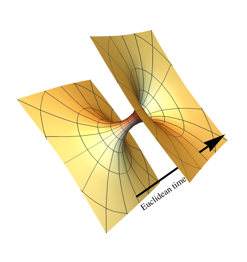
Figure 1: The Euclidean wormhole solution connects two asymptotically flat regions (left panel). The minimum size of the wormhole throat defines the characteristic length $L$ in eq. (17). The wormhole throat is characterized by the axion charge $n$ (see eq. (18)). This characteristic allows for the possibility to interpret the wormhole as the combination of an instanton with axion charge $+n$ and an anti-instanton with axion charge $-n$ (right panel).

The flipped sign in eqs. (8,11) plays a crucial rôle in what follows. The mere existence of wormhole solutions – as we shall see – is a peculiar property of massless free pseudo-scalar (scalar) fields, which admit a dual description in terms of a two-index antisymmetric tensor (pseudo-tensor) whose field strength is the three-form $H$ in eq. (5). Indeed, even if we focus on the case of a pseudo-scalar axion field, it is important to remark that the construction we put forward in this section remains valid also for a genuine scalar field.

We now look for a spherically symmetric solution with the following ansatz

$$ds^{2}=\alpha^{2}(r)dr^{2}+\beta^{2}(r)d\Omega^{2}_{D-1,\mathcal{K}}~{},~{}~{}~{}~{}~{}~{}H_{\mu\nu\rho}=\mathcal{H}(r)\epsilon_{ijk}~{},$$ (12)

where $r$ is the time coordinate in Euclidean space, and the $D-1$ space has curvature $\mathcal{K}$. Without loss of generality, we write $d\Omega^{2}_{D-1,\mathcal{K}}=\hat{g}_{ij}d\varphi^{i}d\varphi^{j}$, with metric determinant $\sqrt{g}=\alpha\beta^{3}\sqrt{\hat{g}}$. $\mathcal{K}=1$ corresponds to a closed geometry, and for $D=4$ $d\Omega^{2}_{D-1,\mathcal{K}=1}$ reduces to the ordinary three-sphere whose metric can be parametrized in terms of three angles as $d\Omega^{2}_{3,1}=(d\psi^{2},\sin^{2}\psi d\phi^{2},\sin^{2}\psi\sin^{2}\phi d\varphi^{2})$. On the contrary, $\mathcal{K}=-1$ describes an open geometry, with $d\Omega^{2}_{3,-1}=(d\psi^{2},\sinh^{2}\psi d\phi^{2},\sinh^{2}\psi\sin^{2}\phi d\varphi^{2})$. In eq. (12) the indices in $\epsilon_{ijk}$ run over the three-dimensional space $d\Omega^{2}_{3,\mathcal{K}}$, and they are raised and lowered by the induced metric $\hat{g}$.

The scalar curvature is

$$\mathcal{R}=\frac{6\left\{\mathcal{K}\alpha^{3}+\beta\beta^{\prime}\alpha^{\prime}-\alpha\left[(\beta^{\prime})^{2}+\beta\beta^{\prime\prime}\right]\right\}}{\alpha^{3}\beta^{2}}~{},$$ (13)

and the Einstein equations are

$$G_{rr}=-\frac{3\mathcal{K}\alpha^{2}}{\beta^{2}}+\frac{3(\beta^{\prime})^{2}}{\beta^{2}} = \frac{8\pi}{M_{\rm Pl}^{2}}\left(-3\mathcal{F}\alpha^{2}\mathcal{H}^{2}\right)~{},$$ (14)

$$G_{ij}=\hat{g}_{ij}\left[-\mathcal{K}-\frac{2\beta\beta^{\prime}\alpha^{\prime}}{\alpha^{3}}+\frac{(\beta^{\prime})^{2}}{\alpha^{2}}+\frac{2\beta\beta^{\prime\prime}}{\alpha^{2}}\right] = \hat{g}_{ij}\frac{8\pi}{M_{\rm Pl}^{2}}\left(3\mathcal{F}\beta^{2}\mathcal{H}^{2}\right)~{}.$$ (15)

Notice that the field ansatz in eq. (12) automatically solves the equation of motion $\partial_{\mu}\left(\sqrt{g}H_{\alpha\nu\rho}g^{\alpha\mu}\right)=0$. On the contrary, the Bianchi identity $\epsilon^{\mu\nu\rho\sigma}(\partial_{\rho}H_{\sigma\mu\nu})=0$ provides a non-trivial constraint. Using the field ansatz, and bearing in mind that $\epsilon_{ijk}=\beta^{3}\sqrt{\hat{g}}\varepsilon_{ijk}$ (see footnote $2$), we find $\partial_{r}(H\epsilon_{ijk})$ = $\partial_{r}(\mathcal{H}\beta^{3}\sqrt{\hat{g}}\varepsilon_{ijk})$ = 0. As a direct consequence, we have the $r$ dependence $\mathcal{H}(r)=\mathcal{H}_{0}/\beta^{3}(r)$, with $\mathcal{H}_{0}$ dimensionless constant. To make contact with the original solution proposed in [16], we now restrict the analysis to the three-sphere $S_{3}$, with $\mathcal{K}=1$ and $\beta^{2}(r)=r^{2}$. The constant $\mathcal{H}_{0}$ can be fixed by normalizing the integral of the field strength over $S_{3}$. We have

$$\int_{S_{3}}\mathcal{H}_{0}\,d\Omega_{3,1}=2\pi^{2}\mathcal{H}_{0}=n~{},$$ (16)

where - as we shall see later - $n$ is an integer number. We can now use eq. (14). Solving for $\alpha$, we find

$$\alpha^{2}(r)=\frac{1}{1-L^{4}/r^{4}}~{},~{}~{}~{}~{}~{}~{}~{}L\equiv\left(\frac{n^{2}}{3\pi^{3}M_{\rm Pl}^{2}f_{a}^{2}}\right)^{1/4}~{}.$$ (17)

The metric in eqs. (12,17) describes the Giddings-Strominger wormhole configuration. The wormhole connects two asymptotically flat Euclidean region, as shown in the left panel of fig. 1. At any fixed Euclidean time $r$, the cross-section of the wormhole is a three-sphere. The length scale $L$ in eq. (17) defines the minimal radius of the wormhole throat. Let us note that there is no singularity at $L=0$; this is indeed nothing but a coordinate singularity, as we shall discuss later.

Using the relation $H_{\mu\nu\rho}=f_{a}^{2}\epsilon_{\mu\nu\rho\sigma}(\partial^{\sigma}\theta)=\epsilon_{\mu\nu\rho\sigma}J^{\sigma}$ and the field ansatz in eq. (12) we can compute the axion charge stored in a cross-section of the wormhole throat. We find

$$\mathcal{Q}\equiv\int_{S^{3}}f_{a}^{2}\left(\partial^{r}\theta\right)\beta^{3}(r)d\Omega_{3,1}=\int_{S_{3}}\mathcal{H}_{0}\,d\Omega_{3,1}=2\pi^{2}\mathcal{H}_{0}=n~{}.$$ (18)

The wormhole throat is therefore characterized by the axion charge $n$. This characteristic offers the possibility to consider the wormhole as the combination of an instanton with axion charge $+n$ and an anti-instanton with axion charge $-n$ (fig. 1, right panel). Furthermore, as we shall discuss at the end of this section, $n$ is quantized, and it only takes integer values. As discussed in [16], separating the wormhole in two halves has an important topological interpretation. On the one hand, the wormhole interpolates between two $\mathbb{R}^{3}$ geometries widely separated in time. On the other one, the instanton (anti-instanton) represents a topology change from $\mathbb{R}^{3}$ to $\mathbb{R}^{3}\oplus S_{3}$ (from $\mathbb{R}^{3}\oplus S_{3}$ to $\mathbb{R}^{3}$).

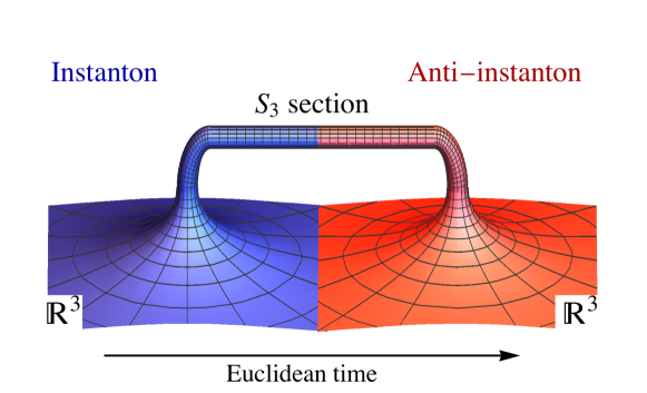
Figure 2: Pictorial representation of an euclidean wormhole with endpoints connected to the same asymptotically flat space. The Euclidean time runs in the direction of the arrow. At each instant of time, two space dimensions have been suppressed. The cross-section of the wormhole throat is a three-sphere $S_{3}$.

Instead of considering the wormhole as connecting two separate asymptotic Euclidean spaces - a configuration that has an unclear physical interpretation - it is possible to consider wormholes that connect back to the same space, as shown in fig. 2. By slicing the wormhole in half, the instanton/anti-instanton represents, as before, a topology change from $\mathbb{R}^{3}$ to $\mathbb{R}^{3}\oplus S_{3}$ and viceversa.

From eq. (5), we can compute the action of an instanton configuration with charge $n$. Using $\mathcal{R}=-8\pi G_{N}\mathcal{F}H^{2}$, we find

$$\mathcal{S}_{\rm inst}=\int d^{4}x\sqrt{g}\mathcal{F}H^{2}=\frac{n^{2}}{4\pi^{4}f_{a}^{2}}\int_{L}^{\infty}dr\int d\Omega_{3,1}\frac{1}{r^{3}\sqrt{1-\frac{L^{4}}{r^{4}}}}=\frac{\sqrt{3\pi}nM_{\rm Pl}}{8f_{a}}=\frac{3\pi^{2}M_{\rm Pl}^{2}L^{2}}{8}~{}.$$ (19)

This is the right moment to do some useful dimensional analysis, and it is convenient to restore the appropriate powers of $\hbar$ (while keeping $c=1$). Equivalently, we can introduce a unit of energy $\mathrm{E}$ and length $\mathrm{L}$, with $[\hbar]=\mathrm{E\,L}$. Natural units correspond to $\mathrm{E}=\mathrm{L}^{-1}$. It is straightforward to realize – using the fact that a generic Lagrangian density has dimension $[\mathcal{L}]=\mathrm{E}\,\mathrm{L}^{-3}$ – that the canonically normalized axion field has dimension $[a]=\mathrm{E}^{1/2}\mathrm{L}^{-1/2}$. Similarly, the dimension of a coupling constant (like a gauge coupling) is $[\mathrm{g}]=\mathrm{E}^{-1/2}\mathrm{L}^{-1/2}$. The axion decay constant $f_{a}$ is a VEV, and it shares the same dimensionality of the electroweak VEV and the Planck scale: $[f_{a}]=[v]=[M_{\rm Pl}]=\mathrm{E}^{1/2}\mathrm{L}^{-1/2}$. From eq. (18) the dimensionality of the axion charge is $[n]=\mathrm{E}\,\mathrm{L}$, and it corresponds to an inverse coupling squared. Finally, from eq. (17) we see that $L$ is a genuine length scale. From this simple analysis we learn a number of interesting things.

First, we can exploit the analogy with the electroweak theory. The Fermi constant $G_{F}$ (or equivalently the electroweak VEV) is related to the ratio between the electroweak mass (defined here by the mass of the $W$ boson, and corresponding to the physical threshold of energy $\mathrm{E}\sim M_{W}$ at which the new degrees of freedom in the electroweak sector become dynamical) and the electroweak coupling constant $\mathrm{g}_{W}$ by means of $[v]=[G_{F}]^{-1/2}=[M_{W}]/[\mathrm{g}_{W}]$. Similarly, in gravity we expect the relation

$$[M_{\rm Pl}]=[G_{N}]^{-1/2}=\frac{[M_{S}]}{[\mathrm{g}_{S}]}~{},$$ (20)

where we introduced a string mass scale $M_{S}$ and a string coupling $\mathrm{g}_{S}$. If the UV completion of general relativity is weakly coupled, we expect new degrees of freedom to occur even below the Planck scale. If, on the contrary, the UV completion of general relativity is strongly coupled, $\mathrm{g}_{S}\gtrsim 1$, we expect the new dynamics of quantum gravity to occur above $M_{\rm Pl}$. We shall return on this point later, discussing the validity of the wormhole solutions (see section 6.2).

Second, from eq. (19) we recover the correct dimensionality of an instanton action since we have that $[\mathcal{S}_{\rm inst}]=1/[\mathrm{g}]^{2}=[\hbar]$. On general ground, this also explains why instantons are non-perturbative. If $\mathrm{g}\to 0$, $\exp(-\mathcal{S}_{\rm inst}/\hbar)$ goes to zero faster then any power of $\mathrm{g}$, and instanton effects cannot be captured at any finite order in perturbation theory.

Finally, notice that the wormholes with action given in eq. (19) realize the Weak Gravity Conjecture (WGC) proposed in [21]. The generalization of the WGC to the case of axions states that for an axion with decay constant $f_{a}$ there exists an instanton with action $\mathcal{S}_{\rm inst}\lesssim M_{\rm Pl}/f_{a}$. In the context of Einstein gravity, this is precisely the wormhole with $n=1$ and $\mathcal{S}_{\rm inst}\simeq 0.38\,M_{\rm Pl}/f_{a}$.

Let us now explore in more detail our solution. The wormhole metric

$$ds^{2}=\left(\frac{1}{1-L^{4}/r^{4}}\right)dr^{2}+r^{2}d\Omega_{3,1}$$ (21)

is conformally equivalent to a flat metric on $S_{3}\times\mathbb{R}$. The coordinate transformation

$$\left(\frac{d\tau}{dr}\right)^{2}=\frac{r^{2}}{r^{4}-L^{4}}~{}~{}~{}~{}~{}~{}\Longrightarrow~{}~{}~{}~{}~{}~{}\tau(r)=\frac{1}{2}\ln\left[\frac{r^{2}+\sqrt{r^{4}-L^{4}}}{L^{2}}\right]~{},$$ (22)

brings the metric in eq. (21) into the form

$$ds^{2}=a^{2}(\tau)\left(d\tau^{2}+d\Omega_{3,1}\right)~{},~{}~{}~{}~{}a^{2}(\tau)=L^{2}\cosh(2\tau)~{}.$$ (23)

Notice that $r=L$ is mapped to $\tau=0$ and in this coordinate system is plain to see that there is no singularity and the wormhole connects the two asymptotically flat regions at $\tau=\pm\infty$. With respect to this metric, the Einstein equations and the equation of motion for the axion field, which can be obtained from taking $\alpha=\beta=a$ in eqs. (14,15), are

$$-3+3\left(\frac{a^{\prime}}{a}\right)^{2}=-\frac{f_{a}^{2}\kappa}{2}(\theta^{\prime})^{2}~{},~{}~{}~{}~{}2\frac{a^{\prime\prime}}{a}-\left(\frac{a^{\prime}}{a}\right)^{2}-1=\frac{f_{a}^{2}\kappa}{2}(\theta^{\prime})^{2}~{},~{}~{}~{}~{}\theta^{\prime\prime}+(2a^{\prime}/a)\theta^{\prime}=0~{},$$ (24)

where we defined $\kappa\equiv 8\pi/M_{\rm Pl}^{2}$. From the first Einstein equation, we find

$$f_{a}^{2}\kappa(\theta^{\prime})^{2}=\frac{6}{\cosh^{2}(2\tau)}~{}.$$ (25)

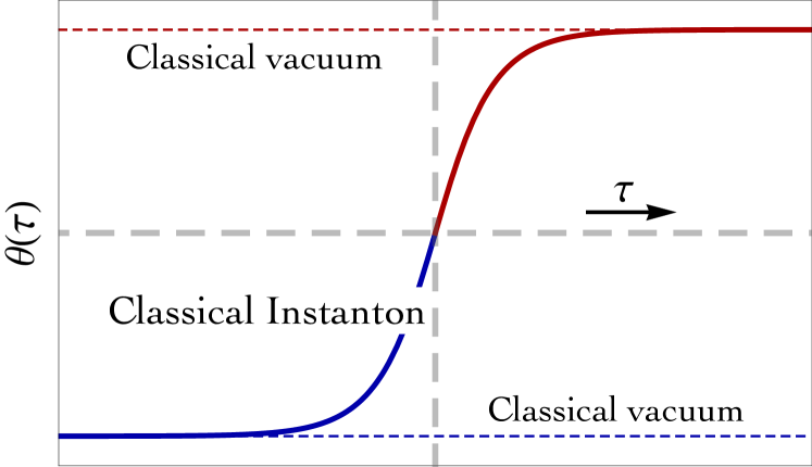
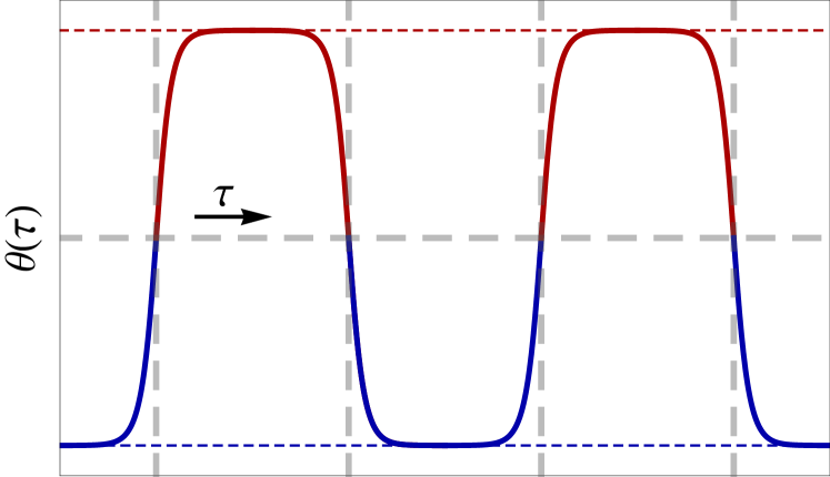
Figure 3: Axion field profile corresponding to the wormhole solution in eq. (26). The blue and red colors describe the instanton and anti-instanton part of the solution (see fig. 1). A string of widely separated instantons and anti-instantons (right panel) provides an approximate stationary point of the Euclidean action (which becomes an exact solution of the equation of motion only asymptotically, in the limit of infinite separation).

Integrating over $\tau$, we find

$$f_{a}^{2}\kappa\theta(\tau)=\sqrt{6}\arctan\left[\tanh(\tau)\right]~{}.$$ (26)

In the left panel of fig. 3 we show the instanton solution in eq. (26). Asymptotically, the axion field configuration approaches the constant values $f_{a}^{2}\kappa\theta(\tau)/\sqrt{6}\overset{\tau\to\pm\infty}{\rightarrow}\pm\pi/4$, and features a sharp transition in between. Notice that the asymptotic limit is exponentially fast, $\tanh(\tau)\overset{\tau\to\pm\infty}{\rightarrow}\pm\left(1-e^{-2\tau}\right)$. Since instantons are well-localized objects, there are also approximate solutions consisting of strings of widely separated instantons and anti-instantons centered at $\tau_{1},\dots,\tau_{m}$. Notice that the possibility to center the instanton-anti-instanton pair at an arbitrary position in $\tau$ is due to the fact that the wormhole solution in eqs. (23,25) possesses a ‘time’-translation symmetry. Indeed, the most general solution of the field equations is $a^{2}(\tau)=L^{2}\cosh[2(\tau-\tau_{0})]$, $f_{a}^{2}\kappa(\theta^{\prime})^{2}=6/\cosh^{2}[2(\tau-\tau_{0})]$, and it depends on the arbitrary constant $\tau_{0}$. As we shall see in section 3.1, the presence of this ‘time’-translation symmetry will imply the existence of a zero eigenvalue in the spectrum of the quadratic action describing fluctuations around the wormhole solution. For illustrative purposes, we show a multi-instanton solution in the right panel of fig. 3. Since the $m$ instantons are widely separated, the classical action is just $m\mathcal{S}_{\rm inst}$.

Finally, we close this section with the following remark. As already anticipated, the axion charge in eq. (18) turns out to be quantized. This property can be understood as follows. We consider the action for the axion field in the background metric of eq. (23), and, after introducing the new variable $d\tau/d\sigma\equiv a^{2}$ and considering radially symmetric field configurations $\theta(\tau(\sigma))$, we find

$$\mathcal{S}_{\theta}=2\pi^{2}\int d\sigma\frac{f_{a}^{2}}{2}\left(\frac{d\theta}{d\sigma}\right)^{2}~{}.$$ (27)

With respect to the new variable, the equation of motion of the axion field is simply given by $d^{2}\theta/d\sigma^{2}=0$. Equivalently, using eqs. (23,25), we find $d\theta/d\sigma={\rm const}=n/2\pi^{2}f_{a}^{2}$. We can now expand eq. (27) around the instanton solution, $\theta\to\theta+\delta\theta$. We find, using the equation of motion, the following change in the action

$$\delta\mathcal{S}_{\theta}=2\pi^{2}f_{a}^{2}\int d\sigma\frac{d}{d\sigma}\left(\delta\theta\frac{d\theta}{d\sigma}\right)=2\pi^{2}f_{a}^{2}\delta\theta\left.\frac{d\theta}{d\sigma}\right|_{\rm boundary}=n\delta\theta~{}.$$ (28)

In the presence of wormholes, the action is no longer invariant under the generic shift $\theta\to\theta+\delta\theta$. We now restrict to the discrete transformations $\delta\theta=2k\pi$, with $k\in\mathbb{Z}$. Since $\theta$ is an angular variable, we know that $\theta\to\theta+2k\pi$ corresponds to the same physical point, as discussed in section 1. This is a gauge redundancy, and, as such, it cannot be broken. The simple observation is that quantum mechanical transition amplitudes involve $e^{\imath\mathcal{S}_{\theta}}$, and the phase exponential must be gauge invariant. This means that the only change $\delta\mathcal{S}_{\theta}$ that can be tolerated corresponds to an integer multiple of $2\pi$. We therefore find the quantization condition $n\in\mathbb{Z}$.

The quantization of the wormhole charge $\mathcal{Q}$ – and the subsequent invariance of the action under the transformation $\theta\to\theta+2k\pi$, with $k\in\mathbb{Z}$ – is a crucial point, since it is related to the fact that in the presence of wormholes the continuos shift symmetry in eq. (1) is broken down to its discrete subgroup in eq. (2). We shall elaborate more on this point in section 4.

The quantization of the wormhole charge $\mathcal{Q}$ is tightly related to the periodicity of the axion field, and it has a profound mathematical explanation. It is indeed possible to show that $n$ can only be either an integer or zero. The point is that if the flux of the three-form $H$ through $S_{3}$ is non-zero, then in general a unique two-form potential $B$ – an antisymmetric tensor whose filed strength is $H$ according to $H_{\mu\nu\rho}=\partial_{\mu}B_{\nu\rho}+\partial_{\nu}B_{\rho\mu}+\partial_{\rho}B_{\mu\nu}$, see appendix A – covering the whole sphere $S_{3}$ does not exist. Only if $n$ is an integer the ambiguity can be bypassed by defining two potentials $B_{1,2}$, covering the upper and lower halves of $S_{3}$, and related to each other by a gauge transformation in an overlap region which is topologically $S_{2}$ [24, 25, 26]. The argument is very similar to the Dirac quantization of the electric charge in the presence of a magnetic monopole. We discuss in more detail this point in appendix A.3. The analogy is indeed deeper, and the Dirac quantization condition corresponds to the quantization of the axion charge over a spatial slice $S_{3}$ [27, 28].

2.2 The Gibbons-Hawking-York boundary term

In the presence of a manifold with boundary, the Einstein-Hilbert action in eq. (5) must be supplemented by a boundary term so that the variational principle is well-defined [29, 30, 31]. To make this point clear, let us only focus on the term involving the Ricci scalar for the metric ansatz in eq. (23) with $\mathcal{R}=6(a-a^{\prime\prime})/a^{3}$

$$\mathcal{S}=-\frac{3M_{\rm Pl}^{2}}{8\pi}\int d\Omega_{3,1}d\tau\left(a^{2}-aa^{\prime\prime}\right)\\ =-\frac{3M_{\rm Pl}^{2}}{8\pi}\int d\Omega_{3,1}d\tau\left[a^{2}+(a^{\prime})^{2}-\frac{d(aa^{\prime})}{d\tau}\right]~{}.$$ (29)

The presence of the second derivative prevents the correct formulation of the variational principle. It is therefore necessary to add the Gibbons-Hawking-York boundary term, whose general form is given by

$$\mathcal{S}_{\rm GHY}=-\frac{M_{\rm Pl}^{2}}{8\pi}\int_{\partial M}d^{3}\vec{x}\sqrt{h}\left(K-K_{0}\right)~{},$$ (32)

where $h$ is the determinant of the induced metric on the boundary manifold $\partial M$, $K$ is the trace of the extrinsic curvature tensor, and $K_{0}$ is the trace of the extrinsic curvature tensor of the same boundary embedded in flat spacetime. The explicit computation of $\mathcal{S}_{\rm GHY}$ is straightforward. The trace of the extrinsic curvature tensor is $K=\nabla_{\mu}n^{\mu}=\partial_{\mu}n^{\mu}+\Gamma^{\mu}_{\mu\nu}n^{\nu}$, where $n^{\mu}$ is the unit normal to $\partial M$. The boundary we are interested in are hypersurfaces of constant $\tau$, and the corresponding unit normal vector is $n^{\tau}=1/a$. By direct computation, we find $K=3a^{\prime}/a^{2}$. As far as $K_{0}$ is concerned, we use $a=e^{\tau}$ for the flat metric, and we find $K_{0}=3/a$. All in all, the Gibbons-Hawking-York boundary term reduces to

$$\mathcal{S}_{\rm GHY}=-\frac{3M_{\rm Pl}^{2}}{8\pi}\int d\Omega_{3,1}\left(aa^{\prime}-a^{2}\right)~{},$$ (33)

and it cancels the total derivative in eq. (29).

The Gibbons-Hawking-York boundary term must be included for a correct formulation of the gravitational action in the presence of a manifold with boundary, and this is the case for the half-wormhole configuration. It is therefore important to evaluate the topological contribution of eq. (33) to the bulk action in eq. (19). Using the explicit solution in eq. (23), we find

$$\mathcal{S}_{\rm GHY}=-\frac{3M_{\rm Pl}^{2}\pi}{4}\left|aa^{\prime}-a^{2}\right|_{\tau=0}^{\tau=\infty}=-\frac{3M_{\rm Pl}^{2}\pi L^{2}}{4}=-\left(\frac{2}{\pi}\right)\frac{\sqrt{3\pi}nM_{\rm Pl}}{8f_{a}}~{},$$ (34)

where only the boundary at the wormhole throat gives a non-vanishing contribution. Taking into account the boundary term, the action of an instanton configuration with charge $n$ is

3 Quadratic action and the absence of negative modes

Instantons are responsible for one of the most important effect in Quantum Mechanics, that is the tunneling through a potential barrier.

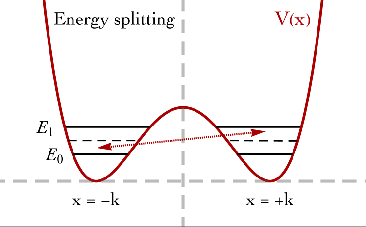
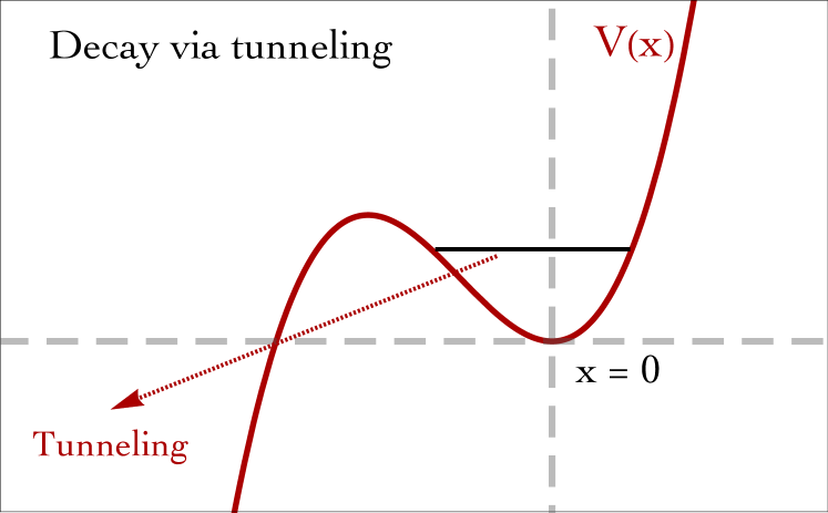
Figure 4: Tunneling through a potential barrier in Quantum Mechanics mediated by non-perturbative instanton solutions.

The importance of such effect lies in the fact that it changes the vacuum of the system, and there exist two paradigmatic situations in which this effect is particularly manifest [22, 23].

In the left panel of fig. 4 we show a one-dimensional quantum system featuring a potential with a double well, of the form $V(x)=\lambda(x^{2}-k^{2})^{2}$. In perturbation theory, the ground state has two degenerate minima at $x=\pm k$, which are equivalent because of the reflection symmetry of the system (dashed black lines). Instantons lift the degeneracy, and the energy difference between the true ground state and the first excited state (solid black lines – respectively, the anti-symmetric and symmetric combination of the two vacua at $x=\pm k$) is controlled by the instanton action, according to the qualitative scaling $E_{1}(\mathrm{g})-E_{0}(\mathrm{g})\sim e^{-{\rm const}/\mathrm{g}^{2}}$.

In the right panel of fig. 4 we show a potential with a metastable vacuum, of the form $V(x)=m\omega^{2}x^{2}+\lambda x^{3}$. In perturbation theory – assuming small $\lambda$ – one can compute the energy of the ground state of the system at, in principle, any order (solid black line). However, perturbation theory can not describe the tunneling through the barrier, and the instability of the vacuum. Again, the tunneling is captured by instanton effects, that in this case introduce a small imaginary part in the ground state energy, $E_{0}(\mathrm{g})={\rm Re\,}E_{0}(\mathrm{g})+\imath{\rm Im\,}E_{0}(\mathrm{g})$, with ${\rm Im\,}E_{0}(\mathrm{g})\sim e^{-{\rm const}/\mathrm{g}^{2}}$, which in turn becomes a decay probability in the time evolution $e^{\imath E_{0}(\mathrm{g})t}$. In this case the instanton is called bounce.

In order to understand the true nature of the instanton, it is necessary to inspect the action at the quadratic order. Let us clarify this point with an explicit example. In Euclidean time, the quantum probability amplitude from the initial state $|i\rangle$ at time $-T/2$ to the final state $|f\rangle$ at time $T/2$ – that corresponds, for instance, to the transition amplitude between the two vacua in the quantum systems discussed in fig. 4 – is given by

$$\langle f|e^{-TH}|i\rangle=\sum_{n}e^{-TE_{n}}\langle f|n\rangle\langle n|i\rangle\approx\frac{\mathcal{N}}{\sqrt{{\rm det}^{\prime}\left(\frac{\delta^{2}\mathcal{S}_{\rm E}}{\delta x^{2}}\right)}}e^{-\mathcal{S}_{\rm E}[x_{\rm cl}(\tau)]}~{}.$$ (36)

where $\mathcal{N}$ is a normalization constant, $\mathcal{S}_{\rm E}[x_{\rm cl}(\tau)]$ is the Euclidean action computed for the classical instanton solution $x_{\rm cl}(\tau)$, and the prefactor encodes the quantum fluctuation around the classical trajectory. The latter, as a result of a Gaussian integration, takes the shape of a determinant with a prime denoting the subtraction of zero eigenvalues. If we take $T$ to be very large, the lowest energy state dominates the sum, and we can extract the ground state energy from the computation of the path integral. The spectrum of the differential operator $\delta^{2}\mathcal{S}_{\rm E}/\delta x^{2}$ is therefore crucial. In the presence of one (or an odd number of) negative eigenvalue(s), there is an imaginary contribution to the vacuum energy, and the instanton plays the rôle of a bounce. If the spectrum of the quadratic action is positive (or if the number of negative eigenvalues is even) the vacuum energy is real, and the instanton describes the transition between degenerate vacua, lifting their degeneracy as discussed in the case of the double well.

The analogy with one-dimensional systems in Quantum Mechanics suits particularly well our case since the wormhole solutions discussed in section 2 are characterized by one relevant dimension, that is the time coordinate in the Euclidean 4D space.

3.1 Bulk action and boundary terms

In this section we study, motivated by the previous discussion, the spectrum of the quadratic action describing perturbations around the Euclidean wormhole solution. To this end, we shall exploit the formalism developed in the context of cosmological perturbation theory for the analysis of fluctuations of a scalar field $\varphi_{0}$ coupled to gravity in a Friedmann-Robertson-Walker metric [32]. This study requires the canonical formalism in order to correctly get rid of the non-dynamical degrees of freedom, as in any other gauge theory. The canonical formulation, although non-explicitly, preserves gauge invariance.

In the following, we start considering metric perturbations in Minkowski space around the background line element $ds^{2}=a^{2}(\eta)(-d\eta^{2}+\gamma_{ij}dx^{i}dx^{j})$. Including fluctuations, in full generality we write $ds^{2}=a^{2}(\eta)\left[-(1+2A)d\eta^{2}+2B_{i}dx^{i}d\eta+(\gamma_{ij}+h_{ij})dx^{i}dx^{j}\right]$. This perturbed line element can be further analyzed by means of the scalar-vector-tensor decomposition, which separates the fluctuations into components according to their transformations under spatial rotations. In particular, the three-vector $B_{i}$ splits into the gradient of a scalar, and a divergence-free vector $B_{i}=\partial_{i}B+\hat{B}_{i}$ while the symmetric tensor $h_{ij}$ can be decomposed into a scalar part, a divergence-free vector, and a trace-free transverse tensor $h_{ij}=-2\psi\gamma_{ij}+2\partial_{\langle i}\partial_{j\rangle}E+2\partial_{(i}\hat{E}_{j)}+t_{ij}$. The advantage of this decomposition is that scalar, vector and tensor Einstein equations are decoupled at the linear order and can therefore be treated separately. Vector perturbations are pure gauge modes, and they carry no dynamics [32]. As far as tensor perturbations are concerned, they do not couple to scalar modes, and we can therefore rely on standard computations of gravitational waves in instanton background [33]. We found a positive spectrum, and we summarize our computation in appendix C.

We focus here on scalar perturbations. The perturbed line element is therefore

$$ds^{2}=a^{2}(\eta)\left\{-(1+A)d\eta^{2}+2\partial_{i}Bdx^{i}d\eta+[\gamma_{ij}(1-2\psi)+2\partial_{\langle i}\partial_{j\rangle}E]dx^{i}dx^{j}\right\}~{},$$ (37)

where we simultaneously expand the scalar field, assumed to be function of $\eta$, as $\varphi_{0}+\delta\varphi$.

The second order Lagrangian in terms of the perturbations in eq. (37) can be found in e.g. [32], but it has, at this level, non-dynamical degrees of freedom and gauge redundancy. First $A$ and $B$ are not dynamical, that is they do not have a ‘kinetic term’; they behave like $A_{0}$ in a ‘conventional’ gauge theory. In addition, there is a two-parameter gauge transformation, corresponding to diffeomorphism acting on scalar perturbations, given by $\delta x^{\mu}=(\lambda^{0},\partial^{i}\lambda)$, and we have

$$\delta\psi=-\frac{\dot{a}}{a}\lambda^{0}~{},~{}~{}~{}~{}~{}~{}~{}\delta B=\dot{\lambda}-\lambda^{0}~{},~{}~{}~{}~{}~{}~{}~{}\delta E=\lambda~{},~{}~{}~{}~{}~{}~{}~{}\delta(\delta\varphi)=\dot{\varphi}_{0}\lambda^{0}~{},$$ (38)

where we indicate with $\dot{}$ the derivative w.r.t. the time variable $\eta$. Out of the 5 perturbations $A,B,E,\psi,\delta\varphi$, 2 are non dynamical, and 2 can be removed via a gauge transformation which leaves us with 1 d.o.f. All in all, we have the following quadratic action in Hamiltonian form $p\dot{q}-\mathscr{H}$ (see [32] for details of the derivation)

$$\delta\mathcal{S}^{(2)}=$$ (39)

$$\int d\eta d\vec{x}\left\{\Pi_{\Psi}\dot{\Psi}-\frac{2a^{2}\sqrt{\gamma}}{\kappa^{2}\dot{\varphi}_{0}^{2}}\left[\left(\Delta+3\mathcal{K}\right)\Psi+\frac{\kappa\dot{a}/a}{2a^{2}\sqrt{\gamma}\Pi_{\Psi}}\right]^{2}-\frac{a^{2}\sqrt{\gamma}}{\kappa}\Psi\left(\Delta+3\mathcal{K}\right)\Psi+\frac{1}{4a^{2}\sqrt{\gamma}}\Pi_{\Psi}\frac{\kappa\mathcal{K}}{(\Delta+3\mathcal{K})}\Pi_{\Psi}\right\}~{},$$

where the dynamical variable $\Psi$ and its conjugate momentum $\Pi_{\Psi}$ in terms of the metric perturbations in eq. (37) are $\Psi\equiv\psi+(\dot{a}/a)\delta\varphi/\dot{\varphi}_{0}$ and $\Pi_{\Psi}\equiv\Pi_{\psi}-2a^{2}\sqrt{\gamma}(\Delta+3\mathcal{K})\delta\varphi/\kappa\dot{\varphi}_{0}$, where $\Pi_{\psi}$ is the conjugate momentum of $\psi$ and $\Delta$ is the Laplacian on the three-sphere associated with $\gamma_{ij}$. The background solutions satisfy

$$\left(\frac{\dot{a}}{a}\right)^{2}+\mathcal{K}-\frac{\kappa}{6}\dot{\varphi}_{0}^{2}=0~{},~{}~{}~{}~{}~{}~{}~{}~{}~{}~{}~{}~{}~{}\ddot{\varphi}_{0}+2\frac{\dot{a}\dot{\varphi}_{0}}{a}=0~{}.$$ (40)

In the following we focus on the spatially homogeneous $O(4)$ invariant modes, and we formally set $\Delta=0$. As discussed in [34, 35], the homogeneous modes are those that are potentially responsible for the presence of negative eigenvalues in the spectrum of the quadratic action, and they need to be carefully analyzed. Indeed, in [36] the authors claimed the existence of a negative mode among the homogenous fluctuations around the Giddings-Strominger wormholes. If true, this result would imply that wormholes are bounce solutions mediating unstable vacuum decay via tunneling transition. Motivated by the necessity to further explore and check this result, we now turn to discuss our own analysis. For completeness, in appendix C we discuss the spectrum of inhomogeneous scalar perturbations.

Restricting to the homogeneous modes, eq. (39) becomes

$$\left.\delta\mathcal{S}^{(2)}\right|_{\Delta=0}=\int d\eta d^{3}\vec{x}\left[\Pi_{\Psi}\dot{\Psi}-\left(\begin{array}[]{cc}\Psi&\Pi_{\Psi}\end{array}\right)\left(\begin{array}[]{cc}\frac{3\mathcal{K}a^{2}\sqrt{\gamma}(6\mathcal{K}+\kappa\dot{\varphi}_{0}^{2})}{\kappa\dot{\varphi}_{0}^{2}}&\frac{3\mathcal{K}\dot{a}}{\kappa a\dot{\varphi}_{0}^{2}}\\ \frac{3\mathcal{K}\dot{a}}{\kappa a\dot{\varphi}_{0}^{2}}&\frac{6\dot{a}^{2}-\kappa a^{2}\dot{\varphi}_{0}^{2}}{12a^{4}\sqrt{\gamma}\dot{\varphi}_{0}^{2}}\end{array}\right)\left(\begin{array}[]{c}\Psi\\ \Pi_{\Psi}\end{array}\right)\right]~{}.$$ (41)

The first difficulty one faces is the conformal factor problem [37]. The conformal factor problem can be spotted in the Hamiltonian of eq. (41) by using the equation of motion $6\dot{a}^{2}-\kappa a^{2}\dot{\varphi}_{0}^{2}=-6\mathcal{K}a^{2}$. As a consequence, we find a ‘wrong sign’ kinetic term since we will be looking at the closed case $\mathcal{K}=1$. The literature often treats this problem by just turning $\Psi$ into the imaginary axis but this, other than pretty arbitrary, will lead to augmented confusion when convoluted with the rotation to Euclidean. Instead the most sensible way in our humble opinion is to perform a canonical (symplectic) transformation and study the resulting system as done in [34]. This will correspond roughly to swapping $\Psi$ and $\Pi_{\Psi}$ and then performing another transformation, explicitly and in a single step

$$\Pi_{\Psi}=-\frac{3a^{2}\sqrt{\gamma}}{\dot{\varphi}_{0}}q-\frac{\dot{\varphi}_{0}\dot{a}}{\kappa a}p~{},~{}~{}~{}~{}~{}~{}~{}~{}~{}\Psi=-\frac{\kappa a}{2\dot{\varphi}_{0}\dot{a}}q+\frac{\dot{\varphi}_{0}}{6a^{2}\sqrt{\gamma}}p~{},$$ (45)

which is symplectic since

$$J^{\rm T}\left(\begin{array}[]{cc}0&1\\ -1&0\end{array}\right)J=\left(\begin{array}[]{cc}0&1\\ -1&0\end{array}\right)~{}~{}~{}~{}~{}~{}{\rm with}~{}~{}~{}~{}~{}\left(\begin{array}[]{c}\Psi\\ \Pi_{\Psi}\end{array}\right)=J\left(\begin{array}[]{c}p\\ q\end{array}\right)~{}.$$ (46)

and leads to the action

$$\left.\delta\mathcal{S}^{(2)}\right|_{\Delta=0}=\int d\eta d^{3}\vec{x}\left[p\dot{q}-\left(\begin{array}[]{cc}q&p\end{array}\right)\left(\begin{array}[]{cc}0&\frac{3\mathcal{K}-\kappa\dot{\varphi}_{0}^{2}}{3\dot{a}/a}\\ \frac{3\mathcal{K}-\kappa\dot{\varphi}_{0}^{2}}{3\dot{a}/a}&\frac{2\mathcal{K}^{2}}{\kappa^{2}a^{2}\sqrt{\gamma}}\end{array}\right)\left(\begin{array}[]{c}q\\ p\end{array}\right)\right]~{},$$ (47)

where we discarded boundary terms since the equation above is the starting point for a canonical formulation, as discussed in sec. 2.2 and in accordance with [35].

The canonical transformation above might appear to have no other virtue than to simplify the Hamiltonian, so it is worth pausing and looking at its connection with the original variables and physical interpretation. Indeed in ref. [32] a similar canonical transformation is used such that the resulting coordinate is proportional to Bardeen’s potential. In our case we have, after substituting in the canonical transformation:

$$q=\frac{1}{\kappa}\left\{\dot{\varphi}_{0}\left[\mathcal{K}(B-\dot{E})-\frac{\dot{a}}{a}\psi\right]+\left(\mathcal{K}-\frac{\dot{a}^{2}}{a^{2}}\right)\delta\varphi\right\}~{},$$ (48)

which, under a gauge transformation as in eq. (38) stays invariant. The gauge invariance of the variable speaks to the success of the proccess of removing redundancies and is a valuable check on the procedure here employed.

Notice that we can write this action, since there is no ‘potential’ in the Hamiltonian for $q$, as

$$\left.\delta\mathcal{S}^{(2)}\right|_{\Delta=0}=\int d\eta d^{3}\vec{x}\frac{2\mathcal{K}^{2}}{\kappa^{2}a^{2}\sqrt{\gamma}}p^{2}~{},$$ (49)

with $p=\partial\mathscr{H}/\partial q$. It would seem that the discussion of the sign of eigenvalues ends here: they are $\geq 0$ from construction. The only non-trivial step to corroborate this conclusion is the rotation to Euclidean, which as it turns out changes nothing.

However we pursue here further to find the explicit eigenvalues of the spectrum. After using $\dot{q}=\partial\mathscr{H}/\partial p$ to write $p$ in terms of $q,\dot{q}$, repeated use of equations of motion and integration by parts leads to

$$\left.\delta\mathcal{S}^{(2)}\right|_{\Delta=0}=\int d\eta d^{3}\vec{x}\sqrt{\gamma}\left\{\frac{\kappa^{2}a^{2}}{8\mathcal{K}^{2}}\left(\dot{q}^{2}+\frac{8}{3}\kappa\dot{\varphi}_{0}^{2}q^{2}\right)-\frac{d}{d\eta}\left[\frac{\kappa^{2}a^{2}q^{2}}{4\mathcal{K}^{2}}\frac{(3\mathcal{K}-\kappa\dot{\varphi}_{0}^{2})}{\dot{a}/a}\right]\right\}~{}.$$ (50)

We note that the bulk term can be generalized to the Lorentz invariant form $d^{4}x\sqrt{-g}(\partial_{\mu}q\partial^{\mu}q+\dots)$. As the last step in Minkowski we substitute $q\to q/a$, and we find

$$\left.\delta\mathcal{S}^{(2)}\right|_{\Delta=0}=\int d\eta d^{3}\vec{x}\sqrt{\gamma}\left\{\frac{\kappa^{2}}{8\mathcal{K}^{2}}\left(-q\ddot{q}-\mathcal{K}q^{2}+\frac{5}{2}\kappa\dot{\varphi}_{0}^{2}q^{2}\right)+\frac{\kappa^{2}}{8\mathcal{K}^{2}}\frac{d}{d\eta}\left[q\dot{q}+q^{2}\left(\frac{2\kappa\dot{\varphi}_{0}^{2}-3(\dot{a}/a)^{2}-6\mathcal{K}}{3\dot{a}/a}\right)\right]\right\}~{}.$$ (51)

Finally, going to the Euclidean, $\tau=i\eta$ and with $()^{\prime}=d/d\tau$

$$\left.\delta\mathcal{S}_{\rm E}^{(2)}\right|_{\Delta=0}=\int d\tau d^{3}\vec{x}\sqrt{\gamma}\frac{\kappa^{2}}{8\mathcal{K}^{2}}\left[\left(-qq^{\prime\prime}+\mathcal{K}q^{2}-\frac{5}{2}\kappa f_{a}^{2}\theta^{\prime\,2}q^{2}\right)+\frac{d}{d\tau}\left(qq^{\prime}-\frac{2\kappa f_{a}^{2}\theta^{\prime\,2}a^{2}+3a^{\prime 2}-6a^{2}\mathcal{K}}{3aa^{\prime}}q^{2}\right)\right]~{}.$$ (52)

At this point, an important comment is in order. In addition to the usual analytical continuation, in eq. (52) we performed the formal substitution $\varphi_{0}\to\imath f_{a}\theta$. This is because the starting point of our analysis, that is the quadratic action in eq. (39), was derived in [32] considering a generic real scalar field $\varphi_{0}$. In our case, on the contrary, we are interested in the case of an axion field $\phi$ (or, more generically, in the case of a Goldstone boson which admits a three-form description). Going from Minkowski to Euclidean, in the axion case one gets an extra minus sign whenever a term quadratic in $\theta$ appears (as discussed in section 2.1 and appendix A.2), and the imaginary factor in $\varphi_{0}\to\imath f_{a}\theta$ precisely accounts for this issue. For instance, this replacement is indeed crucial to match eq. (24) starting from the corresponding Minkowski version in eq. (40).

Substituting the wormhole solution for the background fields $a$ and $\kappa f_{a}^{2}\theta^{\prime\,2}$ as given in eq. (25), and considering the case of a closed Universe $\mathcal{K}=1$, we have the following quadratic action

$$\left.\delta\mathcal{S}_{\rm E}^{(2)}\right|_{\Delta=0}=\int d\tau d^{3}\vec{x}\sqrt{\gamma}\frac{\kappa^{2}}{8\mathcal{K}^{2}}\left\{q\left[-\frac{d^{2}}{d\tau^{2}}+1-\frac{15}{\cosh^{2}(2\tau)}\right]q+\frac{d}{d\tau}\left[qq^{\prime}-\frac{3-\cosh^{2}(2\tau)}{\cosh(2\tau)\sinh(2\tau)}q^{2}\right]\right\}~{},$$ (53)

and, consequently, the following operator in the bulk

This action can be written as the square of a generalized momentum, as the analysis in Minkowski indicated, explicitly

$$\left.\delta\mathcal{S}_{\rm E}^{(2)}\right|_{\Delta=0}=\int d\tau d^{3}\vec{x}\sqrt{\gamma}\frac{\kappa^{2}}{8\mathcal{K}^{2}}\left[q^{\prime}-\frac{3-\cosh^{2}(2\tau)}{\cosh(2\tau)\sinh(2\tau)}q\right]^{2}~{}.$$ (55)

Remarkably, the spectral problem for the quadratic action describing fluctuations around the wormhole background reduced to the eigenvalue problem for a Schrödinger-type operator. In particular, the differential operator in eq. (54) describes the one-dimensional motion of a particle subject to the Pöschl-Teller potential (see appendix B).

The possible presence of negative eigenvalues is therefore related to the existence of bound states. Indeed, in general $\mathcal{O}$ has a discreet spectrum of bound states and for higher energies a continuum. The eigenvalues have definite ‘partiy’ under $\tau\to-\tau$ and this will be determining. In figure  5 we show the odd (left panel) and even (right panel) discrete eigenvalues.

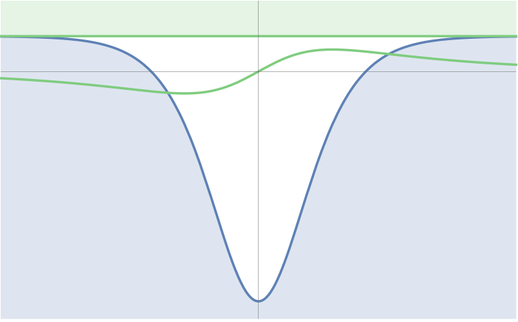
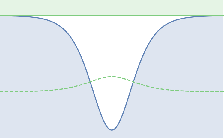
Figure 5: Spectrum of the differential operator in eq. (54) that coincides with the Pöschl-Teller potential well in Quantum Mechanics. The green band corresponds to the continuum spectrum. In the left (right) panel we show the parity odd (parity even) eigenfunction $q^{-}_{\lambda=0}(\tau)$ ($q^{+}_{\lambda=-8}(\tau)$). We do not show the parity even eigenfunction $q^{+}_{\lambda=0}(\tau)$ since it is not square-integrable.

Considering the eigenvalue equation $\mathcal{O}q_{\lambda}(\tau)=\lambda q_{\lambda}(\tau)$, they correspond to

$${\rm Odd\,eigenfunction:}~{}~{} \left\{q^{-}_{\lambda=0}(\tau)=\frac{\sinh(2\tau)}{\cosh^{3/2}(2\tau)}\right\}~{},$$ (56)

$${\rm Even\,eigenfunctions:}~{}~{} \left\{q^{+}_{\lambda=-8}(\tau)=\frac{1}{\cosh^{3/2}(2\tau)}~{},~{}~{}q^{+}_{\lambda=0}(\tau)=\frac{3-\cosh(4\tau)}{2\cosh^{3/2}(2\tau)}\right\}~{}.$$ (57)

At this stage, one would naïvely conclude that the differential operator in eq. (54) has one negative eigenvalue; this is, the reader might have noticed, in contradiction with eq. (55). The resolution of this conflict requires closer inspection, in particular, one needs to check the behaviour of the eigenfunctions at the boundaries in eq. (52) and the transformation property under parity. Let us start from the latter. Parity under $\tau\to-\tau$ $(\sim\eta\to-\eta)$ can be assigned to the perturbations in eq. (37), and carried on to the expression for $q$ in eq. (48) we see that it has odd parity, a reminder of the fact that the canonical transformation has ‘swapped’ momentum and coordinate. In eqs. (56,57), the only eigenfunction that is compatible with this requirement is $q^{-}_{\lambda=0}(\tau)$, with eigenvalue $\lambda=0$. Based on this parity argument, we therefore discard the eigenfunctions $q^{+}_{\lambda=-8}(\tau)$ and $q^{+}_{\lambda=0}(\tau)$. Second, we have to check the behaviour of the eigenfunctions at the boundaries in eq. (53). This can be done in two ways: $i)$ direct computation in eq. (53) where one finds that the boundary term cancel at $\tau\pm\infty$ for $q^{-}_{\lambda=0}$ (it does cancel at $\tau=0$ as well if one instead considers a half-wormhole), $ii)$ alternatively substitution of $q^{-}_{\lambda=0}$ in eq. (55) yields $0$ which comprises both bulk and boundary contributions in eq (53). In this regard, let us note that the even solutions put in eq. (55) yield $\infty$ when integrating around the throat of the wormhole. In this sense only $q^{-}_{\lambda=0}$ is an eigenfunction of both eq. (53) and eq. (55) which adds to the evidence in favour of the odd eigenfunction.

Notice that otherwise the presence of a zero eigenvalue can be inferred from the ‘time’-translation symmetry for the wormhole solution, as discussed in section 2.1.

All in all, we found that homogeneous scalar perturbations give a positive contribution to the fluctuation determinant in eq. (36). This result supports the interpretation of the wormhole as an instanton mediating tunneling transitions between degenerate vacua. Equipped with this result, we can now move to compute the effective potential generated by gravity.

Before proceeding, let us comment about the discrepancy with the result presented in [36] where a negative eigenvalue was found. The metric studied in [36] has the form $ds^{2}=N^{2}(\rho)d\rho^{2}+R^{2}(\rho)d\Omega^{2}$, with the wormhole solution corresponding to $N(\rho)=1$ and $R(\rho)=R_{\rm wh}(\rho)$, where $R_{\rm wh}(\rho)$ satisfies the equation $[R_{\rm wh}^{\prime}(\rho)]^{2}=1-1/R_{\rm wh}^{4}(\rho)$ with $R_{\rm wh}(\rho=0)=L$. The authors of [36] focused the analysis only on homogeneous perturbations; they defined the perturbed metric element as $ds^{2}=[1+n(\rho)]^{2}d\rho^{2}+[R_{\rm wh}(\rho)+r(\rho)]^{2}$, and – contrary to the explicit gauge-invariant formulation in this work – they fixed the gauge with the choice $n(\rho)=0$. This procedure may lead to incorrect results since perturbations are truncated before the gauge fixing, thus preventing from the possibility to fix all possible gauge degrees of freedom. Furthermore, in [36] the conformal factor problem was circumvented by using the Gibbons-Hawking-Perry rotation [37]. In synthesis, the ‘wrong’ negative kinetic term in the quadratic action for the perturbation $r(\rho)$ changes its sign as a consequence of the replacement $r\to\imath r$, with the new $r$ real. As already mentioned above, this is an ad hoc prescription without a clear physical interpretation, and its naïve application may lead to misleading results [38].

4 Effective potential from Euclidean wormholes

The non-linearly realized global $U(1)$ symmetry $\phi\to\phi+\alpha f_{a}$ is generated by the axion charge $\mathcal{Q}$. The ground state – corresponding to the bottom of the mexican hat potential – is degenerate along the angular direction, and vacua are described by continuously connected field configurations with minimum energy.

Half-wormholes induce quantum tunneling between classical vacuum states with different axion charge $\mathcal{Q}$. The situation is schematically represented in fig. 6. As Euclidean time passes by, in the presence of an instanton (anti-instanton) an observer on $\mathbb{R}^{3}$ experiences a change $\Delta\mathcal{Q}=-n$ ($\Delta\mathcal{Q}=+n$) since there is a net flux of axion charge equal to $+n$ ($-n$) through the wormhole throat [16, 17, 39].

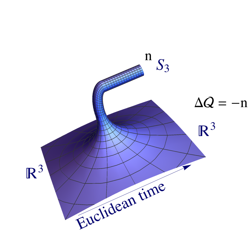
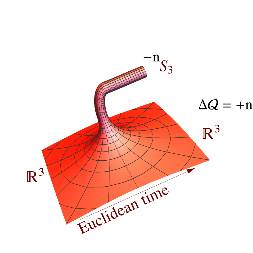
Figure 6: Half-wormholes as instantons in Euclidean space. In the left (right) panel we show an instanton (anti-instanton) mediating the topology change $\mathbb{R}^{3}\to\mathbb{R}^{3}\oplus S_{3}$, and carrying away an axion charge $+n$ ($-n$). The axion charge is overall conserved but an observer on $\mathbb{R}^{3}$ experiences, as Euclidean time passes by, a change $\Delta\mathcal{Q}=-n$ ($\Delta\mathcal{Q}=+n$). The non-conservation of the axion charge $\mathcal{Q}$ on $\mathbb{R}^{3}$ implies an explicit breaking of the symmetry it generates.

Eventually, we will consider the case with $n=1$, since the instanton action in eq. (19) is minimized. Consequently, from the point of view of the observer on $\mathbb{R}^{3}$, the axion charge is not conserved, and the associated symmetry explicitly broken down to the discrete gauge symmetry $\phi\to\phi+2k\pi f_{a}$, with $k\in\mathbb{Z}$, which remains intact in the presence of wormhole instantons, as discussed in section 2.1.

In the presence of wormhole instantons the situation is similar to that of a particle moving in a one-dimensional periodic potential. There are infinite classical minima at $x=j$, and each minimum corresponds to a degenerate ground state $|j\rangle$, as shown in fig. 7. Instantons can begin at any initial position, $x=j$, and go to the next one, $x=j+1$.

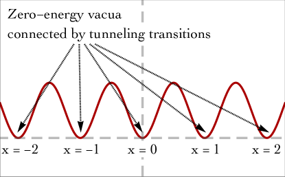
Figure 7: Periodic potential in Quantum Mechanics. Non-perturbative instanton solutions tunnel between classically degenerate vacua.

As a result of these tunneling transitions, the true vacuum of the system is a superposition of the degenerate ground states $|j\rangle$. It is instructive to work out this analogy in more detail. In particular, we can compute the probability for the tunneling process $|j\rangle\to|k\rangle$ summing over all the possible instanton and anti-instanton configurations. We find [22]

$$\langle k|e^{-HT}|j\rangle=\sqrt{\frac{\omega}{\pi}}e^{-\omega T/2}\sum_{n=0}^{\infty}\sum_{\bar{n}=0}^{\infty}\frac{1}{n!\bar{n}!}\left(Ke^{-\mathcal{S}_{0}}T\right)^{n+\bar{n}}\delta_{n-\bar{n},k-j}~{},$$ (58)

where $\omega\equiv V^{\prime\prime}(0)$, $K$ is the determinant factor describing quantum fluctuations around the classical instanton trajectory. Notice that for a single instanton/anti-instanton path with action $\mathcal{S}_{0}$ the contribution to the transition amplitude is [22]

$$\sqrt{\frac{\omega}{\pi}}e^{-\omega T/2}Ke^{-\mathcal{S}_{0}}~{}.$$ (59)

Eq. (58) include multi-instanton/anti-instanton solutions using the dilute-gas approximation. According to this approximation, strings of widely separated instantons and anti-instantons centered at $\tau_{1},\dots,\tau_{n}$, and satisfying the condition $-T/2<\tau_{1}<\dots<\tau_{n}<T/2$, are distributed arbitrarily along the time direction. Multi-instantons are not exact classical solutions, but they represent the leading term for the tunneling amplitude between distant wells. The contribution of a multi-instanton solution consisting in $n$ well-separated objects takes the same form as in eq. (59) but with $K\to K^{n}$, $\mathcal{S}_{0}\to n\mathcal{S}_{0}$. A similar result, with $n$ substituted by $\bar{n}$, is valid for an anti-instanton string. In addition, the integration over the freely-distributed position gives the factor

$$\int_{-T/2}^{T/2}dt_{n}\int_{-T/2}^{t_{n}}dt_{n-1}\dots\int_{-T/2}^{t_{2}}dt_{1}=\frac{T^{n}}{n!}~{}.$$ (60)

The Kronecker delta in eq. (58) takes into account the fact that the total number of instantons minus the total number of anti-instantons must equal the change in $x$ between the initial and final position eigenstates. Using the Fourier series representation

$$\delta_{a,b}=\int_{0}^{2\pi}\frac{d\bar{\zeta}}{2\pi}e^{\imath\bar{\zeta}(a-b)}~{},$$ (61)

we find

$$\langle k|e^{-HT}|j\rangle=\sqrt{\frac{\omega}{\pi}}e^{-\omega T/2}\int_{0}^{2\pi}\frac{d\bar{\zeta}}{2\pi}e^{\imath\bar{\zeta}(j-k)}\exp\left(2Ke^{-\mathcal{S}_{0}}T\cos\bar{\zeta}\right)~{}.$$ (62)

From eq. (62), we read the energy eigenstates (Bloch waves, using the language of solid state systems) and eigenvalues

$$|\zeta\rangle=\left(\frac{\omega}{\pi}\right)^{1/4}\frac{1}{\sqrt{2\pi}}\sum_{n}e^{-\imath n\zeta}|n\rangle~{},~{}~{}~{}~{}~{}E(\zeta)=\frac{\omega}{2}+2Ke^{-\mathcal{S}_{0}}\cos\zeta~{}.$$ (63)

The periodic potential contains a translation symmetry – analogue in rôle to the gauge symmetry $\theta\to\theta+2k\pi$ in eq. (2), left unbroken by wormhole instantons – that forces the eigenstates to be shift-invariant. It is indeed possible to introduce an operator $\mathcal{T}$ that generates an elementary translation $\mathcal{T}|j\rangle=|j+1\rangle$. $\mathcal{T}$ commutes with the Hamiltonian, and both operators can be diagonalized simultaneously. Each energy eigenstate in eq. (63) is characterized by an angle $\zeta$, eigenvalue of $\mathcal{T}$. It is indeed immediate to check that the states $|\zeta\rangle$ are eigenstates of $\mathcal{T}$, with $\mathcal{T}|\zeta\rangle=e^{\imath\zeta}|\zeta\rangle$.

A rigorous treatment in the context of wormhole physics was proposed in [39, 40, 41] (see also [42, 43, 44]).

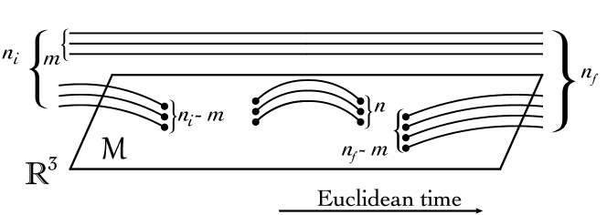
Figure 8: The computation of the transition amplitude between a state $|n_{i}\rangle$ with $n_{i}$ instantons to a state $|n_{f}\rangle$ with $n_{f}$ instantons requires the sum over all possible four-geometries. We show here the most general one [40, 41] which includes $m$ non-interacting wormholes, $n$ wormholes that are emitted and reabsorbed, $n_{i}-m$ half-wormholes in the initial and $n_{f}-m$ half-wormholes in the final state. From a local perspective, an effective potential on the space-time volume $\mathcal{M}$ is generated (see text for details).

The goal of these papers was to compute the influence of wormholes on physics at low energy, or at distances large compared to the thickness of the wormhole throat, $L$. The key idea is that at energy scales below $L^{-1}$ wormholes can be integrated out. In the resulting low-energy effective theory, the Lagrangian density takes the form

$$\mathcal{L}=\mathcal{L}_{0}\left[\Phi(x),\dots\right]+\sum_{i}\mathcal{O}_{i}\left[\Phi(x),\dots\right]\mathcal{A}_{i}~{}.$$ (64)

The second term captures the effect of topological fluctuations due to wormhole physics. In full generality, the sum over $i$ represents the possible presence of instantons of different type (for instance, instantons with different charge $\mathcal{Q}$). $\mathcal{O}_{i}(x)\equiv\mathcal{O}_{i}\left[\Phi(x),\dots\right]$ are generic functions of fields and their derivatives, and $\mathcal{A}_{i}$ are combinations of creation and annihilation operators describing emission and absorption of half-wormhole geometries of type $i$. Notice that $\mathcal{A}_{i}$ do not depend on space-time position since wormholes do not carry any momentum. Furthermore, wormholes do not carry away any quantity coupled to gauge fields, and $\mathcal{O}_{i}$ must be a Lorentz scalar, singlet under charge and color. However, as we learned in section 2, wormholes carry off axion charges, and as a consequence we expect the operator $\mathcal{O}_{i}(x)$ to transform non-trivially under the global $U(1)$ symmetry. We shall return on this point later.

Before proceeding, let us give a more quantitative understanding. The fact that integration over wormhole geometries gives rise to the structure in eq. (64) can be understood with an explicit computation [40, 41]. In practice, one can compute the probability for the transition between a state $|n_{i}\rangle$ with $n_{i}$ instantons to a state $|n_{f}\rangle$ with $n_{f}$ instantons, $\langle n_{f}|e^{-HT}|n_{i}\rangle$. For simplicity we do not distinguish here between instantons and anti-instantons, and we only consider instantons of unit charge. The computation should include a sum over all possible four-geometries, and in fig. 8 we show the most general of such configurations [40, 41]. This configuration includes $m$ disconnected wormholes that do not interact with the Euclidean space-time, and $n$ wormholes that are emitted and reabsorbed (see also fig. 2). The amplitude for this geometry is weighted by the factor $e^{-\mathcal{S}_{\rm inst}(2n+n_{f}+n_{i}-2m)}$, where $\mathcal{S}_{\rm inst}$ is the instanton action (with unit charge) computed in eq. (35). Furthermore, we indicate with $K\sqrt{g}d^{4}x$ the amplitude for inserting a single wormhole end in an infinitesimal volume of $\mathcal{M}$. For simplicity, we treat $K$ as a constant while, in general, it contains combinations of fields defined on $\mathcal{M}$. The final result – in analogy with eq. (58) – is

$$\langle n_{f}|e^{-HT}|n_{i}\rangle=\sum_{n=0}^{\infty}\sum_{m=0}^{{\rm min}(m_{i},n_{f})}\frac{\sqrt{n_{i}!\,n_{f}!}}{m!}\frac{(Ke^{-S_{\rm inst}}VT)^{2n+n_{i}+n_{f}-2m}}{2^{n}n!(n_{i}-m)!(n_{f}-m)!}~{},$$ (65)

where the volume factor $VT=\int_{\mathcal{M}}d^{4}x\sqrt{g}$ comes from an integration over the location of each instanton in the dilute gas approximation. The crucial observation in [40, 41] is that the same result presented in eq. (65) can be directly obtained from the left-hand side of eq. (65) using the Hamiltonian $H=Ke^{-S_{\rm inst}}V(a+a^{{\dagger}})$, after introducing creation and annihilation operators $a^{{\dagger}}$ and $a$ subject to the commutation relation $[a,a^{{\dagger}}]=1$, and defined by $|n\rangle=\sqrt{1/n!}(a^{{\dagger}})^{n}|0\rangle$. This result shows the validity of the assumption made in eq. (64).

The effective wormhole action – writing explicitly the presence of field operators $\mathcal{O}_{i}(x)$ in the spirit of eq. (64) – is therefore [39]

$$\mathcal{S}_{\rm wh} = \int d^{4}x\sqrt{g}\sum_{q}K_{q}e^{-\mathcal{S}_{\rm inst}}\left[\left(a^{{\dagger}}_{q}+a_{-q}\right)\mathcal{O}_{-q}(x)+\left(a^{{\dagger}}_{-q}+a_{q}\right)\mathcal{O}_{q}(x)\right]$$ (66)

$$= \int d^{4}x\sqrt{g}\sum_{q}K_{q}e^{-\mathcal{S}_{\rm inst}}\mathcal{O}_{S}(x)\left[\left(a^{{\dagger}}_{q}+a_{-q}\right)\exp\left(-\frac{\imath q\phi}{f_{a}}\right)+\left(a^{{\dagger}}_{-q}+a_{q}\right)\exp\left(\frac{\imath q\phi}{f_{a}}\right)\right]~{},$$

where $a^{{\dagger}}_{q}+a_{-q}$ ($a^{{\dagger}}_{-q}+a_{q}$) describes the creation of a half-wormhole with charge $q$ ($-q$) or, equivalently, the annihilation of a half-wormhole with charge $-q$ ($q$), as illustrated in fig. 9. The operators $a_{q}$ and $a_{q}^{{\dagger}}$ obey the usual commutation relations $[a_{q},a_{q^{\prime}}]=[a_{q}^{{\dagger}},a_{q^{\prime}}^{{\dagger}}]=0$ and $[a_{q},a_{q^{\prime}}^{{\dagger}}]=\delta_{qq^{\prime}}$.

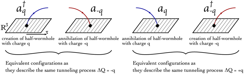
Figure 9: Creation and annihilation operators for instanton (blue) and anti-instantons (red) with commutation relations $[a_{q},a_{q^{\prime}}]=[a_{q}^{{\dagger}},a_{q^{\prime}}^{{\dagger}}]=0$ and $[a_{q},a_{q^{\prime}}^{{\dagger}}]=\delta_{qq^{\prime}}$.

As anticipated before, the operator $\mathcal{O}_{q}(x)$ transforms non-trivially under the global $U(1)$ symmetry, and it is possible to show that $\mathcal{O}_{q}(x)=\exp(\imath q\phi/f_{a})\mathcal{O}_{S}(x)$, where $\mathcal{O}_{S}(x)$ is a singlet. Under the symmetry transformation $\phi\to\phi+\alpha f_{a}$, it follows that $\mathcal{O}_{q}(x)\to\exp(\imath q\alpha)\mathcal{O}_{q}(x)$. As shown in [39], this transformation property ensures conservation of the global $U(1)$ charge when the sum over all possible topologies is considered (that is, for instance, $\mathbb{R}^{3}\oplus S_{3}$ for the creation of a single instanton, see fig. 6).

Finally, in order to derive a viable effective action, it is crucial to understand the rôle of the creation and annihilation operators in eq. (66). To this end, we can apply the lesson learned from Quantum Mechanics. At the beginning of section 3, we discussed the double-well potential. In perturbation theory, the system has two degenerate vacua $|\pm k\rangle$, and, after including instanton solutions, the Hamiltonian is diagonalized by $|+k\rangle\pm|-k\rangle$, with the true vacuum corresponding to the antisymmetric combination. This example shows that in the presence of instanton with no negative modes the quantum vacuum is constructed as a coherent superposition of classical vacua. The same conclusion remains valid for the periodic potential studied at the beginning of this section, with the true vacuum defined by the superposition in eq. (63). A similar situation arises in Quantum Field Theory. The QCD Lagrangian has a discrete set of degenerate classical minima, labelled by integers $n$ – dubbed winding number – and indicated with $|n\rangle$. Indeed, considering the Chern-Simons current $\mathcal{K}^{\rm CS}_{\mu}$ and the corresponding charge $\mathcal{K}^{\rm CS}$

$$\mathcal{K}^{\rm CS}_{\mu}=2\epsilon_{\mu\nu\alpha\beta}\left[A_{\nu}^{a}(\partial_{\alpha}A_{\beta}^{a})+\frac{g_{s}}{3}f_{abc}A_{\nu}^{a}A_{\alpha}^{b}A_{\beta}^{c}\right]~{},~{}~{}~{}~{}~{}~{}\mathcal{K}^{\rm CS}=\frac{g_{s}^{2}}{32\pi^{2}}\int\mathcal{K}_{0}^{\rm CS}(\vec{x},t)d^{3}\vec{x}~{},$$ (67)

it is possible to show that integer values $\mathcal{K}^{\rm CS}=n$ correspond to non-equivalent pure gauge field configurations with zero energy. Yang-Mills instantons tunnel between two such classical vacua, resulting in a non-zero matrix element $\langle n+1|e^{-HT}|n\rangle$. It means that in the presence of instantons the $|n\rangle$ vacua do not diagonalize the Hamiltonian, in analogy with eq. (62) and eq. (65). On the contrary, the true vacuum is the coherent superposition $|\theta\rangle=\sum_{n}e^{\imath n\theta}|n\rangle$. We expect the same situation in the presence of gravitational instantons. To this end, we introduce the operators $C_{q}\equiv a^{{\dagger}}_{q}+a_{-q}$ and $C^{{\dagger}}_{q}\equiv a^{{\dagger}}_{-q}+a_{q}$ with commutation relations $[C_{q},C_{q^{\prime}}]=[C^{{\dagger}}_{q},C^{{\dagger}}_{q^{\prime}}]=[C_{q},C^{{\dagger}}_{q^{\prime}}]=0$. It is possible to simultaneously diagonalize the operators $C_{q}$ and $C_{q}^{{\dagger}}$, and we define the eigenvalue equations $C_{q}|\alpha\rangle=\alpha_{q}|\alpha\rangle$, $C^{{\dagger}}_{q}|\alpha\rangle=\alpha_{q}^{*}|\alpha\rangle$.

Tunneling transitions bring the system in the coherent state $(a^{{\dagger}}_{-q}+a_{q})|\alpha\rangle=\alpha_{q}e^{\imath\delta_{q}}|\alpha\rangle$, defined in analogy with the harmonic oscillator as the eigenstate of the annihilation operator with complex eigenvalue $\tilde{\alpha}_{q}\equiv\alpha_{q}e^{\imath\delta_{q}}$. We can therefore replace creation and annihilation operators in eq. (66) with their eigenvalues, and obtain

where in the last line we explicitly wrote the most general combination of operators singlet under the $U(1)$ global symmetry. In eq. (69), we used as mass suppression scale the cutoff $1/L$, and $a$, $b$ and $\alpha_{q}$ are expected to be order one numbers. In eq. (68) the crucial point is that breaking effects are always proportional to the factor $e^{-\mathcal{S}_{\rm inst}}$, a trademark representing their non-perturbative origin. We remark that this point seems to be quite often overlooked in the literature, especially as far as phenomenological applications are concerned. Very often breaking effects generated by gravity are treated in a naïve way, along the line of the discussion outlined in the introduction, see eq. (4). On the contrary, the presence of the suppression factor $e^{-\mathcal{S}_{\rm inst}}$ plays a crucial rôle. In the second part of this paper we shall discuss in detail the most relevant phenomenological applications.

5 Phenomenological implications

In this section we discuss several phenomenological situations characterized by the presence of light axions with a decay constant such that non-perturbative gravity effects become relevant.

5.1 The QCD axion

We start discussing the implication of eq. (68) for the QCD axion. We consider only wormholes with unit charge, since they give the dominant contribution. The effective axion potential, including both QCD and non-perturbative gravitational contributions, is schematically given by

$$V(a)=\Lambda_{\rm QCD}^{4}\cos\left(\frac{\phi}{f_{a}}\right)+(1/L)^{4}e^{-\mathcal{S}_{\rm inst}}\cos\left(\frac{\phi}{f_{a}}+\delta_{1}\right)~{},$$ (70)

where we estimated the prefactor of the gravitational contribution to be of order $(1/L)^{4}$. This is nothing but an order-of-magnitude estimate based on dimensional arguments but it does not affect the final result since the exponential term $e^{-\mathcal{S}_{\rm inst}}$ dominates. In this regard, it is worth emphasizing the size of this suppression. Considering the benchmark value $f_{a}=10^{10}$ GeV for a QCD axion in the classical window, we have $\mathcal{S}_{\rm inst}\simeq 1.7\times 10^{8}$. The explicit breaking generated by gravity is therefore negligible for all purposes.

Let us explore the implications of eq. (70) in more detail. First, notice that we defined the axion field so that the low energy QCD contribution to the axion potential is minimized at $\phi=0$, and we redefined accordingly the phase $\delta_{1}$ in eq. (68). The phase shift $\delta_{1}$ arises from a mismatch between the gravitational and the low energy QCD term. In the absence of CP violation in the gravitational sector, the phase $\delta_{1}$ is just proportional to ${\rm Arg\,Det}[Y_{u}Y_{d}]$, with $Y_{u,d}$ the Yukawa matrices for up- and down-type quarks, and it arises from the chiral rotation needed to move the phase of the fermion mass matrix into the $\theta$-term. In the following, we interpret $\delta_{1}$ as an arbitrary order one phase.

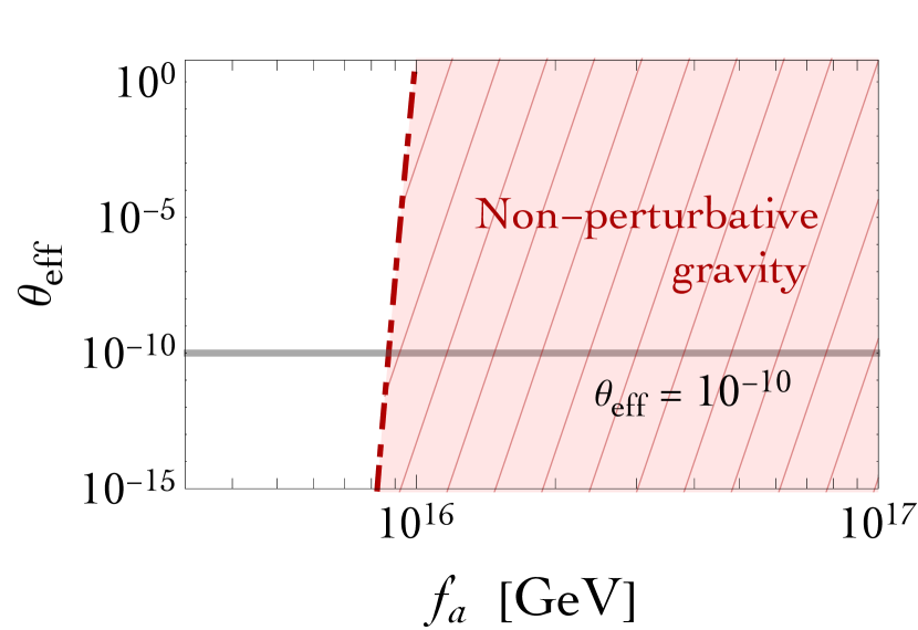
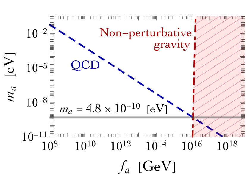
Figure 10: Non-perturbative gravity corrections (red dot-dashed line) on $\theta_{\rm eff}$ (left panel) and the axion mass $m_{a}$ (right panel) as a function of the axion decay constant $f_{a}$. In the regions shaded in red non-perturbative gravity dominates. In the right panel, the dashed blue line represents the contribution to the axion mass generated by QCD, computed according to [59].

The effect of the gravitational correction is twofold: It shifts the axion mass, and produces a non-zero $\theta_{\rm eff}$. We find

$$m_{a}^{2} \simeq \frac{\Lambda_{\rm QCD}^{4}}{f_{a}^{2}}+\frac{(1/L)^{4}}{f_{a}^{2}}e^{-\mathcal{S}_{\rm inst}}~{},$$ (72)

$$\theta_{\rm eff} \simeq \frac{(1/L)^{4}}{\Lambda_{\rm QCD}^{4}}\,\sin\delta_{1}\,e^{-\mathcal{S}_{\rm inst}}~{}.$$ (73)

where we remind the reader that the action scales with $M_{\rm Pl}/f_{a}$. The gravitational correction to the axion mass features a very interesting property if compared with the contribution generated by QCD. As $f_{a}$ increases, the QCD axion mass $\Lambda_{\rm QCD}^{4}/f_{a}^{2}$ decreases but the gravitational term becomes more and more important, and eventually it overcomes the former. This means that we expect a lower bound on the axion mass. This is shown in the right panel of fig. 10 where we shaded in red the region in which non-perturbative gravitational corrections dominate. We find the lower bound on the axion mass (or, equivalently, the upper bound on the axion decay constant)

In the left panel of fig. 10 we show the impact of the non-zero $\theta_{\rm eff}$ in eq. (73). For reference, we consider the experimental bound $\theta_{\rm eff}<10^{-10}$ (horizontal gray line). We find that if $f_{a}\gtrsim 10^{16}\,{\rm GeV}$ then the contribution induced by gravity becomes too large. Notice that, by accident, the bounds on $f_{a}$ extracted from $m_{a}$ and $\theta_{\rm eff}$ are of the same order, and assuming $\delta_{1}=0$ does not change quantitatively our conclusion.

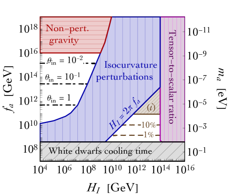
Figure 11: QCD axion parameter space (see text for details). The region shaded in red with horizontal meshes is excluded by non-perturbative gravitational effects, eq. (74).

In fig. 11 we show the impact of the bound in eq. (74) on the QCD axion parameter space. As customary, the condition $f_{a}\lessgtr H_{I}/2\pi$, with $H_{I}$ the Hubble expansion rate at the end of inflation distinguishes between the cases in which the PQ symmetry is broken before ($>$) or after ($<$) the end of inflation. The first possibility defines the so-called anthropic axion window, in which the possibility to reproduce the observed dark matter relic density $\Omega_{a}h^{2}\simeq 0.1$ relies on a fine-tuned choice of the initial misalignment angle $\theta_{in}$ (black dot-dashed lines in fig. 11 for different $\theta_{in}$). Notice that a substantial part of the anthropic axion window is excluded by the presence of axion isocurvature perturbations in the early Universe (blue region with vertical meshes) that we compute following [60, 61] (see also [62, 63] for recent progress for non-standard cosmologies and generalization to axion-like particles). The region $f_{a}<H_{I}/2\pi$ defines the classical axion window. In the region (i) shaded in brown with diagonal meshes $\Omega_{a}h^{2}>0.1$, and the Universe is over-closed. The dashed brown lines reproduce $1\%$ and $10\%$ of the observed dark matter abundance. In this region a sizable contribution from decay of topological defects is expected [64]. For completeness, we also show the region excluded by white dwarf cooling time [65] and upper limit on the tensor-to-scalar ratio [66]. The bound in eq. (74) applies in the anthropic axion window, and disfavors a region of the parameter space (shaded in red with horizontal meshes) previously allowed. We remark that the bound in eq. (74) was derived without specific assumption but only considering minimal coupling of the axion field with Einstein gravity.

We now move to briefly discuss few scenarios of phenomenological relevance in which non-perturbative gravitational corrections to the mass of the QCD axion may play an important rôle.

5.1.1 QCD axions and black hole superradiance

Spin and mass measurements of stellar-size black holes exclude the QCD axion mass window [67]

$$6\times 10^{-13}\lesssim m_{a}\,[{\rm eV}]\lesssim 2\times 10^{-11}~{},$$ (75)

corresponding to $3\times 10^{17}\lesssim f_{a}\,[{\rm GeV}]\lesssim 10^{19}$. This is because superradiance effects become efficient [68, 69] when the Compton wavelength of the axion is comparable with the horizon size of the black hole. The axionic field forms a quasi-stationary configuration around the black hole at the expense of its rotational energy, giving birth to a quasi-bound system that shares remarkable similarities – such as energy orbitals and level transitions – with the hydrogen atom. From $\lambda_{\rm Compton}=h/m_{a}c\sim R$, we have

$$m_{a}\sim 6\times 10^{-12}\left(\frac{30\,{\rm km}}{R}\right)\,{\rm eV}~{},$$ (76)

where $R$ is the typical radius of a stellar-mass black hole, thus justifying the mass range excluded in eq. (75). At the two sides of this interval, and within the mass range $m_{a}=[10^{-14},10^{-10}]$ eV, stellar black hole superradiance in the presence of the QCD axion may produce in the next few years spectacular signatures – both direct and indirect – in gravitational wave detectors such as Advanced LIGO [70, 71]. Indirect signatures refer to the observation of gaps in the spin-mass distribution of final state black holes produced by binary black hole mergers. Direct signatures refer to monochromatic gravitational wave signals produced during the dissipation of the scalar condensate after the superradiant condition is saturated.

As far as direct signatures are concerned, a careful assess of the detection prospects in Advanced LIGO and LISA was recently proposed in [72, 73]. The outcome of the analysis is that, considering optimistic astrophysical models for black hole populations, the gravitational wave signal produced by superradiant clouds of scalar bosons with mass in the range $m_{a}=[2\times 10^{-13},10^{-12}]$ eV is observable – i.e. it is characterized by a signal-to-noise ratio larger than the experimental threshold – by Advanced LIGO. Notice that this region seems to be ruled out if one considers at face value the bound in eq. (75). However, it is worth emphasizing that the bound in eq. (75) is most likely only indicative since it is based on black hole spin measurements that are extracted indirectly from X-ray observations of accretion disks in X-ray binaries. We only have very few of such measurements at our disposal, and it is difficult to extract a bound with significant statistical confidence. The discussion of this matter however escapes the scope of the present work.

As clear from the right panel of fig. 10 and from the parameter space in fig. 11, the QCD axion in the mass range $m_{a}=[10^{-14},10^{-10}]$ eV violates the bound in eq. (74), and fits into a region where non-perturbative gravitational effects dominate over QCD. We therefore conclude that – working under the very same hypothesis, that is an axion minimally coupled to Einstein gravity – the phenomenologically interesting mass range $m_{a}=[10^{-14},10^{-10}]$ eV motivated by black hole superradiance is theoretically forbidden for the QCD axion. This is not, of course, a lapidary conclusion. To be more optimistic, observing the QCD axion in connection with black hole mergers at the Advanced LIGO could imply an evidence for modifications of Einstein gravity. Alternatively, a scalar boson different from the QCD axion could still leave its imprint in the texture of gravitational wave signatures.

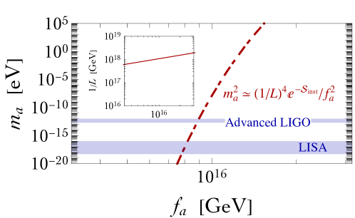
Figure 12: Gravitational mass generated by non-perturbative Euclidean wormholes as a function of the Goldstone boson decay constant $f_{a}$. In the inset plot, we show, in the same interval of $f_{a}$, the inverse of the wormhole size $L$ (see eq. (17)). The horizontal blue lines represent the mass range favored by the analysis in [72, 73] considering both Advanced LIGO ($m_{a}=[2\times 10^{-13},10^{-12}]$ eV) and LISA ($m_{a}=[5\times 10^{-19},5\times 10^{-16}]$ eV) gravitational wave detectors.

In this last case, the mass term generated by gravity can be used to justify the lightness of the scalar boson. By turning off the QCD contribution in eq. (72), we show the gravitational mass $m_{a}^{2}\simeq(1/L)^{4}e^{-\mathcal{S}_{\rm inst}}/f_{a}^{2}$ in fig. 12. Clearly, if $f_{a}\simeq 10^{16}$ GeV it is possible to span, thanks to the exponential factor $e^{-\mathcal{S}_{\rm inst}}$ a large range of allowed values, including the regions favored by the analysis in [72, 73].

5.1.2 Axion stars as black hole seeds

The idea is to consider axion stars as black hole seeds, which are supermassive in the case of ultralight axions [74]. By studying numerically the collapse of axion stars in the context of general relativity, the authors of [74] identified the critical value of the axion decay constant $f_{\rm TP}\sim 0.06\,M_{\rm Pl}$ above which black hole formation occurs. The mass of the typical black hole formed from axion star collapse is $M_{\rm BH}\sim 3.4\left(f_{a}/0.12\,M_{\rm Pl}\right)^{1.2}M_{\odot}$.

As before, the condition $f_{a}\gtrsim f_{\rm TP}\sim 0.06\,M_{\rm Pl}$ is not compatible with the bound in eq. (74). We stress that this bound was derived considering a QCD axion minimally coupled to Einstein gravity, therefore without any additional assumptions compared to the ones in [74]. Said differently, it would be interesting to include in the analysis of [74] non-perturbative gravitational corrections to the axion potential since they play a relevant rôle in the region of parameter space in which black hole formation may occur.

5.2 Ultralight scalars as cosmological dark matter

Dark matter must behave sufficiently classically to be confined on galaxy scales. If we suppose dark matter to be a boson with mass $m_{a}$ and velocity $v$, we can require to behave classically down to the typical size of Milky Way satellite galaxies, and obtain the condition

$$\lambda_{\rm De\,Broglie}=\frac{1}{m_{a}v}\lesssim 1~{}{\rm kpc}~{}~{}~{}~{}\Longrightarrow~{}~{}~{}~{}m_{a}\gtrsim 10^{-22}\,\left(\frac{120\,{\rm km/s}}{v}\right)\,{\rm eV}~{}.$$ (77)

For a typical halo with size $R\sim{\rm kpc}$, and mass $M\sim 10^{9}\,M_{\odot}$, we expect a virial velocity $v\sim\sqrt{G_{N}M/R}\sim 70$ km/s. From eq. (77), we extract a lower limit for the mass of bosonic dark matter of about $10^{-22}$ eV. The dark matter saturating this value is known as fuzzy dark matter (FDM) [75]. This kind of ultralight dark matter could form a Bose-Einstein condensate on galactic scales, providing a possible solution to the tensions that arise when the standard cold dark matter paradigm is probed into the deep non-linear regime at redshift $z\sim 0$ [76, 77, 78]. Apart from this motivation, an ultralight dark matter condensate features peculiar observational astrophysical properties, and it catalyzed increasing attention in the dark matter community (see, e.g.,  [84, 82, 81, 79, 83, 80, 85, 86]).

From a particle physics perspective, the extreme lightness of the FDM is well suited by an axion-like particle. Furthermore, reproducing the observed value of relic abundance via the misalignment mechanism gives a clue about the value of its decay constant $f_{a}$.

For completeness, let us quickly sketch the computation. We consider here an axion-like field $a(t,\vec{x})=f_{a}\theta(t,\vec{x})$ with potential $V(a)=\mu^{4}\left(1-\cos\theta\right)$. In the Friedmann-Robertson-Walker cosmology $ds^{2}=-dt^{2}+R^{2}(t)d\vec{x}^{2}$ the evolution of the axion field is given by $\ddot{a}(t,\vec{x})+3H\dot{a}(t,\vec{x})-\triangle a(t,\vec{x})/R^{2}+dV(a)/da=0$, where $H\equiv\dot{R}/R$, and the dot indicates derivative w.r.t. time. Neglecting higher order in the potential, we have $\ddot{a}(t,\vec{x})+3H\dot{a}(t,\vec{x})-\triangle a(t,\vec{x})/R^{2}+m_{a}^{2}a(t,\vec{x})=0$, with $m_{a}^{2}\equiv\mu^{4}/f_{a}^{2}$. As customary, we can define the time $t_{1}$ at which the condition $m_{a}=3H(t_{1})$ is satisfied. Notice that for simplicity we are considering an axion mass that is, to a first approximation, temperature-independent. The time $t_{1}$ separates two regimes.

For $t<t_{1}$, we can neglect the mass term, $H\gg m_{a}$. Introducing the Fourier decomposition $a(t,\vec{k})=\int d^{3}\vec{x}e^{i\vec{k}\cdot\vec{x}}a(t,\vec{x})$ we obtain $\ddot{a}(t,\vec{k})+3H\dot{a}(t,\vec{k})-(k^{2}/R^{2})a(t,\vec{k})=0$. The Fourier modes $a(t,\vec{k})$ separate into modes outside (that is for $k/R\ll H$) and inside (that is for $k/R\gg H$) the horizon. Inside the horizon, we can not neglect the $k^{2}/R^{2}$ term. Solving the equation of motion for these modes, it is possible to show that the corresponding solutions oscillate with frequency $k/R$, and the amplitude decreases with time as $1/R$. The modes that are confined inside the horizons until $t\simeq t_{1}$ can therefore be neglected. As far as the modes outside the horizon are concerned, we can neglect the $k^{2}/R^{2}$ term, and the equation of motion is solved by $a(t,\vec{k})=c_{1}(\vec{k})+c_{2}(\vec{k})t^{-1/2}$. The modes that are confined outside the horizon until $t\simeq t_{1}$ are therefore frozen at some constant initial value, and they are collectively called zero modes $a_{0}$.

Let us now move to discuss the second regime, $t\gtrsim t_{1}$, focusing on the zero modes. When the axion mass becomes non-negligible, the evolution of the zero modes is described by the equation $\ddot{a}_{0}+3H\dot{a}_{0}+m_{a}^{2}a_{0}=0$. The zero modes, previously frozen, at $t\gtrsim t_{1}$ start oscillate with frequency set by $m_{a}$. From the definition of axion energy density $2\rho_{a_{0}}=\dot{a}_{0}^{2}+m_{a}^{2}a_{0}^{2}$ we find, using the equation of motion, $\dot{\rho}_{a_{0}}=-3H\dot{a}_{0}^{2}$. Since $a_{0}$ oscillates with period $m_{a}$, we can average over an oscillation, and estimate $\dot{a}_{0}\simeq m_{a}a_{0}$. Consequently, $\rho_{a_{0}}\simeq m_{a}^{2}a_{0}^{2}$ and $\dot{\rho}_{a_{0}}\simeq-3H\rho_{a_{0}}$. After integration, the latter equation gives the scaling $\rho_{a_{0}}(t)\sim m_{a}/R^{3}(t)$. This is the key argument defining the physics of the misalignment mechanism: During the cosmological evolution of the axion field, for $t\gtrsim t_{1}$ the number of axions in a comoving volume is conserved. We can therefore write the energy density stored in the axion zero modes today as

$$\rho_{a_{0}}(t_{0})=\rho_{a_{0}}(t_{1})\left[\frac{R(t_{1})}{R(t_{0})}\right]^{3}~{},~{}~{}~{}~{}\rho_{a_{0}}(t_{1})\simeq m_{a}^{2}f_{a}^{2}\theta_{in}^{2}~{},$$ (78)

where the dependence from the so-called initial misalignment angle $\theta_{in}$ is manifest.

The rest of the computation makes use of some basic thermodynamic concepts to rephrase eq. (78) in terms of observable quantities. From entropy conservation, $g_{*}^{s}(T)R^{3}T^{3}={\rm const}$, we have

$$\left[\frac{R(t_{1})}{R(t_{0})}\right]^{3}=\frac{s(T_{0})}{\frac{2\pi^{2}}{45}g_{*}(T_{1})T_{1}^{3}}~{},~{}~{}~{}~{}~{}{\rm with}~{}~{}~{}s(T_{0})=\frac{4}{3}\left[\frac{g_{*}^{s}(T_{0})}{g_{*}(T_{0})}\right]\left(\frac{\rho_{R}(T_{0})}{T_{0}}\right)~{},$$ (79)

where $h\equiv H_{0}/(100\,{\rm km/s/Mpc})$, with $H_{0}=67.8\,{\rm km/s/Mpc}$ [87], is the reduced Hubble constant, $T_{1}$ is the temperature at time $t_{1}$, $T_{0}=2.726$ ^∘K is the present temperature of the Universe, $\rho_{\rm crit}=3H_{0}^{2}/8\pi G_{N}$ is the critical energy density, $g_{*}(T)$ ($g_{*}^{s}(T)$) is the effective number of degrees of freedom (effective number of degrees of freedom in entropy) at temperature $T$, and $\rho_{R}(T_{0})$ is the present energy density in radiation. In eq. (79) $s(T_{0})$ is the entropy density at present time, and the relation between $s(T_{0})$ and $\rho_{R}(T_{0})$ follows from

$$s(T)=\frac{2\pi^{2}}{45}g_{*}^{s}(T)T^{3}~{},~{}~{}~{}~{}\rho_{R}(T)=\frac{\pi^{2}}{30}g_{*}(T)T^{4}~{}.$$ (80)

The energy density in radiation can be estimated from the two Planck measurements [87] of the current matter density $\Omega_{m}$ and the redshift of radiation-matter equality $z_{eq}$. From $\rho_{m}(z_{eq})=\rho_{R}(z_{eq})$, which is equivalent to $\Omega_{m}(z_{eq}+1)^{3}=\Omega_{R}(z_{eq}+1)^{4}$, and using $\Omega_{m}=0.3$, $z_{eq}=3365$, it follows that $\Omega_{R}h^{2}\simeq 4.3\times 10^{-5}$.

The value of $T_{1}$ follows from the condition $m_{a}=3H(t_{1})$ taking into account that we can write the Hubble parameter as a function of the temperature as $H(T)=\sqrt{\pi^{2}g_{*}(T)/90M_{\rm Pl}^{2}}T^{2}$. Parametrically, we have the relation $M_{\rm Pl}m_{a}\simeq T_{1}^{2}$. For a FDM candidate with $m_{a}\simeq 10^{-22}$ eV, it follows that $T_{1}\simeq 10^{3}$ eV. At such small value of the temperature, we can approximate $g_{*}(T_{1})\approx 1$. Furthermore, we also have $g_{*}(T_{0})\simeq g_{*}^{s}(T_{0})$.

All in all, defining $\Omega_{a}\equiv\rho_{a_{0}}(t_{0})/\rho_{\rm crit}$, and assuming $\theta_{\rm in}\simeq 1$, we find the parametric order-of-magnitude scaling

$$\Omega_{a}h^{2}\approx 0.1\,\left(\frac{f_{a}}{10^{17}\,{\rm GeV}}\right)^{2}\left(\frac{m_{a}}{10^{-22}\,{\rm eV}}\right)^{1/2}~{}.$$ (81)

Eq. (81) points towards a very specific interplay between $f_{a}$ and $m_{a}$, and it is interesting to further investigate its origin. In [85] this relation was justified referring to string theory models in which one expects an explicit breaking of the axionic shift symmetry due to the existence of worldsheet or membrane instantons [88]. Even without invoking string theory constructions, we point out that the mass term generated by gravity in eq. (68) provides a nice explanation for the relic abundance in eq. (81). Indeed, using $m_{a}^{2}\simeq(1/L)^{4}e^{-\mathcal{S}_{\rm inst}}/f_{a}^{2}$, the observed abundance can be reproduced with $f_{a}\simeq 8\times 10^{15}$ GeV and $m_{a}\simeq 2.5\times 10^{-18}$ eV. Notice that this value falls within the mass range that will be explored by the LISA gravitational wave interferometer, see fig. 12. This is an interesting observation, since it shows that a dark matter candidate with nothing more than gravitational interactions may explain in a natural way the lightness of its mass.

We finally note that, as fig. 12 shows, a value of the axion decay constant above $f_{a}\simeq 10^{16}$ GeV would generate an unacceptably large contribution in eq. (81).

6 Comments on the rôle of possible UV completions

In this section we discuss possible UV completions of the axion Goldstone mode, and their consequences on wormhole physics.

6.1 Dynamical radial mode

We start our investigation considering the simplest UV completion of the axion theory. This is the case of a $U(1)$ global symmetry that is spontaneously broken by the VEV $\langle|\Phi|\rangle=f_{a}/\sqrt{2}$ of a complex scalar field $\Phi(x)=[f(x)/\sqrt{2}]e^{\imath\phi(x)/f_{a}}$. The mexican hat potential responsible for the spontaneous symmetry breaking is $V(f)=\lambda(f^{2}-f_{a}^{2})^{2}/4$. The radial field $f(x)$ gets a mass $M_{f}^{2}=\lambda f_{a}^{2}$. The physics discussed in the previous sections corresponds to the case in which the radial mode does not participate in the dynamics, and its value remains frozen at $f=f_{a}$. We expect this situation to be strictly true if $M_{f}>1/L$. For the critical value $f_{a}\simeq 10^{16}$ GeV that we identified in section 5.1, we have $1/L\simeq 10^{18}$ GeV. It is therefore hard to imagine that the radial field $f$ plays no dynamical rôle, since we expect its mass – for reasonable small coupling $\lambda$ – to lie below the scale set by the wormhole throat. In order to validate our conclusions, it is necessary to generalize the wormhole solutions, and compute their action, to the case in which $f$ is a dynamical field [15, 95]. In order to make contact with the existing literature, we look for spherically symmetric solutions, and we use the Euclidean metric ansatz $ds^{2}=dr^{2}+R^{2}(r)d\Omega^{2}_{3,1}$. The Ricci scalar is $\mathcal{R}=-6[-1+(R^{\prime})^{2}+RR^{\prime\prime}]/R^{2}$, and the Einstein field equations, together with the equation of motion for the radial field $f$, are [17, 95]

$$(R^{\prime})^{2} = 1-\frac{8\pi R^{2}}{3M_{\rm Pl}^{2}}\left[-\frac{(f^{\prime})^{2}}{2}+V(f)+\frac{n^{2}}{8\pi^{4}f^{2}R^{6}}\right]~{},$$ (82)

$$-1+(R^{\prime})^{2}+2RR^{\prime\prime} = -\frac{8\pi R^{2}}{M_{\rm Pl}^{2}}\left[\frac{(f^{\prime})^{2}}{2}+V(f)-\frac{n^{2}}{8\pi^{4}f^{2}R^{6}}\right]~{},$$ (83)

$$f^{\prime\prime}+\frac{3R^{\prime}}{R}f^{\prime} = \frac{dV}{df}-\frac{n^{2}}{4\pi^{4}f^{3}R^{6}}~{},$$ (84)

where we already substituted $f^{2}(\theta^{\prime})^{2}=n^{2}/4\pi^{4}f^{2}R^{6}$, with $n$ the quantized axion charge along the wormhole throat. Instead of eqs. (82,83), in our numerical investigation we found more useful to use the combination $R^{\prime\prime}=(4\pi R/3M_{\rm Pl}^{2})[-2(f^{\prime})^{2}-2V(f)+n^{2}/2\pi^{4}f^{2}R^{6}]$. We introduce the dimensionless variables [15, 95]

$$\rho\equiv rM_{\rm Pl}\sqrt{\frac{3\lambda}{8\pi}}~{},~{}~{}~{}~{}A\equiv RM_{\rm Pl}\sqrt{\frac{3\lambda}{8\pi}}~{},~{}~{}~{}~{}F\equiv\frac{f}{M_{\rm Pl}}\sqrt{\frac{8\pi}{3}}~{},$$ (85)

and the differential equations become

$$A^{\prime\prime}=\frac{A}{2}\left[-2(F^{\prime})^{2}-\frac{1}{2}(F^{2}-F_{a}^{2})^{2}+\frac{4Q}{F^{2}A^{6}}\right]~{},~{}~{}~{}~{}~{}~{}~{}F^{\prime\prime}+\frac{3A^{\prime}}{A}F^{\prime}=F(F^{2}-F_{a}^{2})^{2}-\frac{2Q}{F^{3}A^{6}}~{},$$ (86)

with $Q\equiv n^{2}\lambda^{2}/8\pi^{4}$. Finally, in terms of the dimensionless variables defined in eq. (85), the action – including the Gibbons-Hawking-York boundary term – reads

$$\mathcal{S}=\frac{2\pi^{2}}{\lambda}\int_{0}^{\infty}d\rho\left[A^{3}(F^{\prime})^{2}+2AA^{\prime}\left(1-A^{\prime}\right)\right]~{}.$$ (87)

We solve eq. (86) by means of a shooting method that we validate against the results of [15].

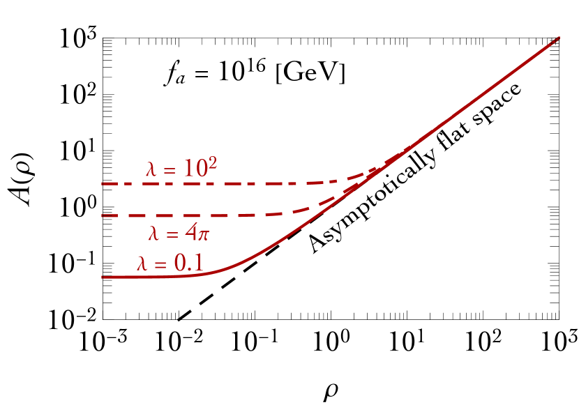
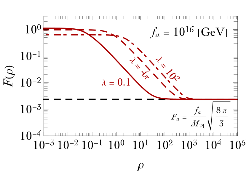
Figure 13: Left panel. Wormhole geometry in terms of the rescaled metric factor $A(\rho)$ as a function of the dimensionless coordinate $\rho$ for different values of $\lambda$. The dashed black line refers to the flat Euclidean limit $A(\rho)=\rho$. Right panel. Rescaled radial field $F(\rho)$ as a function of the dimensionless coordinate $\rho$ for different values of $\lambda$. The dashed black line refers to the VEV $F_{a}$.

The procedure goes as follows. First, for a given initial guess for $F(\rho=0)$ we compute $A(0)$ from the equation $A^{4}(0)-A^{6}(0)[F(0)^{2}-F_{a}^{2}]^{2}/4-Q/F^{2}(0)=0$. Second, we solve the system in eq. (86) with the four boundary data $F(0)$, $A(0)$, $A^{\prime}(0)=0$, $F^{\prime}(0)=0$. Finally, we check the asymptotic condition $F(\infty)=F_{a}$, and we tune the initial guess $F(0)$ until we find it satisfied. We show our result in fig. 13, where we focused on the critical value $f_{a}=10^{16}$ GeV and wormhole with unit charge $n=1$. In the left (right) panel we show the dimensionless metric function $A(\rho)$ (the dimensionless radial field $F(\rho)$) as a function of the rescaled distance $\rho$ for three different values of $\lambda$. As far as the geometry is concerned, we see that, asymptotically, the solution recovers the flat space $A(\rho)=\rho$ while for small $\rho$ deviations describing the wormhole geometry emerge. Going through the wormhole throat, the radial field $F(\rho)$ substantially deviates w.r.t. the its asymptotic value $F_{a}$. As expected, including the radial mode with mass $M_{f}<1/L$ as dynamical degree of freedom alters the wormhole solution found for non-propagating $f$. It is therefore important to quantify such deviation by computing the value of the action in eq. (87).

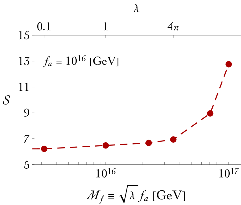
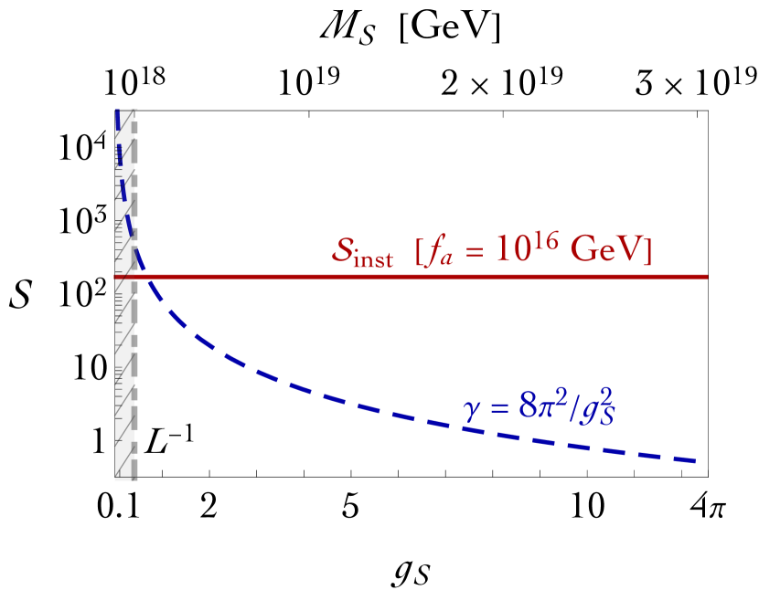
Figure 14: Left panel. On-shell action in eq. (87) as a function of the mass of the radial mode $M_{f}$. Right panel. Instanton action as a function of the string coupling $\mathrm{g}_{S}$. On the top x-axis we show the value of the string mass scale $M_{S}$ computed in eq. (93). In solid red, we show the on-shell action $\mathcal{S}_{\rm inst}$ for the instanton at the critical value $f_{a}=10^{16}$ GeV. The blue dashed line represents the topological contribution $\gamma=8\pi^{2}/\mathrm{g}_{S}^{2}$. The region shaded in gray corresponds to $M_{S}<L^{-1}$.

We show our result in the left panel of fig. 14, in which we plot the on-shell action $\mathcal{S}$ as a function of the mass of the radial mode $M_{f}$. From eq. (35), we have that the instanton action with the radial mode frozen at $f_{a}=10^{16}$ GeV is $\mathcal{S}_{\rm inst}\simeq 170$. Including the dynamics of the radial mode results in a net decrease of the action, in agreement with the result of [15]. Let us give a qualitative understanding of this effect. As derived in eq. (19), the wormhole action is proportional to $M_{\rm Pl}^{2}L^{2}$, and it decreases if the size of its throat gets smaller. The inclusion of a light dynamical radial mode has precisely this effect, as can be seen from the left panel in fig. 14: Going towards smaller values of $\lambda$ the size of the wormhole shrinks, and, consequently, the wormhole action decreases. For illustrative purposes, in fig. 14 we extend the plot to large values of $\lambda$ in order to show that, as $M_{f}$ moves towards the threshold $1/L$ above which it can be safely integrated out, the action increases.

The inclusion of the radial mode in the $U(1)$ model shows that the presence of dynamical degrees of freedom belonging to the UV completion of the axion Lagrangian does not weaken the strength of the non-perturbative global symmetry breaking induced by gravity. On the contrary, the total action in fig. 14 is significantly smaller if compared to the one in which the radial mode does not fluctuate around its VEV.

We therefore conclude that the bound derived in section 5.1 presumably represents a conservative estimate, since extra dynamics related to the UV completion of the axion Lagrangian may even strengthen the global symmetry breaking.

6.2 Higher-curvature operators and string theory

In this section we explore the impact of higher-curvature operators on the wormhole solution. To be more concrete, we include the Gauss-Bonnet term

$$\Delta\mathcal{S}_{\rm E}=-\frac{\gamma}{32\pi^{2}}\int d^{4}x\sqrt{g}\left(\mathcal{R}_{\mu\nu\lambda\delta}\mathcal{R}^{\mu\nu\lambda\delta}-4\mathcal{R}_{\mu\nu}\mathcal{R}^{\mu\nu}+\mathcal{R}^{2}\right)~{},$$ (88)

that represents the $4^{\rm th}$ order in the derivative expansion of the gravitational action. We limit our analysis to the Gauss-Bonnet term since it is the unique ghost-free quadratic curvature invariant [96]. Furthermore, as we shall discuss later, the presence of the effective higher-curvature correction in eq. (88) is a peculiar prediction of many string theories – bosonic [96], heterotic [97], and type-I string [98] (while it vanishes in type-II superstring theory [99]).

In $D=4$ dimensions, the Gauss-Bonnet term reduces to a total derivative. As a consequence, it does not enter in the equation of motion but it gives a non-vanishing topological contribution to the wormhole action. Before proceeding, we notice that the validity of the derivative expansion in the gravitational action imposes the cutoff $\Lambda\sim M_{\rm Pl}/\sqrt{\gamma/4\pi}$. It is therefore natural to require the condition $\Lambda>1/L$, in order to ensure the validity of the derivative expansion all the way down the wormhole throat. We find that this condition corresponds to

$$\gamma<\frac{4M_{\rm Pl}}{\sqrt{3\pi}f_{a}}~{}.$$ (89)

To fix ideas, if $f_{a}=10^{16}$ GeV we have $\gamma\lesssim 1600$. We now compute the value of the Gauss-Bonnet term on the wormhole solution. Using the metric in eq. (21), a direct computation gives

$$\mathcal{R}_{\mu\nu\lambda\delta}\mathcal{R}^{\mu\nu\lambda\delta}-4\mathcal{R}_{\mu\nu}\mathcal{R}^{\mu\nu}+\mathcal{R}^{2}=\frac{24\alpha^{\prime}(-1+\alpha^{2})}{r^{3}\alpha^{5}}~{},$$ (90)

and the action in eq. (88) gives

$$\Delta\mathcal{S}_{\rm E}=\frac{3\gamma}{2}\int_{L}^{\infty}\frac{\alpha^{\prime}(1-\alpha^{2})}{\alpha^{4}}=\frac{3\gamma}{2}\left|\frac{1}{\alpha}-\frac{1}{3\alpha^{3}}\right|_{r=L}^{r=\infty}=\gamma~{}.$$ (91)

Let us focus on the case of the QCD axion, discussed in section 5.1. At the critical value $f_{a}=10^{16}$ GeV, the instanton action is $\mathcal{S}_{\rm inst}\simeq 170$. As a rule of thumb, we can say that if $\gamma\gtrsim 170$ the higher-curvature topological correction due to the Gauss-Bonnet term in eq. (91) significantly alters the instanton action, increasing its value, and making its impact on axion physics harmless. Although qualitatively correct, the real point here is to understand the physical implications of this numerical condition. On a pure gravitational ground, $\gamma$ is nothing but a dimensionless number, and it seems difficult to justify the relation $\gamma\gtrsim 170$. Reinterpreting the effective action in eq. (88) having in mind the UV physics responsible for its generation would be much more useful. The lack of a quantum theory of gravity, however, makes any argument highly speculative. For lack of a better choice, we can ask string theory to help us with this task. In string theory the Gauss-Bonnet term often appears with the identification [100, 101]

$$\gamma=\frac{\pi\alpha^{\prime}M_{\rm Pl}^{2}}{4}~{},$$ (92)

where $\alpha^{\prime}=l_{S}^{2}$ is related to the string scale $l_{S}$. We can gain more insight considering the case of heterotic string theory in which the string gauge coupling $\mathrm{g}_{S}$, the string mass scale $M_{S}$, and the parameter $\alpha^{\prime}$ are related by [102]

$$M_{S}=\frac{2}{\alpha^{\prime}}=\frac{2}{l_{S}^{2}}=\frac{\mathrm{g}_{S}M_{\rm Pl}}{\sqrt{8\pi}}~{},$$ (93)

in close analogy with the relation discussed in eq. (20). From eq. (92), we find $\gamma=8\pi^{2}/\mathrm{g}_{S}^{2}$. Notice that, presented in this form, the topological contribution to the action precisely matches the typical instanton action in the Yang-Mills case. We are now in the position to compare $\gamma=8\pi^{2}/\mathrm{g}_{S}^{2}$ and $\mathcal{S}_{\rm inst}$. We show our result in the right panel of fig. 14, in which we compare the half-wormhole action $\mathcal{S}_{\rm inst}$ computed at the critical value $f_{a}=10^{16}$ GeV that we identified in section 5.1, with the action $\gamma=8\pi^{2}/\mathrm{g}_{S}^{2}$ as a function of the string coupling. On the top y-axis we put the values of the string mass scale $M_{S}$, computed according to eq. (93). The region shaded in gray corresponds to the condition $M_{S}<1/L$.

Clearly, in the presence of a weak string coupling our computation can be completely invalidated. The string mass scale becomes lower than $L^{-1}$ – thus breaking the effective description – and the topological action generated by string theory dominates over the gravitational instanton contribution.

However, we also stress that in the presence of a moderately strong string coupling the UV completion of GR cannot fix the problem since the gravitational instanton contribution dominates over the topological string term.

The lack of a quantum theory of gravity makes any speculation quite far-fetched, and the only intent of the plot in the right panel of fig. 14 is to provide a fair example in which the gravitational action based on Einstein gravity captures the relevant non-perturbative gravitational corrections.

6.3 Higher-dimensional operators

As discussed in the introduction, many authors proposed and tailored suitable extensions of the PQ symmetry in order to protect it from the presence of power-suppressed higher dimensional operators like those in eq. (4). Clearly, these attempts were motivated by a naïve understanding of the breaking effects generated by gravity. As revisited in this paper, gravity breaks global symmetries at the non-perturbative level, and the effective operators originated from this physics are always suppressed by the exponential of the wormhole action, as exemplified in eqs. (68,69).

However, it is conceivable that the $U(1)$ PQ symmetry arises as an accidental global symmetry from a more fundamental theory. In this realization, because of its accidental nature, higher-dimensional operators may source an explicit breaking. In order to preserve the solution of the strong CP problem without introducing any degree of fine-tuning, it is necessary to protect the accidental symmetry from breaking effects induced by dangerous irrelevant operators. This can be achieved in a natural way by supporting the accidental PQ symmetry with a gauge symmetry. In this way, as we shall see, one can prevent the presence of symmetry breaking operators up to (in principle arbitrarily) high dimensions, thus obtaining a global PQ symmetry of very good quality, though accidental.

In this context, it is interesting to see what happens to non-perturbative breaking effects. In order to answer this question, let us discuss the specific construction put forward in [8]. The model features the presence of two sectors with two anomalous PQ symmetries, $U(1)_{\rm PQ}$ and $U(1)_{\rm PQ}^{\prime}$, realized through the complex fields $\sqrt{2}\phi=f_{a}e^{\imath\tilde{a}/f_{a}}$ and $\sqrt{2}\phi^{\prime}=f_{b}e^{\imath\tilde{b}/f_{b}}$. Notice that for simplicity we do not consider explicitly the radial components. The domain of the two phase fields are $\tilde{a}/f_{a}=[0,2\pi)$ and $\tilde{b}/f_{b}=[0,2\pi)$. The crucial observations are the following.

• It is possible to define a linear combination of $U(1)_{\rm PQ}$ and $U(1)_{\rm PQ}^{\prime}$ that is free from QCD anomaly. Consequently, it can be promoted to a gauge symmetry, $U(1)_{\rm PQ}^{\rm gauge}$.

• In the limit in which the only interactions between the two sectors are those dictated by the aforementioned gauge symmetry, the theory possesses an accidental $U(1)$ symmetry, and delivers a massless Goldstone field.

The gauge symmetry $U(1)_{\rm PQ}^{\rm gauge}$ can be characterized as follows. The phases of $\phi$ and $\phi^{\prime}$, with gauge charges $q$ and $q^{\prime}$, transform under $U(1)_{\rm PQ}^{\rm gauge}$ according to the shifts

$$\tilde{a}/f_{a}\to\tilde{a}/f_{a}+q\alpha~{},~{}~{}~{}~{}~{}~{}\tilde{b}/f_{b}\to\tilde{b}/f_{b}+q^{\prime}\alpha~{},$$ (94)

and from the kinetic Lagrangian we get

$$\mathcal{L} = \left|D_{\mu}\phi\right|^{2}+\left|D_{\mu}\phi^{\prime}\right|^{2}=\left|\partial_{\mu}\phi-\imath gqA_{\mu}\phi\right|^{2}+\left|\partial_{\mu}\phi^{\prime}-\imath gq^{\prime}A_{\mu}\phi^{\prime}\right|^{2}$$ (95)

$$= \frac{1}{2}(\partial_{\mu}\tilde{a})^{2}+\frac{1}{2}(\partial_{\mu}\tilde{b})^{2}+\frac{m_{A}^{2}}{2}A_{\mu}A^{\mu}-gA_{\mu}\left[qf_{a}(\partial^{\mu}\tilde{a})+q^{\prime}f_{b}(\partial^{\mu}\tilde{b})\right]~{},$$

where the mass of the gauge field is $m_{A}^{2}\equiv g^{2}(q^{2}f_{a}^{2}+q^{\prime\,2}f_{b}^{2})$. The rotation

$$\left(\begin{array}[]{c}a\\ b\end{array}\right)=\frac{1}{\sqrt{q^{2}f_{a}^{2}+q^{\prime\,2}f_{b}^{2}}}\left(\begin{array}[]{cc}q^{\prime}f_{b}&-qf_{a}\\ qf_{a}&q^{\prime}f_{b}\end{array}\right)\left(\begin{array}[]{c}\tilde{a}\\ \tilde{b}\end{array}\right)~{},$$ (96)

brings the Lagrangian into the neat form

$$\mathcal{L}=\frac{1}{2}(\partial_{\mu}a)^{2}+\frac{m_{A}^{2}}{2}\left(A_{\mu}-\frac{1}{m_{A}}\partial_{\mu}b\right)^{2}~{}.$$ (97)

The field $b$ is the would-be Goldstone boson eaten by the massive vector field $A_{\mu}$. The theory in eq. (97) enjoys an accidental (non-linearly realized) $U(1)$ global symmetry under which the massless Goldstone field $a$ remains shift-invariant. The Goldstone field $a$ plays the rôle of the axion, and its continuos global shift symmetry is analogue to the one discussed in eq. (1). In addition, and again in close analogy with the discussion outlined in the introduction, a subgroup of this continuos shift symmetry is gauged, meaning that there is a phase redundancy in the definition of $a$. In order to visualize this property, we consider, following [8], the specific values $q=2$ and $q^{\prime}=3$. Notice that these two integers are relatively prime, meaning that their greatest common divisor is $1$. This particular choice does not change the conclusion of the present discussion but it simplifies the formulas.

In the right panel of fig. 15 we show in solid red the gauge orbits described in the field space $(\tilde{a}/f_{a},\tilde{b}/f_{b})$ by the gauge transformations in eq. (94). For instance, starting from the point $\tilde{a}/f_{a}=0$, $\tilde{b}/f_{b}=0$ in field space (‘pure gauge’ configuration), by changing the value of the gauge parameter $\alpha$ one moves along the corresponding red line in the direction of the red arrow. At the point $\tilde{a}/f_{a}=4\pi/3$, $\tilde{b}/f_{b}=2\pi$, because of the $2\pi$-periodicity in $\tilde{b}/f_{b}$, the gauge orbits reappears at $\tilde{a}/f_{a}=4\pi/3$, $\tilde{b}/f_{b}=0$. Similarly, because of the $2\pi$-periodicity in $\tilde{a}/f_{a}$, the gauge orbit connects the points in field space $\tilde{a}/f_{a}=2\pi$, $\tilde{b}/f_{b}=\pi$ and $\tilde{a}/f_{a}=0$, $\tilde{b}/f_{b}=\pi$.

The axion field $a=(q^{2}f_{a}^{2}+q^{\prime\,2}f_{b}^{2})^{-1/2}(q^{\prime}f_{b}\tilde{a}-qf_{a}\tilde{b})$ is gauge invariant, and describes the direction orthogonal to the gauge orbits. The crucial points is that configurations in field space connected by gauge orbits are physically equivalent, since related by gauge transformations. As a consequence, by crossing the gauge orbits the axion field experiences a periodicity, and it is possible to show that the domain of $a$ is given by [8, 104]

$$a=\left[0,\frac{2\pi f_{a}f_{b}}{\sqrt{q^{2}f_{a}^{2}+q^{\prime\,2}f_{b}^{2}}}\right)~{}.$$ (98)

In parallel with eq. (2), we therefore conclude that the discrete symmetry

$$a\to a+2k\pi F_{a}~{},~{}~{}~{}~{}~{}k\in\mathbb{Z}~{},~{}~{}~{}~{}~{}{\rm with}~{}~{}F_{a}\equiv\frac{f_{a}f_{b}}{\sqrt{q^{2}f_{a}^{2}+q^{\prime\,2}f_{b}^{2}}}~{},$$ (99)

represents a gauge symmetry of the axion field $a$. Finally, since the $U(1)_{\rm PQ}^{\rm gauge}$ gauge symmetry must be anomaly free, the anomalous QCD coupling should involve the combination

$$\mathcal{L}_{\rm QCD}=\frac{g_{s}^{2}}{32\pi^{2}}\left(\frac{q^{\prime}\tilde{a}}{f_{a}}-\frac{q\tilde{b}}{f_{b}}\right)G_{\mu\nu}\tilde{G}^{\mu\nu}=\frac{g_{s}^{2}}{32\pi^{2}}\frac{a}{F_{a}}G_{\mu\nu}\tilde{G}^{\mu\nu}~{}.$$ (100)

The advantage of this construction is the following. The accidental $U(1)$ symmetry remains unbroken in the limit in which one only considers gauge interactions between the two sectors. More generally, additional interactions between the two sectors have no reason to respect the accidental $U(1)$ symmetry but they must be invariant under the gauge symmetry $U(1)_{\rm PQ}^{\rm gauge}$. This means that operators of the form

$$\mathcal{L}_{\cancel{U(1)}}=\frac{\mathcal{O}_{1}\mathcal{O}_{2}}{\Lambda^{d_{\mathcal{O}_{1}}+d_{\mathcal{O}_{2}}-4}}+h.c.~{},$$ (101)

may source a breaking of the accidental $U(1)$ symmetry. The suppression scale $\Lambda$ may or may not coincide with the Planck scale. $\mathcal{O}_{1}$ and $\mathcal{O}_{2}$ are generic operators with mass-dimension $d_{\mathcal{O}_{1}}$ and $d_{\mathcal{O}_{2}}$ made out of fields in the two sectors, and they have equal and opposite $U(1)_{\rm PQ}^{\rm gauge}$ charge in order to respect the gauge symmetry. The lowest dimensional $U(1)$ symmetry breaking operator depends on the charge assignment under $U(1)_{\rm PQ}^{\rm gauge}$, and, in the context of explicit models [8], it is possible to show that judicious choices suppress $U(1)$ breaking effects down to an acceptable level.

Having set the framework, we can now go back to the original motivation of this section, and explore the rôle and impact of non-perturbative wormhole solutions.

As noticed before, eq. (97) contains an accidental (non-linearly realized) $U(1)$ global symmetry under which the massless Goldstone field $a$ remains shift-invariant. The subgroup $a\to a+2k\pi F_{a}$, $k\in\mathbb{Z}$ is a gauge symmetry. The conditions for the existence of Euclidean wormhole solutions discussed in section 2 are therefore fulfilled, and non-perturbative gravitational effects lead to an explicit breaking of the axionic shift symmetry generating a potential as in eq. (68). The wormhole action in eq. (35) is controlled by the decay constant $F_{a}$ that sets the periodicity of $a$. In conclusion, the outcome of this qualitative discussion is that the protection due to the gauge symmetry $U(1)_{\rm PQ}^{\rm gauge}$ may suppress irrelevant operators like those in eq. (101) but cannot remove non-perturbative breaking terms. The idea behind this construction is to use gauge symmetry to protect the axion by means of a local discrete symmetry; however, since wormhole solutions already respect this symmetry, their presence is unaffected. We expect this argument to be fairly general.

6.4 Relaxation of the electroweak scale and the clockwork mechanism

The relaxation of the electroweak scale addresses the issue of naturalness from a cosmological perspective [89]. The idea that lies at the heart of the model is that the mass parameter in the Higgs potential $V(|H|)=\mu^{2}H^{{\dagger}}H+\lambda(H^{{\dagger}}H)^{2}$ changes during inflation as a function of the classical value of a slow-rolling axion-like scalar field, the relaxion $\phi$. To achieve a large separation of scales between the electroweak scale $v$ and the cutoff $M$ of the theory one needs a compact field space of size $2\pi F$, with $F>M/g$. The condition $M\gg v$ implies $g\ll 1$, and, for reasonably large values of $M$, one comes up against the problem of having trans-Planckian field excursions, typically $F>M/g>M_{\rm Pl}$ [90].

An elegant solution to this problem, dubbed clockwork mechanism, was proposed in [91, 92]. In a nutshell, the clockwork is a theory where a $U(1)^{N+1}$ global symmetry is explicitly broken in such a way to preserve a single $U(1)_{\phi}$ symmetry under which the original $U(1)_{i=0,\dots,N}$ fields $\phi_{i}$ rotate synchronously, $\delta\phi_{i}=q\delta\phi_{i+1}$, where $q$ is the clockwork factor. This construction delivers a single Goldstone boson with large field range $f_{\rm eff}\approx q^{N}f\gg f$, where $f$ is the symmetry breaking scale of the $U(1)^{N+1}$ symmetry.

As already noticed in [90], the effective operators generated by gravity in eq. (68) with $F>M_{\rm Pl}$ would spoil the simplest realization of the relaxation mechanism by introducing large corrections to the slow-roll potential of $\phi$. It is therefore interesting to address the following question: Is the clockwork mechanism protected against non-perturbative gravitational corrections? To answer this question we can start from a simple realization of the mechanism with only two axions [91]. The Lagrangian density of the model is

$$\mathcal{L}_{\rm CW}^{(2)}=\frac{1}{2}(\partial_{\mu}\phi_{1})(\partial^{\mu}\phi_{1})+\frac{1}{2}(\partial_{\mu}\phi_{2})(\partial^{\mu}\phi_{2})+\underbrace{\Lambda^{4}\cos\left(\frac{\phi_{1}}{f_{1}}+q\frac{\phi_{2}}{f_{2}}\right)}_{\equiv V(\phi_{1},\phi_{2})}~{},$$ (102)

where the two shift symmetries $\phi_{i=1,2}/f\to\phi_{i=1,2}/f_{i=1,2}+c_{i=1,2}$ are explicitly broken by the potential $V(\phi_{1},\phi_{2})$ down to the residual $U(1)_{\phi}$ symmetry under which the two axion fields transform according to

$$U(1)_{\phi}=\left\{\begin{array}[]{c}\phi_{1}/f_{1}\to\phi_{1}/f_{1}+qc~{},\\ \phi_{2}/f_{2}\to\phi_{2}/f_{2}-c~{},\end{array}\right.~{}$$ (103)

with $c$ arbitrary continuos parameter. In full generality, we are considering different (but comparable $f_{1}\sim f_{2}$) decay constants $f_{1,2}$. The potential $V(\phi_{1},\phi_{2})$ is endowed with the flat direction $\phi\equiv(qf_{1}\phi_{1}-f_{2}\phi_{2})/f_{\rm eff}$, with $f_{\rm eff}\equiv\sqrt{q^{2}f_{1}^{2}+f_{2}^{2}}$, as one can see by diagonalizing the mass matrix

$$M^{2}=\Lambda^{4}\left(\begin{array}[]{cc}1/f_{1}^{2}&q/f_{1}f_{2}\\ q/f_{1}f_{2}&q^{2}/f_{2}^{2}\end{array}\right)~{}~{}~{}~{}\Longrightarrow~{}~{}~{}~{}\Lambda^{4}\left(\begin{array}[]{cc}0&0\\ 0&1/f_{1}^{2}+q^{2}/f_{2}^{2}\end{array}\right)~{}.$$ (104)

The canonically normalized massive direction is $\phi_{H}\equiv(f_{2}\phi_{1}+qf_{1}\phi_{2})/f_{\rm eff}$.

The crucial point is to identify the periodicity of the flat direction $\phi$. The length of a periodic flat direction is determined by the minimal shift $\Delta\phi$ under which the field configuration $\phi$ comes back to its original value.

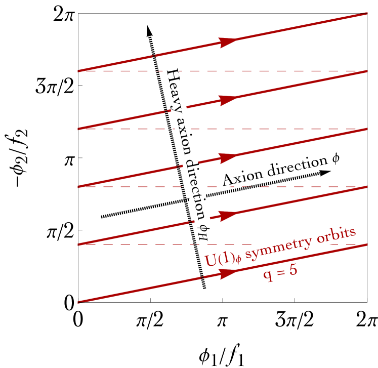
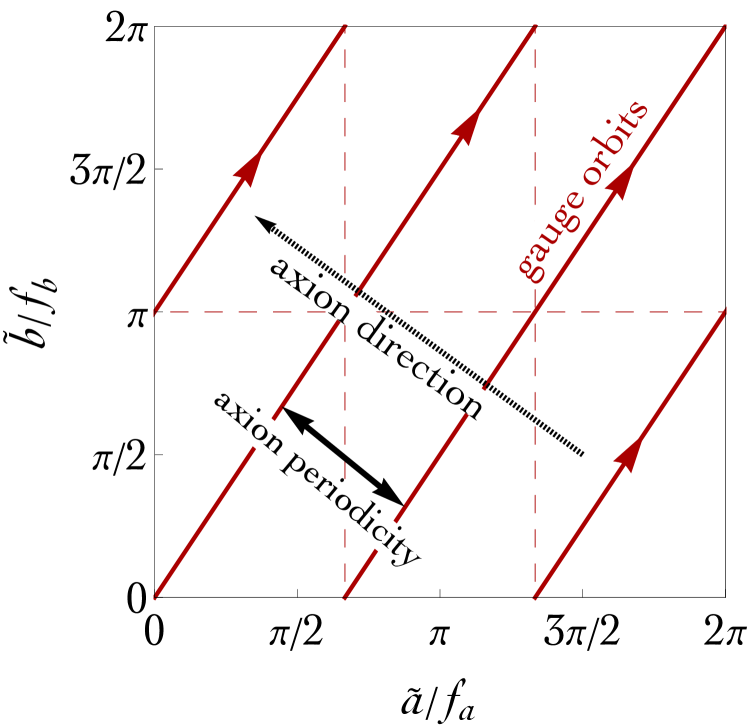
Figure 15: Left panel. The red lines follow the $U(1)_{\phi}$ orbits described by the symmetry transformation in eq. (103) with $q=5$. For illustrative purposes, we also show the direction in field space corresponding to the axion $\phi$ and the massive mode $\phi_{H}$. Right panel. The red lines follow the gauge orbits described by the symmetry transformation in eq. (94). The axion direction is orthogonal to the gauge orbits (black arrow, see section 6.3 for details).

We can visualize the periodicity of the flat direction $\phi$ by means of a simple plot, as shown in the left panel of fig. 15. Let us start from the point in field space $(\phi_{1}=0,\phi_{2}=0)$, with $\phi=0$, and follow the $U(1)_{\phi}$ orbits (solid red lines) obtained from the symmetry transformation in eq. (103) by continuously changing the parameter $c$. For illustration, we take $q=5$. Because of the periodicities $\phi_{i=1,2}\equiv\phi_{i=1,2}+2\pi f_{i=1,2}$, the $U(1)_{\phi}$ orbits are wrapped in the elementary domain $\phi_{1}/f_{1}=[0,2\pi]$, $-\phi_{2}/f_{2}=[0,2\pi]$. Notice that $\phi_{H}$ is invariant under the symmetry transformation in eq. (103), and it describes the direction orthogonal to the $U(1)_{\phi}$ orbits. The axion direction, on the contrary, is aligned with the $U(1)_{\phi}$ orbits (black arrows in fig. 15). The axion field comes back to the origin after a distance in field space

$$\Delta\phi=2\pi\sqrt{q^{2}f_{1}^{2}+f_{2}^{2}}\equiv 2\pi f_{\rm eff}~{},$$ (105)

which is enhanced by the winding number $q$ if compared with the original periodicities $2\pi f_{1}\sim 2\pi f_{2}$.

In terms of mass eigenstates, the Lagrangian density takes the simple form

$$\mathcal{L}_{\rm CW}^{(2)}=\frac{1}{2}(\partial_{\mu}\phi)(\partial^{\mu}\phi)+\frac{1}{2}(\partial_{\mu}\phi_{H})(\partial^{\mu}\phi_{H})-\frac{m_{H}^{2}}{2}\phi_{H}^{2}+\dots~{},$$ (106)

with $m_{H}^{2}$ defined by the non-zero eigenvalue in eq. (104), and where $\dots$ represents higher order in the potential for $\phi_{H}$. The massless scalar field $\phi$ corresponding to the unbroken $U(1)_{\phi}$ symmetry admits, in full analogy with the construction we put forward in section 2, wormhole solutions whose quantization condition is set by the periodicity $2\pi f_{\rm eff}$. We remark that $\phi$ represents the only direction in field space that can accommodate wormhole solutions as presented here. To understand this point one might consider wormhole solutions for the fields $\phi_{1,2}$ with decay constants $f_{1,2}\ll f_{eff}$ defined by the Lagrangian in eq. (102) and see if the potential $V(\phi_{1},\phi_{2})$ can be treated as a small perturbation. However, it is possible to see that gravitational instantons computed for the free field $\phi_{1,2}$ do not minimize the potential $V(\phi_{1},\phi_{2})$. As a consequence of the latter, instead of being a small correction, the potential gives a large contribution to the action when integrating over large scales away from the throat, and this makes these solutions, on balance, irrelevant.

This conclusion can be generalized to the case of $N+1$ axions. The Lagrangian density is

$$\mathcal{L}_{\rm CW}^{(N+1)}=\frac{1}{2}\sum_{j=0}^{N}(\partial_{\mu}\phi_{j})(\partial^{\mu}\phi_{j})+\underbrace{\sum_{j=0}^{N-1}\Lambda_{j}^{4}\cos\left(\frac{\phi_{i}}{f_{i}}+q\frac{\phi_{i+1}}{f_{i+1}}\right)}_{\equiv V(\phi_{i})}~{}.$$ (107)

The periodicity of the flat direction is given by [91, 92]

$$f_{\rm eff}=\sqrt{\sum_{i=0}^{N}\left(\prod_{j=i}^{N-1}q^{2}\right)f_{i}^{2}}\overset{f_{i=0,\dots,N}\equiv f}{=}f\sqrt{\frac{-1+(q^{2})^{N+1}}{-1+q^{2}}}\approx q^{N}f~{},$$ (108)

where in the equality we assumed for simplicity equal decay constant $f_{i=0,\dots,N}\equiv f$. As before, it is possible to construct wormhole solutions in connection with the Goldstone boson $\phi$ associated with the unbroken non-linearly realized $U(1)_{\phi}$ symmetry. The periodicity of $\phi$, $\Delta\phi=2\pi f_{\rm eff}\approx 2\pi q^{N}f$, is completely fixed by the clockwork construction, and it sets the quantization condition discussed in section 2.1.

From this discussion, it is clear that the instanton action is controlled by the ratio $M_{\rm Pl}/f_{\rm eff}$, and that non-perturbative breaking effects prevent from the possibility to have trans-Planckian field excursions: Gravity breaks explicitly the $U(1)$ direction left unbroken by the clockwork construction.

However, in order to provide a rock-solid conclusion, it is important to keep in mind – in close analogy with what discussed in section 6.1 – the possible rôle played by UV dynamics. For instance, the Lagrangian density in eq. (107) could be generated by the dynamics describing $N+1$ complex scalar fields $\Phi_{i}=[(\rho_{i}+f_{i})/\sqrt{2}]e^{\imath\phi_{i}/f_{i}}$ subject to the potential

$$\mathcal{V}(\Phi_{i})=\sum_{i=0}^{N}\left(-m_{i}^{2}|\Phi_{i}|^{2}+\frac{\lambda_{i}}{4}|\Phi_{i}|^{4}\right)+\sum_{i=0}^{N-1}\left(\epsilon_{i}\Phi_{i}^{{\dagger}}\Phi_{i+1}^{3}+h.c.\right)~{},$$ (109)

with $m_{i}\sim f_{i}$, $\lambda_{i}\sim 1$, after integrating out the radial modes. In this setup, one gets $\Lambda_{i}\equiv(\epsilon_{i}f_{i}f_{i+1}^{3}/2)^{1/4}$. The situation in similar in spirit to the setup explored in section 6.1 with the additional complication given by the presence of more fields and explicit breaking terms controlled by the order parameters $\epsilon_{i}$. The results of section 6.1 suggest that the presence of extra fields does modify the geometry of the wormhole solution. However, this could result – as explicitly proved in section 6.1 considering the presence of a dynamical radial mode – in a decrease of the wormhole action, with a consequent tightening of the amount of symmetry breaking.

Within the present study, no firm conclusion can be established. Nevertheless, we argue that the possible presence of Euclidean wormhole solutions represents the most concrete threat against the possibility to engineer trans-Planckian field excursions via the clockwork mechanism. We think this is an interesting open question, and we leave it for future investigation.

7 Wormhole solutions for a generic Goldstone coset

Let us start with a lightning review of the treatment of Goldstone bosons from the coset $\mathfrak{G}/\mathfrak{H}$ in the formalism of CCWZ [93, 94]. The broken part of the Lie algebra will be denoted by the generators $X_{A}$ whereas the un-broken symmetry generators are $T_{a}$ with the following structure

$$\left[T_{a}\,,T_{b}\right]=\imath f_{ab}^{\,\,\,\,\,c}\,T_{c}~{},~{}~{}~{}~{}~{}~{}~{}~{}~{}~{}~{}~{}~{}~{}~{}\left[T_{a}\,,X_{B}\right]=\imath f_{aB}^{\,\,\,\,\,C}\,X_{C}~{},$$ (110)

where the last equation follows for compact groups and we take the generators to be hermitian. The Goldstones parametrize the broken part of the group; one can write $\eta=\exp(iX\theta)$ with $\eta\in\mathfrak{G}/\mathfrak{H}$ in terms of $n={\rm dim}(\mathfrak{G})-{\rm dim}(\mathfrak{H})$ $\theta$ coordinates although different parametrizations are useful and often used. The transformation properties of $\eta$ are

$$\eta\to\mathbf{G}\,\eta\,\mathfrak{h}^{-1}(\eta)~{},$$ (111)

with $\mathbf{G}\in\mathfrak{G}$ and $\mathfrak{h}\in\mathfrak{H}$. This expression follows from the result that any element of the group can be factorized into a broken times an unbroken element and the composition law $\mathbf{G}\eta=\eta^{\prime}\mathfrak{h}(\eta)$. The basic building block is the Lie-dragged derivative which is a one-form $\omega$ living in the broken Lie algebra, or tangent space of the broken group manifold. Explicitly

$$\eta^{-1}d\eta=\imath\,\omega^{A}X_{A}+\imath\,V^{a}T_{a}~{},~{}~{}~{}~{}~{}~{}~{}~{}~{}~{}~{}d=dx^{\mu}\partial_{\mu}~{},$$ (112)

where $\omega^{A}=\omega^{A}_{\mu}dx^{\mu}$. In terms of the $\theta$ coordinates one has the vierbein and metric (we use the convention of summed repeated indices unless otherwise stated)

$$\omega^{A}_{\mu}=e_{i}^{A}(\theta)\partial_{\mu}\theta^{i}~{},~{}~{}~{}~{}~{}~{}~{}~{}~{}~{}~{}~{}G_{ij}(\theta)=e_{i}^{A}e_{j}^{B}\delta_{AB}~{}.$$ (113)

In order to extract the symmetry transformations in terms of the $\theta$ coordinates we make eq. (111) infinitesimal

$$\delta_{\epsilon}\eta=(i\epsilon^{a}T_{a}+i\epsilon^{A}X_{A})\eta-i\eta(\epsilon\cdot F(\eta))^{a}T_{a}~{},~{}~{}~{}~{}~{}~{}~{}~{}~{}~{}~{}~{}\eta^{-1}\delta_{\epsilon}\eta=\eta^{-1}(i\epsilon T+i\epsilon X)\eta-i(\epsilon\cdot F(\eta))^{a}T_{a}~{},$$ (114)

and we project out the non-linear piece $F(\eta)$ by restricting to broken generators only. We find

$$\eta^{-1}X_{A}\eta\big{|}_{X}=X_{B}e_{i}^{B}\xi_{A}^{i},~{}~{}~{}~{}~{}~{}~{}~{}~{}~{}~{}~{}~{}~{}~{}~{}~{}~{}~{}~{}~{}~{}~{}~{}~{}~{}\eta^{-1}T_{a}\eta\big{|}_{X}=X_{B}e_{i}^{B}\xi_{a}^{i},$$ (115)

where by $\big{|}_{X}$ we denote projection onto the broken generators. The above result yields the Killing vectors in $\theta$-space ($\delta_{\epsilon}\theta^{i}=\epsilon_{A}\xi_{A}^{i}$); there are $n$ Killing vectors $\xi_{A}$ associated to the coset and dim$(\mathfrak{H})$ Killing vectors $\xi_{a}$ for the unbroken symmetries. The transformation of the one-form $\omega^{A}$ under the unbroken part of the group is specially simple since the symmetry is linearly realized

$$\delta_{\epsilon}\omega^{A}\to\epsilon^{a}f_{aB}^{\,\,\,\,\,A}\omega^{B}~{},$$ (116)

where we have used the second relation in eq. (110). In coordinate space the Killing vectors by construction satisfy

$$\frac{\partial\xi^{k}}{\partial\theta^{i}}G_{kj}+G_{ik}\frac{\partial\xi^{k}}{\partial\theta^{j}}+\left(\xi^{k}\frac{\partial}{\partial\theta^{k}}\right)G_{ij}=0~{},$$ (117)

The Noether currents for the broken generators read

$$J^{\mu}_{A}=\sqrt{g}\,f^{2}\xi_{A}^{i}e_{i}^{B}e^{B}_{j}\partial^{\mu}\theta^{j}~{},$$ (118)

where we introduced the Goldstones decay constant $f$ and equivalent expressions apply for the unbroken currents. We note that, if a coordinate system can be found for which $\xi^{i}_{A}e^{B}_{i}=\delta^{A}_{\,\,B}$, the Noether currents read $\sqrt{g}\omega^{\mu}_{A}$ and their conservation can be written as the equation of motion for a one-form although the Bianchi identity is not satisfied in general.

We now turn to the action. By using the variational principle, one should be able to find non-trivial solutions of the equation of motion, and subsequently obtain the corresponding non-perturbative action by substituting back the solution in the original action – in parallel with what was done in section 2.1. It is often remarked how the axion gets an extra sign in its kinetic term when turning the action from Minkowski to Euclidean; here we observe that regardless of the sign, starting from the variational principle in Euclidean space yields a vanishing wormhole action, as we shall show below. This is remedied either using a three-form description – as done in section 2.1 – or introducing Lagrange multipliers [17, 103]. Since a general coset does not seemingly accept a three-form description we opt for the second option and write an action

$$\mathcal{S}_{\rm E}=\int d^{4}x\left[\sqrt{g}\left(-\frac{\mathcal{R}}{2\kappa}+\frac{f^{2}}{2}\partial_{\mu}\theta\,G\,\partial^{\mu}\theta\right)+\lambda^{A}(x)\partial_{\mu}(\sqrt{g}\,f^{2}\xi_{A}\,G\,\partial^{\mu}\theta)\right]$$ (119)

where $\kappa=8\pi G_{N}$, we have suppressed scalar indices which otherwise are summed univocally to build invariants and the Lagrange multiplier’s ($\lambda^{A}(x)$) coefficient is the divergence of the Noether currents ($J^{\mu}=\sqrt{g}f^{2}\xi G\partial^{\mu}\theta$) which vanishes on-shell. Here we have used $\theta$ coordinates yet the following derivation does not require explicit expressions for the metric $G$ or the Killing vectors; in terms of the one form $\omega$ the kinetic term of the Goldstones reads simply $\omega_{A}^{\mu}\omega_{\mu}^{A}/2$.

The variational principle yields the equations of motion $\left.\delta\mathcal{S}_{\rm E}\right|_{\delta g_{\mu\nu}}=0$, $\left.\delta\mathcal{S}_{\rm E}\right|_{\delta\theta}=0$, $\left.\delta\mathcal{S}_{\rm E}\right|_{\delta\lambda^{A}}=0$ with

$$\left.\delta\mathcal{S}_{\rm E}\right|_{\delta g_{\mu\nu}}=$$ (120)

$$\int d^{4}x\frac{\sqrt{g}}{2\kappa}\left[\mathcal{R}^{\mu\nu}-\frac{g^{\mu\nu}}{2}\mathcal{R}+\kappa f^{2}\left(\frac{g^{\mu\nu}}{2}\partial_{\rho}\theta G\partial^{\rho}\theta-\partial^{\mu}\theta G\partial^{\nu}\theta\right)-\kappa f^{2}\left(g^{\mu\nu}\partial_{\rho}\lambda\xi G\partial^{\rho}\theta-2\partial^{\mu}\lambda\xi G\partial^{\nu}\theta\right)\right]\delta g_{\mu\nu}~{},$$

$$\left.\delta\mathcal{S}_{\rm E}\right|_{\delta\theta}=$$ (121)

$$\int d^{4}x\,f^{2}\left[-\delta\theta\partial_{\mu}\left(\sqrt{g}\,G\partial^{\mu}\theta\right)+\frac{\sqrt{g}}{2}\partial_{\mu}\theta\left(\delta\theta\frac{\partial}{\partial\theta}\right)G\partial^{\mu}\theta+\delta\theta\partial_{\mu}\left(\sqrt{g}G\xi\partial^{\mu}\lambda\right)-\partial_{\mu}\lambda\left(\delta\theta\frac{\partial}{\partial\theta}\right)\xi G\partial^{\mu}\theta\right]~{},$$

$$\left.\delta\mathcal{S}_{\rm E}\right|_{\delta\lambda^{A}}=\int d^{4}x\,f^{2}\delta\lambda^{A}\partial_{\mu}\left(\sqrt{g}\,\xi_{A}G\partial^{\mu}\theta\right)~{},$$ (122)

Taking the trace in Einstein equations, if we omit $\lambda$ terms, yields $-\mathcal{R}+\kappa f^{2}\partial_{\mu}\theta G\partial^{\mu}\theta=0$ and a vanishing action (regardless of the sign that one can change with $\kappa f^{2}$). The rôle of the extra $\lambda$ term, as we shall see in the following, is exactly to turn this result into a properly defined variational principle for wormhole solutions with non-vanishing action. In this regard, our result is the generalization of the construction put forward in [17] to the case of a generic coset.

Most of the computation now involves manipulations of the equations of motion in order to put them in a clean and readable form, and we proceed as follows. In the equation for the Goldstones we perform the substitution $\delta\theta^{i}=\partial_{\nu}\lambda^{B}\xi^{i}_{B}$, and, after repeated use of the definition of Killing vectors with respect to the metric in eq. (117), we find

$$\partial_{\nu}\lambda^{B}\partial_{\mu}\left[\sqrt{g}\xi_{B}G\left(\xi\partial^{\mu}\lambda-\partial^{\mu}\theta\right)\right]+\partial_{\mu}\lambda^{A}\partial_{\nu}\lambda^{B}\left(\xi_{A}\frac{\partial\xi_{B}}{\partial\theta}-\xi_{B}\frac{\partial\xi_{A}}{\partial\theta}\right)G\partial^{\mu}\theta=0~{},$$ (123)

where the last term is antisymmetric in the summed indices $A,B$ and proportional to the structure constants. This means that, for spherically symmetric solutions which depend only on the radius $r$ as the ones we are interested in, such a term cancels, since $\partial_{r}\lambda^{A}\partial_{r}\lambda^{B}$ is symmetric in $A,B$. From now on, we focus on this type of solutions, $\theta(r)^{i}$, $\lambda^{A}(r)$, and we adopt the spherically symmetric metric in eq. (12). As remarked above eq. (123) reduces in this case to

$$\partial_{r}\lambda_{B}\partial_{r}\left[\sqrt{g}\xi_{B}G\left(\xi_{A}\partial^{r}\lambda_{A}-\partial^{r}\theta\right)\right]=0~{},$$ (124)

solved by $\xi_{A}\partial_{\mu}\lambda^{A}=\partial_{r}\theta$. On passing, we note that this substitution in Einstein equations yields $\mathcal{R}+\kappa f^{2}\partial_{r}\theta G\partial^{r}\theta=0$, and a non-zero on-shell action. This relation for $\lambda$ back into the Goldstone equation of motion eq. (121) yields, substituting $\delta\theta=\partial_{r}\theta$

$$\frac{1}{2}\sqrt{g}\partial_{r}\theta\left(\partial_{r}G\right)\partial^{r}\theta-\sqrt{g}\partial_{r}\theta(\partial_{r}G\xi)\partial^{r}\lambda=0~{}.$$ (125)

We now use the eq. (122) for the variation of the Lagrange multiplier to substitute $\partial_{r}\xi$. Eq. (125) above becomes

$$-\frac{1}{2}\sqrt{g}\partial_{r}\theta\left(\partial_{r}G\right)\partial^{r}\theta+\partial_{r}\theta(\partial_{r}\sqrt{g}G\partial^{r}\theta)=0~{},$$ (126)

and, after introducing a total derivative

$$\frac{1}{2}\partial_{r}(\partial_{r}\theta\sqrt{g}G\partial^{r}\theta)+\frac{1}{2}\partial_{r}\theta\sqrt{g}G\partial^{r}\theta\frac{g_{rr}}{\sqrt{g}}\partial_{r}\left(\frac{\sqrt{g}}{g_{rr}}\right)=0~{},$$ (127)

which can be integrated to find

$$\sqrt{g}\partial_{r}\theta G\partial^{r}\theta=C\frac{g_{rr}}{\sqrt{g}}=C\frac{\alpha}{\beta^{3}}~{},$$ (128)

where for consistency the constant $C\geq 0$. Finally, we substitute the Goldstone boson kinetic term in eq. (128) back in the Einsteins equations

$$-\frac{3\mathcal{K}\alpha^{2}}{\beta^{2}}+\frac{3(\partial_{r}\beta)^{2}}{\beta^{2}}+\frac{\kappa f^{2}}{2}C\frac{\alpha^{2}}{\beta^{6}} = 0~{},$$ (129)

$$\hat{g}_{ij}\left[-\mathcal{K}-\frac{2\beta\partial_{r}\beta\partial_{r}\alpha}{\alpha^{3}}+\left(\frac{\partial_{r}\beta}{\alpha}\right)^{2}+2\frac{\beta\partial_{r}^{2}\beta}{\alpha^{2}}\right]-\kappa f^{2}\hat{g}_{ij}\frac{\beta^{2}}{2\alpha^{2}}C\frac{\alpha^{2}}{\beta^{6}} = 0~{},$$ (130)

which, remarkably, have the same structure and solution for the metric as found in the axion case, see eqs. (14-15). The positive-definite constant $C$ can be given in terms of the $n$ Noether currents which are constants of motion $\sqrt{g}\xi_{A}G\partial^{r}\theta=C_{A}$; this in certain cases takes a simple form as the sum of the squares but a general expression for all cases is not known to us.

Let us now move to discuss the most important aspect of this computation, that is the potential that these wormhole solutions generate as a consequence of the explicit symmetry breaking that they induce. As emphasized in the discussion we put forward in the first part of this letter, the crucial point in this respect is to understand the correct quantization condition. In the simple case of the $U(1)$ symmetry, the quantization condition is related to the periodicity of the axion field. In the generalization to the coset space $\mathfrak{G}/\mathfrak{H}$, the fact that the Goldstone manifold is compact discretizes the possible charges and, as a consequence, the wormhole action. However, the discussion of the geometry a generic coset can be forbiddingly complicated. To shed light on the issue, we shall consider in the rest of this section an explicit example. In order to make an educated choice, as ever, symmetry is helpful, in particular the unbroken symmetry. In this respect the maximal unbroken symmetry allowed is $O(n)$ for $n$ Goldstones, which is the largest linearly realised symmetry that the associated tangent space, $\omega_{\mu}^{A}$, admits. A breaking pattern that yields this unbroken symmetry is $O(n+1)/O(n)$, which we will adopt as an explicit case to exemplify our discussion. One has $n$ broken generators $X_{A}$ and $n(n-1)/2$ unbroken ones $T_{a}$ that read – we will use antisymmetric generators and therefore there is no need for factors of $\imath$ in the following:

$$(X_{A})_{\alpha\beta}=\delta_{\beta}^{n+1}\delta_{\alpha}^{A}-\delta_{\alpha}^{n+1}\delta_{\beta}^{A}~{},~{}~{}~{}~{}~{}~{}~{}~{}~{}~{}~{}~{}~{}~{}(T_{a})_{\alpha\,n+1}=(T_{a})_{n+1\,\beta}=0~{},~{}{\rm with}~{}~{}T_{a}^{T}=-T_{a}~{}.$$ (131)

The Goldstone fields can be taken as $\theta^{i}$ with $i=1,..,n$ but, motivated by the symmetries of the unbroken group, we shall use in the following spherical coordinates $\theta=\rho\,u(\varphi)$, with $u\cdot u=1$. We therefore have one radius $\rho$ and $n-1$ angles $\varphi^{i}$. The Goldstone matrix reads

$$\eta=e^{X\cdot\theta}=e^{\rho X\cdot u}=\left(\begin{array}[]{cc}1-(1-\cos\rho)uu^{T}&\sin\rho\,u\\ -\sin\rho\,u^{T}&\cos\rho\end{array}\right)~{},$$ (132)

where we note that $\rho+2\pi$ gives the same group element as $\rho$. This yields the one-form

$$\eta^{-1}d\eta\big{|}_{X}=\omega^{A}X_{A}=u^{A}X_{A}d\rho+\sin\rho\frac{\partial u^{A}}{\partial\varphi^{i}}X_{A}d\varphi^{i}~{},$$ (133)

which, in turn, gives a kinetic term for the Goldstones

$$\frac{f^{2}}{2}\omega_{\mu}^{A}\omega_{A}^{\mu}=\frac{f^{2}}{2}\left(\partial_{\mu}\rho\partial^{\mu}\rho+\sin^{2}\rho\,\partial_{\mu}\varphi^{i}\frac{\partial u^{A}}{\partial\varphi^{i}}\delta_{AB}\frac{\partial u^{B}}{\partial\varphi^{j}}\partial^{\mu}\varphi^{j}\right)~{},$$ (134)

where $(\partial u/\partial\varphi)^{2}$ is the metric in a $S_{n-1}$ sphere. Using eq. (118), the Noether currents can be found to be

$$J^{\mu}_{A} = f^{2}\sqrt{g}(\xi_{A}\cdot e)^{B}\omega_{B}^{\mu}=f^{2}\sqrt{g}\left(u_{A}\partial^{\mu}\rho+\sin\rho\cos\rho\frac{\partial u_{A}}{\partial\varphi^{i}}\partial^{\mu}\varphi^{i}\right)~{},$$ (135)

$$J^{\mu}_{a} = f^{2}\sqrt{g}(\xi_{A}\cdot e)^{B}\omega_{B}^{\mu}=f^{2}\sqrt{g}\sin^{2}\rho\,u^{T}T_{a}\frac{\partial u}{\partial\varphi}\partial^{\mu}\varphi~{},$$ (136)

and in this case we can find the explicit connection between kinetic term and Noether currents by taking the sum over the unbroken currents

$$\sqrt{g}f^{2}\omega_{\mu}^{A}\omega^{\mu}_{A}=\frac{1}{\sqrt{g}f^{2}}\left(J_{\mu}^{A}J^{\mu}_{A}+J_{\mu}^{a}J^{\mu}_{a}\right)~{}.$$ (137)

We now proceed in parallel to section 2.1. We denote an instanton solution with $\bar{\rho}$ , $\bar{\varphi}$, and we consider a variation of the fields $\delta\rho$, $\delta\varphi^{i}$ around it. The first variation of the action reads, after using the equations of motion for the background:

$$\delta\mathcal{S}=\int drd\Omega_{3,1}\frac{d}{dr}\left[\sqrt{g}f^{2}\left(\delta\rho\partial^{r}\bar{\rho}+\delta\varphi^{i}\sin^{2}\bar{\rho}\frac{\partial u}{\partial\varphi^{i}}\frac{\partial u}{\partial\varphi^{j}}\partial^{r}\bar{\varphi}^{j}\right)\right]~{}.$$ (138)

If we take the variations to be independent from the solid angle $\Omega_{3}$, we can rewrite $\delta\mathcal{S}$ in terms of charges $Q_{A(a)}=\int d\Omega_{3,1}J_{A(a)}^{r}$. We find

$$\delta\mathcal{S}=\left[\delta\rho\left(\bar{u}^{A}Q_{A}\right)+\delta\varphi^{i}\left(\bar{u}\cdot T_{a}\cdot\frac{\partial\bar{u}}{\partial\varphi^{i}}Q_{a}\right)\right]~{},$$ (139)

where there is a sum over broken $Q_{A}$ and unbroken $Q_{a}$ charges. The explicit form of this expression is not relevant, what is important to note is that if gravity is to respect the unbroken symmetry, which certainly would be the case if it were gauged, the solutions would have $Q_{a}=0$ and therefore $\varphi$ coordinates would not get a potential. On the other hand the radius $\rho$ gets a contribution proportional to broken charges $Q_{A}$. Furthermore, the periodicity of this field, in full analogy with the axion case, discretizes the possible charges to be $\bar{u}^{A}Q_{A}=k$, with $k\in\mathbb{Z}$. We can expect therefore a potential generated for the radial coordinate as follows

$$V(\rho)=-Ke^{-\mathcal{S}_{\rm inst}}\cos\rho~{},$$ (140)

which nevertheless produces a mass term for all Goldstone bosons. To visualize this fact, notice that the minimum of eq. (140) sits at $\rho=0$ were the spherical coordinate system is singular. It is therefore better to go back to $\theta$ coordinates. We find

$$-V(\theta^{i})=Ke^{-\mathcal{S}_{\rm inst}}\cos\rho\simeq\frac{K}{2}e^{-\mathcal{S}_{\rm inst}}\rho^{2}=\frac{K}{2}e^{-\mathcal{S}_{\rm inst}}\sum_{i}(\theta^{i})^{2}$$ (141)

This means gravity produces a mass for all Goldstone bosons. Although obtained in the specific case of the $O(n+1)/O(n)$ symmetry breaking pattern, it is tempting to generalize this result to a general coset. We postpone the verification of this conjecture to future investigation.

8 Conclusions and outlook

The explicit breaking of global symmetries induced by gravitational effects is a mesmerising phenomenon. Furthermore, far from academic, this issue could have direct implication in phenomenology.

In this paper we considered the specific case of the global shift symmetry of a Goldstone boson, and we explored the non-perturbative breaking due to Euclidean gravitational instantons in the context of Einstein gravity (aka wormholes).

This field has been studied in a decades-long endeavour, and in this regard the main novelties of our analysis are the following.

• Theoretical analysis. On the theory side, we addressed the problem of stability of wormhole solutions by computing the spectrum of the quadratic action, and we found a positive spectrum. This result is of fundamental importance since only in the absence of negative eigenvalues the gravitational instantons mediate tunneling transitions between degenerate vacua, in parallel with other known situations both in Quantum Mechanics and Quantum Field Theory. In turn, this property allows to consistently compute the effective potential generated by gravitational instantons. The latter, as a consequence of its non-perturbative nature, is characterized by the suppression factor $e^{-\mathcal{S}_{\rm inst}}$, where $\mathcal{S}_{\rm inst}$ is the wormhole action which scales with the Goldstone decay constant and Planck mass as $\mathcal{S}_{\rm inst}\propto M_{\rm Pl}/f_{a}$.

• Phenomenological analysis. On the phenomenological side, we focused our analysis on the compelling case of the QCD axion. By computing non-perturbative gravitational corrections to the QCD axion potential, we found the following lower bound on the mass of the QCD axion

  $$m_{a}\gtrsim 4.8\times 10^{-10}\,{\rm eV}~{},~{}~{}~{}~{}f_{a}\lesssim 10^{16}\,{\rm GeV}~{}.$$ (142)

  As an application, we discussed important consequences related to black hole superradiance, and we showed that the mass range $m_{a}=[10^{-14},10^{-10}]$ eV motivated by experimental searches and phenomenological considerations is theoretically disfavored.

  In addition to the QCD axion, we discussed the case of ultralight scalars as cosmological dark matter. We showed that non-perturbative gravitational effects due to Einstein gravity generate a mass term in agreement with the estimate of the relic abundance based on the misalignment mechanism. In numbers, we found a dark matter candidate with mass $m_{a}\simeq 2.5\times 10^{-18}$ eV corresponding to the decay constant $f_{a}\simeq 8\times 10^{15}$ GeV.

  Finally, we discussed to rôle of non-perturbative gravitational corrections in connection with the relaxation of the electroweak scale and the clockwork mechanism.

We concluded with a derivation of the of wormhole solution for a generic Goldstone coset, and we inspected the breaking pattern $O(n+1)/O(n)$ to find that all Goldstone bosons in the coset acquire a mass via gravitational effects.

Appendix A Dual Formulation of broken symmetry phases

A.1 Axions and forms

Let us start considering the theory of a massless Goldstone field $\theta$ described by the Lagrangian density

$$\mathcal{L}_{\theta}=\frac{f_{a}^{2}}{2}(\partial_{\mu}\theta)(\partial^{\mu}\theta)~{}.$$ (143)

For simplicity, we restrict here to flat space. It is straightforward to check that $\mathcal{L}_{\theta}$ can be obtained from

$$\mathcal{L}_{J}=i(\partial_{\mu}\theta)J^{\mu}+\frac{1}{2f_{a}^{2}}J_{\mu}J^{\mu}~{},$$ (144)

after eliminating the non-dynamical current $J^{\mu}$ by means of its algebraic equation of motion $J^{\mu}=-if_{a}^{2}(\partial^{\mu}\theta)$. Equivalently, after integration by parts, we have

$$\mathcal{L}_{J}=-i(\partial_{\mu}J^{\mu})\theta+\frac{1}{2f_{a}^{2}}J_{\mu}J^{\mu}~{},$$ (145)

where now the Goldstone boson field is non-dynamical, implying the constraint $\partial_{\mu}J^{\mu}=0$. The Lagrangian density in eq. (143) is therefore nothing but $\mathcal{L}_{J}=J_{\mu}J^{\mu}/2f_{a}^{2}$, subject to the current conservation constraint $\partial_{\mu}J^{\mu}=0$. The latter can be formally solved by introducing the antisymmetric tensor field $B$, with $J^{\mu}\equiv-\frac{i}{2}\epsilon^{\mu\nu\rho\sigma}(\partial_{\nu}B_{\rho\sigma})$. From these simple manipulations follows that the Goldstone theory admits a description in terms of an antisymmetric tensor field. Using the condition $J^{\mu}=-if_{a}^{2}(\partial^{\mu}\theta)$, we have

$$f_{a}^{2}(\partial^{\mu}\theta)=\frac{1}{2}\epsilon^{\mu\nu\rho\sigma}(\partial_{\nu}B_{\rho\sigma})~{}~{}~{}~{}~{}\Longrightarrow~{}~{}~{}~{}~{}f_{a}^{2}\epsilon_{\mu\alpha\beta\lambda}(\partial^{\mu}\theta)=\frac{1}{2}\epsilon_{\mu\alpha\beta\lambda}\epsilon^{\mu\nu\rho\sigma}(\partial_{\nu}B_{\rho\sigma})\equiv H_{\alpha\beta\lambda}~{},$$ (146)

where $H$ is the dual strength of the antisymmetric tensor field $B$, $H_{\mu\nu\rho}=\partial_{\mu}B_{\nu\rho}+\partial_{\nu}B_{\rho\mu}+\partial_{\rho}B_{\mu\nu}$. Notice that this definition implies the Bianchi identity $\epsilon^{\mu\nu\rho\sigma}(\partial_{\rho}H_{\sigma\mu\nu})=0$.

Eq. (146), $f_{a}^{2}\epsilon_{\mu\alpha\beta\lambda}(\partial^{\mu}\theta)=H_{\alpha\beta\lambda}$, incarnates the dual description of the field $\theta$ in terms of a three-form.

Notice that at this level of the analysis we did not specify the parity transformation of the Goldstone field. On the contrary, the construction in eqs. (143-146) remains valid both for scalar and pseudo-scalar bosons. From the dual relation $2f_{a}^{2}(\partial^{\mu}\theta)=\epsilon^{\mu\nu\rho\sigma}(\partial_{\nu}B_{\rho\sigma})$, it follows that if $\theta$ is a pseudo-scalar (scalar) field, then the two-form $B_{\rho\sigma}$ is forced to transform as a tensor (pseudo-tensor). Without additional input one can not tell one option from the other, both perfectly consistent (for instance, in string-inspired situation the two-form $B_{\rho\sigma}$ can be identified with the Kalb-Ramond field that, after compactification in 4-dimensions, is an even parity tensor; having this specific dual picture in mind, the field $\theta$ transforms as a pseudo-scalar).

In the dual picture, the free Lagrangian density in eq. (145) takes the form

$$\mathcal{L}_{J}=\frac{1}{4f_{a}^{2}}\left(\partial_{\nu}B_{\rho\sigma}\right)\left(\partial^{\nu}B^{\rho\sigma}\right)-\frac{1}{2f_{a}^{2}}\left(\partial^{\sigma}B_{\sigma\rho}\right)\left(\partial_{\nu}B^{\nu\rho}\right)~{}.$$ (147)

The antisymmetric tensor $B_{\rho\sigma}$ has $6$ independent components, but the gauge symmetry

$$\delta B_{\rho\sigma}=\partial_{[\rho}\Lambda_{\sigma]}=\frac{1}{2}\left(\partial_{\rho}\Lambda_{\sigma}-\partial_{\sigma}\Lambda_{\rho}\right)~{},$$ (148)

with the extra redundancy $\Lambda^{\prime}_{\sigma}=\Lambda_{\sigma}+\partial_{\sigma}\lambda$ correctly reduces to one the number of dynamical degrees of freedom.

A.2 From Minkowski to Euclidean space

Let us consider the action in curved space-time, with flat metric $\eta_{\mu\nu}={\rm diag}(+1,-1,-1,-1)$

$$\mathcal{S}=\int d^{4}x\sqrt{-g}\left[\frac{M_{\rm Pl}^{2}}{16\pi}\,\mathcal{R}+\frac{f_{a}^{2}}{2}(\partial_{\rho}\theta)(\partial^{\rho}\theta)\right]~{},$$ (149)

describing a massless Goldstone boson field $\theta$ minimally coupled to Einstein gravity. As discussed in section 2.1, the field $\theta$ admits a dual description in terms of an antisymmetric two-form with field strength $H_{\mu\nu\rho}$ given by $H_{\mu\nu\rho}=f_{a}^{2}\epsilon_{\mu\nu\rho\sigma}\left(\partial^{\sigma}\theta\right)$. In Lorentzian space-time, we have the following identity

$$\frac{f_{a}^{2}}{2}(\partial_{\rho}\theta)(\partial^{\rho}\theta)=-\frac{\mathcal{F}}{2}H_{\mu\nu\rho}H^{\mu\nu\rho}~{},$$ (150)

with $\mathcal{F}$ defined right below eq. (5). The minus sign follows from the Levi-Civita contraction $\epsilon_{\mu\nu\rho\sigma}\epsilon^{\mu\nu\rho\lambda}=(-1)^{t}\,3!\,\delta_{\sigma}^{\lambda}$, with $t=1$ in Minkowski space-time. The action in eq. (149) takes the form

$$\mathcal{S}=\int d^{4}x\sqrt{-g}\left[\frac{M_{\rm Pl}^{2}}{16\pi}\,\mathcal{R}-\frac{\mathcal{F}}{2}H_{\mu\nu\rho}H^{\mu\nu\rho}\right]~{}.$$ (151)

We are now ready to go from Minkowski – with coordinates $x\equiv(t,\vec{x})$, and metric $g_{\mu\nu}(x)$ – to Euclidean space-time – with coordinates $\tilde{x}\equiv(t_{\rm E},\vec{x})$, and metric $\tilde{g}_{\mu\nu}(\tilde{x})$ – by means of the Wick rotation $t_{\rm E}\equiv\imath t$. The Euclidean action is related to eq. (149) via $S_{\rm E}\equiv-\imath\left.\mathcal{S}\right|_{t=-\imath t_{\rm E}}$. The analytical continuation can be seen as the coordinate transformation $x\equiv(t,\vec{x})\to\tilde{x}\equiv(t_{\rm E},\vec{x})=(\lambda t,\vec{x})$, with $\lambda=\imath$. We can therefore write the general coordinate transformation

$$g_{\alpha\beta}(x)=\tilde{g}_{\mu\nu}(\tilde{x})\frac{\partial\tilde{x}^{\mu}}{\partial x^{\alpha}}\frac{\partial\tilde{x}^{\nu}}{\partial x^{\beta}}=\left(\begin{array}[]{cccc}\lambda^{2}\tilde{g}_{00}&\lambda\tilde{g}_{01}&\lambda\tilde{g}_{02}&\lambda\tilde{g}_{03}\\ \lambda\tilde{g}_{01}&\tilde{g}_{11}&\tilde{g}_{12}&\tilde{g}_{13}\\ \lambda\tilde{g}_{02}&\tilde{g}_{12}&\tilde{g}_{22}&\tilde{g}_{23}\\ \lambda\tilde{g}_{03}&\tilde{g}_{13}&\tilde{g}_{23}&\tilde{g}_{33}\end{array}\right)~{},$$ (152)

from which it follows that $g=\lambda^{2}\tilde{g}=-\tilde{g}$, and $d^{4}x\sqrt{-g}=d^{4}\tilde{x}\sqrt{\tilde{g}}(-\imath)$. The Euclidean version of eq. (151) is

$$\mathcal{S}_{\rm E}=\int d^{4}x\sqrt{\tilde{g}}\left[-\frac{M_{\rm Pl}^{2}}{16\pi}\,\mathcal{R}+\frac{\mathcal{F}}{2}H_{\mu\nu\rho}H^{\mu\nu\rho}\right]~{},$$ (153)

which coincides, after renaming $\tilde{g}$, with eq. (5). In Euclidean space, the duality relation in eq. (150) reads

$$\frac{f_{a}^{2}}{2}(\partial_{\rho}\theta)(\partial^{\rho}\theta)=\frac{\mathcal{F}}{2}H_{\mu\nu\rho}H^{\mu\nu\rho}~{},$$ (154)

where we now used $\epsilon_{\mu\nu\rho\sigma}\epsilon^{\mu\nu\rho\lambda}=(-1)^{t}\,3!\,\delta_{\sigma}^{\lambda}$, with $t=0$ in Euclidean space-time. Consequently, we reconstruct the Euclidean action in eq. (8).

Notice that it is crucial to define the Euclidean action by analytical continuation of eq. (151) rather then eq. (149). Indeed, the analytical continuation of eq. (149) would generate the Euclidean action

$$\mathcal{S}_{\rm E}=\int d^{4}x\sqrt{g}\left[-\frac{M_{\rm Pl}^{2}}{16\pi}\,\mathcal{R}-\frac{f_{a}^{2}}{2}(\partial_{\rho}\theta)(\partial^{\rho}\theta)\right]~{},$$ (155)

that features the ‘wrong’ minus sign in front of the Goldstone kinetic term.

Finally, we stress again that the construction we put forward in this appendix, as well as the consequent wormhole solutions, does not rely on the transformation properties under parity of the Goldstone boson. This suggests that wormhole solutions can be defined for both free massless scalar and pseudo-scalar fields.

A.3 Axion charge quantization

In this appendix we provide a more quantitative picture of the quantization condition discussed at the end of section 2.1. To this end, we exploit the analogy with the quantization of the electric charge in the presence of a magnetic monopole.

The magnetic field of a putative magnetic monopole placed at the origin of $\mathbb{R}^{3}$ is

$$\vec{\mathcal{B}}(\vec{r})=\frac{g_{\rm M}}{4\pi}\frac{\vec{r}}{r^{3}}~{},~{}~{}~{}~{}~{}~{}~{}g_{\rm M}=\int_{S_{2}}\vec{\mathcal{B}}\cdot d\vec{S}~{},$$ (156)

where in the second equation the magnetic charge $g_{\rm M}$ corresponds to the magnetic flux through the sphere $S_{2}$. Bearing in mind the relation with the electromagnetic field strength, $F_{ij}=-\epsilon_{ijk}\mathcal{B}_{k}$, one can already identify the analogy with the three-form field $H_{ijk}=\epsilon_{ijk}\mathcal{H}_{0}=\epsilon_{ijk}n/2\pi^{2}r^{3}$ and the computation of the flux in eq. (18). Of course, in the electromagnetic case we are dealing with a two-form field strength $F_{\mu\nu}=\partial_{\mu}A_{\nu}-\partial_{\nu}A_{\mu}$ while in the axion case the field strength is the three-form $H_{\mu\nu\rho}=\partial_{\mu}B_{\nu\rho}+\partial_{\nu}B_{\rho\mu}+\partial_{\rho}B_{\mu\nu}$ but the comparison is evident. The rôle of the electromagnetic potential $A_{\mu}$ is played by the antisymmetric tensor $B_{\mu\nu}$. The obstacle is that it is not possible to find a vector potential such that $\vec{\nabla}\times\vec{A}=\vec{\mathcal{B}}$ since the monopole field is not divergenceless. The best that one can do is to define (in ordinary spherical coordinates) the vector potentials

$$\vec{A}_{1}\equiv\frac{g_{\rm M}(1-\cos\theta)}{4\pi r\sin\theta}\hat{\phi}~{},~{}~{}~{}~{}~{}~{}~{}\vec{A}_{2}\equiv-\frac{g_{\rm M}(1+\cos\theta)}{4\pi r\sin\theta}\hat{\phi}~{},$$ (157)

defined, respectively, in $R_{1}:\theta\in[0,\pi/2+\delta)$ and $R_{2}:\theta\in(\pi/2-\delta,\pi]$ with an overlap region $\pi/2-\delta<\theta<\pi/2+\delta$. In their domains, both potentials satisfy $\vec{\nabla}\times\vec{A}_{1,2}=\vec{\mathcal{B}}$ but they are singular in the complementary region. This is the same ambiguity one encounters for the two-form potential $B$ in the axion case. The only way to obtain a consistent picture is to show that the two vector potentials describe the same physics in the overlap region. Said differently, $\vec{A}_{1}$ and $\vec{A}_{2}$ must be related by a gauge transformation $\vec{A}\to\vec{A}^{\prime}=\vec{A}+\vec{\nabla}\chi$. From $\vec{A}_{1}-\vec{A}_{2}=\vec{\nabla}\chi$ one immediately finds $\chi\equiv g_{\rm M}\phi/2\pi$. Notice that the function $\chi(\phi)$ is not continuous since the azimuthal angle is defined modulo $2\pi$. This is actually crucial for the existence of a non-zero flux in eq. (156) since

$$g_{\rm M}=\int_{S_{2}}\vec{\mathcal{B}}\cdot d\vec{S}=\int_{R_{1}}(\vec{\nabla}\times\vec{A}_{1})\cdot d\vec{S}+\int_{R_{2}}(\vec{\nabla}\times\vec{A}_{2})\cdot d\vec{S}=\int_{0}^{2\pi}(\partial\chi/\partial\phi)d\phi=\chi(2\pi)-\chi(0)~{}.$$ (158)

Dirac quantization proceeds as follows. We consider a test particle of mass $m$ and charge $q$ in the field of the magnetic monopole. Its wavefunction satisfies the Schrödinger equation $-\not{h}^{2}/2m(\vec{\nabla}+\imath e\vec{A})^{2}\psi=\imath\not{h}\partial\psi/\partial t$, with $e=q/\not{h}$, and the gauge transformation $\vec{A}\to\vec{A}^{\prime}=\vec{A}+\vec{\nabla}\chi$ transforms $\psi$ into $\psi^{\prime}=e^{-\imath e\chi}\psi=e^{-\imath eg_{\rm M}\phi/2\pi}\psi$. Since $\phi=0$ and $\phi=2\pi$ are the same physical point, consistency of Quantum Mechanics requires the wavefunction $\psi^{\prime}$ to be single valued. The quantization condition $eg_{\rm M}=2\pi k$, with $k\in\mathbb{Z}$, then follows.

Dirac quantization involves the product $eg_{\rm M}$ of electric and magnetic charge. The electric charge of a particle is given by the surface integral at spatial infinity over a $S_{2}$ sphere of the Hodge dual of the electromagnetic field strength two-form $F_{\mu\nu}$. Conversely, the magnetic charge of a particle is given by the surface integral at spatial infinity over a sphere $S_{2}$ of the electromagnetic field strength two-form $F_{\mu\nu}$, as already discussed in eq. (156).

The quantization in the axion case is based on the fact that potentials of higher rank admit the following generalization. Formally, in $D$ dimensions, the ‘electric’ charge $Q_{\rm E}$ is the integral over the sphere $S_{D-(p+2)}$ of the Hodge dual of the $(p+2)$-form field strength. For the axion three-form $H$, $p=1$, and in $D=4$ dimensions $Q_{\rm E}=\int_{S_{1}}{{}^{*}H}$. The ‘magnetic’ charge, as already noticed, is $Q_{\rm M}=\int_{S_{3}}H=n$ (see eq. (18)), that in our case corresponds to the axion charge flowing through the wormhole throat. Dirac quantization therefore generalizes to $Q_{\rm E}n=2\pi k$. If $Q_{\rm E}\neq 0$, the quantization of $n$ trivially follows. In terms of the Goldstone field, we have $Q_{\rm E}=\int_{S_{1}}{{}^{*}H}=\int_{S_{1}}d\theta$. The key observation is that this integral encompasses a closed path. This means that $Q_{\rm E}$ can be different from zero only if $\theta$ is multi-valued, and this is exactly the case for the Goldstone field since it is a phase, and possesses the periodicity $\theta=\theta+2\pi$. This concludes the argument, and shows the fundamental importance of the periodicity of the Goldstone boson field for the quantization of the axion charge along the wormhole throat.

Appendix B The Pöschl-Teller potential

We want to solve the spectral problem for the differential operator

$$\left[-\frac{d^{2}}{d\tau^{2}}+1-\frac{15}{\cosh^{2}(2\tau)}\right]u(\tau)=\lambda u(\tau)~{},$$ (159)

or, equivalently

$$\left[-\frac{d^{2}}{dx^{2}}-\frac{15/4}{\cosh^{2}x}\right]u(x)=2Eu(x)~{},~{}~{}~{}~{}{\rm with}~{}~{}2E=\left(\frac{\lambda-1}{4}\right)~{}.$$ (160)

Eq. (160) is describes the one-dimensional motion of a particle in the Pöschl-Teller potential [106]. In full generality, the dynamics in the Pöschl-Teller potential is described by the differential equation $-u^{\prime\prime}(x)-\frac{\alpha^{2}\xi(\xi-1)}{\cosh^{2}(\alpha x)}u(x)=2Eu(x)$. Eq. (160) corresponds to $\alpha=1$, $\xi=5/2$. By changing variable $y\equiv\cosh^{2}x$ we find

$$y(1-y)u^{\prime\prime}(y)+\left(\frac{1}{2}-y\right)u^{\prime}(y)-\left(\frac{15}{16y}+\frac{E}{2}\right)u(y)=0~{}.$$ (161)

After the rescaling $u(y)=y^{5/4}v(y)$ the problem reduces to the hypergeometric differential equation

$$y(1-y)v^{\prime\prime}(y)+v^{\prime}(y)\left[\xi+\frac{1}{2}-y(\xi+1)\right]-\frac{v(y)}{4}\left(\xi^{2}+2E\right)=0~{},$$ (162)

with $\xi=5/2$. We have the general solution

$$u(x)=y^{\xi/2}\left[B\sqrt{1-y}~{}_{2}F_{1}\left(a+\frac{1}{2},b+\frac{1}{2};\frac{3}{2};1-y\right)+A~{}_{2}F_{1}\left(a,b;\frac{1}{2};1-y\right)\right]~{},$$ (163)

where ${}_{2}F_{1}(a,b;c;z)$ is the Gaussian or ordinary hypergeometric function, and we introduced the short-hand notation

$$a\equiv\frac{1}{2}\left(\xi+\imath\sqrt{2E}\right)~{},~{}~{}~{}~{}~{}b\equiv\frac{1}{2}\left(\xi-\imath\sqrt{2E}\right)~{}.$$ (164)

We can separate the two independent solutions. If $B=0$, $A=1$, we have the even solution

$$u_{\rm even}(x)=\cosh^{\xi}x~{}_{2}F_{1}\left(a,b;\frac{1}{2};-\sinh^{2}x\right)~{}.$$ (165)

If $A=0$, $B=\imath$ we have the odd solution

$$u_{\rm odd}(x)=\cosh^{\xi}x\sinh x~{}_{2}F_{1}\left(a+\frac{1}{2},b+\frac{1}{2};\frac{3}{2};-\sinh^{2}x\right)~{}.$$ (166)

In order to identify the bound states with negative energy solutions, we need to study the asymptotic behavior. Using the trigonometric definitions $\sinh x=(e^{x}-e^{-x})/2$, $\cosh x=(e^{x}+e^{-x})/2$ we find

$$u_{\rm even}(x) \overset{x\to\pm\infty}{\rightarrow} \sqrt{\pi}\left[\frac{2^{2a-\xi}e^{-\imath\sqrt{2E}|x|}\Gamma(-a+b)}{\Gamma(1/2-a)\Gamma(b)}+\frac{2^{2b-\xi}e^{\imath\sqrt{2E}|x|}\Gamma(a-b)}{\Gamma(a)\Gamma(1/2-b)}\right]~{},$$ (167)

$$u_{\rm odd}(x) \overset{x\to\pm\infty}{\rightarrow} \pm\sqrt{\pi}\left[\frac{2^{2a-(\xi+1)}e^{-\imath\sqrt{2E}|x|}\Gamma(-a+b)}{\Gamma(1-a)\Gamma(1/2+b)}+\frac{2^{2b-(\xi+1)}e^{\imath\sqrt{2E}|x|}\Gamma(a-b)}{\Gamma(1/2+a)\Gamma(1-b)}\right]~{}.$$ (168)

In the presence of negative energy states, we have

$$e^{-\imath\sqrt{2E}}=e^{+\sqrt{2|E|}}~{},~{}~{}~{}~{}~{}e^{\imath\sqrt{2E}}=e^{-\sqrt{2|E|}}~{}.$$ (169)

The coefficient of $e^{-\imath\sqrt{2E}}$ must therefore vanish in order to ensure the correct asymptotic behavior. This condition leads to quantization of energy. The Gamma function diverges for negative integer numbers, and we can impose this condition to cancel the coefficient of $e^{-\imath\sqrt{2E}}$ in both $u_{\rm even}(x)$ and $u_{\rm odd}(x)$. For the even functions we find

$$\frac{1}{2}-a=-m~{}~{}~{}~{}\Longrightarrow~{}~{}~{}~{}2E_{m}^{\rm(even)}=-(-2m-1+\xi)^{2}~{},$$ (170)

whereas for the even functions we find

$$1-a=-m~{}~{}~{}~{}\Longrightarrow~{}~{}~{}~{}2E_{m}^{\rm(odd)}=-(-2m-2+\xi)^{2}~{},$$ (171)

with $m=0,1,2,\dots$.

With $\xi=5/2$ we only have one negative (even) state with energy $2E_{0}^{\rm(even)}=-9/4$ or, equivalently, $\lambda=-8$. Next, we have two states with $\lambda=0$ corresponding to $2E_{1}^{\rm(even)}=-1/4$ and $2E_{0}^{\rm(odd)}=-1/4$. Using eqs. (165,166), we find

$${\rm Odd\,eigenfunction:}~{}~{} \left\{u_{\rm odd}^{\lambda=0}(\tau)=\frac{\sinh(2\tau)}{\cosh^{3/2}(2\tau)}\right\}~{},$$ (172)

$${\rm Even\,eigenfunctions:}~{}~{} \left\{u_{\rm even}^{\lambda=-8}(\tau)=\frac{1}{\cosh^{3/2}(2\tau)}~{},~{}~{}u_{\rm even}^{\lambda=0}(\tau)=\frac{3-\cosh(4\tau)}{2\cosh^{3/2}(2\tau)}\right\}~{}.$$ (173)

The eigenfunction $u_{\rm even}^{\lambda=0}(\tau)$ is not square-integrable.

Appendix C Spectrum of tensor and inhomogeneous scalar perturbations

In this appendix we compute the spectrum of tensor and inhomogeneous scalar perturbations of the quadratic action expanded around the wormhole background.

C.1 Tensor perturbations

We exploit the results of [33] in which tensor fluctuations around instanton background were studied. The perturbed line element, in Euclidean space, is $ds^{2}=a^{2}(\tau)\left[d\tau^{2}+(\gamma_{ij}+t_{ij})dx^{i}dx^{j}\right]$, where $\gamma_{ij}$ is the background metric on the three-sphere and $a(\tau)$ the background conformal factor. As discussed in section 3.1, $t_{ij}$ is a transverse trace-free symmetric tensor. The Euclidean quadratic action takes the form [33]

$$\left.\delta\mathcal{S}_{\rm E}^{(2)}\right|_{\rm tensor}=\frac{1}{8\kappa}\int d\tau d^{3}\vec{x}\sqrt{\gamma}a^{2}\left(t^{\prime\,ij}t^{\prime}_{ij}+\nabla^{i}t^{jk}\nabla_{i}t_{jk}+2t^{ij}t_{ij}\right)~{},$$ (174)

where covariant derivatives and contractions are defined w.r.t. the metric $\gamma$. By introducing the rescaling $\tilde{t}_{ij}\equiv at_{ij}$, and integrating by parts, one finds [33]

$$\left.\delta\mathcal{S}_{\rm E}^{(2)}\right|_{\rm tensor}=\frac{1}{8\kappa}\int d\tau d^{3}\vec{x}\sqrt{\gamma}\left[\tilde{t}_{ij}\left(\hat{K}+3-\Delta\right)\tilde{t}^{ij}-\frac{d}{d\tau}\left(\frac{a^{\prime}}{a}\tilde{t}_{ij}\tilde{t}^{ij}\right)\right]~{},$$ (175)

with the Schrödinger-type operator

$$\hat{K}\equiv-\frac{d^{2}}{d\tau^{2}}+\frac{a^{\prime\prime}}{a}-1=-\frac{d^{2}}{d\tau^{2}}+\frac{1}{\cosh^{2}(2\tau)}~{},$$ (176)

where in the last step we substituted the wormhole background solution. Notice that the quadratic action in eq. (175) does not present the conformal factor problem. This is indeed correct since, as reviewed in section 3.1, the quadratic action for the trace-free part of the tensor fluctuations is not unbounded from below. The differential operator $\hat{K}$ acts on the $\tau$ variable while the Laplacian operator $\Delta$ acts on the three-dimensional space. We can therefore diagonalize them independently and add their spectra. The differential operator $\hat{K}$ does not possess negative eigenvalues since the potential is a positive function and there are no bound states. The tensor harmonics $(G_{ij})^{n}_{lm}(\psi,\phi,\varphi)$ are tensor eigenfucntions of the Laplacian operator on $S_{3}$. They satisfy the eigenvalue equation $\Delta(G_{ij})^{n}_{lm}=-(n^{2}-3)(G_{ij})^{n}_{lm}$, with $n=3,4,5,\dots$, supported by the transverse and traceless conditions $\nabla^{i}(G_{ij})^{n}_{lm}=0$ and $(G_{i}^{i})^{n}_{lm}=0$. Because of the degeneracy in $l$ and $m$, the most general solution of the eigenvalue equation is $G_{ij}^{(n)}(\psi,\phi,\varphi)=\sum_{l=2}^{n-1}\sum_{m=-l}^{l}C_{lm}^{(n)}(G_{ij})^{n}_{lm}(\psi,\phi,\varphi)$, with $C_{lm}^{(n)}$ arbitrary constants. From this general discussion it follows that the tensor Laplacian $-\Delta$ in eq. (175) has positive eigenvalues, starting from $\lambda=6$. We conclude that tensor fluctuations around the wormhole background have a positive spectrum.

C.2 Inhomogeneous scalar perturbations

We now move to discuss inhomogeneous scalar perturbations. In section 3.1 we focused on scalar homogeneous perturbations. A separated analysis is required since, as well known [34, 35], inhomogeneous perturbations have positive Euclidean action and do not suffer from the conformal factor problem. We exploit the results of [35]. In the Euclidean space, the quadratic action takes in form

$$\left.\delta\mathcal{S}_{\rm E}^{(2)}\right|_{\Delta\neq 0}=\frac{1}{2}\int d\tau d^{3}\vec{x}\sqrt{\gamma}\left\{\left(-\Delta+3\right)q\left(\hat{O}-\Delta+3\right)q+\left(-\Delta+3\right)\frac{d}{d\tau}\left[qq^{\prime}+\left(-\frac{\kappa\phi^{\prime\,2}}{4a^{\prime}/a}+\frac{\phi^{\prime\prime}}{\phi^{\prime}}\right)q^{2}\right]\right\}~{},$$ (177)

with the Schrödinger-type operator

$$\hat{O}\equiv-\frac{d^{2}}{d\tau^{2}}-\frac{\kappa\phi^{\prime\,2}}{2}+\phi^{\prime}\left(\frac{1}{\phi^{\prime}}\right)^{\prime\prime}=-\frac{d^{2}}{d\tau^{2}}+4-\frac{3}{\cosh^{2}(2\tau)}~{}.$$ (178)

As before, the differential operator $\hat{O}$ acts on the $\tau$ variable while the Laplacian operator $\Delta$ acts on the three-dimensional space. We can therefore diagonalize them independently and add their spectra. Furthermore, we already know that $-\Delta$ has positive eigenvalues starting from $\lambda=3$ (ignoring the homogeneous mode). In eq. (177) $q$ is the only physical dynamical variable describing scalar perturbations after gauge degrees of freedom are removed [35]. By defining $2\tau\equiv x$, the differential equation $\hat{O}u(\tau)=\lambda u(\tau)$ in eq. (178) takes the form

$$\left[-\frac{d^{2}}{dx^{2}}-\frac{3/4}{\cosh^{2}x}\right]u(x)=2Eu(x)~{},~{}~{}~{}~{}{\rm with}~{}~{}2E=\left(\frac{\lambda}{4}-1\right)~{}.$$ (179)

This is again a Pöschl-Teller potential with $\alpha=1$, $\xi=3/2$. We can repeat the analysis presented in appendix B. With $\xi=3/2$, we have a double-degenerate negative eigenvalue $E_{0}^{\rm even/odd}=-1/4$ but it corresponds to the positive value $\lambda=3$, that is the starting point of the spectrum of the differential operator $\hat{O}$. We therefore conclude that the spectrum of the bulk operator in eq. (177) is fully positive.

References

- [1] T. Banks, L. J. Dixon, D. Friedan and E. J. Martinec, “Phenomenology and Conformal Field Theory Or Can String Theory Predict the Weak Mixing Angle?,” Nucl. Phys. B 299, 613 (1988).
- [2] E. Witten, “Anti-de Sitter space and holography,” Adv. Theor. Math. Phys. 2, 253 (1998) [hep-th/9802150].
- [3] M. Kamionkowski and J. March-Russell, “Planck scale physics and the Peccei-Quinn mechanism,” Phys. Lett. B 282, 137 (1992) [hep-th/9202003].
- [4] S. M. Barr and D. Seckel, “Planck scale corrections to axion models,” Phys. Rev. D 46, 539 (1992).
- [5] K. S. Babu, I. Gogoladze and K. Wang, “Stabilizing the axion by discrete gauge symmetries,” Phys. Lett. B 560, 214 (2003) [hep-ph/0212339].
- [6] R. Holman, S. D. H. Hsu, T. W. Kephart, E. W. Kolb, R. Watkins and L. M. Widrow, “Solutions to the strong CP problem in a world with gravity,” Phys. Lett. B 282, 132 (1992) [hep-ph/9203206].
- [7] L. Di Luzio, E. Nardi and L. Ubaldi, “Accidental Peccei-Quinn symmetry protected to arbitrary order,” arXiv:1704.01122 [hep-ph].
- [8] H. Fukuda, M. Ibe, M. Suzuki and T. T. Yanagida, “A ‘Gauged’ Peccei-Quinn Symmetry,” arXiv:1703.01112 [hep-ph].
- [9] J. E. Kim, “Invisible Axion and Neutrino Oscillation in SU(11),” Phys. Rev. D 24, 3007 (1981).
- [10] H. M. Georgi, L. J. Hall and M. B. Wise, “Grand Unified Models With an Automatic Peccei-Quinn Symmetry,” Nucl. Phys. B 192, 409 (1981).
- [11] K. Harigaya, M. Ibe, K. Schmitz and T. T. Yanagida, “Peccei-Quinn symmetry from a gauged discrete R symmetry,” Phys. Rev. D 88, no. 7, 075022 (2013) [arXiv:1308.1227 [hep-ph]].
- [12] A. G. Dias, V. Pleitez and M. D. Tonasse, “Naturally light invisible axion in models with large local discrete symmetries,” Phys. Rev. D 67, 095008 (2003) [hep-ph/0211107].
- [13] A. G. Dias, A. C. B. Machado, C. C. Nishi, A. Ringwald and P. Vaudrevange, “The Quest for an Intermediate-Scale Accidental Axion and Further ALPs,” JHEP 1406, 037 (2014) [arXiv:1403.5760 [hep-ph]].
- [14] J. E. Kim and D. J. E. Marsh, “An ultralight pseudoscalar boson,” Phys. Rev. D 93, no. 2, 025027 (2016) [arXiv:1510.01701 [hep-ph]].
- [15] R. Kallosh, A. D. Linde, D. A. Linde and L. Susskind, “Gravity and global symmetries,” Phys. Rev. D 52, 912 (1995) [hep-th/9502069].
- [16] S. B. Giddings and A. Strominger, “Axion Induced Topology Change in Quantum Gravity and String Theory,” Nucl. Phys. B 306, 890 (1988).
- [17] K. M. Lee, “Wormholes and Goldstone Bosons,” Phys. Rev. Lett. 61, 263 (1988).
- [18] A. Hebecker, P. Mangat, S. Theisen and L. T. Witkowski, “Can Gravitational Instantons Really Constrain Axion Inflation?,” JHEP 1702 (2017) 097 [arXiv:1607.06814 [hep-th]].
- [19] M. Montero, A. M. Uranga and I. Valenzuela, “Transplanckian axions!?,” JHEP 1508, 032 (2015) [arXiv:1503.03886 [hep-th]].
- [20] T. C. Bachlechner, C. Long and L. McAllister, “Planckian Axions and the Weak Gravity Conjecture,” JHEP 1601, 091 (2016) [arXiv:1503.07853 [hep-th]].
- [21] N. Arkani-Hamed, L. Motl, A. Nicolis and C. Vafa, “The String landscape, black holes and gravity as the weakest force,” JHEP 0706, 060 (2007) [hep-th/0601001].
- [22] S. Coleman, “Aspects of symmetry - Selected Erice lectures,” Cambridge University Press (2010), book DOI.
- [23] A. I. Vainshtein, V. I. Zakharov, V. A. Novikov and M. A. Shifman, “ABC’s of Instantons,” Sov. Phys. Usp. 25, 195 (1982) [Usp. Fiz. Nauk 136, 553 (1982)].
- [24] T. Ortin, “Gravity and Strings,” Cambridge University Press.
- [25] E. Witten, “Nonabelian Bosonization in Two-Dimensions,” Commun. Math. Phys. 92 (1984) 455.
- [26] C. G. Callan, Jr., J. A. Harvey and A. Strominger, “Supersymmetric string solitons,” In Trieste 1991, Proceedings, String theory and quantum gravity ‘91 [hep-th/9112030].
- [27] R. Rohm and E. Witten, “The Antisymmetric Tensor Field in Superstring Theory,” Annals Phys. 170, 454 (1986).
- [28] T. J. Allen, “Duality and the vacuum,” Nucl. Phys. B 395, 185 (1993).
- [29] J. W. York, Jr., “Gravitational degrees of freedom and the initial-value problem,” Phys. Rev. Lett. 26, 1656 (1971).
- [30] J. W. York, Jr., “Role of conformal three geometry in the dynamics of gravitation,” Phys. Rev. Lett. 28, 1082 (1972).
- [31] G. W. Gibbons and S. W. Hawking, “Action Integrals and Partition Functions in Quantum Gravity,” Phys. Rev. D 15, 2752 (1977).
- [32] J. Garriga, X. Montes, M. Sasaki and T. Tanaka, “Canonical quantization of cosmological perturbations in the one-bubble open universe,” Nucl. Phys. B 513, 343 (1998) Erratum: [Nucl. Phys. B 551, 511 (1999)] [astro-ph/9706229].
- [33] T. Hertog and N. Turok, “Gravity waves from instantons,” Phys. Rev. D 62, 083514 (2000) [astro-ph/9903075].
- [34] S. Gratton and N. Turok, “Homogeneous modes of cosmological instantons,” Phys. Rev. D 63, 123514 (2001) [hep-th/0008235].
- [35] S. Gratton and N. Turok, “Cosmological perturbations from the no boundary Euclidean path integral,” Phys. Rev. D 60, 123507 (1999) [astro-ph/9902265].
- [36] V. A. Rubakov and O. Y. Shvedov, “A Negative mode about Euclidean wormhole,” Phys. Lett. B 383, 258 (1996) [gr-qc/9604038].
- [37] G. W. Gibbons, S. W. Hawking and M. J. Perry, “Path Integrals and the Indefiniteness of the Gravitational Action,” Nucl. Phys. B 138, 141 (1978).
- [38] P. O. Mazur and E. Mottola, “The Gravitational Measure, Solution of the Conformal Factor Problem and Stability of the Ground State of Quantum Gravity,” Nucl. Phys. B 341, 187 (1990).
- [39] S. J. Rey, “The Axion Dynamics in Wormhole Background,” Phys. Rev. D 39, 3185 (1989).
- [40] S. B. Giddings and A. Strominger, “Loss of Incoherence and Determination of Coupling Constants in Quantum Gravity,” Nucl. Phys. B 307, 854 (1988).
- [41] S. R. Coleman, “Black Holes as Red Herrings: Topological Fluctuations and the Loss of Quantum Coherence,” Nucl. Phys. B 307, 867 (1988).
- [42] J. Preskill, “Wormholes in Space-time and the Constants of Nature,” Nucl. Phys. B 323, 141 (1989).
- [43] S. W. Hawking, “The Effective action for wormholes,” Nucl. Phys. B 363, 117 (1991).
- [44] S. W. Hawking, “Wormholes in Space-Time,” Phys. Rev. D 37, 904 (1988).
- [45] S. R. Coleman, “Why There Is Nothing Rather Than Something: A Theory of the Cosmological Constant,” Nucl. Phys. B 310, 643 (1988).
- [46] I. R. Klebanov, L. Susskind and T. Banks, “Wormholes and the Cosmological Constant,” Nucl. Phys. B 317, 665 (1989).
- [47] W. Fischler and L. Susskind, “A Wormhole Catastrophe,” Phys. Lett. B 217, 48 (1989).
- [48] S. R. Coleman and K. M. Lee, “Escape From the Menace of the Giant Wormholes,” Phys. Lett. B 221, 242 (1989).
- [49] S. R. Coleman and K. M. Lee, “Big Wormholes and Little Interactions,” Nucl. Phys. B 341, 101 (1990).
- [50] S. A. Ridgway, “Axion charge decay and wormhole destabilization,” Phys. Lett. B 264, 31 (1991).
- [51] T. Eguchi and A. J. Hanson, “Asymptotically Flat Selfdual Solutions to Euclidean Gravity,” Phys. Lett. 74B, 249 (1978).
- [52] T. Eguchi and A. J. Hanson, “Selfdual Solutions to Euclidean Gravity,” Annals Phys. 120, 82 (1979).
- [53] R. Holman, T. W. Kephart and S. J. Rey, “Semiclassical gravity and invisible axions,” Phys. Rev. Lett. 71, 320 (1993) [hep-ph/9207208].
- [54] G. Dvali, “Three-form gauging of axion symmetries and gravity,” hep-th/0507215.
- [55] G. Dvali, S. Folkerts and A. Franca, “How neutrino protects the axion,” Phys. Rev. D 89, no. 10, 105025 (2014) [arXiv:1312.7273 [hep-th]].
- [56] G. Dvali, “Topological Origin of Chiral Symmetry Breaking in QCD and in Gravity,” arXiv:1705.06317 [hep-th].
- [57] G. Dvali and L. Funcke, “Small neutrino masses from gravitational ?-term,” Phys. Rev. D 93, no. 11, 113002 (2016) [arXiv:1602.03191 [hep-ph]].
- [58] G. Dvali and L. Funcke, “Domestic Axion,” arXiv:1608.08969 [hep-ph].
- [59] G. Grilli di Cortona, E. Hardy, J. Pardo Vega and G. Villadoro, “The QCD axion, precisely,” JHEP 1601, 034 (2016) [arXiv:1511.02867 [hep-ph]].
- [60] L. Visinelli and P. Gondolo, “Dark Matter Axions Revisited,” Phys. Rev. D 80, 035024 (2009) [arXiv:0903.4377 [astro-ph.CO]].
- [61] L. Visinelli and P. Gondolo, “Axion cold dark matter in view of BICEP2 results,” Phys. Rev. Lett. 113, 011802 (2014) [arXiv:1403.4594 [hep-ph]].
- [62] L. Visinelli and P. Gondolo, “Axion cold dark matter in non-standard cosmologies,” Phys. Rev. D 81, 063508 (2010) [arXiv:0912.0015 [astro-ph.CO]].
- [63] L. Visinelli, “Light Axion-Like Dark Matter must have Anthropic Origins,” arXiv:1703.08798 [astro-ph.CO].
- [64] M. Kawasaki, K. Saikawa and T. Sekiguchi, “Axion dark matter from topological defects,” Phys. Rev. D 91, no. 6, 065014 (2015) [arXiv:1412.0789 [hep-ph]].
- [65] G. G. Raffelt, “Axion Constraints From White Dwarf Cooling Times,” Phys. Lett. 166B, 402 (1986).
- [66] P. A. R. Ade et al. [Planck Collaboration], “Planck 2015 results. XX. Constraints on inflation,” Astron. Astrophys. 594, A20 (2016) [arXiv:1502.02114 [astro-ph.CO]].
- [67] A. Arvanitaki, M. Baryakhtar and X. Huang, “Discovering the QCD Axion with Black Holes and Gravitational Waves,” Phys. Rev. D 91, no. 8, 084011 (2015) [arXiv:1411.2263 [hep-ph]].
- [68] For a comprehensive review: R. Brito, V. Cardoso and P. Pani, “Superradiance : Energy Extraction, Black-Hole Bombs and Implications for Astrophysics and Particle Physics,” Lect. Notes Phys. 906, pp.1 (2015) [arXiv:1501.06570 [gr-qc]].
- [69] A. Arvanitaki and S. Dubovsky, “Exploring the String Axiverse with Precision Black Hole Physics,” Phys. Rev. D 83, 044026 (2011) [arXiv:1004.3558 [hep-th]].
- [70] A. Arvanitaki, M. Baryakhtar, S. Dimopoulos, S. Dubovsky and R. Lasenby, “Black Hole Mergers and the QCD Axion at Advanced LIGO,” Phys. Rev. D 95, no. 4, 043001 (2017) [arXiv:1604.03958 [hep-ph]].
- [71] G. F. Giudice, M. McCullough and A. Urbano, “Hunting for Dark Particles with Gravitational Waves,” JCAP 1610, no. 10, 001 (2016) [arXiv:1605.01209 [hep-ph]].
- [72] R. Brito, S. Ghosh, E. Barausse, E. Berti, V. Cardoso, I. Dvorkin, A. Klein and P. Pani, “Stochastic and resolvable gravitational waves from ultralight bosons,” arXiv:1706.05097 [gr-qc].
- [73] R. Brito, S. Ghosh, E. Barausse, E. Berti, V. Cardoso, I. Dvorkin, A. Klein and P. Pani, “Gravitational wave searches for ultralight bosons with LIGO and LISA,” arXiv:1706.06311 [gr-qc].
- [74] T. Helfer, D. J. E. Marsh, K. Clough, M. Fairbairn, E. A. Lim and R. Becerril, “Black hole formation from axion stars,” arXiv:1609.04724 [astro-ph.CO].
- [75] W. Hu, R. Barkana and A. Gruzinov, “Cold and fuzzy dark matter,” Phys. Rev. Lett. 85, 1158 (2000) [astro-ph/0003365].
- [76] B. Moore, T. R. Quinn, F. Governato, J. Stadel and G. Lake, “Cold collapse and the core catastrophe,” Mon. Not. Roy. Astron. Soc. 310, 1147 (1999) [astro-ph/9903164].
- [77] M. Boylan-Kolchin, J. S. Bullock and M. Kaplinghat, “Too big to fail? The puzzling darkness of massive Milky Way subhaloes,” Mon. Not. Roy. Astron. Soc. 415, L40 (2011) [arXiv:1103.0007 [astro-ph.CO]].
- [78] M. Boylan-Kolchin, J. S. Bullock and M. Kaplinghat, “The Milky Way’s bright satellites as an apparent failure of LCDM,” Mon. Not. Roy. Astron. Soc. 422, 1203 (2012) [arXiv:1111.2048 [astro-ph.CO]].
- [79] P. Sikivie and Q. Yang, “Bose-Einstein Condensation of Dark Matter Axions,” Phys. Rev. Lett. 103, 111301 (2009) [arXiv:0901.1106 [hep-ph]].
- [80] T. Harko, “Cosmological dynamics of dark matter Bose-Einstein Condensation,” Phys. Rev. D 83, 123515 (2011) [arXiv:1105.5189 [gr-qc]].
- [81] T. Harko, “Bose-Einstein condensation of dark matter solves the core/cusp problem,” JCAP 1105, 022 (2011) [arXiv:1105.2996 [astro-ph.CO]].
- [82] C. G. Boehmer and T. Harko, “Can dark matter be a Bose-Einstein condensate?,” JCAP 0706, 025 (2007) [arXiv:0705.4158 [astro-ph]].
- [83] H. Y. Schive, T. Chiueh and T. Broadhurst, “Cosmic Structure as the Quantum Interference of a Coherent Dark Wave,” Nature Phys. 10, 496 (2014) [arXiv:1406.6586 [astro-ph.GA]].
- [84] P. H. Chavanis, “Growth of perturbations in an expanding universe with Bose-Einstein condensate dark matter,” Astron. Astrophys. 537, A127 (2012) [arXiv:1103.2698 [astro-ph.CO]].
- [85] L. Hui, J. P. Ostriker, S. Tremaine and E. Witten, “Ultralight scalars as cosmological dark matter,” arXiv:1610.08297 [astro-ph.CO].
- [86] A. Diez-Tejedor and D. J. E. Marsh, “Cosmological production of ultralight dark matter axions,” arXiv:1702.02116 [hep-ph].
- [87] P. A. R. Ade et al. [Planck Collaboration], “Planck 2015 results. XIII. Cosmological parameters,” Astron. Astrophys. 594, A13 (2016) [arXiv:1502.01589 [astro-ph.CO]].
- [88] P. Svrcek and E. Witten, “Axions In String Theory,” JHEP 0606, 051 (2006) [hep-th/0605206].
- [89] P. W. Graham, D. E. Kaplan and S. Rajendran, “Cosmological Relaxation of the Electroweak Scale,” Phys. Rev. Lett. 115, no. 22, 221801 (2015) [arXiv:1504.07551 [hep-ph]].
- [90] R. S. Gupta, Z. Komargodski, G. Perez and L. Ubaldi, “Is the Relaxion an Axion?,” JHEP 1602, 166 (2016) [arXiv:1509.00047 [hep-ph]].
- [91] K. Choi and S. H. Im, “Realizing the relaxion from multiple axions and its UV completion with high scale supersymmetry,” JHEP 1601, 149 (2016) [arXiv:1511.00132 [hep-ph]].
- [92] D. E. Kaplan and R. Rattazzi, “Large field excursions and approximate discrete symmetries from a clockwork axion,” Phys. Rev. D 93, no. 8, 085007 (2016) [arXiv:1511.01827 [hep-ph]].
- [93] S. R. Coleman, J. Wess and B. Zumino, “Structure of phenomenological Lagrangians. 1.,” Phys. Rev. 177, 2239 (1969).
- [94] C. G. Callan, Jr., S. R. Coleman, J. Wess and B. Zumino, “Structure of phenomenological Lagrangians. 2.,” Phys. Rev. 177, 2247 (1969).
- [95] L. F. Abbott and M. B. Wise, “Wormholes and Global Symmetries,” Nucl. Phys. B 325 (1989) 687.
- [96] B. Zwiebach, “Curvature Squared Terms and String Theories,” Phys. Lett. 156B, 315 (1985).
- [97] D. J. Gross and J. H. Sloan, “The Quartic Effective Action for the Heterotic String,” Nucl. Phys. B 291, 41 (1987).
- [98] A. A. Tseytlin, “Heterotic type I superstring duality and low-energy effective actions,” Nucl. Phys. B 467, 383 (1996) [hep-th/9512081].
- [99] D. J. Gross and E. Witten, “Superstring Modifications of Einstein’s Equations,” Nucl. Phys. B 277, 1 (1986).
- [100] M. B. Green, J. H. Schwarz and E. Witten, “Superstring Theory. Vol. 1: Introduction,” Cambridge Univ. Pr. (1987) book DOI.
- [101] M. B. Green, J. H. Schwarz and E. Witten, “Superstring Theory. Vol. 2: Loop Amplitudes, Anomalies And Phenomenology,” Cambridge Univ. Pr. (1987) book DOI.
- [102] D. J. Gross, J. A. Harvey, E. J. Martinec and R. Rohm, “The Heterotic String,” Phys. Rev. Lett. 54, 502 (1985).
- [103] B. Grinstein, “Charge Quantization of Wormholes and the Finiteness of Newton’s Constant,” Nucl. Phys. B 321 (1989) 439.
- [104] J. E. Kim, H. P. Nilles and M. Peloso, “Completing natural inflation,” JCAP 0501, 005 (2005) [hep-ph/0409138].
- [105] “A wormhole’s not a naturally occurring phenomenon.”
- [106] S. Flügge, “Practical Quantum Mechanics,” Springer Link.