Improved Approximate Rips Filtrations with
Shifted Integer Lattices

Abstract

Rips complexes are important structures for analyzing topological features of metric spaces. Unfortunately, generating these complexes constitutes an expensive task because of a combinatorial explosion in the complex size. For $n$ points in $\mathbb{R}^{d}$, we present a scheme to construct a $3\sqrt{2}$-approximation of the multi-scale filtration of the $L_{\infty}$-Rips complex, which extends to a $O(d^{0.25})$-approximation of the Rips filtration for the Euclidean case. The $k$-skeleton of the resulting approximation has a total size of $n2^{O(d\log k)}$. The scheme is based on the integer lattice and on the barycentric subdivision of the $d$-cube.

1 Introduction

Persistent homology [4, 9, 11] is a technique to analyze of data sets using topological invariants. The idea is to build a multi-scale representation of the data set and to track its homological changes across the scales.

A standard construction for the important case of point clouds in Euclidean space is the Vietoris-Rips complex (or just Rips complex): for a scale parameter $\alpha\geq 0$, it is the collection of all subsets of points with diameter at most $\alpha$. When $\alpha$ increases from $0$ to $\infty$, the Rips complexes form a filtration, an increasing sequence of nested simplicial complexes whose homological changes can be computed and represented in terms of a barcode.

The computational drawback of Rips complexes is their sheer size: the $k$-skeleton of a Rips complex (that is, only subsets of size $\leq k+1$ are considered) for $n$ points consists of $\Theta(n^{k+1})$ simplices because every $(k+1)$-subset joins the complex for a sufficiently large scale parameter. This size bound turns barcode computations for large point clouds infeasible even for low-dimensional homological features. This poses the question of what we can say about the barcode of the Rips filtration without explicitly constructing all of its simplices.

We address this question using approximation techniques. Barcodes form a metric space: two barcodes are close if the same homological features occur on roughly the same range of scales (see Section 2 for the precise definition). The first approximation scheme by Sheehy [16] constructs a $(1+\varepsilon)$-approximation of the $k$-skeleton of the Rips filtration using only $n(\frac{1}{\varepsilon})^{O(\lambda k)}$ simplices for arbitrary finite metric spaces, where $\lambda$ is the doubling dimension of the metric. Further approximation techniques for Rips complexes [8] and the closely related Čech complexes [1, 5, 13] have been derived subsequently, all with comparable size bounds. More recently, we constructed an approximation scheme for Rips complexes in Euclidean space that yields a worse approximation factor of $O(d)$, but uses only $n2^{O(d\log k)}$ simplices [7], where $d$ is the ambient dimension of the point set.

Contributions

We present a $3\sqrt{2}$-approximation for the Rips filtration of $n$ points in $\mathbb{R}^{d}$ in the $L_{\infty}$-norm , whose $k$-skeleton has size $n2^{O(d\log k)}$. This translates to a $O(d^{0.25})$-approximation of the Rips filtration in the Euclidean metric and hence improves the asymptotic approximation quality of our previous approach [7] with the same size bound.

On a high level, our approach follows a straightforward approximation scheme: given a scaled and appropriately shifted integer grid on $\mathbb{R}^{d}$, we identify those grid points that are close to the input points and build an approximation complex using these grid points. The challenge lies in how to connect these grid points to a simplicial complex such that close-by grid points are connected, while avoiding too many connections to keep the size small. Our approach first selects a set of active faces in the cubical complex defined over the grid, and defines the approximation complex using the barycentric subdivision of this cubical complex.

We also describe an output-sensitive algorithm to compute our approximation. By randomizing the aforementioned shifts of the grids, we obtain a worst-case running time of $n2^{O(d)}\log\Delta+2^{O(d)}M$, where $\Delta$ is spread of the point set (that is, the ratio of the diameter to the closest distance of two points) and $M$ is the size of the approximation.

Additionally, this paper makes the following technical contributions:

• We follow the standard approach of defining a sequence of approximation complexes and establishing an interleaving between the Rips filtration and the approximation. We realize our interleaving using chain maps connecting a Rips complex at scale $\alpha$ to an approximation complex at scale $c\alpha$, and vice versa, with $c\geq 1$ being the approximation factor. Previous approaches [7, 8, 16] used simplicial maps for the interleaving, which induce an elementary form of chain maps and are therefore more restrictive.

  The explicit construction of such maps can be a non-trivial task. The novelty of our approach is that we avoid this construction by the usage of acyclic carriers [15]. In short, carriers are maps that assign subcomplexes to subcomplexes under some mild extra conditions. While they are more flexible, they still certify the existence of suitable chain maps, as we exemplify in Section 4. We believe that this technique is of general interest for the construction of approximations of cell complexes.

• We exploit a simple trick that we call scale balancing to improve the quality of approximation schemes. In short, if the aforementioned interleaving maps from and to the Rips filtration do not increase the scale parameter by the same amount, one can simply multiply the scale parameter of the approximation by a constant. Concretely, given maps

  $$\phi_{\alpha}:\mathcal{R}_{\alpha}\rightarrow\mathcal{X}_{\alpha}\qquad\psi_{\alpha}:\mathcal{X}_{\alpha}\rightarrow\mathcal{R}_{c\alpha}$$

  interleaving the Rips complex $\mathcal{R}_{\alpha}$ and the approximation complex $\mathcal{X}_{\alpha}$, we can define $\mathcal{X}^{\prime}_{\alpha}:=\mathcal{X}_{\alpha/\sqrt{c}}$ and obtain maps

  $$\phi^{\prime}_{\alpha}:\mathcal{R}_{\alpha}\rightarrow\mathcal{X}^{\prime}_{\sqrt{c}\alpha}\qquad\psi_{\alpha}:\mathcal{X}^{\prime}_{\alpha}\rightarrow\mathcal{R}_{\sqrt{c}\alpha}$$

  which improves the interleaving from $c$ to $\sqrt{c}$. While it has been observed that the same trick can be used for improving the worst-case distance between Rips and Čech filtrations, our work seems to be the first to make use of it in the context of approximations of filtrations.

Our technique can be combined with dimension reduction techniques in the same way as in [7] (see Theorems 19, 21, and 22 therein), with improved logarithmic factors. We omit the technical details in this paper. Also, we point out that the complexity bounds for size and computation time are for the entire approximation scheme and not for a single scale as in [7]. However, similar techniques as the ones exposed in Section 5 can be used to improve the results of [7] to hold for the entire approximation as well.

Outline

We start the presentation by discussing the relevant topological concepts in Section 2. Then, we present few results about grid lattices in Section 3. Building on these ideas, the approximation scheme is presented in Section 4. Computational aspects of the approximation scheme are discussed in Section 5. We conclude in Section 6.

2 Background

We review the topological concepts needed in our argument; see [2, 6, 9, 15] for more details.

Simplicial complexes

A simplicial complex $K$ on a finite set of elements $S$ is a collection of subsets $\{\sigma\subseteq S\}$ called simplices such that each subset $\tau\subset\sigma$ is also in $K$. The dimension of a simplex $\sigma\in K$ is $k:=|\sigma|-1$, in which case $\sigma$ is called a $k$-simplex. A simplex $\tau$ is a subsimplex of $\sigma$ if $\tau\subseteq\sigma$. We remark that, commonly a subsimplex is called a ’face’ of a simplex, but we reserve the word ’face’ for a different structure. For the same reason, we do not introduce the common notation of of ’vertices’ and ’edges’ of simplicial complexes, but rather refer to $0$- and $1$-simplices throughout. The $k$-skeleton of $K$ consists of all simplices of $K$ whose dimension is at most $k$. For instance, the $1$-skeleton of $K$ is a graph defined by its $0$-simplices and $1$-simplices.

Given a point set $P\subset\mathbb{R}^{d}$ and a real number $\alpha\geq 0$, the (Vietoris-)Rips complex on $P$ at scale $\alpha$ consists of all simplices $\sigma=(p_{0},\ldots,p_{k})\subseteq P$ such that $diam(\sigma)\leq\alpha$, where $diam$ denotes the diameter. In this work, we write $\mathcal{R}_{\alpha}$ for the Rips complex at scale $\alpha$ with the Euclidean metric, and $\mathcal{R}^{\infty}_{\alpha}$ when using the metric of the $L_{\infty}$-norm. In either way, a Rips complex is an example of a flag complex, which means that whenever a set $\{p_{0},\ldots,p_{k}\}\subseteq P$ has the property that every $1$-simplex $\{p_{i},p_{j}\}$ is in the complex, then the $k$-simplex $\{p_{0},\ldots,p_{k}\}$ is also in the complex.

A simplicial complex $K^{\prime}$ is a subcomplex of $K$ if $K^{\prime}\subseteq K$. For instance, $\mathcal{R}_{\alpha}$ is a subcomplex of $\mathcal{R}_{\alpha^{\prime}}$ for $0\leq\alpha\leq\alpha^{\prime}$. Let $L$ be a simplicial complex. Let $\hat{\varphi}$ be a map which assigns to each vertex of $K$, a vertex of $L$. A map $\varphi:K\rightarrow L$ is called a simplicial map induced by $\hat{\varphi}$, if for every simplex $\{p_{0},\ldots,p_{k}\}$ in $K$, the set $\{\hat{\varphi}(p_{0}),\ldots,\hat{\varphi}(p_{k})\}$ is a simplex of $L$. For $K^{\prime}$ a subcomplex of $K$, the inclusion map $inc:K^{\prime}\rightarrow K$ is an example of a simplicial map. A simplicial map $K\rightarrow L$ is completely determined by its action on the $0$-simplices of $K$.

Chain complexes

A chain complex $\mathcal{C}_{\ast}=(\mathcal{C}_{p},\partial_{p})$ with $p\in\mathbb{N}$ is a collection of abelian groups $\mathcal{C}_{p}$ and homomorphisms $\partial_{p}:\mathcal{C}_{p}\rightarrow\mathcal{C}_{p-1}$ such that $\partial_{p-1}\circ\partial_{p}=0$. A simplicial complex $K$ gives rise to a chain complex $\mathcal{C}_{\ast}(K)$ by fixing a base field $\mathcal{F}$, defining $\mathcal{C}_{p}$ as the set of formal linear combinations of $p$-simplices in $K$ over $\mathcal{F}$, and $\partial_{p}$ as the linear operator that assigns to each simplex the (oriented) sum of its sub-simplices of codimension one.

A chain map $\phi:\mathcal{C}_{\ast}\rightarrow D_{\ast}$ between chain complexes $\mathcal{C}_{\ast}=(\mathcal{C}_{p},\partial_{p})$ and $D_{\ast}=(D_{p},\partial^{\prime}_{p})$ is a collection of group homomorphisms $\phi_{p}:\mathcal{C}_{p}\rightarrow D_{p}$ such that $\phi_{p-1}\circ\partial_{p}=\partial^{\prime}_{p}\circ\phi_{p}$. For example, a simplicial map $\varphi$ between simplicial complexes induces a chain map $\bar{\varphi}$ between the corresponding chain complexes. This construction is functorial, meaning that for $\varphi$ the identity function on a simplicial complex $K$, $\bar{\varphi}$ is the identity function on $\mathcal{C}_{\ast}(K)$, and for composable simplicial maps $\varphi,\varphi^{\prime}$, we have that $\overline{\varphi\circ\varphi^{\prime}}=\bar{\varphi}\circ\bar{\varphi^{\prime}}$.

Homology and carriers

The $p$-th homology group $H_{p}(\mathcal{C}_{\ast})$ of a chain complex is defined as $\mathrm{ker}\,\partial_{p}/\mathrm{im}\,\partial_{p+1}$. The $p$-th homology group of a simplicial complex $K$, $H_{p}(K)$, is the $p$-th homology group of its induced chain complex. In either case $H_{p}(\mathcal{C}_{\ast})$ is a $\mathcal{F}$-vector space because we have chosen our base ring $\mathcal{F}$ as a field. Intuitively, when the chain complex is generated from a simplicial complex, the dimension of the $p$-th homology group counts the number of $p$-dimensional holes in the complex (except for $p=0$, where it counts the number of connected components). We write $H(\mathcal{C}_{\ast})$ for the direct sum of all $H_{p}(\mathcal{C}_{\ast})$ for $p\geq 0$.

A chain map $\phi:\mathcal{C}_{\ast}\rightarrow D_{\ast}$ induces a linear map $\phi^{\ast}:H(\mathcal{C}_{\ast})\rightarrow H(D_{\ast})$ between the homology groups. Again, this construction is functorial, meaning that it maps identity maps to identity maps, and it is compatible with compositions.

We call a simplicial complex $K$ acyclic, if $K$ is connected and all homology groups $H_{p}(K)$ with $p\geq 1$ are trivial. For simplicial complexes $K$ and $L$, an acyclic carrier $\Phi$ is a map that assigns to each simplex $\sigma$ in $K$, a non-empty subcomplex $\Phi(\sigma)\subseteq L$ such that $\Phi(\sigma)$ is acyclic, and whenever $\tau$ is a subsimplex of $\sigma$, then $\Phi(\tau)\subseteq\Phi(\sigma)$. We say that a chain $c\in\mathcal{C}_{p}(K)$ is carried by a subcomplex $K^{\prime}$, if $c$ takes value $0$ except for $p$-simplices in $K^{\prime}$. A chain map $\phi:\mathcal{C}_{\ast}(K)\rightarrow\mathcal{C}_{\ast}(L)$ is carried by $\Phi$, if for each simplex $\sigma\in K$, $\phi(\sigma)$ is carried by $\Phi(\sigma)$. We state the acyclic carrier theorem [15]:

Theorem 1.

Let $\Phi:K\rightarrow L$ be an acyclic carrier.

• There exists a chain map $\phi:\mathcal{C}_{\ast}(K)\rightarrow\mathcal{C}_{\ast}(L)$ such that $\phi$ is carried by $\Phi$.

• If two chain maps $\phi_{1},\phi_{2}:\mathcal{C}_{\ast}(K)\rightarrow\mathcal{C}_{\ast}(L)$ are both carried by $\Phi$, then $\phi_{1}^{\ast}=\phi_{2}^{\ast}$.

Filtrations and towers

Let $I\subseteq\mathbb{R}$ be a set of real values which we refer to as scales. A filtration is a collection of simplicial complexes $(K_{\alpha})_{\alpha\in I}$ such that $K_{\alpha}\subseteq K_{\alpha}^{\prime}$ for all $\alpha\leq\alpha^{\prime}\in I$. For instance, $(\mathcal{R}_{\alpha})_{\alpha\geq 0}$ is a filtration which we call the Rips filtration. A (simplicial) tower is a sequence $(K_{\alpha})_{\alpha\in J}$ of simplicial complexes with $J$ being a discrete set (for instance $J=\{2^{k}\mid k\in\mathbb{Z}\}$), together with simplicial maps $\varphi_{\alpha}:K_{\alpha}\rightarrow K_{\alpha^{\prime}}$ between complexes at consecutive scales. For instance, the Rips filtration can be turned into a tower by restricting to a discrete range of scales, and using the inclusion maps as $\varphi$. The approximation constructed in this paper will be another example of a tower.

We say that a simplex $\sigma$ is included in the tower at scale $\alpha^{\prime}$, if $\sigma$ is not the image of $\varphi_{\alpha}:K_{\alpha}\rightarrow K_{\alpha^{\prime}}$, where $\alpha$ is the scale preceding $\alpha^{\prime}$ in the tower. The size of a tower is the number of simplices included over all scales. If a tower arises from a filtration, its size is simply the size of the largest complex in the filtration (or infinite, if no such complex exists). However, this is not true for in general for simplicial towers, since simplices can collapse in the tower and the size of the complex at a given scale may not take into account the collapsed simplices which were included at earlier scales in the tower.

Barcodes and Interleavings

A collection of vector spaces $(V_{\alpha})_{\alpha\in I}$ connected with linear maps $\lambda_{\alpha_{1},\alpha_{2}}:V_{\alpha_{1}}\rightarrow V_{\alpha_{2}}$ is called a persistence module, if $\lambda_{\alpha,\alpha}$ is the identity on $V_{\alpha}$ and $\lambda_{\alpha_{2},\alpha_{3}}\circ\lambda_{\alpha_{1},\alpha_{2}}=\lambda_{\alpha_{1},\alpha_{3}}$ for all $\alpha_{1}\leq\alpha_{2}\leq\alpha_{3}\in I$ for the index set $I$.

We generate persistence modules using the previous concepts. Given a simplicial tower $(K_{\alpha})_{\alpha\in I}$, we generate a sequence of chain complexes $(\mathcal{C}_{\ast}(K_{\alpha}))_{\alpha\in I}$. By functoriality, the simplicial maps $\varphi$ of the tower give rise to chain maps $\overline{\varphi}$ between these chain complexes. Using functoriality of homology, we obtain a sequence $(H(K_{\alpha}))_{\alpha\in I}$ of vector spaces with linear maps $\overline{\varphi}^{\ast}$, forming a persistence module. The same construction can be applied to filtrations.

Persistence modules admit a decomposition into a collection of intervals of the form $[\alpha,\beta]$ (with $\alpha,\beta\in I$), called the barcode, subject to certain tameness conditions. The barcode of a persistence module characterizes the module uniquely up to isomorphism. If the persistence module is generated by a simplicial complex, an interval $[\alpha,\beta]$ in the barcode corresponds to a homological feature (a “hole”) that comes into existence at complex $K_{\alpha}$ and persists until it disappears at $K_{\beta}$.

Two persistence modules $(V_{\alpha})_{\alpha\in I}$ and $(W_{\alpha})_{\alpha\in I}$ with linear maps $\lambda_{\cdot,\cdot}$ and $\mu_{\cdot,\cdot}$ are said to be weakly (multiplicatively) $c$-interleaved with $c\geq 1$, if there exist linear maps $\gamma_{\alpha}:V_{\alpha}\rightarrow W_{c\alpha}$ and $\delta_{\alpha}:W_{\alpha}\rightarrow V_{c\alpha}$, called interleaving maps, such that the diagram

(1)

commutes for all $\alpha\in I$, that is, $\mu=\gamma\circ\delta$ and $\lambda=\delta\circ\gamma$ (we have skipped the subscripts of the maps for readability). In such a case, the barcodes of the two modules are $3c$-approximations of each other in the sense of [6]. We say that two towers are $c$-approximations of each other, if their persistence modules that are $c$-approximations.

Under more stringent interleaving conditions, the approximation ratio can be improved. Given a totally ordered index set $J$, two persistence modules $(V_{\alpha})_{\alpha\in J}$ and $(W_{\alpha})_{\alpha\in J}$ with linear maps $\lambda_{\cdot,\cdot}$ and $\mu_{\cdot,\cdot}$ are said to be strongly (multiplicatively) $c$-interleaved with $c\geq 1$, if there exist linear maps $\gamma_{\alpha}:V_{\alpha}\rightarrow W_{c\alpha}$ and $\delta_{\alpha}:W_{\alpha}\rightarrow V_{c\alpha}$, such that the diagrams

(2)

commute for all $\alpha\leq\alpha^{\prime}\in J$. The barcodes of the two modules are $c$-approximations of each other in the sense of [6].

3 Grids and cubes

Let $I:=\{\lambda 2^{s}\mid s\in\mathbb{Z}\}$ with $\lambda>0$ be a discrete set of scales. For a scale $\alpha_{s}:=\lambda 2^{s}$, we inductively define a grid $G_{s}$ on scale $\alpha_{s}$ which is a scaled and translated (shifted) version of the integer lattice: for $s=0$, $G_{s}$ is simply $\lambda\mathbb{Z}^{d}$, the scaled integer grid. For $s\geq 0$, we choose an arbitrary $O\in G_{s}$ and define

$$G_{s+1}=2(G_{s}-O)+O+\frac{\alpha_{s}}{2}(\pm 1,\ldots,\pm 1)$$ (3)

where the signs of the components of the last vector are chosen uniformly at random (and the choice is independent for each $s$). For $s\leq 0$, we define

$$G_{s-1}=\frac{1}{2}(G_{s}-O)+O+\frac{\alpha_{s-1}}{2}(\pm 1,\ldots,\pm 1).$$ (4)

It is then easy to check that 3 and 4 are consistent at $s=0$. A simple instance of the above construction is the sequence of lattices with $G_{s}:=\alpha_{s}\mathbb{Z}^{d}$ for even $s$, and $G_{s}:=\alpha_{s}\mathbb{Z}^{d}+\frac{\alpha_{s-1}}{2}(1,\ldots,1)$ for odd $s$.

We motivate the shifting next. For a finite point set $Q\subset\mathbb{R}^{d}$ and $x\in Q$, the Voronoi region $Vor_{Q}(x)\subset\mathbb{R}^{d}$ is the (closed) set of points in $\mathbb{R}^{d}$ that have $x$ as one of its closest points in $Q$. If $Q=G_{s}$, it is easy to see that the Voronoi region of any grid point $x$ is a cube of side length $\alpha_{s}$ centered at $x$. The shifting of the grids ensures that each $x\in G_{s}$ lies in the Voronoi region of a unique $y\in G_{s+1}$. By an elementary calculation, we can show a stronger statement, which we use frequently; for shorter notation, we write $Vor_{s}(x)$ instead of $Vor_{G_{s}}(x)$.

Lemma 2.

Let $x\in G_{s},y\in G_{s+1}$ such that $x\in Vor_{s+1}(y)$. Then, $Vor_{s}(x)\subset Vor_{s+1}(y)$.

Proof.

Without loss of generality, we can assume that $\alpha_{s}=2$ and $x$ is the origin, using an appropriate translation and scaling. Also, we assume for simplicity that $G_{s+1}=2G_{s}+(1,\ldots,1)$; the proof is analogous for any other translation vector. In that case, it is clear that $y=(1,\ldots,1)$. Since $G_{s}=2\mathbb{Z}^{d}$, the Voronoi region of $x$ is the set $[-1,1]^{d}$. Since $G_{s+1}$ is a translated version of $4\mathbb{Z}^{d}$, the Voronoi region of $y$ is the cube $[-1,3]^{d}$, which covers $[-1,1]^{d}$. ∎

Cubical complexes

The integer grid $\mathbb{Z}^{d}$ naturally defines a cubical complex, where each element is an axis-aligned, $k$-dimensional cube with $0\leq k\leq d$. To define it, let $\square$ denote the set of all integer translates of faces of the unit cube $[0,1]^{d}$, considered as a convex polytope in $\mathbb{R}^{d}$. We call the elements of $\square$ faces. Each face has a dimension $k$; the $0$-faces, or vertices are exactly the points in $\mathbb{Z}^{d}$. Moreover, the facets of a $k$-face $f$ are the $(k-1)$-faces contained in $f$. We call a pair of facets of $f$ opposite if they are disjoint. Obviously, these concepts carry over to scaled and translated versions of $\mathbb{Z}^{d}$, so we can define $\square_{s}$ as the cubical complex defined by $G_{s}$.

We define a map $g_{s}:\square_{s}\rightarrow\square_{s+1}$ as follows: for vertices, we assign to $x\in G_{s}$ the (unique) vertex $y\in G_{s+1}$ such that $x\in Vor_{s+1}(y)$ (cf. Lemma 2). For a $k$-face $f$ of $\square_{s}$ with vertices $(p_{1},\ldots,p_{2^{k}})$ in $G_{s}$, we set $g_{s}(f)$ to be the convex hull of $\{g_{s}(p_{1}),\ldots,g_{s}(p_{2^{k}})\}$; the next lemma shows that this is indeed a well-defined map.

Lemma 3.

$\{g_{s}(p_{1}),\ldots,g_{s}(p_{2^{k}})\}$ are the vertices of a face $e$ of $G_{s+1}$. Moreover, if $e_{1},e_{2}$ are any two opposite facets of $e$, then there exists a pair of opposite facets $f_{1},f_{2}$ of $f$ such that $g_{s}(f_{1})=e_{1}$ and $g_{s}(f_{2})=e_{2}$.

Proof.

First claim: We prove the first claim by induction on the dimension of faces of $G_{s}$. Base case: for vertices, the claim is trivial using Lemma 2. Induction case: let the claim hold true for all $(k-1)$-faces of $G_{s}$. We show that the claim holds true for all $k$-faces of $G_{s}$.

Let $f$ be a $k$-face of $G_{s}$. Let $f_{1}$ and $f_{2}$ be opposite facets of $f$, along the $m$-th co-ordinate. Let the vertices of $f_{1}$ be $(p_{1},\ldots,p_{2^{k-1}})$ and $f_{2}$ be $(p_{2^{k-1}+1},\ldots,p_{2^{k}})$ taken in the same order, that is, $p_{j}$ and $p_{2^{k-1}+j}$ differ in only the $m$-th coordinate for all $1\leq j\leq 2^{k-1}$. By definition, all vertices of $f_{1}$ share the $m$-th coordinate, and we denote coordinate of these vertices by $z$. Then, the $m$-th coordinate of all vertices of $f_{2}$ equals $z+\alpha_{s}$. By induction hypothesis, $e_{1}=g_{s}(f_{1})$ and $e_{2}=g_{s}(f_{2})$ are two faces of $G_{s+1}$. We show that the vertices of $e_{1}\cup e_{2}$ are vertices of a face $e$ of $G_{s+1}$.

The map $g_{s}$ acts on each coordinate direction independently. Therefore, $g_{s}(p_{j})$ and $g_{s}(p_{2^{k-1}+j})$ have the same coordinates, except possibly the $m$-th coordinate. This further implies that $e_{2}$ is a translate of $e_{1}$ along the $m$-th coordinate.

There are two cases: if $e_{1}$ and $e_{2}$ share the $m$-th coordinate, then $e_{1}=e_{2}$ and therefore $g_{s}(f)=e_{1}=e_{2}=e$, so the claim follows. On the other hand, if $e_{1}$ and $e_{2}$ do not share the $m$-th coordinate: $e_{1}$’s $m$-th coordinate is $g_{s}(z)$, while for $e_{2}$ it is $g_{s}(z+\alpha_{s})$. From the structure of $g_{s}$, we see that $g_{s}(z)$ and $g_{s}(z+\alpha_{s})$ differ by $\alpha_{s+1}$. It follows that $e_{1}$ and $e_{2}$ are two faces of $\square_{s+1}$ which differ in only one coordinate by $\alpha_{s+1}$. So they are opposite facets of a codimension-1 face $e$ of $G_{s+1}$. Using induction, the claim follows.

Second claim: Without loss of generality, assume that $x_{1}$ is the direction in which $e_{2}$ is a translate of $e_{1}$. Let $h$ denote the maximal face of $f$ such that $g_{s}(h)=e_{1}$. Clearly, $h\neq f$, since that would imply $g_{s}(f)=e_{1}=e$, which is a contradiction.

Suppose $h$ has dimension less than $k-1$. Let $h^{\prime}$ be the face of $c$, obtained by translating $h$ along $x_{1}$. As in the first claim, it is easy to see that $g_{s}(h^{\prime})=e_{2}$, from the structure of $g_{s}$. This means that there is a facet $i$ of $f$ containing $h$ and $h^{\prime}$ such that $g_{s}(i)=e$. Let $i^{\prime}$ be the opposite facet of $i$ in $f$ and let $x_{2}$ be the direction which separates $i$ from $i^{\prime}$. Then, $g_{s}(i^{\prime})=e$ otherwise $g_{s}(f)=e$ does not hold. Let $h^{\prime\prime}$ be the face of $f$, obtained by translating $h$ along $x_{2}$. Then, from the structure of $g_{s}$, $g_{s}(h^{\prime\prime})=e_{1}$ holds. The facet of $f$ containing $h$ and $h^{\prime\prime}$ also maps to $e_{1}$ under $g_{s}$. This is a contradiction to our assumption that $h$ is the highest dimensional face of $f$ such that $g_{s}(h)=e_{1}$. See Figure 1 for a simple illustration.

Figure 1: The face $f$ is a square, for which $g(f)=e$ is a line segment. The horizontal and vertical directions are $x_{1}$ and $x_{2}$ respectively. The rest of the labels are self-explanatory in relation to the text.

Therefore, the only possibility is that $h$ is a facet $f_{1}$ of $f$ such that $g_{s}(f_{1})=e_{1}$. Let $f_{2}$ be the opposite facet of $f_{1}$. From the structure of $g_{s}$, it is easy to see that $g_{s}(f_{2})=e_{2}$. The claim follows. ∎

Barycentric subdivision

A flag in $\square_{s}$ is a set of faces $\{f_{0},\ldots,f_{k}\}$ of $\square_{S}$ such that $f_{0}\subseteq\ldots\subseteq f_{k}$. The barycentric subdivision $sd_{s}$ of $\square_{s}$ is the (infinite) simplicial complex whose simplices are the flags of $\square_{s}$; in particular, the $0$-simplices of $sd_{s}$ are the faces of $\square_{s}$. An equivalent geometric description of $sd_{s}$ can be obtained by defining the $0$-simplices as the barycenters of the faces in $sd_{s}$, and introducing a $k$-simplex between $(k+1)$ barycenters if the corresponding faces form a flag. It is easy to see that $sd_{s}$ is a flag complex. Given a face $f$ in $\square_{s}$, we write $sd(f)$ for the subcomplex of $sd_{s}$ consisting of all flags that are formed only by faces contained in $f$.

4 Approximation scheme

We define our approximation complex at scale $\alpha_{s}$ as a finite subcomplex of $sd_{s}$. To simplify the subsequent analysis, we define the approximation in a slightly generalized form.

Barycentric spans

For a fixed $s$, let $V$ denote a non-empty subset of $G_{s}$. We say that a face $f\in\square_{s}$ is spanned by $V$ if $f\cap V$ is non-empty and not contained in any facet of $f$. Trivially, the vertices of $\square_{s}$ spanned by $V$ are precisely the points in $V$. We point out that the set of spanned faces is not closed under taking sub-faces; for instance, if $V$ consists of two antipodal points of a $d$-cube, the only faces spanned by $V$ are the $d$-cube and the two vertices.

The barycentric span of $V$ is the subcomplex of $sd_{s}$ defined by all flags $\{f_{0},\ldots,f_{k}\}$ such that all $f_{i}$ are spanned by $V$. This is indeed a subcomplex of $sd_{s}$ because it is closed under taking subsets. Moreover, for a face $f\in\square_{k}$, we define the $f$-local barycentric span of $V$ as the set of all flags $\{f_{0},\ldots,f_{k}\}$ in the barycentric span such that $f_{i}\subseteq f$ for all $i$. This is a subcomplex both of $sd(f)$ and of the barycentric span of $V$ and is a flag complex.

Lemma 4.

For each face $f$, the $f$-local barycentric span of $V$ is either empty or acyclic.

Proof.

We assume that the $f$-local barycentric span of $V$ is not empty. Hence, $f$ contains a unique active face $e$ of maximal dimension that is spanned by $V$. A simplex in a simplicial complex $K$ is called maximal if no other simplex in $K$ contains it. It is known that if a simplicial complex $K$ contains a $0$-simplex $\sigma$ that lies in every maximal simplex, than $K$ is acyclic (in this case, $K$ is called star-shaped). In our situation, the $0$-simplex $e$ belongs to every maximal simplex in the $f$-local barycentric span, because every simplex not containing $e$ is a flag that can be extended by adding $e$ to its end. ∎

Furthermore, if $W\subseteq V$, it is easy to see that faces spanned by $W$ are also spanned by $V$. Consequently, the barycentric span of $W$ is a subcomplex of the barycentric span of $V$.

Approximation complex

We denote by $P\subset\mathbb{R}^{d}$ a finite set of points. For each point $p\in P$, we let $a_{s}(p)$ denote the grid point in $G_{s}$ that is closest to $p$ (we assume for simplicity that this closest point is unique). We define the active vertices of $G_{s}$, $V_{s}$, as $a_{s}(P)$, that is, the set of grid points that are closest to some point in $P$. The next statement is a direct application of the triangle inequality; let $\mathrm{diam}_{\infty}$ denote the diameter in the $L_{\infty}$-norm.

Lemma 5.

Let $Q\subseteq P$ be such that $\mathrm{diam}_{\infty}(Q)\leq\alpha_{s}$. Then, the set $a_{s}(Q)$ is contained in a face of $\square_{s}$. Equivalently, for a simplex $\sigma=(p_{0},\ldots,p_{k})\in\mathcal{R}^{\infty}_{\alpha_{s}}$ on $P$, the set of active vertices $\{a_{s}(p_{0}),\ldots,a_{s}(p_{k})\}$ is contained in a face of $\square_{s}$.

Proof.

We prove the claim by contradiction. Assume that the set of active vertices $a_{s}(Q)$ is not contained in a face of $\square_{s}$. Then, there exists $x,y\in Q$ such $a_{s}(x)$, $a_{s}(y)$ are not in a common face of $\square_{s}$. By the definition of the grid $G_{s}$, the grid points $a_{s}(x)$, $a_{s}(y)$ therefore have $L_{\infty}$-distance at least $2\alpha_{s}$. Moreover, $x$ has $L_{\infty}$-distance less than $\alpha_{s}/2$ from $a_{s}(x)$, and the same is true for $y$ and $a_{s}(y)$. By triangle inequality, the $L_{\infty}$-distance of $x$ and $y$ is more than $\alpha_{s}$, a contradiction. ∎

Vice versa, we define a map $b_{s}:V_{s}\rightarrow P$ by mapping an active vertex to its closest point in $P$ (again, assuming for simplicity that the assignment is unique). The map $b_{s}$ is a section of $a_{s}$, that is, $a_{s}\circ b_{s}$ is the identity on $V_{s}$.

Recall that the map $g_{s}:\square_{s}\rightarrow\square_{s+1}$ from Section 3 maps grid points of $G_{s}$ to grid points of $G_{s+1}$. With Lemma 2, it follows at once:

Lemma 6.

For all $x\in V_{s}$, $g_{s}(x)=(a_{s+1}\circ b_{s})(x)$.

We now define our approximation tower: for scale $\alpha_{s}$, we define $\mathcal{X}_{\alpha_{s}}$ as the barycentric span of the active vertices $V_{s}\subset G_{s}$. See Figure 2 for an illustration. To simplify notations, we call the faces of $\square_{s}$ spanned by $V_{s}$ active faces, and simplices of $\mathcal{X}_{\alpha_{s}}$ active flags.

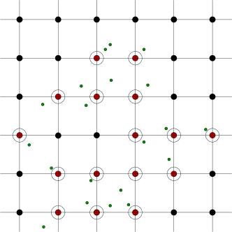
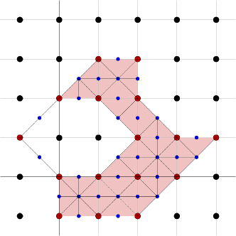
Figure 2: The left figure shows a two-dimensional grid, along with its cubical complex. The green points (small dots) denote the points in $P$ and the red vertices (encircled) are the active vertices. The figure on the right shows the generated simplicial complex. The blue vertices (small dots) are the barycenters of the active faces.

To complete the construction, we need to define simplicial maps $\mathcal{X}_{\alpha_{s}}\rightarrow\mathcal{X}_{\alpha_{s+1}}$. We show that such maps are induced by $g_{s}$.

Lemma 7.

Let $f$ be an active face of $\square_{s}$. Then, $g_{s}(f)$ is an active face of $\square_{s+1}$.

Proof.

From Lemma 3, $e:=g_{s}(f)$ is a face of $G_{s+1}$. If $e$ is a vertex, it is active, because $f$ contains at least one active vertex $v$, and $g_{s}(v)=e$ in this case. If $e$ is not a vertex, we assume for a contradiction that it is not active. Then, it contains a facet $e_{1}$ that contains all active vertices in $e$. Let $e_{2}$ denote the opposite facet. By Lemma 3, $f$ contains opposite facets $f_{1}$, $f_{2}$ such that $g_{s}(f_{1})=e_{1}$ and $g_{s}(f_{2})=e_{2}$. Since $f$ is active, both $f_{1}$ and $f_{2}$ contain active vertices, in particular, $f_{2}$ contains an active vertex $v$. But then, the active vertex $g_{s}(v)$ must lie in $e_{2}$, contracting the fact that $e_{1}$ contains all active vertices of $e$. ∎

Recall that a simplex $\sigma\in\mathcal{X}_{\alpha_{s}}$ is a flag $f_{0}\subseteq\ldots\subseteq f_{k}$ of active faces in $\square_{s}$. We set $\tilde{g}(\sigma)$ as the flag $g(f_{0})\subseteq\ldots\subseteq g(f_{k})$, which consists of active faces in $\square_{s+1}$ by Lemma 7, and hence is a simplex in $\mathcal{X}_{\alpha_{s+1}}$. It follows that $\tilde{g}:\mathcal{X}_{\alpha_{s}}\rightarrow\mathcal{X}_{\alpha_{s+1}}$ is a simplicial map. This finishes our construction of the simplicial tower $(\mathcal{X}_{\lambda 2^{s}})_{s\in\mathbb{Z}},$ with simplicial maps $\tilde{g}:\mathcal{X}_{\lambda 2^{s}}\rightarrow\mathcal{X}_{\lambda 2^{s+1}}$.

4.1 Interleaving

To relate our tower with the $L_{\infty}$-Rips filtration, we start by defining two acyclic carriers. We write $\alpha:=\alpha_{s}=\lambda 2^{s}$ to simplify notations.

• $C_{1}:\mathcal{R}^{\infty}_{\alpha}\rightarrow\mathcal{X}_{\alpha}$: let $\sigma=(p_{0},\ldots,p_{k})$ be any simplex of $\mathcal{R}^{\infty}_{\alpha}$. We set $C_{1}(\sigma)$ as the barycentric span of $U:=\{a_{s}(p_{0}),\ldots,a_{s}(p_{k})\}$, which is a subcomplex of $\mathcal{X}_{\alpha}$. $U$ lies in a face $f$ of $\square_{s}$ by Lemma 5 hence $C_{1}(\sigma)$ is also the $f$-local barycentric span of $U$. Using Lemma 4, $C_{1}(\sigma)$ is acyclic.

• $C_{2}:\mathcal{X}_{\alpha}\rightarrow\mathcal{R}^{\infty}_{2\alpha}$: let $\sigma$ be any flag $e_{0}\subseteq\ldots\subseteq e_{k}$ of $\mathcal{X}_{\alpha}$. Let $\{q_{0},\ldots,q_{m}\}$ be the set of active vertices of $e_{k}$. We set $C_{2}(\sigma):=\{b_{s}(q_{0}),\ldots,b_{s}(q_{m})\}$. With a simple triangle inequality, we see that $C_{2}(\sigma)$ is a simplex in $\mathcal{R}^{\infty}_{2\alpha}$, hence it is acyclic.

Using the Acyclic Carrier Theorem (Theorem 1), there exist chain maps $c_{1}:\mathcal{C}_{\ast}(\mathcal{R}^{\infty}_{\alpha})\rightarrow\mathcal{C}_{\ast}(\mathcal{X}_{\alpha})$ and $c_{2}:\mathcal{C}_{\ast}(\mathcal{X}_{\alpha})\rightarrow\mathcal{C}_{\ast}(\mathcal{R}^{\infty}_{2\alpha})$, which are carried by $C_{1}$ and $C_{2}$, respectively. Aggregating the chain maps, we have the following diagram:

(9)

where $inc$ corresponds to the inclusion chain map and $\tilde{g}$ denotes the chain map for the corresponding simplicial maps (we removed indices for readability). The chain complexes give rise to a diagram of the corresponding homology groups, connected by the induced linear maps $c_{1}^{\ast},c_{2}^{\ast},inc^{\ast},\tilde{g}^{\ast}$.

Lemma 8.

$inc^{\ast}=c_{2}^{\ast}\circ c_{1}^{\ast}$ and $\tilde{g}^{\ast}=c_{1}^{\ast}\circ c_{2}^{\ast}$. In particular, the persistence modules $\left(H(\mathcal{X}_{2^{s}})\right)_{s\in\mathbb{Z}}$ and $\left(H(\mathcal{R}^{\infty}_{\alpha})\right)_{\alpha\geq 0}$ are weakly $2$-interleaved.

Proof.

To prove the claim, we consider both triangles separately. We show that the chain maps $\tilde{g}$ and $c_{1}\circ c_{2}$ are carried by a common acyclic carrier. Then we show the same statement for $inc$ and $c_{2}\circ c_{1}$. The claim then follows from the Acyclic Carrier Theorem.

• Lower triangle: The map $C_{1}\circ C_{2}:\mathcal{X}_{\alpha}\rightarrow\mathcal{X}_{2\alpha}$ is an acyclic carrier, because $C_{2}(\sigma)$ is a simplex for any simplex $\sigma\in\mathcal{ULS}_{\alpha}$. Clearly, $C_{1}\circ C_{2}$ carries the map $c_{1}\circ c_{2}$. We show that it also carries $\tilde{g}$.

  Let $\sigma$ be a flag $f_{0}\subseteq\ldots\subseteq f_{k}$ in $\mathcal{X}_{\alpha}$ and let $V(f_{i})$ denote the active vertices of $f_{i}$. Then, $C_{1}\circ C_{2}(\sigma)$ is the barycentric span of

  $$U:=\{a_{s+1}\circ b_{s}(q)\mid q\in V(f_{k})\}=\{g_{s}(q)\mid q\in V(f_{k})\}$$

  (Lemma 6). On the other hand, $V(f_{i})\subseteq V(f_{k})$ and hence $g(V(f_{i}))\subseteq U$. Then, $g(f_{i})$ is spanned by $U$: indeed, since $f_{i}$ is active, $g(f_{i})$ is active and hence spanned by all active vertices, and it remains spanned if we remove all active vertices not in $U$, since they are not contained in $f_{i}$. It follows that the flag $g(f_{0})\subseteq\ldots\subseteq g(f_{k})$, which is equal to $\tilde{g}(\sigma)$, is in the barycentric span of $U$.

• Upper triangle: We define an acyclic carrier $D:\mathcal{R}^{\infty}_{2\alpha}\rightarrow\mathcal{R}^{\infty}_{4\alpha}$ which carries both $inc$ and $c_{2}\circ c_{1}$. Let $\sigma=(p_{0},\ldots,p_{k})\in\mathcal{R}^{\infty}_{2\alpha}$ be a simplex. The active vertices $U:=\{a(p_{0}),\ldots,a(p_{k})\}\subset G_{s+1}$ lie in a face $f$ of $G_{2\alpha}$, using Lemma 5. We can assume that $f$ is active, as otherwise, we pass to a facet of $f$ that contains $U$. We set $D(\sigma)$ as the simplex on the subset of points in $P$ whose closest grid point in $G_{s+1}$ lies in $U$. Using a simple application of triangle inequalities, $D(\sigma)\in\mathcal{R}^{\infty}_{4\alpha}$, so $D$ is an acyclic carrier. The $0$-simplices of $\sigma$ are a subset of $D(\sigma)$, so $D$ carries the map $inc$. We next show that $D$ carries $c_{2}\circ c_{1}$.

  Let $\delta$ be a simplex in $\mathcal{X}_{2\alpha}$ for which the chain $c_{1}(\sigma)$ takes a non-zero value. Since $c_{1}(\sigma)$ is carried by $C_{1}(\sigma)$, $\delta\in C_{1}(\sigma)$ which is the barycentric span of $V(f)$. Furthermore, for any $\tau\in C_{1}(\sigma)$, $C_{2}(\tau)$ is of the form $\{b(q_{0}),\ldots,b(q_{m})\}$ with $\{q_{0},\ldots,q_{m}\}\in V(f)$. It follows that $C_{2}(\tau)\subseteq D(\sigma)$. In particular, since $c_{2}$ is carried by $C_{2}$, $c_{2}(c_{1}(\sigma))\subseteq D(\sigma)$ as well.

∎

4.2 Scale balancing

We improve the approximation factor with a simple modification that we first explain in general. Let $(A_{\lambda\gamma^{k}})_{k\in\mathbb{Z}}$ and $(B_{\lambda\gamma^{k}})_{k\in\mathbb{Z}}$ be two simplicial towers with simplicial maps $f_{3}$ and $f_{4}$ respectively, with $\lambda,\gamma>0$. Assume that there exist interleaving linear maps $f_{1}^{\ast},f_{2}^{\ast}$ such that the diagram

(14)

commutes for all scales $\alpha=\lambda\gamma^{k}$, which implies that the persistence modules are weakly $\gamma$-interleaved. Defining another tower $(A^{\prime}_{\lambda\sqrt{\gamma}\gamma^{k}})_{k\in\mathbb{Z}}$ with $A^{\prime}_{\alpha}:=A_{\alpha/\sqrt{\gamma}}$, we obtain a diagram

(19)

which implies that the persistence modules are weakly $\sqrt{\gamma}$-interleaved. Therefore, scale balancing improves the interleaving ratio by only scaling the persistence module.

In our context, we can improve the weak $2$-interleaving of $(H(\mathcal{X}_{2^{k}\alpha}))_{k\in\mathbb{Z}}$ and $(H(\mathcal{R}^{\infty}_{\alpha}))_{\alpha\geq 0}$ to a weak $\sqrt{2}$-interleaving. Using the proximity results for persistence modules [6],

Theorem 9.

The persistence module $\big{(}H(\mathcal{X}_{2^{k}/\sqrt{2}})\big{)}_{k\in\mathbb{Z}}$ is a $3\sqrt{2}$- approximation of the $L_{\infty}$-Rips persistence module $\big{(}H(\mathcal{R}^{\infty}_{\alpha})\big{)}_{\alpha\geq 0}$.

For any pair of points $p,p^{\prime}\in\mathbb{R}^{d}$, it holds that $\|p-p^{\prime}\|_{2}\leq\|p-p^{\prime}\|_{\infty}\leq\sqrt{d}\,\|p-p^{\prime}\|_{2}$ which implies that the $L_{2}$- and the $L_{\infty}$-Rips complexes are strongly $\sqrt{d}$-interleaved. The scale balancing technique also works for strongly interleaved persistence modules and yields

Lemma 10.

$(H(\mathcal{R}_{\alpha/d^{0.25}}))_{\alpha\geq 0}$ is strongly $d^{0.25}$-interleaved with $(H(\mathcal{R}^{\infty}_{\alpha}))_{\alpha\geq 0}$.

Using Theorem 9, Lemma 10 and the fact that interleavings satisfy the triangle inequality [3, Theorem 3.3], we see that $(H(\mathcal{X}_{2^{k}/\sqrt{2}}))_{k\in\mathbb{Z}}$ is weakly $\sqrt{2}d^{0.25}$-interleaved with the scaled Rips module $(H(\mathcal{R}_{\alpha/d^{0.25}}))_{\alpha\geq 0}$. We can remove the scaling in the Rips filtration simply by multiplying both sides with $d^{0.25}$ and obtain our final approximation result.

Theorem 11.

The persistence module $\big{(}H(\mathcal{X}_{\frac{2^{k}\sqrt[4]{d}}{\sqrt{2}}})\big{)}_{k\in\mathbb{Z}}$ is a $3\sqrt{2}d^{0.25}$-approximation of the Euclidean Rips persistence module $\big{(}H_{\ast}(\mathcal{R}_{\alpha})\big{)}_{\alpha\geq 0}$.

5 Size and computation

Set $n:=|P|$ and let $CP(P)$ denote the closest pair distance of $P$. At scale $\alpha_{0}:=\frac{CP(P)}{3d}$ and lower, no $d$-cube of the cubical complex contains more than one active vertex, so the approximation complex consists of $n$ isolated $0$-simplices. At scale $\alpha_{m}:=diam(P)$ and higher, points of $P$ map to active vertices of a common face by Lemma 5, so the generated complex is acyclic using Lemma 4. We inspect the range of scales $[\alpha_{0},\alpha_{m}]$ to construct the tower, since the barcode is explicitly known for scales outside this range. The total number of scales is $\lceil\log_{2}\alpha_{m}/\alpha_{0}\rceil=\lceil\log_{2}\Delta+\log_{2}3d\rceil=O(\log\Delta+\log d)$.

5.1 Size of the tower

Recall that the size of a tower is the number of simplices that do not have a preimage. We start by considering the case of $0$-simplices.

Lemma 12.

The number of $0$-simplices included in the tower is at most $n2^{O(d)}$.

Proof.

Recall that the $0$-simplices of $\mathcal{X}_{\alpha}$ are the active faces of the cubical complex $\square$ at the same scale, and that the simplicial map $\tilde{g}$ restricted to the $0$-simplices corresponds to the cubical map $g$.

We first consider the active vertices: at scale $\alpha_{0}$, there are $n$ inclusions of $0$-simplices in the tower, due to $n$ active vertices. By Lemma 2, $g$ is surjective on the active vertices of $\square$ (for any scale). Hence, no further active vertices are added to the tower.

It remains to count the active faces of dimension $\geq 1$ without preimage. We will use a charging argument, charging the existence of such an active face to one of the points in $P$, charging each point at most $3^{d}$ times. For that, we fix an arbitrary total order $\prec$ on $P$. Each active vertex on any scale has a non-empty subset of $P$ in its Voronoi region; we call the maximal such point with respect to $\prec$ the representative. For an active face $f$ without preimage under $g$, $f$ has at least two incident active vertices, with distinct representatives. We charge the inclusion of $f$ to the minimal representative among the incident active vertices.

Let $M$ be the number of incident faces of a vertex in the cubical grid $\square$ (for any scale). As one can easily see with combinatorial arguments, $M=3^{d}=2^{O(d)}$. Assume for a contradiction that a a point $p\in P$ is charged more than $M$ times. Whenever any face $f_{i}$ is charged to $p$, there is an active vertex $v_{i}$ whose representative is $p$. We enumerate these as the set of active vertices $\{v_{0},\ldots,v_{m}\}$ on the scales $\alpha_{0},\ldots,\alpha_{m}$ such that $p$ is the representative of $v_{i}$ on scale $\alpha_{i}$. Naturally, for any $v_{i}$ and $v_{j}$, there is a canonical isomorphism between the $M$ faces incident to $v_{i}$ and the $M$ faces incident to $v_{j}$.

Since we assumed that $p$ is charged for $>M$ active faces, by pigeonhole principle, there must be two vertices $v_{i}$ and $v_{j}$ with $i<j$ such that a pair of isomorphic incident faces are charged for $v_{i}$ and for $v_{j}$. There is a sequence of isomorphic faces $f_{i},f_{i+1},\ldots,f_{j}$ corresponding to $v_{i},v_{i+1}\ldots,v_{j}$, respectively, such that $p$ is charged for $f_{i}$ and $f_{j}$. Since $f_{i}$ and $f_{j}$ have both no preimage, there must be some $f_{\ell}$ with $i<\ell<j$ such that $f_{\ell}$ is not active. That means, however, that the Voronoi region of $v_{\ell}$ is the union of at least two Voronoi regions of vertices incident to $v_{i}$. In that case, because we choose the representative by minimizing over the maximal representatives, so $p$ is not the representative of $v_{\ell}$, and hence, not of $v_{j}$. This is a contradiction to our claim, so $M$ can not be charged more than $M$ times. ∎

The next lemma follows from a simple combinatorial counting argument for the number of flags in a $d$-dimensional cube.

Lemma 13.

Each $0$-simplex of $\mathcal{X}_{\alpha}$ has at most $2^{O(d\log k)}$ incident $k$-simplices.

Proof.

A $0$-simplex in $\mathcal{X}\alpha$ corresponds to an active face $f$ in a cubical complex $\square$. An incident simplex corresponds to an active flag of $\square$ involving $f$. Let $c$ be a $d$-cube of $\square$ that contains $f$. We simply count the number of flags of length $(k+1)$ contained in $c$ (regardless of whether they contain $f$ or not) and show that the number is $2^{O(d\log k)}$. Since $f$ is contained in at most $2^{d}$ $d$-cubes, the bound follows.

To count the number of flags containing $c$, we us similar ideas as in [10]: first fix a vertex $v$ of $c$ and count the flags of the form $v\subseteq\ldots\subseteq c$. Every $\ell$-face in $c$ incident to $v$ corresponds to a subset of $\ell$ coordinate indices, in the sense that the coordinates not chosen are fixed to the coordinates of $v$ for the face. With this correspondence, it is not hard to see that a flag from $v$ to $c$ of length $k+1$ corresponds to an ordered $k$-partition of $\{1,\ldots,d\}$. The number of such partitions is known as $k!$ times the quantity $\left\{\begin{array}[]{c}d\\ k\end{array}\right\}$, which is the Stirling number of second kind, and is upper bounded by $2^{O(d\log k)}$ [7]. Since $c$ has $2^{d}$ vertices, the total number of flags of the form $v\subseteq\ldots\subseteq c$ with any vertex $v$ is hence $2^{d}k!2^{O(d\log k)}=2^{O(d\log k)}$.

For flags which do not start with a vertex and do not end with $c$, we can simply extend by adding a vertex and/or the $d$-cube and obtain flags of length $k+2$ or $k+3$. The same argument as above shows again that the number of such flags is bounded by $2^{O(d\log k)}$ which proves the claim. ∎

Theorem 14.

The $k$-skeleton of the tower has size at most $n2^{O(d\log k)}$.

Proof.

Let $\sigma=f_{0}\subseteq\ldots\subseteq f_{k}$ be a flag included at some scale $\alpha$. The crucial insight is that this can only happen if at least one face $f_{i}$ in the flag is included in the tower at the same scale. Indeed, if each $f_{i}$ has a preimage $e_{i}$ on the previous scale, then $e_{0}\subseteq\ldots\subseteq e_{k}$ is a flag on the previous scale which maps to $\sigma$ under $\tilde{g}$.

We charge the inclusion of the flag to the inclusion of $f_{i}$. By Lemma 13, the $0$-simplex $f_{i}$ of $\mathcal{X}$ is charged at most $\sum_{i=1}^{k}2^{O(d\log i)}=2^{O(d\log k)}$ times in this way, and by Lemma 12, there are at most $n2^{O(d)}$ $0$-simplices that can be charged. ∎

5.2 Computing the tower

Recall from the construction of the grids that $G_{s+1}$ is built from $G_{s}$ using an arbitrary translation vector $(\pm 1,\ldots,\pm 1)\in\mathbb{Z}^{d}$. In our algorithm, we pick the components of this translation vector uniformly at random, and independently for each scale.

Recall the cubical map $g_{s}:\square_{s}\rightarrow\square_{s+1}$ from Section 3. For a fixed $s$, we denote by $g^{(j)}:\square_{s}\rightarrow\square_{s+j}$ the $j$-fold composition of $g$, that is $g^{(j)}=g_{s+j-1}\circ g_{s+j-2}\circ\ldots\circ g_{s}$.

Lemma 15.

For a $k$-face $f$ of $\square_{s}$, let $Y$ be the minimal integer $j$ such that $g^{(j)}(f)$ is a vertex. Then $E[Y]\leq 3\log k$.

Proof.

Without loss of generality, assume that the grid under consideration is $\mathbb{Z}^{d}$ and $f$ is the $k$-face spanned by the vertices $\{\underbrace{\pm 1,\ldots,\pm 1}_{k},0,\ldots,0\}$. The proof for the general case is analogous.

Let $y_{1}\in\{-1,1\}$ denote the randomly chosen shift of the first coordinate. If $y_{1}=1$, the grid $G^{\prime}$ on the next scale has a grid point with $x_{1}$-coordinate $1/2$. Clearly, the closest grid point in $G^{\prime}$ to the origin is of the form $(+1/2,\pm 1/2,\ldots,\pm 1/2)$, and thus, this point is also closest to $(1,0,0,\ldots,0)$. The same is true for any point $(0,\ast,\ldots,\ast)$ and its corresponding point $(1,\ast,\ldots,\ast)$ on the opposite facet. Hence, for $y_{1}=1$, $g(f)$ is a face where all points have the same $x_{1}$-coordinate.

Contrarily, if $y_{1}=-1$, the origin is mapped to some point $(-1/2,\pm 1/2,\ldots,\pm 1/2)$ and $(1,0,\ldots,0)$ is mapped to $(3/2,\pm 1/2,\ldots,\pm 1/2)$, as one can directly verify. Hence, in this case, in $g(f)$, points do not all have the same $x_{1}$ coordinate.

We say that the $x_{1}$-coordinate collapses in the first case and does not collapse in the second. Because the shift is chosen uniformly at random for each scale, the probability that $x_{1}$ did not collapse after $j$ iterations is $1/2^{j}$.

$f$ spans $k$ coordinate directions, so it must collapse along each such direction to contract to a vertex. Once a coordinate collapses, it stays collapsed at all higher scales. As the shift is independent for each coordinate direction, the probability of a collapse is the same along all coordinate directions that $f$ spans. Using union bound, the probability that $g^{j}(f)$ has not collapsed to a vertex is at most $k/2^{j}$. With $Y$ as in the statement of the lemma $P(Y\geq j)\leq k/2^{j}$. Hence,

$$E[Y]=\sum_{j=1}^{\infty}jP(Y=j) =\sum_{j=1}^{\infty}P(Y\geq j)\leq\log k+\sum_{c=1}^{\infty}\sum_{j=c\log k}^{(c+1)\log k}P(Y\geq j)$$

$$\leq\log k+\sum_{c=1}^{\infty}\sum_{j=c\log k}^{(c+1)\log k}P(Y\geq c\log k)\leq\log k+\sum_{c=1}^{\infty}\log k\frac{k}{2^{c\log k}}$$

$$\leq\log k+\log k\sum_{c=0}^{\infty}\frac{1}{k^{c}}\leq\log k+2\log k\leq 3\log k.$$

∎

As a consequence of the lemma, the expected “lifetime” of $k$-simplices in our tower with $k>0$ is rather short: Given a flag $e_{0}\subseteq\ldots\subseteq e_{\ell}$, the face $e_{\ell}$ will be mapped to a vertex after $O(\log d)$ steps, and so will be all its sub-faces, turning the flag into a vertex. It follows that summing up the total number of $k$-simplices with $k>0$ over all $\mathcal{X}_{\alpha}$ yields an upper bound of $n2^{O(d\log k)}$ as well.

Algorithm description

We first specify what it means to “compute” the tower. We make use of the fact that a simplicial map between simplicial complexes can be written as a composition of simplex inclusions and contractions of $0$-simplices [8, 12]. That is, when passing from a scale $\alpha_{s}$ to $\alpha_{s+1}$, it suffices to specify which pairs of $0$-simplices in $\mathcal{X}_{\alpha_{s}}$ are mapped to the same image under $\tilde{g}$ and which simplices in $\mathcal{X}_{\alpha_{s+1}}$ are included.

The input is a set of $n$ points $P\subset\mathbb{R}^{d}$. The output is a list of events, where each event is of one of the three following types: a scale event defines a real value $\alpha$ and signals that all upcoming events happen at scale $\alpha$ (until the next scale event). An inclusion event introduces a new simplex, specified by the list of $0$-simplices on its boundary (we assume that every $0$-simplex is identified by an integer). A contraction event is a pair of $0$-simplices $(i,j)$ and signifies that $i$ and $j$ are identified as the same from that scale.

In a first step, we calculate the range of scales that we are interested in. We compute a $2$-approximation of $diam(P)$ by taking any point $p\in P$ and calculating $max_{q\in P}\|p-q\|$. Then we compute $CP(P)$ using a randomized algorithm in $n2^{O(d)}$ expected time [14].

Next, we proceed scale-by-scale and construct the list of events accordingly. On the lowest scale, we simply compute the active vertices by point location for $P$ in a cubical grid, and enlist $n$ inclusion events (this is the only step where the input points are considered in the algorithm). We use an auxiliary container $S$ and maintain the invariant that whenever a new scale is considered, $S$ consists of all simplices of the previous scale, sorted by dimension. In $S$, for each $0$-simplex, we store an id and a coordinate representation of the active face to which it corresponds. Every $\ell$-simplex with $\ell>0$ is stored just as a list of integers, denoting its boundary $0$-simplices. We initialize $S$ with the $n$ $0$-simplices at the lowest scale.

Let $\alpha<\alpha^{\prime}$ be any two consecutive scales with $\square,\square^{\prime}$ the respective cubical complexes and $\mathcal{X},\mathcal{X}^{\prime}$ the approximation complexes, with $\tilde{g}:\mathcal{X}\rightarrow\mathcal{X}^{\prime}$ being the simplicial map connecting them. Suppose we have already constructed all events at scale $\alpha$. We enlist the scale event for $\alpha^{\prime}$. Then, we enlist the contraction events. For that, we iterate through the $0$-simplices of $\mathcal{X}$ and compute their value under $g$, using point location in a cubical grid. We store the results in a list $S^{\prime}$ (which contains the simplices of $\mathcal{X}^{\prime}$). If for a $0$-simplex $j$, $g(j)$ is found to be equal to $g(i)$ for a previously considered $0$-simplex, we choose the minimal such $i$ and enlist a contraction event for $i$ and $j$.

We turn to the inclusion events and start with the case of $0$-simplices. Every $0$-simplex is an active face at scale $\alpha^{\prime}$ and must contain an active vertex, which is also a $0$-simplex of $\mathcal{X}^{\prime}$. We iterate through the elements in $S^{\prime}$. For each active vertex $v$ encountered, we go over all faces of the cubical complex $\square^{\prime}$ that contain $v$ as vertex and check whether they are active. For every active face encountered that is not in $S^{\prime}$ yet, we add it to $S^{\prime}$ and enlist an inclusion event of a new $0$-simplex. At termination, all $0$-simplices of $\mathcal{X}^{\prime}$ have been detected.

Next, we iterate over the simplices of $S$ of dimension $\geq 1$ and compute their image under $\tilde{g}$, and store the result in $S^{\prime}$. To find the simplices of dimension $\geq 1$ included at $\mathcal{X}^{\prime}$, we exploit our previous insight that they contain at least one $0$-simplex that is included at the same scale (see the proof of Theorem 14). Hence, we iterate over the $0$-simplices included in $\mathcal{X}^{\prime}$ and proceed inductively in dimension. Let $v$ be the current $0$-simplex under consideration; assume that we have found all $(p-1)$-simplices in $\mathcal{X}^{\prime}$ that contain $v$. Each such $(p-1)$-simplex $\sigma$ is a flag in $\square^{\prime}$. We iterate over all faces $e$ that extend $\sigma$ to a flag of length $p+1$. If $e$ is active, we found a $p$-simplex in $\mathcal{X}^{\prime}$. If this simplex is not in $S^{\prime}$ yet, we add it and enlist an inclusion event for it. We also enqueue the simplex in our inductive procedure, to look for $(p+1)$-simplices in the next iteration. At the end of the procedure, we have detected all simplices in $\mathcal{X}^{\prime}$ without preimage, and $S^{\prime}$ contains all simplices of $\mathcal{X}^{\prime}$. We set $S\leftarrow S^{\prime}$ and proceed to the next scale. This ends the description of the algorithm.

Theorem 16.

To compute the $k$-skeleton, the algorithm takes time $\big{(}n2^{O(d)}\log\Delta+2^{O(d)}M\big{)}$ time in expectation and $M$ space, where $M$ is the size of the tower. In particular, the expected time is bounded by $\big{(}n2^{O(d)}\log\Delta+n2^{O(d\log k)}\big{)}$ and the space is bounded by $n2^{O(d\log k)}$.

Proof.

In the analysis, we ignore the costs of point locations in grids, checking whether a face for being active, and searches in data structures $S$, since all these steps have negligible costs when appropriate data structures are chosen.

Computing the image of a $0$-simplex of $\mathcal{X}$ costs $O(2^{d})$ time. Moreover, there are at most $n2^{O(d)}$ vertices altogether in the tower, so this bound in particular holds on each scale. Hence, the contraction events on a fixed scales can be computed in $n2^{O(d)}$. Finding new $0$-simplices requires iterating over the cofaces of a vertex in a cubical complex. There are $3^{d}$ such cofaces. This has to be done for a subset of the $0$-simplices in $\mathcal{X}^{\prime}$, so the running time is also $n2^{O(d)}$. Since there are $O(\log\Delta+\log d)$ scales considered, these steps require $n2^{O(d)}\log\Delta$ over all scales.

Computing the image of $\tilde{g}$ for a fixed scale costs at most $O(2^{d}|\mathcal{X}|)$. $M$ is the size of the tower, that is, the simplices without preimage, and $I$ the set of scales considered, so the expected bound for $\sum_{\alpha\in I}|\mathcal{X}_{\alpha}|=O(\log dM)$, because every simplex has an expected lifetime of at most $3\log d$ by Lemma 15. Hence, the cost of these steps is bounded by $2^{O(d)}M$.

In the last step of the algorithm, we consider a subset of simplices of $\mathcal{X}^{\prime}$. For each one, we iterate over a collection of faces in the cubical complex of size at most $2^{O}(d)$. Hence, this step is also bounded by $O(2^{O(d)}|\mathcal{X}|)$ per scale, and hence bounded $2^{O(d)}M$ as well.

For the space complexity, the auxiliary data structure $S$ gets as large as $\mathcal{X}$, which is clearly bounded by $M$. For the output complexity, the number of contraction events is smaller than the number of inclusion events, because every contraction removes a $0$-simplex that has been included before. The number of inclusion events is the size of the tower. The number of scale events as described is $O(\log\Delta+\log d)$. However, it is simple to get rid of this factor by only including scale events in the case that at least one inclusion/contraction takes place at this scale. The space complexity bound follows. ∎

6 Conclusion

We gave an approximation scheme for the Rips filtration, with improved approximation ratio, size and computational complexity than previous approaches for the case of high-dimensional point clouds. Moreover, we introduced the technique of using acyclic carriers to prove interleaving results. We point out that, while the proof of the interleaving in Section 4.1 is still technically challenging, it greatly simplifies by the usage of acyclic carriers; defining the interleaving chain maps explicitly significantly blows up the analysis. There is also no benefit in knowing the interleaving maps because they are only required for the analysis, not for the computation.

Our tower is connected by simplicial maps; there are (implemented) algorithms to compute the barcode of such towers [8, 12]. It is also quite easy to adapt our tower construction to a streaming setting [12], where the output list of events is passed to an output stream instead of being stored in memory.

An interesting question is whether persistence can be computed efficiently for more general chain maps, which would allow more freedom in building approximation schemes.

Acknowledgments

Michael Kerber is supported by the Austrian Science Fund (FWF) grant number P 29984-N35. Sharath Raghvendra acknowledges support of NSF CRII grant CCF-1464276.

References

- [1] M. Botnan and G. Spreemann. Approximating Persistent Homology in Euclidean space through collapses. Applied Algebra in Engineering, Communication and Computing, 26(1-2):73–101, 2015.
- [2] P. Bubenik, V. de Silva, and J. Scott. Metrics for Generalized Persistence Modules. Foundations of Computational Mathematics, 15(6):1501–1531, 2015.
- [3] P. Bubenik and J.A. Scott. Categorification of Persistent Homology. Discrete & Computational Geometry, 51(3):600–627, 2014.
- [4] G. Carlsson. Topology and Data. Bulletin of the American Mathematical Society, 46:255–308, 2009.
- [5] N.J. Cavanna, M. Jahanseir, and D. Sheehy. A Geometric Perspective on Sparse Filtrations. In Proceedings of the 27th Canadian Conference on Computational Geometry (CCCG 2015).
- [6] F. Chazal, D. Cohen-Steiner, M. Glisse, L.J. Guibas, and S.Y. Oudot. Proximity of Persistence Modules and their Diagrams. In Proceedings of the ACM Symposium on Computational Geometry (SoCG 2009), pages 237–246, 2009.
- [7] A. Choudhary, M. Kerber, and S. Raghvendra. Polynomial-sized topological approximations using the Permutahedron. In Proceedings of the 32nd International Symposium on Computational Geometry (SoCG 2016), pages 31:1–31:16, 2016.
- [8] T.K. Dey, F. Fan, and Y. Wang. Computing Topological Persistence for Simplicial maps. In Proceedings of the ACM Symposium on Computational Geometry (SoCG 2014), pages 345–354, 2014.
- [9] H. Edelsbrunner and J. Harer. Computational Topology - An Introduction. American Mathematical Society, 2010.
- [10] H. Edelsbrunner and M. Kerber. Dual Complexes of Cubical Subdivisions of . Discrete & Computational Geometry, 47(2):393–414, 2012.
- [11] H. Edelsbrunner, D. Letscher, and A. Zomorodian. Topological Persistence and Simplification. Discrete & Computational Geometry, 28(4):511–533, 2002.
- [12] M. Kerber and H. Schreiber. Barcodes of Towers and a Streaming Algorithm for Persistent Homology. In Proceedings of the 33rd International Symposium on Computational Geometry (SoCG), pages 57:1–57:15, 2017.
- [13] M. Kerber and R. Sharathkumar. Approximate Čech Complex in Low and High Dimensions. In International Symposium on Algorithms and Computation (ISAAC), pages 666–676, 2013.
- [14] S. Khuller and Y. Matias. A Simple Randomized Sieve Algorithm for the Closest-Pair Problem. Information and Computation, 118(1):34 – 37, 1995.
- [15] J.R. Munkres. Elements of algebraic topology. Westview Press, 1984.
- [16] D. Sheehy. Linear-size Approximations to the Vietoris-Rips Filtration. Discrete & Computational Geometry, 49(4):778–796, 2013.