Regge phenomenology in $\pi^{0}$ and $\eta$ photoproduction

Abstract

The $\gamma N\to\pi^{0}N$ and $\gamma N\to\eta N$ reactions at photon beam energies above 4 GeV are investigated within Regge models. The models include $t$-channel exchanges of vector ($\rho$ and $\omega$) and axial vector ($b_{1}$ and $h_{1}$) mesons. Moreover, Regge cuts of $\rho{\mathbb{P}}$, $\rho f_{2}$, $\omega{\mathbb{P}}$, and $\omega f_{2}$ are investigated. A good description of differential cross sections and polarization observables at photon beam energies from 4 to 15 GeV can be achieved.

I Introduction

Meson photo- and electroproduction processes are closely related to the long-range structure and dynamics of hadrons. The phenomenology of these reactions changes at center of mass energies of about $W\approx 3$ GeV, roughly separating resonance and continuum regions.

Below $W\approx 3$ GeV, which corresponds to photon beam energies below $E_{\gamma}\approx 4$ GeV, the reaction dynamics is characterized by the excitation of individual s-channel baryon resonances with definite quantum numbers on top of smooth, non-resonant background. Within the last two decades, new data on photoinduced meson production has become the major source of information for baryon spectroscopy. At the electron accelerator labs ELSA, JLab and MAMI extensive developments in beam and target polarization techniques have been undertaken and an enormous amount of data with different types of polarization has been obtained, especially for $\pi$, $\eta$ and $K$ photoproduction Crede:2013sze . Above this resonance region, at $W\gtrsim 3$ GeV, the reaction dynamics changes and can be described most effectively by particle (reggeon) exchanges in the crossed $t$-channel Irving:1977ea . Experimental data on $\pi$ and $\eta$ photoproduction in this high-energy region were mainly measured in the 1970s at DESY DESY:1970 ; DESY:1973 ; DESY:1968 and SLAC SLAC:1971 , but only a limited amount of target and recoil polarization data is available. Only recently, the new GlueX experiment in Hall-D at JLab started data taking and first results on differential cross sections with a linearly polarized photon beam at $E_{\gamma}$= 8.7 GeV were already obtained GlueX:2017 .

The resonance and the continuum regions are of course not independent from each other but analytically connected via dispersion relations Aznauryan:2002gd ; Aznauryan:2003zg ; Pasquini:2006yi ; Pasquini:2007fw or finite energy sum rules Dolen:1967jr ; Mathieu:2015-2 ; Nys:2017 . The motivation for this study is therefore twofold. Firstly, with view to new results on unpolarized cross sections and photon beam asymmetries expected from GlueX in the next years, we want to obtain a deeper understanding of the high-energy Regge phenomenology.

Secondly, we consider a good description of the high-energy data as an important prerequisite for a high-quality baryon resonance analysis at lower energies. In particular in $\eta$, $\eta^{\prime}$ and $K$ photoproduction a good knowledge about Regge contributions to non-resonant background amplitudes is crucial for a reliable extraction of resonance parameters.

The main features of our models are Regge trajectories from $\omega$ and $\rho$ vector mesons and Regge cuts arising from the exchange of two Reggeons. We compare different approaches to available high-energy data for $\pi^{0}$ and $\eta$ photoproduction at lab energies above 4 GeV. We show that in particular polarization observables, as photon beam and target asymmetries or recoil polarization, are crucial to distinguish between the different models.

This paper is organized as follows. In section II we briefly introduce kinematics, polarization observables and photoproduction amplitudes. In section III we compare different Regge approaches with Regge poles and Regge cuts and discuss the various trajectories. In section IV we compare different models to high-energy data of $\pi^{0}$ and $\eta$ photoproduction for unpolarized cross sections and polarization observables.

II Kinematics, observables and amplitudes

II.1 Kinematics

Let us first define the kinematics of $\pi$ and $\eta$ photoproduction reactions on a nucleon,

$$\gamma(k)+N(p_{i})\to\pi/\eta(q)+N^{\prime}(p_{f})\ ,$$ (1)

where the variables in brackets denote the four-momenta of the participating particles. The familiar Mandelstam variables are

$$s=(p_{i}+k)^{2},\quad t=(q-k)^{2},\quad u=(p_{i}-q)^{2}\,,$$ (2)

where the sum of the Mandelstam variables is given by the sum of the external masses. The crossing symmetrical variable $\nu$ is related to the photon lab energy $E_{\gamma}^{lab}$ by

$$\nu=\frac{(s-u)}{4M_{N}}=E_{\gamma}^{lab}+\frac{t-\mu^{2}}{4M_{N}}\,,$$ (3)

where $M_{N}$ and $\mu$ are nucleon and meson masses ($\pi$ or $\eta$), respectively.

II.2 Observables

In photoproduction of pseudoscalar mesons a total of 16 polarization observables can be measured, which include the unpolarized cross section, three single-polarization and 12 double-polarization observables. By considering only beam and target polarization, the cross section depends on 8 observables, which can be separated by circular, $P_{\odot}$, and linear, $P_{T}$, photon beam polarization and the three components $P_{x},P_{y},P_{z}$ of the target polarization vector:

$$\frac{d\sigma}{d\Omega} = \sigma_{0}\left\{1-P_{T}\Sigma\cos 2\varphi\right.$$ (4)

$$+P_{x}\left(-P_{T}H\sin 2\varphi+P_{\odot}F\right)$$

$$-P_{y}\left(-T+P_{T}P\cos 2\varphi\right)$$

$$\left.-P_{z}\left(-P_{T}G\sin 2\varphi+P_{\odot}E\right)\right\}\,.$$

The $z$-axis is pointing into the direction of the incoming photon. The $\hat{y}$ direction is perpendicular to the reaction plane, $\hat{y}=\hat{z}\times\hat{q}$, defined by the incoming photon and the direction of the outgoing meson $\hat{q}$. The $x$-axis is given by

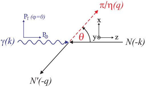
Figure 1: Kinematics for $\pi^{0}$ or $\eta$ photoproduction and frames for beam and target polarization.

$\hat{x}=\hat{y}\times\hat{z}$. The orientation of the linear polarization vector of the photon beam relative to the production plane is given by the angle $\varphi$, see Fig. 1. Expressions of the polarization observables in terms of amplitudes are given in the appendix.

II.3 Invariant amplitudes and fixed-$t$ dispersion relations

The electromagnetic current for pseudoscalar meson photoproduction can be expressed in terms of four invariant amplitudes $A_{i}(\nu,t)$ CGLN:1957 ,

$$J^{\mu}=\sum_{i=1}^{4}A_{i}(\nu,t)\,M^{\mu}_{i},$$ (5)

with the gauge-invariant four-vectors $M^{\mu}_{i}$ given by

$$M^{\mu}_{1} = -\frac{1}{2}i\gamma_{5}\left(\gamma^{\mu}\sl{k}-\sl{k}\gamma^{\mu}\right)\,,$$

$$M^{\mu}_{2} = 2i\gamma_{5}\left(P^{\mu}\,k\cdot(q-\frac{1}{2}k)-(q-\frac{1}{2}k)^{\mu}\,k\cdot P\right)\,,$$

$$M^{\mu}_{3} = -i\gamma_{5}\left(\gamma^{\mu}\,k\cdot q-\sl{k}q^{\mu}\right)\,,$$

$$\ M^{\mu}_{4} = -2i\gamma_{5}\left(\gamma^{\mu}\,k\cdot P-\sl{k}P^{\mu}\right)-2M_{N}\,M^{\mu}_{1}\,,$$ (6)

where $P^{\mu}=(p_{i}^{\mu}+p_{f}^{\mu})/2$.

The invariant amplitudes $A_{i}(\nu,t)$ have definite crossing symmetry and satisfy the following dispersion relations at fixed $t$:

$${\rm Re}A_{i}(\nu,t)=A_{i}^{pole}(\nu,t)+\frac{2}{\pi}\;{\cal P}\int_{\nu_{thr}}^{\infty}{\rm d}\nu^{\prime}\;\frac{\nu^{\prime}\,{\rm Im}A_{i}(\nu^{\prime},t)}{\nu^{\prime 2}-\nu^{2}}\,,$$ (7)

for the crossing-even amplitudes, $A_{1,2,4}$, and

$${\rm Re}A_{3}(\nu,t)=A_{3}^{pole}(\nu,t)+\frac{2\nu}{\pi}\;{\cal P}\int_{\nu_{thr}}^{\infty}{\rm d}\nu^{\prime}\;\frac{{\rm Im}A_{3}(\nu^{\prime},t)}{\nu^{\prime 2}-\nu^{2}}\,$$ (8)

for the crossing-odd amplitude $A_{3}$ Pasquini:2006yi .

III $t$-channel exchanges

III.1 Vector and axial-vector poles in the $t$ channel

The amplitudes of pseudoscalar meson photoproduction typically contain contributions from nucleon resonance excitations and a non-resonant background from Born terms and $t$-channel meson exchanges. In the current approach we want to consider only amplitudes at high energies beyond the nucleon resonance region. Furthermore, we neglect Born terms, which are practically zero for $\eta$ photoproduction MAID:2003 . Also in $\pi^{0}$ photoproduction they only play a minor role at forward angles.

We concentrate on $t$-channel contributions and will firstly consider the exchange of vector and axial vector mesons in terms of single pole Feynman diagrams, see Fig. 2(a) as an example for $\rho$ and $\omega$ meson exchange.

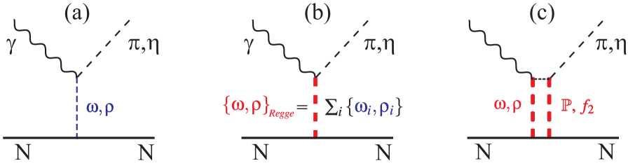
Figure 2: $t$-channel contributions to $\eta$ photoproduction from single poles (a), Regge poles (b), and Regge cuts (c). An example for $\rho$ and $\omega$ meson exchange and $\mathbb{P}$ and $f_{2}$ mesons for rescattering of two Reggeons.

Expressed in terms of invariant amplitudes $A_{i}$, these $t$-channel Feynman diagrams obtain the simple form

$$A_{1}(t) = \frac{e\,\lambda_{V}\,g_{V}^{\mathfrak{t}}}{2\mu M_{N}}\;\frac{t}{t-M_{V}^{2}}\,,$$ (9)

$$A_{2}^{\prime}(t) = -\frac{e\,\lambda_{A}\,g_{A}^{\mathfrak{t}}}{2\mu M_{N}}\;\frac{t}{t-M_{A}^{2}}\,,$$ (10)

$$A_{3}(t) = \frac{e\,\lambda_{A}\,g_{A}^{v}}{\mu}\;\frac{1}{t-M_{A}^{2}}\,,$$ (11)

$$A_{4}(t) = \frac{-e\,\lambda_{V}\,g_{V}^{v}}{\mu}\;\frac{1}{t-M_{V}^{2}}\,,$$ (12)

where $\lambda_{V(A)}$ denotes the electromagnetic coupling of the vector ($V$) or axial ($A$) vector mesons with masses $M_{V(A)}$. The constants $g_{V(A)}^{v(\mathfrak{t})}$ denote their vector $(v)$ or tensor $(\mathfrak{t})$ couplings to the nucleon. In order to separate the vector and tensor contributions from individual mesons, we followed Ref. Nys:2017 and introduced the amplitude

$$A_{2}^{\prime}(t)=A_{1}(t)+t\,A_{2}(t)\,,$$ (13)

which has only contributions from the tensor coupling of an axial vector exchange.

Table 1: Isospin $I$, $G$-parity, spin $J$, parity $P$, and charge conjugation $C$ quantum numbers for pseudoscalar, vector and axial vector mesons.

	$\gamma$	$\pi^{0}$	$\eta$	$\rho(770)$	$\omega(782)$	$\phi(1020)$	$b_{1}(1235)$	$h_{1}(1170)$	$a_{1}(1260)$	$f_{1}(1285)$
$I^{G}$	$0,1$	$1^{-}$	$0^{+}$	$1^{+}$	$0^{-}$	$0^{-}$	$1^{+}$	$0^{-}$	$1^{-}$	$0^{+}$
$J^{PC}$	$1^{--}$	$0^{-+}$	$0^{-+}$	$1^{--}$	$1^{--}$	$1^{--}$	$1^{+-}$	$1^{+-}$	$1^{++}$	$1^{++}$

There are three vector mesons $\rho$, $\omega$, $\phi$ and four axial vector mesons $b_{1}$, $h_{1}$, $a_{1}$, $f_{1}$, that could be used in our approach. The details on the quantum numbers are listed in Table 1. For the nucleon vertex, the axial-vector coupling $\gamma^{\mu}\gamma_{5}$ is $C$-even and the pseudo-tensor coupling $\sigma^{\mu\nu}\gamma_{5}$ is $C$-odd Kaskulov:2010 . Therefore, due to charge conjugation conservation, the $C$-odd $b_{1}$ and $h_{1}$ mesons couple to the nucleon via the tensor coupling only and can contribute to the $A_{2}$ ($A_{2}^{\prime}$) amplitude (see equations (10) and (13)), whereas $C$-even $a_{1}$ and $f_{1}$ mesons via the vector coupling only and, in principal, can contribute to the $A_{3}$ amplitude. However, the quantum numbers $I^{G}$ should be equal to $0^{-}$ or $1^{+}$ for $\pi^{0}$ and $\eta$ photoproduction on the nucleon. Consequently, $a_{1}(I^{G}=1^{-})$ and $f_{1}(I^{G}=0^{+})$ are excluded in our case. The $a_{1}$ is a good candidate for charged-pion photoproduction and $f_{1}$ for the $\gamma p\to\rho^{0}p$ channel Pasquini:2006yi . Therefore, there is no candidate left among vector and axial vector mesons which could contribute to $A_{3}$.

The $\phi$ meson could in principle contribute to $A_{1}$ and $A_{4}$. However, being practically a pure strange quark-antiquark state, a very small coupling to the nucleon is expected and it is commonly neglected in $\pi^{0}$ and $\eta$ photoproduction.

The invariant amplitudes (9)-(12) contain only the product of electromagnetic and hadronic coupling constants. We have fixed one of them and determined the second one by the fit. In general, the values for the strong coupling constants $g^{v}$ and $g^{\mathfrak{t}}$ are not well known, especially for the axial vector mesons. Results for these constants from different analyses and models are summarized in Ref. Yu:2011 , Table IV. Therefore, in our present work, we fix the electromagnetic couplings $\lambda_{V(A)}$. For $\pi^{0}$ and $\eta$ photoproduction they can be determined from the radiative widths $\Gamma_{V(A)}$ of the decays $V(A)\rightarrow\pi^{0}\gamma$ and $V(A)\rightarrow\eta\gamma$, respectively,

$$\Gamma_{V(A)} = \frac{\alpha(M_{V(A)}^{2}-\mu^{2})^{3}}{24\,M_{V(A)}^{3}\,\mu^{2}}\,\lambda_{V(A)}^{2}\,,$$ (14)

where $\alpha$ is the fine-structure constant. For $\lambda_{V\pi^{0}\gamma}$ we used the decay widths $\Gamma_{\rho\rightarrow\pi^{0}\gamma}=91.0\ \mathrm{keV}$ and $\Gamma_{\omega\rightarrow\pi^{0}\gamma}=703.0\ \mathrm{keV}$. In case of the $\eta$ meson, we determined $\lambda_{V\eta\gamma}$ from $\Gamma_{\rho\rightarrow\eta\gamma}=50.6\ \mathrm{keV}$ and $\Gamma_{\omega\rightarrow\eta\gamma}=3.9\ \mathrm{keV}$ PDG2016 . For the $b_{1}$ meson only the electromagnetic width for the charged decay $\Gamma_{b_{1}\rightarrow\pi^{\pm}\gamma}=227\ \mathrm{keV}$ is known  PDG2016 . We use this value to calculate $\lambda_{b_{1}}$ for the neutral decay as well, because chiral unitary models predict practically the same electromagnetic couplings of the $b_{1}$ meson for both charged and neutral pion decays Chiral:2008 . Unfortunately there are no data for the decay $b_{1}\to\eta\gamma$. In this case, we arbitrarily fixed $\lambda_{\eta\gamma}=0.1$ which is close to the value obtained for the $\pi\gamma$ decay. All electromagnetic coupling constants for the $\rho$, $\omega$ and $b_{1}$ mesons used in the present work are listed in Table 4. For the contribution of the $h_{1}$ meson we follow Ref. Nys:2017 that suggests a fraction of $2/3$ of the $b_{1}$ contribution.

III.2 Regge trajectories and $t$-channel Regge amplitudes

Mesons fall into linear trajectories when their spin is plotted against the squared meson masses (Chew-Frautchi-Plot). These Regge trajectories are usually parameterized as

$$\alpha(t)=\alpha_{0}+\alpha^{\prime}\,t,$$ (15)

see e.g. Ref. Collins:1977 . Examples of such trajectories are shown in Fig. 3(a).

It can be assumed that in photoproduction reactions not only single mesons but whole Regge trajectories are exchanged in the t-channel as illustrated in Fig. 2(b). In our models we include the $\rho$, $\omega$, $\phi$, and $b_{1}$ trajectories shown in Fig. 3(a). The trajectory for the $h_{1}$ is assumed to be the same as for the $b_{1}$.

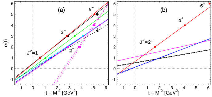
Figure 3: Regge trajectories: (a) $\rho$ black, $\omega$ red, $\phi$ blue, $b_{1}$ and $h_{1}$ green, $\rho_{2}$ and $\omega_{2}$ magenta; dashed and dash-dotted magenta lines are $\rho_{2}$ and $\omega_{2}$ of Ref. Anisovich:2002-1 ; Anisovich:2002-2 ; (b) $f_{2}$ red, $\mathbb{P}$ magenta, $\rho f_{2}$ black solid, $\omega f_{2}$ blue dashed, $\rho\mathbb{P}$ black solid, $\omega\mathbb{P}$ black dashed.

Furthermore, trajectories for tensor mesons $\rho_{2}$ and $\omega_{2}$ are shown in the same plot. These mesons, assuming the same masses for both, were predicted in a relativized quark model Godfrey:1985 for two states: $J^{PC}=2^{--}$ with mass of $1.7$ GeV and $J^{PC}=4^{--}$ with mass of $2.34$ GeV. The trajectory drawn through these two points is shown by the magenta line. According to their quantum numbers, the $\rho_{2}$ and $\omega_{2}$ could be good candidates for the $A_{3}$ amplitude in $\pi^{0}$ and $\eta$ photoproduction. However, there is no clear experimental evidence for the existence of these states. They were found in a partial wave analysis of Refs. Anisovich:2002-1 ; Anisovich:2002-2 and result in much steeper trajectories, that are shown in Fig. 3(a) by the dashed magenta line for the $\rho_{2}$ and dash-dotted magenta line for the $\omega_{2}$.

Technically, the t-channel exchange of Regge trajectories is done by replacing the single meson propagator by the following expression

$$\frac{1}{t-M^{2}}\Rightarrow\left(\frac{s}{s_{0}}\right)^{\alpha(t)-1}\;\frac{\pi\,\alpha^{\prime}}{\mbox{sin}[\pi\alpha(t)]}\;\frac{{\cal S}+e^{-i\pi\alpha(t)}}{2}\;\frac{1}{\Gamma(\alpha(t))}\,,$$ (16)

where $M$ is the mass of the Reggeon, $\cal S$ is the signature of the Regge trajectory, and $s_{0}$ is a mass scale factor, commonly set to 1 $GeV^{2}$. The Gamma function $\Gamma(\alpha(t))$ is introduced to suppress additional poles of the propagator.

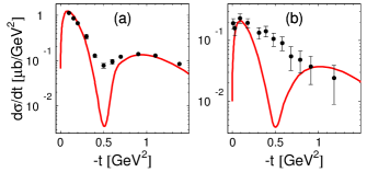
Figure 4: The differential cross sections of $\gamma p\to\pi^{0}p$ (a) and $\gamma p\to\eta p$ (b) reactions at $E_{\gamma}=6$ GeV. Experimental data are from Ref. SLAC:1971 (a) and Ref. DESY:1970 (b). The solid line is a calculation with $\rho$ and $\omega$ exchange in the $t$ channel.

The signature $\cal S$ is determined as ${\cal S}=(-1)^{J}$ for bosons and ${\cal S}=(-1)^{J+1/2}$ for fermions. So ${\cal S}=-1$ for the vector and axial-vector mesons, and ${\cal S}=+1$ for tensor mesons. If ${\cal S}=-1$ and $\alpha(t)=0$, then both, real and imaginary parts, vanish. This results in a characteristic dip of differential cross sections of $\gamma p\to\pi^{0}p$ and $\gamma p\to\eta p$ reactions at $t\approx-0.5$ GeV², which is not observed in experimental data, see Fig. 4.

To avoid problems with the dip at $\alpha(t)=0$, different approaches have been developed, see for example Ref. Nys:2017 ; MAID:2003 ; Sibirtsev:2016 ; Goldstein:1973 ; Barker:1978 ; DoKa:2016 ; Mathieu:2015 . Here we focus on two of them, which are described in the following subsections.

III.3 Regge cuts

Regge cuts were firstly considered in the early work of Refs. Landshoff:1972 ; Goldstein:1973 ; Barker:1978 , where their important role was shown to fill in the dip in the differential cross sections of $\pi^{0}$ and $\eta$ photoproduction. A full discussion of Regge cuts can be found in Ref. Donnachie:2002 . In 2016 Donnachie and Kalashnikova DoKa:2016 revisited the Regge cuts and developed a new approach, where in addition to Regge trajectories of $\rho$, $\omega$, and $b_{1}$ exchange, also Regge cuts from rescattering $\rho{\mathbb{P}}$, $\rho f_{2}$ and $\omega{\mathbb{P}}$, $\omega f_{2}$ were added, where ${\mathbb{P}}$ is the Pomeron with quantum numbers of the vacuum $0^{+}(0^{++})$ and $f_{2}$ is a tensor meson with quantum numbers $0^{+}(2^{++})$. These Regge cuts can be considered as contracted box diagrams, where two particles are exchanged, see Fig. 3(c).

The exchange of two Reggeons with linear trajectories

$$\alpha_{i}(t)=\alpha_{i}(0)+\alpha_{i}^{\prime}t,\quad i=1,2$$ (17)

yields a cut with a linear trajectory $\alpha_{c}(t)$ Landshoff:1972

$$\alpha_{c}(t)=\alpha_{c}(0)+\alpha_{c}^{\prime}\,t\,,$$ (18)

where

$$\alpha_{c}(0) = \alpha_{1}(0)+\alpha_{2}(0)-1\,,$$

$$\alpha_{c}^{\prime} = \frac{\alpha_{1}^{\prime}\alpha_{2}^{\prime}}{\alpha_{1}^{\prime}+\alpha_{2}^{\prime}}\,.$$ (19)

The trajectories for $f_{2}$ and ${\mathbb{P}}$ are shown in Fig 3(b) together with four cut trajectories $\rho{\mathbb{P}}$, $\omega{\mathbb{P}}$ (black solid and dashed lines) and $\rho f_{2}$, $\omega f_{2}$ (blue solid and dashed lines) calculated by Eqs. (17,18,III.3). Parameters of the Reggeon and cut trajectories used in the present work are collected in Table 2.

Table 2: The Reggeon and cut trajectories used in the present work.

Reggeon or cut	$\alpha(t)$
$\rho$	$0.477+0.885\,t$
$\omega$	$0.434+0.923\,t$
$b_{1}$, $h_{1}$,	$-0.013+0.664\,t$
$\rho_{2}$, $\omega_{2}$	$-0.235+0.774\,t$
$f_{2}$,	$0.671+0.817\,t$
$\mathbb{P}$	$1.08+0.25\,t$
$\rho f_{2}$	$0.148+0.425\,t$
$\omega f_{2}$	$0.106+0.436\,t$
$\rho\mathbb{P}$	$0.557+0.195\,t$
$\omega\mathbb{P}$	$0.514+0.197\,t$

All four Regge cuts can contribute to vector and axial vector exchanges and can be written in the following form

$$D_{cut}=\left(\frac{s}{s_{0}}\right)^{\alpha_{c}(t)-1}\;e^{-i\pi\alpha_{c}(t)/2}\;e^{d_{c}t}\,.$$ (20)

In total, the vector meson propagators are replaced by

$$D_{V}={D}_{V}+c_{V\mathbb{P}}\,{D}_{V\mathbb{P}}+c_{Vf_{2}}\,D_{Vf_{2}},\;V=\rho,\omega$$ (21)

and the axial vector meson propagators are replaced by

$$D_{A}={D}_{A}+\sum_{V=\rho,\omega}({\tilde{c}}_{V\mathbb{P}}\,{D}_{V\mathbb{P}}+{\tilde{c}}_{Vf_{2}}\,D_{Vf_{2}}),\;A=b_{1},h_{1}\,,$$ (22)

where the coefficients $c_{V\mathbb{P}},c_{Vf_{2}}$ are for natural parity cuts and ${\tilde{c}}_{V\mathbb{P}},{\tilde{c}}_{Vf_{2}}$ for un-natural parity cuts and are obtained by a fit to the data.

Table 3: Vector and axial vector contributions to invariant amplitudes.

$\eta$	$J^{P}$	Dirac coupling	Invariant amplitudes	Reggeons and cuts
natural	$1^{-},3^{-},\ldots$	$g_{V}^{v}\gamma^{\mu}$	$A_{4}$	$\rho,\omega,\rho{\mathbb{P}},\omega{\mathbb{P}},\rho f_{2},\omega f_{2}$
natural	$1^{-},3^{-},\ldots$	$g_{V}^{\mathfrak{t}}\sigma^{\mu\nu}$	$A_{1}$	$\rho,\omega,\rho{\mathbb{P}},\omega{\mathbb{P}},\rho f_{2},\omega f_{2}$
un-natural	$2^{-},4^{-}\ldots$	$g_{A}^{v}\gamma^{\mu}\gamma_{5}$	$A_{3}$	$\rho_{2},\omega_{2},\rho f_{2},\omega f_{2}$
un-natural	$1^{+},3^{+},\ldots$	$g_{A}^{\mathfrak{t}}\sigma^{\mu\nu}\gamma_{5}$	$A_{2}^{\prime}$	$b_{1},h_{1},\rho f_{2},\omega f_{2}$

In detail, the invariant amplitudes will be changed in the following way

$$\begin{split}\lambda_{\rho}\,g_{\rho}^{v,\mathfrak{t}}\;\frac{1}{t-M_{\rho}^{2}}&\rightarrow\lambda_{\rho}\,g_{\rho}^{v,\mathfrak{t}}\\ &[D_{\rho}(s,t)+c_{\rho\mathbb{P}}\,D_{\rho\mathbb{P}}(s,t)+c_{\rho f}\,D_{\rho f}(s,t)]\,,\\ \lambda_{\omega}\,g_{\omega}^{v,\mathfrak{t}}\;\frac{1}{t-M_{\omega}^{2}}&\rightarrow\lambda_{\omega}\,g_{\omega}^{v,\mathfrak{t}}\\ &[D_{\omega}(s,t)+c_{\omega\mathbb{P}}\,D_{\omega\mathbb{P}}(s,t)+c_{\omega f}\,D_{\omega f}(s,t)]\,,\\ \lambda_{b_{1}}\,g_{b_{1}}^{\mathfrak{t}}\;\frac{1}{t-M_{b_{1}}^{2}}&\rightarrow\lambda_{b_{1}}\,g_{b_{1}}^{\mathfrak{t}}D_{b_{1}}(s,t)\\ &+\lambda_{\rho}\,g_{\rho}^{\mathfrak{t}}\,[{\tilde{c}}_{\rho\mathbb{P}}\,D_{\rho\mathbb{P}}(s,t)+{\tilde{c}}_{\rho f_{2}}\,D_{\rho f_{2}}(s,t)]\\ &+\,\lambda_{\omega}\,g_{\omega}^{\mathfrak{t}}\,[{\tilde{c}}_{\omega\mathbb{P}}\,D_{\omega\mathbb{P}}(s,t)+{\tilde{c}}_{\omega f_{2}}\,D_{\omega f_{2}}(s,t)]\,.\end{split}$$ (23)

In practical calculations, it turns out that the axial vector Regge pole contributions, proportional to $D_{A}$, can be neglected, but the axial vector Regge cuts arising from $\rho$ and $\omega$ together with $\mathbb{P}$ and $f_{2}$ are very important, in particular for polarization observables, as the photon beam asymmetry $\Sigma$.

The Regge cuts also allow us to describe a long standing problem of suitable candidates for an $A_{3}$ amplitude: $\rho f_{2}$ and $\omega f_{2}$ satisfy all conservation law requirements. In Table 3 details of the invariant amplitude structure of the $t$-channel exchanges are given. Here, $\eta$ is a naturality, determined as $\eta=P(-1)^{J}$. For the $\rho{\mathbb{P}}$ and $\omega{\mathbb{P}}$ cuts, $\eta=+1$ and these cuts do not contribute to the $A_{3}$ amplitude. Therefore, we set the coefficients ${\tilde{c}}_{\rho\mathbb{P}}$ and ${\tilde{c}}_{\omega\mathbb{P}}$ in Eq. (23) equal to zero.

Table 4: Coupling constants for $\pi^{0}$ and $\eta$ photoproduction used in Fit I as fixed values.

Reggeon	$\lambda_{\pi^{0}\gamma}$	$\lambda_{\eta\gamma}$	$g^{v}$	$g^{\mathfrak{t}}$
$\rho$	0.115	0.910	2.7	4.2
$\omega$	0.310	0.246	14.2	0.
$b_{1}$	0.091	0.1	0.	-7.6

Table 5: Parameter values obtained from Fit I and Fit III for $\pi^{0}$ and $\eta$ photoproduction.

Solution	Reaction	$c_{\rho\mathbb{P}}$	$c_{\omega\mathbb{P}}$	$c_{\rho f_{2}}$	$c_{\omega f_{2}}$	${\tilde{c}}_{\rho\mathbb{P}}$	${\tilde{c}}_{\omega\mathbb{P}}$	${\tilde{c}}_{\rho f_{2}}$	${\tilde{c}}_{\omega f_{2}}$	$d_{\rho\mathbb{P}}$	$d_{\omega\mathbb{P}}$	$d_{\rho f_{2}}$	$d_{\omega f_{2}}$
I	$\gamma p\to\pi^{0}p$	$0.52$	$-0.06$	$0.72$	$2.98$	$0$	$0$	$-0.65$	$0.007$	$1.07$	$0.37$	$0.62$	$5.02$
		$\pm 0.08$	$\pm 0.01$	$\pm 0.64$	$\pm 0.49$	-	-	$\pm 0.26$	$\pm 0.1$	$\pm 0.71$	$\pm 0.14$	$\pm 0.43$	$\pm 0.77$
I	$\gamma p\to\eta p$	$-2.27$	$0.016$	$5.89$	$-5.96$	$0$	$0$	$-0.18$	$0.25$	$5.5$	$5.5$	$2.36$	$2.36$
		$\pm 0.92$	$\pm 0.09$	$\pm 0.81$	$\pm 0.83$	-	-	$\pm 0.28$	$\pm 0.37$	$\pm 2.1$	-	$\pm 0.19$	-
III	$\gamma p\to\pi^{0}p$	$-0.49$	$0.23$	$1.08$	$2.25$	$0$	$0$	$0.24$	$0.08$	$0.66$	$9.9$	$0.001$	$4.16$
		$\pm 0.09$	$\pm 0.01$	$\pm 0.84$	$\pm 0.32$	-	-	$\pm 0.31$	$\pm 0.1$	$\pm 0.16$	$\pm 0.61$	$\pm 0.87$	$\pm 0.51$
III	$\gamma p\to\eta p$	$-2.59$	$-0.25$	$6.51$	$-5.77$	$0$	$0$	$-0.17$	$-0.13$	$5.5$	$5.5$	$2.49$	$2.49$
		$\pm 0.83$	$\pm 0.31$	$\pm 0.79$	$\pm 0.85$	-	-	$\pm 0.33$	$\pm 0.39$	$\pm 4.4$	-	$\pm 0.18$	-

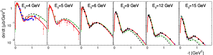
Figure 5: Differential cross sections for $\gamma p\to\pi^{0}p$. The solid red, dashed black, dash-dotted blue (coincide mostly with red curves), and dotted green lines are our solutions I, II, III, and IV, respectively. Data are from SLAC SLAC:1971 (black circles) and from DESY: DESY:1968 (red triangles) and DESY:1973 (blue squares).

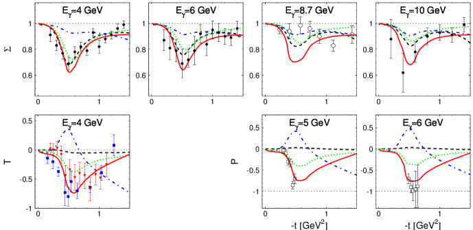
Figure 6: Polarization observables $\Sigma$, $T$, and $P$ for $\gamma p\to\pi^{0}p$. The notation of the lines is the same as in Fig. 5. Data: SLAC SLAC:1971 (black disks), GlueX-17 GlueX:2017 (black open circles), Daresbury Dares:1972 (red triangles), DESY DESY-T:1973 (blue full squares), CEA CEA:1972 (blue open squares).

III.4 Regge amplitudes and fixed-$t$ dispersion relations

The formulation of Regge amplitudes as given in the Section III (B) does not satisfy fixed-$t$ dispersion relations. The reason is mainly given by the ansatz in Eq. (16), where the energy dependence is proportional to $s^{(\alpha(t)-1)}$, violating crossing symmetry. As an alternative ansatz we also used the parametrization of Ref. Nys:2017 (JPAC model)

$$D_{V,A}=-\beta_{i}(t)\;\frac{\pi\,\alpha^{\prime}_{V,A}(e^{-i\pi\alpha_{V,A}(t)}-1)}{2\,\mbox{sin}[\pi\alpha_{V,A}(t)]}\;\left({r_{i}}^{V,A}\nu\right)^{\alpha_{V,A}(t)-1}\,.$$ (24)

Here the Mandelstam variable $s$ is replaced by the crossing variable $\nu$ and the Gamma function in the denominator of Eq. (16) is replaced by a more general residue $\beta_{i}(t)$, where $i=1,2,3,4$ is index of the invariant amplitudes. ${r_{i}}^{V,A}$ are scale parameters of dimension GeV^-1. Each exchange, V or A, has its own scale parameter.

In Ref. Nys:2017 the following residues for $V=\rho,\omega$ and $A=b,h$ are given

$$\beta^{V}_{1}(t) = g^{V}_{1}\,t\,\frac{-\pi\alpha^{\prime V}}{2}\frac{1}{\Gamma(\alpha^{V}(t)+1)}\,,$$ (25)

$$\beta^{V}_{4}(t) = g^{V}_{4}\frac{-\pi\alpha^{\prime V}}{2}\frac{1}{\Gamma(\alpha^{V}(t))}\,,$$ (26)

$$\beta^{\prime A}_{2}(t) = g^{A}_{2}\,t\,\frac{-\pi\alpha^{\prime A}}{2}\frac{1}{\Gamma(\alpha^{A}(t)+1)}\,,$$ (27)

where the prime in $\beta_{2}^{\prime}$ denotes the fact that this is the $A_{2}^{\prime}$ residue, which explains the factor of $t$. The factor $-\pi\alpha^{\prime}/2$ ensures the correct on-shell couplings. The functions $1/\Gamma(\alpha+1)$ and $1/\Gamma(\alpha)$ are both equal to $1$ at the pole $\alpha=1$, however they differ in the physical region.

As possible candidates for the $A_{3}$ amplitude, tensor mesons $\rho_{2}$ and $\omega_{2}$ were suggested in Ref. Nys:2017 . The signature for the tensor mesons is equal to +1, so we use the following parametrization for the propagator

$$D_{T}=-\beta_{3}(t)\;\frac{\pi\,\alpha^{\prime}_{T}(e^{-i\pi\alpha_{T}(t)}+1)}{2\,\mbox{sin}[\pi\alpha_{T}(t)]}\;\left({r_{i}}^{V,A}\nu\right)^{\alpha_{T}(t)-1}$$ (28)

with the residue

$$\beta^{T}_{3}(t) = g^{T}_{3}\frac{-\pi\alpha^{\prime T}}{2}\frac{1}{\Gamma(\alpha^{T}(t))}\,,$$ (29)

where a symbol $T$ denotes the tensor meson, $\rho_{2}$ or $\omega_{2}$. Parameters of the trajectories of these mesons are shown in Table 2. Furthermore, we also assume the same contributions to $A_{3}$ from both mesons.

IV Results

We have used the Regge cut and JPAC models for a fit to the available data for $\gamma p\to\pi^{0}p$ and $\gamma p\to\eta p$ at $E_{\gamma}\geq 4$ GeV. The electromagnetic coupling constants for the $\rho$, $\omega$, and $b_{1}$ mesons were fixed according to Table 4. The best fit using Regge cuts is called Solution I.

Table 6: Four solutions using different models and data sets shown in our analysis.

Solution	Line in Figs.	Model	Data set	$\chi^{2}_{red}(\pi)$	$\chi^{2}_{red}(\eta)$
I	solid red	Regge cut	all	1.46	1.25
II	dashed black	JPAC	all	5.59	2.73
III	dash-dotted blue	Regge cut	d$\sigma$/dt + GlueX $\Sigma$	0.92	1.07
IV	dotted green	JPAC+$\phi$	all	4.17	1.86

Table 7: Partial $\chi^{2}$ per data points of $\pi^{0}$ photoproduction for each observable and each laboratory, for the solutions I and III.

Solution	$d\sigma/dt$	$d\sigma/dt$	$d\sigma/dt$	$\Sigma$	$\Sigma$	$T$	$T$	$P$	$R_{np}$	$R_{np}$	$R_{np}$
	SLAC SLAC:1971	DESY DESY:1968	DESY DESY:1973	SLAC SLAC:1971	GlueX GlueX:2017	Dares Dares:1972	DESY DESY-T:1973	CEA CEA:1972	DESY DESY-np:1973	CEA CEA:1971	Cornell Cornell:1973
I	0.27	1.56	14.5	1.05	4.27	1.69	1.26	2.94	3.85	1.71	1.19
III	0.27	1.36	9.30	4.50	1.05	25.8	4.57	46.2	7.82	3.65	2.82

Table 8: Partial $\chi^{2}$ per data points of $\eta$ photoproduction for each observable and each laboratory, for the solutions I and III.

Solution	$d\sigma/dt$	$d\sigma/dt$	$\Sigma$	$T$
	DESY DESY:1970	WLS WLS:1971	GlueX GlueX:2017	Daresbury Dares:1981
I	1.05	0.94	0.44	2.94
III	0.98	0.98	0.26	3.80

As first step in fits with the JPAC approach, we reproduced exactly the results from Ref. Nys:2017 for the differential cross section of the $\gamma p\to\eta p$ reaction. We then added the tensor mesons $\rho_{2}$ and $\omega_{2}$ with electromagnetic couplings fixed to 1 and fitted the model to all available data in $\pi^{0}$ and $\eta$ production. This result is called Solution II.

IV.1 Results on $\pi^{0}$ photoproduction

In the fits we have used the experimental data for the differential cross sections $d\sigma/dt$ from DESY at $E_{\gamma}=4$ GeV DESY:1973 and $E_{\gamma}=4,5,$ and 5.8 GeV DESY:1968 , and SLAC SLAC:1971 at $E_{\gamma}=6,9,12$, and 15 GeV; the polarized-beam asymmetry $\Sigma$ from SLAC SLAC:1971 at $E_{\gamma}=4,6$, and 10 GeV and GlueX GlueX:2017 at $E_{\gamma}=8.7$ GeV; the target asymmetry $T$ from Daresbury Dares:1972 and DESY DESY-T:1973 , both at $E_{\gamma}=4$ GeV; the recoil polarization observable $P$ from CEA CEA:1972 at $E_{\gamma}=4.1-6.3$ GeV; the differential cross section ratio of neutrons and protons, $R_{np}$ for $\pi^{0}$ photoproduction at $E_{\gamma}=4$  GeV DESY-np:1973 ; CEA:1971 and $E_{\gamma}=4.7$ and 8.2 GeV Cornell:1973 .

The fit results, together with the experimental data, are presented in Fig. 5 for the differential cross sections, in Fig. 6 for the polarization observables, and in Fig. 7 for the ratio $R_{np}$. The data for the recoil polarization observable $P$ are divided in two groups and are shown on panel $E_{\gamma}=5$ GeV for $E_{\gamma}=4.5-5.5$ GeV and on panel $E_{\gamma}$= 6 GeV for $E_{\gamma}=5.5-6.3$ GeV. The best fit with reduced $\chi^{2}_{red}=1.46$ using the Regge cut model is shown by the red lines (Solution I). This solution describes practically all experimental data except the beam asymmetry $\Sigma$ at $E_{\gamma}=8.7$ GeV GlueX:2017 very well. The old data from SLAC SLAC:1971 for $\Sigma$ at $E_{\gamma}=6$ and 10 GeV show a clear dip at $t=-0.5$ GeV². Surprisingly, such a structure is missing for the intermediate energy of 8.7 GeV in the new GlueX data GlueX:2017 . Therefore, we also performed an alternative fit using the Regge cut model without the old polarization data and obtained the Solution III with $\chi^{2}_{red}=0.92$, which is shown in Figs. 5, 6, 7 by the dash-dotted blue line. This solution can describe the GlueX data quite well, but it is absolutely wrong for $T$ and $P$ and also underestimates the old data for $\Sigma$. Therefore, we conclude, that a strong energy dependence of the beam asymmetry between 6 and 10 GeV, as suggested by the GlueX data, cannot be described within our model without adding additional dynamics. There is also some disagreement between the data and the Solution I for the differential cross sections at $E_{\gamma}=4$ GeV, see Figs. 5 and 7. This energy corresponds to the center-of-mass energy $W=2.9$ GeV, that is close to the resonance region. Probably, tails from the resonance contributions still show up in this energy region for $\pi^{0}$ photoproduction and should be take into account.

The central values of the fit parameters for the Solution I and III are shown in Table V together with associated uncertainties. Parameters without errors were fixed in the fits. The coefficients ${\tilde{c}}_{\rho\mathbb{P}}$ and ${\tilde{c}}_{\omega\mathbb{P}}$ are zero because the corresponding terms for the $\rho\mathbb{P}$ and $\omega\mathbb{P}$ cuts do not contribute to the $A_{3}$ amplitude, see Table III. There are also two parameters for the $\gamma p\to\eta p$ reaction that were fixed by empirical constraints: $d_{\omega\mathbb{P}}$ = $d_{\rho\mathbb{P}}$ and $d_{\omega f_{2}}$ = $d_{\rho f_{2}}$.

The best fit with the JPAC model has $\chi^{2}_{red}=5.59$ (Solution II), see black dashed lines in Figs. 5, 6. It describes well the shape of the differential cross sections but has the wrong energy dependence after the dip location, $-t>0.4$ GeV². Similar to the Regge cut solution, it does not describe the new GlueX data for $\Sigma$. Furthermore, the existing data on the polarization observables $T$ and $P$ cannot be described. The inclusion of the exotic tensor mesons $\rho_{2}$ and $\omega_{2}$ did not improve our fits and we did not consider them in our four solutions.

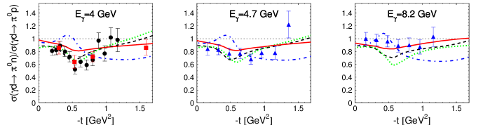
Figure 7: Ratio of differential cross sections for $\pi^{0}$ photoproduction on neutrons and protons. The notation of the lines is the same as in Fig. 5. Data: DESY DESY-np:1973 (black circles), CEA CEA:1971 (red squares), and Cornell Cornell:1973 (blue triangles).

We then investigated the possibility of improving the fit by including the $\phi$ meson in the JPAC model even though small couplings to the nucleon can be expected as discussed above. The electromagnetic coupling constants $\lambda_{\phi\pi^{0}\gamma}$= 0.018 and $\lambda_{\phi\eta\gamma}$= 0.38 are obtained from the corresponding widths $\Gamma_{\phi\rightarrow\pi^{0}\gamma}=5.4\ \mathrm{keV}$ and $\Gamma_{\phi\rightarrow\eta\gamma}=55.84\ \mathrm{keV}$ PDG2016 using Eq. (14). This solution IV is shown in Figs. 5, 6, 7 by the green dotted lines. We did not use $\rho_{2}$ and $\omega_{2}$ for this fit because of their negligible contributions. Indeed, Solution IV describes the polarization observables $T$ and $P$ significantly better than Solution II. The hadronic vector $g^{v}=-4.3$ and tensor $g^{t}=-0.08$ coupling constants for $\phi$ meson were obtained from this fit which we consider as reasonable. A comparison of $\chi^{2}_{red}$ for the different solutions is shown in Table VI.

Table VII gives partial $\chi^{2}$ divided by the number of the data points for each observable and each laboratory, for the solutions I and III.

IV.2 Results on $\eta$ photoproduction

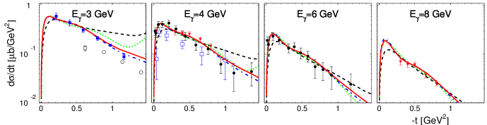
Figure 8: Differential cross sections for $\gamma p\to\eta p$. The notation of the lines is the same as in Fig. 5. Data: DESY DESY:1970 (black disks), WLS WLS:1971 (red triangles), Daresbury Dares:1976 (blue full squares), CLAS CLAS:2009 (black open circles), and CEA CEA:1968 (blue open squares).

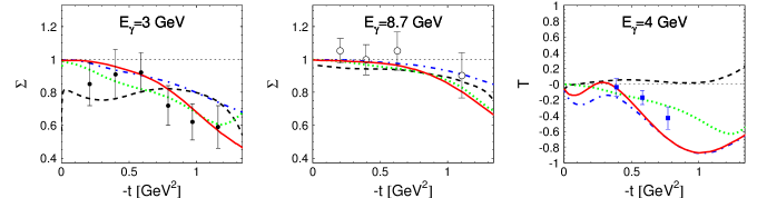
Figure 9: Polarization observables $\Sigma$ and $T$ for $\gamma p\to\eta p$. The notation of the lines is the same as in Fig. 5. Data: GlueX GlueX:2017 (black open circles) and Daresbury: Dares:1976 (black disks) and Dares:1981 (blue squares).

The data set for the $\gamma p\to\eta p$ reaction at high energies is more limited than for $\pi^{0}$ photoproduction. For the fit, we have used the experimental data of the differential cross sections $d\sigma/dt$ from DESY DESY:1970 at $E_{\gamma}$= 4 and 6 GeV and WLS WLS:1971 at $E_{\gamma}$= 4 and 8 GeV; for the polarized-beam asymmetry $\Sigma$ from GlueX GlueX:2017 at $E_{\gamma}=8.7$ GeV; and for the target asymmetry $T$ from Daresbury Dares:1981 .

Our fit results for the differential cross sections are presented in Fig. 8 and for the polarization observables $\Sigma$ and $T$ in Fig. 9. The data for $d\sigma/dt$ and $\Sigma$ at $E_{\gamma}=3$ GeV were not included in the fit, because these are very close to the resonance region. However, the predictions of all our solutions can reproduce also these data quite well. Presumably, the influence of the resonances for $\eta$ photoproduction is already negligible at these energies. Our extrapolation of the differential cross section to $E_{\gamma}=3$ GeV is in good agreement with Ref. Sibirtsev3 .

The best fit with $\chi^{2}_{red}$= 1.25 using the Regge cut model is shown by the solid red line (Solution I). This solution well describes all experimental data including the beam asymmetry $\Sigma$ at $E_{\gamma}=8.7$ GeV GlueX:2017 . The alternative fit without data for $T$, Solution III, also gives a good prediction for this observable.

Table VIII gives partial $\chi^{2}$ divided by the number of the data points for each observable and each laboratory, similar as in Table VII, but for $\eta$ photoproduction.

The fit with the JPAC model has a $\chi^{2}_{red}=2.73$ (Solution II), see dashed black lines in Figs. 8,9. Similar as for $\pi^{0}$ photoproduction, it well describes the differential cross section and $\Sigma$, but contradicts the data for $T$. As in case of $\pi^{0}$ production, the inclusion of the $\phi$ meson (Solution IV), improves the description significantly at low $t$. However, a main drawback of Solution IV is a large overestimation of the total cross section at energies $E_{\gamma}>2$ GeV. Therefore, this solution can not be used as a non-resonant background for partial wave analyses in the resonance region.

IV.3 Further results for high energies

From high-energy approximations of the observables the following relation between the target and recoil polarization to the photon beam asymmetry can be derived in a model independent way (see appendix):

$$|P-T|\leq 1-\Sigma$$ (30)

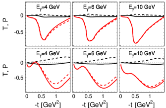
Figure 10: Comparison of the polarization observables $T$ and $P$ at different photon beam energies for $\gamma p\to\pi^{0}p$ (top panels) and for $\gamma p\to\eta p$ (bottom panels). The solid red and black lines are our solutions I and II for the target polarization $T$ and the dashed red and black lines for the recoil polarization $P$, respectively.

As the beam asymmetry $\Sigma$ is almost unity, except in the neighborhood of the dip near $t=-0.5$ GeV², the polarization observables $T$ and $P$ should be almost equal. Any difference between $T$ and $P$ should be due to an interference between the $A_{2}^{\prime}$ and $A_{3}$ amplitudes at high energies, see Eqs. (C3),(C4) in Appendix C. A comparison between $T$ and $P$ for the Solutions I and II is shown in Fig. 10. The Solution I for $\pi^{0}$ photoproduction verifies well this prediction. There is some visible difference between $T$ and $P$ for $\eta$ photoproduction, but in this case no $P$ data were included in the fit.

V Summary and conclusions

Photoproduction $\pi^{0}$ and $\eta$ mesons on the nucleon at photon beam energies above 4 GeV was investigated within two different Regge model approaches. The models include $t$-channel exchange of vector ($\rho$ and $\omega$) and axial vector ($b_{1}$ and $h_{1}$) mesons. Moreover, Regge cuts of $\rho{\mathbb{P}}$, $\rho f_{2}$, $\omega{\mathbb{P}}$, and $\omega f_{2}$ are used. Both models can describe differential cross sections and photon beam asymmetries $\Sigma$ very well, except for a possible strong energy dependence of $\Sigma$ in $\gamma p\to\pi^{0}p$ between 6 and 10 GeV as suggested by recent GlueX data. Within our approach we can not find a solution that can simultaneously describe both the old polarization data and the new GlueX data.

The crossing-odd amplitude $A_{3}$ gets no contributions from dominant $t$-channel vector meson exchange terms. We found possible contributions from tensor meson exchanges and also from Regge cuts. All of them turn out to be rather small. The effect could be worked out in the difference between target and recoil polarizations, but from existing data in $\pi^{0}$ photoproduction no evidence can be seen.

Finally, with the present database only the Regge cut model (Solution I) is able to describe all other available polarization observables as well. However, since most data go back to the late 1960s and early 1970s, and on the other hand new data are in progress, a reliable conclusion can not yet be drawn. For our applications in forthcoming baryon resonance analyses from pseudoscalar meson photoproduction data, we currently favor an extrapolation of Solution I to lower energies as a good description for the non-resonant background.

Appendix A Observables in terms of CGLN amplitudes

Here the polarization observables involving beam and target polarization are expressed by helicity amplitudes in the notation of Barker Barker and Walker Walker . A phase space factor $|{\mathbb{q}}|/|{\mathbb{k}}|$ has been omitted in all expressions. The differential cross section is given by $\sigma_{0}$ and the spin observables $\check{O}_{i}$ are obtained from the spin asymmetries $A_{i}$ by $\hat{O}_{i}=A_{i}\,\sigma_{0}$:

$$\begin{split}\sigma_{0}=&\mbox{Re}\,[{F}_{1}^{*}{F}_{1}+{F}_{2}^{*}{F}_{2}+\sin^{2}\theta\,({F}_{3}^{*}{F}_{3}/2+{F}_{4}^{*}{F}_{4}/2\\ &+{F}_{2}^{*}{F}_{3}+{F}_{1}^{*}{F}_{4}+\cos\theta\,{F}_{3}^{*}{F}_{4})-2\cos\theta\,{F}_{1}^{*}{F}_{2}]\,,\\ \check{\Sigma}=&-\sin^{2}\theta\;\mbox{Re}\,[({F}_{3}^{*}{F}_{3}+{F}_{4}^{*}{F}_{4})/2+{F}_{2}^{*}{F}_{3}+{F}_{1}^{*}{F}_{4}\\ &+\cos\theta\,{F}_{3}^{*}{F}_{4}]\,,\\ \check{T}=&\sin\theta\;\mbox{Im}\,[{F}_{1}^{*}{F}_{3}-{F}_{2}^{*}{F}_{4}+\cos\theta\,({F}_{1}^{*}{F}_{4}-{F}_{2}^{*}{F}_{3})\\ &-\sin^{2}\theta\,{F}_{3}^{*}{F}_{4}]\,,\\ \check{P}=&-\sin\theta\;\mbox{Im}\,[2{F}_{1}^{*}{F}_{2}+{F}_{1}^{*}{F}_{3}-{F}_{2}^{*}{F}_{4}\\ &-\cos\theta\,({F}_{2}^{*}{F}_{3}-{F}_{1}^{*}{F}_{4})-\sin^{2}\theta\,{F}_{3}^{*}{F}_{4}]\,,\\ \check{E}=&\mbox{Re}\,[{F}_{1}^{*}{F}_{1}+{F}_{2}^{*}{F}_{2}-2\cos\theta\,{F}_{1}^{*}{F}_{2}\\ &+\sin^{2}\theta\,({F}_{2}^{*}{F}_{3}+{F}_{1}^{*}{F}_{4})]\,,\\ \check{F}=&\sin\theta\;\mbox{Re}\,[{F}_{1}^{*}{F}_{3}-{F}_{2}^{*}{F}_{4}-\cos\theta\,({F}_{2}^{*}{F}_{3}-{F}_{1}^{*}{F}_{4})]\,,\\ \check{G}=&\sin^{2}\theta\;\mbox{Im}\,[{F}_{2}^{*}{F}_{3}+{F}_{1}^{*}{F}_{4}]\,,\\ \check{H}=&\sin\theta\;\mbox{Im}\,[2{F}_{1}^{*}{F}_{2}+{F}_{1}^{*}{F}_{3}-{F}_{2}^{*}{F}_{4}\\ &+\cos\theta\,({F}_{1}^{*}{F}_{4}-{F}_{2}^{*}{F}_{3})]\,.\\ \end{split}$$

Appendix B CGLN amplitudes in terms of invariant amplitudes

The CGLN amplitudes are obtained from the invariant amplitudes $A_{i}$ by the following equations Dennery:1961 ; Ber:1967 :

$$\begin{split}{F}_{1}=&\frac{W-M_{N}}{8\pi\,W}\,\sqrt{(E_{i}+M_{N})(E_{f}+M_{N})}\big{[}A_{1}\\ &+(W-M_{N})\,A_{4}-\frac{2M_{N}\nu_{B}}{W-M_{N}}\,(A_{3}-A_{4})\big{]}\,,\\ {F}_{2}=&\frac{W+M_{N}}{8\pi\,W}\,|{\mathbb{q}}|\,\sqrt{\frac{E_{i}-M_{N}}{E_{f}+M_{N}}}\big{[}-A_{1}+(W+M_{N})\,A_{4}\\ &-\frac{2M_{N}\nu_{B}}{W+M_{N}}\,(A_{3}-A_{4})\big{]}\,,\\ {F}_{3}=&\frac{W+M_{N}}{8\pi\,W}\,|{\mathbb{q}}|\,\sqrt{(E_{i}-M_{N})(E_{f}+M_{N})}\big{[}(W-M_{N})\,A_{2}\\ &+A_{3}-A_{4}\big{]}\,,\\ {F}_{4}=&\frac{W-M_{N}}{8\pi\,W}\,{\mathbb{q}}^{2}\,\sqrt{\frac{E_{i}+M_{N}}{E_{f}+M_{N}}}\big{[}-(W+M_{N})\,A_{2}\\ &+A_{3}-A_{4}\big{]}\,,\end{split}$$

with $\nu_{B}=(t-\mu^{2})/(4M_{N})$.

Appendix C Observables in terms of invariant amplitudes

For high energies, the polarization observables can conveniently be described in terms of invariant amplitudes. Here we follow Ref. Mathieu:2015 and derive the expressions at leading order in the energy squared:

$$\frac{d\sigma}{dt} \approx \frac{1}{32\pi}\left[|A_{1}|^{2}+|A_{2}^{\prime}|^{2}-t|A_{3}|^{2}-t|A_{4}|^{2}\right]\,,$$ (31)

$$\Sigma\frac{d\sigma}{dt} \approx \frac{1}{32\pi}\left[|A_{1}|^{2}-|A_{2}^{\prime}|^{2}+t|A_{3}|^{2}-t|A_{4}|^{2}\right]\,,$$ (32)

$$T\frac{d\sigma}{dt} \approx \frac{1}{16\pi}\sqrt{-t}\;\text{Im}\left[A_{1}\,A_{4}^{*}-A_{2}^{\prime}\,A_{3}^{*}\right]\,,$$ (33)

$$P\frac{d\sigma}{dt} \approx \frac{1}{16\pi}\sqrt{-t}\;\text{Im}\left[A_{1}\,A_{4}^{*}+A_{2}^{\prime}\,A_{3}^{*}\right]\,.$$ (34)

From these relations, a restriction for the difference between target and recoil polarization can be found

$$|P-T|\leq 1-\Sigma\,.$$ (35)

References

- (1) V. Crede and W. Roberts, Rept. Prog. Phys. 76, 076301 (2013).
- (2) A. C. Irving and R. P. Worden, Phys. Rept. 34, 117 (1977).
- (3) W. Braunschweig et al., Phys. Lett. B 33, 236 (1970).
- (4) W. Braunschweig et al., Nucl. Phys. B 51, 167 (1973).
- (5) M. Braunschweig, W. Braunschweig, D. Husmann, K. Lübelsmeyer, D. Schmitz, Phys. Lett. B 26, 405 (1968).
- (6) R. L. Anderson et al., Phys. Rev. D 4, 1937 (1971).
- (7) H. Al Ghou et al. [GlueX Collaboration], Phys. Rev. C 95, 042201(R) (2017).
- (8) I. G. Aznauryan, Phys. Rev. C 67, 015209 (2003)
- (9) I. G. Aznauryan, Phys. Rev. C 68, 065204 (2003).
- (10) B. Pasquini, D. Drechsel and L. Tiator, Eur. Phys. J. A 27, 231 (2006).
- (11) B. Pasquini, D. Drechsel and L. Tiator, Eur. Phys. J. A 34, 387 (2007).
- (12) R. Dolen, D. Horn and C. Schmid, Phys. Rev. 166, 1768 (1968).
- (13) V. Mathieu, I. V. Danilkin, C. Fernández-Ramírez, M. R. Pennington, D. Schott, A. P. Szczepaniak and G. Fox, Phys. Rev. D 92, no. 7, 074004 (2015).
- (14) J. Nys et al. [Joint Physics Analysis Center], Phys. Rev. D 95, 034014 (2017).
- (15) G. F. Chew, M. L. Goldberger, F. E. Low, and Y. Nambu, Phys. Rev. Lett. 106, 1345 (1957).
- (16) W. T. Chiang, S. N. Yang, L. Tiator, M. Vanderhaeghen and D. Drechsel, Phys. Rev. C 68, 045202 (2003).
- (17) M. M. Kaskulov and U. Mosel, Phys. Rev. C 81, 045202 (2010).
- (18) Byunng Geel Yu, Tae Keun Choi, and W. Kim, Phys. Rev. C 83, 025208 (2011).
- (19) C. Patrignani et al. [Particle Data Group], Chin. Phys. C 40, no. 10, 100001 (2016).
- (20) H. Nagahiro, L Roca, and E. Oset, Phys. Rev. D 77, 034017 (2008).
- (21) P. D. B. Collins, An Introduction to Regge theory and High Energy Physics, Cambridge University Press, Cambridge, 1977.
- (22) S. Godfrey and N. Isgur, Phys. Rev. D 32, 189 (1985).
- (23) A. V. Anisovich et al., Phys. Lett. B 542, 8 (2002).
- (24) A. V. Anisovich et al., Phys. Lett. B 542, 19 (2002).
- (25) G. R. Goldstein, J. F. Owens III, Phys. Rev. D 7, 865 (1973).
- (26) I. S. Barker, J. K. Storrow, Nucl. Phys. B 137, 413 (1978).
- (27) A. Sibirtsev, J. Haidenbauer, S. Krewald, U. -G. Meißner, A. W. Thomas, Eur. Phys. J. A 41, 71 (2009).
- (28) A. Donnachie and Y. S. Kalashnikova, Phys. Rev. C 93, 025203 (2016).
- (29) V. Mathieu, G. Fox, A. P. Szczepaniak, Phys. Rev. D 92, 074013 (2015).
- (30) P. V. Landshoff and J .C. Polkinghorne, Phys. Rep. C 5, 1 (1972).
- (31) A. Donnachie, H. G. Dosch, P. V. Landshoff, and O. Nachtmann. Pomeron Physics and QCD (Cambridge University Press, Cambridge, 2002).
- (32) P. S. L. Booth et al., Phys. Lett. B 38, 339 (1972).
- (33) H. Bienlein et al., Phys. Lett. B 46, 131 (1973).
- (34) M. Deutsch et al., Phys. Rev. Lett. 29, 1752 (1972); Phys. Rev. Lett. 30, 249 (1973).
- (35) W. Braunschweig et al., Nucl. Phys. B 51, 157 (1973).
- (36) G. C. Bolon, D. Bellenger, W. Lobar, D. Luckey, L. S. Osborne, and R. Schwitters, Phys. Rev. Lett. 27, 964 (1971).
- (37) A. M. Osborne, A. Browman, K. Hanson, W. T. Meyer, A. Silverman, F. E. Taylor, and N. Horwitz, Phys. Rev. Lett. 29, 1621 (1972); Phys. Rev. Lett. 30, 814 (1973).
- (38) J. Dewire et al., Phys. Lett. B 37, 326 (1971).
- (39) P. J. Bussey et al., Nucl. Phys. B 185, 269 (1981).
- (40) P. S. L. Booth et al., Phys. Lett. B 61, 479 (1976).
- (41) M. Williams et al., Phys. Rev. C 80, 045213 (2009).
- (42) D. Bellenger et al., Phys. Rev. Lett. 21, 1205 (1968).
- (43) A. Sibirtsev, J. Haidenbauer, S. Krewald, U. -G. Meißner, Eur. Phys. J. A 46, 359 (2010).
- (44) I. S. Barker, A. Donnachie, J. K. Storrow, Nucl. Phys. B 79, 431 (1974).
- (45) R. L. Walker, Phys. Rev. 182, 1729 (1969).
- (46) P. Dennery, Phys. Rev. 124, 2000 (1961).
- (47) F. A. Berends, A. Donnachie, and D. L. Weaver, Nucl. Phys. B 4, 1 (1967).