Non-renewal statistics for electron transport in a molecular junction with electron-vibration interaction

Abstract

Quantum transport of electrons through a molecule is a series of individual electron tunneling events separated by stochastic waiting time intervals. We study the emergence of temporal correlations between successive waiting times for the electron transport in a vibrating molecular junction. Using master equation approach, we compute joint probability distribution for waiting times of two successive tunneling events. We show that the probability distribution is completely reset after each tunneling event if molecular vibrations are thermally equilibrated. If we treat vibrational dynamics exactly without imposing the equilibration constraint, the statistics of electron tunneling events become non-renewal. Non-renewal statistics between two waiting times $\tau_{1}$ and $\tau_{2}$ means that the density matrix of the molecule is not fully renewed after time $\tau_{1}$ and the probability of observing waiting time $\tau_{2}$ for the second electron transfer depends on the previous electron waiting time $\tau_{1}$. The strong electron-vibration coupling is required for the emergence of the non-renewal statistics. We show that in Franck-Condon blockade regime the extremely rare tunneling events become positively correlated.

I Introduction

On the microscopic quantum mechanical level, electron current consists of a sequence of single electron tunneling events separated by random waiting time intervals. Nazarov and Blanter (2009) Statistics of these waiting time intervals reveals the wealth of interesting information about details of quantum transport. Thomas and Flindt (2013); Sothmann (2014); Thomas and Flindt (2014); Potanina and Flindt (2017); Tang et al. (2014); Seoane Souto et al. (2015); Goswami and Harbola (2015); Rudge and Kosov (2016a, b); Kosov (2017) The statistical properties of the waiting times are usually studied using waiting time distribution (WTD), which is a conditional probability distribution that we observe the electron transfer in the detector electrode (drain or source) at time $t+\tau$ given that an electron was detected in the same electrode at time $t$.Brandes (2008) WTD is a complementary to very popular full counting statistics in quantum transport and it has recently gained a significant popularity in the study of nanoscale and mesoscale systems.Albert et al. (2012); Thomas and Flindt (2013); Sothmann (2014); Thomas and Flindt (2014); Dasenbrook et al. (2015); Tang et al. (2014); Seoane Souto et al. (2015); Goswami and Harbola (2015); Rudge and Kosov (2016a, b); Kosov (2017)

The question which we discuss in this paper is the following. When an electron transfers through a molecular junction, is there exists a correlation between waiting times for successive electron tunneling or they are statistically independent? Is it possible to have, for example, a situation, when the second tunneling electron senses the waiting time of the previous electron and changes its own waiting time accordingly? Intuitively, we expect that such kind of statistical temporal correlations can emerge in molecular junctions with strong electron-vibrational coupling – the excitation of a particular vibrational state depends on the waiting time of the electron, and the waiting time for the second electron feels the previous one through this vibration. Strong coupling between electronic and nuclear dynamics distinguishes molecular junctions from other nanoscale quantum transport systems. The interplay between nuclear and electronic dynamics has already led to the discovery of distinctly molecular junction phenomena as Franck-Condon blockade, Koch and von Oppen (2005); Koch et al. (2006); Lau et al. (2016) negative differential resistance, Härtle and Thoss (2011); Kuznetsov (2007); Galperin et al. (2005); Zazunov et al. (2006); Dzhioev and Kosov (2012) nonequilibrium chemical reactions,Dzhioev and Kosov (2011); Thomas et al. (2012); Dzhioev et al. (2013) cooling of nuclear motion by electric current.Galperin et al. (2009); Ioffe et al. (2008); Härtle and Thoss (2011)

The basis for our work is the extension of ideas of WTD beyond studying statistics of single waiting time to the domain of multiple waiting times joint probability distribution.Ptaszyński (2017) Renewal theory assumes that successive waiting times between transport events are statistically independent equally distributed random variables. In this case the joint probability density of two successive waiting times $w_{2}(\tau_{2},\tau_{1})$ can be factorised into a product of two single-time distributions $w_{1}(\tau_{2})w_{1}(\tau_{1})$, that means that the distribution is totally ”renewed” after waiting time $\tau_{1}$. The non-renewal statistics means the existence of temporal correlations between the subsequent tunneling events $w_{2}(\tau_{2},\tau_{1})\neq w_{1}(\tau_{2})w_{1}(\tau_{1})$. The study of non-renewal statistics is a very interesting topic on its own. Although the questions of temporal correlations between electron tunneling events are only started to appear in quantum transport,Ptaszyński (2017); Dasenbrook et al. (2015) the non-renewal statistics has a long history in chemical physics where it was used to describe single-molecule processes in spectroscopyCao (2006); Osad’ko and Fedyanin (2011); Budini (2010); Witkoskie and Cao (2006) and kinetics.Saha et al. (2011); Cao and Silbey (2008)

The paper is organised as follows. Section II overviews the derivation of the master equation for electron transport through a vibrating molecular junction. In Section III, we introduce quantum jump operators and derive the expression for the joint probability density of two successive waiting times, $w_{2}(\tau_{1},\tau_{2})$. Section IV describes the results of numerical and analytical calculations. Section V summarises the main results of the paper.

We use natural units for quantum transport throughout the paper: $\hbar=k_{B}=e=1$.

II Master equation in the polaronic regime

The single-molecular junction is a molecule connected to macroscopic source (S) and drain (D) electrodes. The corresponding Hamiltonian is

$$H=H_{\text{molecule}}+H_{\text{electrodes}}+H_{T}.$$ (1)

The molecule is modelled by Anderson-Holstein model – a single electronic level interacting with a localised vibration. The molecular Hamiltonian is:

$$H_{\text{molecule}}=\epsilon_{0}a^{\dagger}a+\lambda\omega(b^{\dagger}+b)a^{\dagger}a+\omega b^{\dagger}b,$$ (2)

where $\epsilon_{0}$ is molecular orbital energy, $\omega$ is molecular vibration energy, and $\lambda$ is the strength of the electron-vibration coupling. $a^{\dagger}(a)$ creates (annihilates) an electron on molecular orbital, and $b^{+}(b)$ is bosonic creation (annihilation) operator for the molecular vibration. The electronic spin does not play any role here and will not be included explicitly into the equations. Electrodes have noninteracting electrons:

$$H_{\text{electrodes}}=\sum_{k,\alpha=S,D}\epsilon_{k\alpha}a^{\dagger}_{k\alpha}a_{k\alpha},$$ (3)

where $a^{\dagger}_{k\alpha}$ creates an electron in the single-particle state $k$ of the source(drain) electrode $\alpha=S(D)$ and $a_{k\alpha}$ is the corresponding electron annihilation operator. The molecule-electrode coupling is described by tunneling interaction

$$H_{T}=\sum_{k,\alpha=S,D}t_{\alpha}(a^{\dagger}_{k\alpha}a+a^{\dagger}a_{k\alpha}),$$ (4)

where $t_{\alpha}$ is the tunneling matrix element.

Using Born-Markov approximation and Lang-Firsov transormationLang and Firsov (1963) we obtain the master equation Mitra et al. (2004):

$$\dot{P}_{0q}(t) = \sum_{\alpha q^{\prime}}\Gamma^{\alpha}_{0q,1q^{\prime}}P_{1q^{\prime}}(t)-\Gamma^{\alpha}_{1q^{\prime},0q}P_{0q}(t),$$ (5)

$$\dot{P}_{1q}(t) = \sum_{\alpha q^{\prime}}\Gamma^{\alpha}_{1q,0q^{\prime}}P_{0q^{\prime}}(t)-\Gamma^{\alpha}_{0q^{\prime},1q}P_{1q}(t),$$ (6)

where $P_{nq}(t)$ is the probability that the molecule is occupied by $n$ electrons and $q$ vibrational quanta at time $t$. The transition rates rates are:Mitra et al. (2004)

$$\Gamma^{\alpha}_{0q^{\prime},1q}=\gamma^{\alpha}|X_{q^{\prime}q}|^{2}\left(1-f_{\alpha}[\epsilon-\omega(q^{\prime}-q)]\right).$$ (7)

– transition from state occupied by one electron and $q$ vibrations to the electronically unoccupied state with $q^{\prime}$ vibrations by the electron transfer from the molecule to $\alpha=S,D$ electrode and

$$\Gamma^{\alpha}_{1q^{\prime},0q}=\gamma^{\alpha}|X_{q^{\prime}q}|^{2}f_{\alpha}[\epsilon+\omega(q^{\prime}-q)]$$ (8)

– transition when electron is transferred from $\alpha$ electrode into the originally empty molecules simultaneously changing the vibrational state from $q$ to $q^{\prime}$. The rates depend on the occupation of electrodes given by Fermi-Dirac numbers

$$f_{\alpha}(E)=\frac{1}{1+e^{(E-\mu_{\alpha})/T}},$$ (9)

where $T$ is the temperature and $\mu_{\alpha}$ is the chemical potential of the electrode $\alpha$. The rates also depend on the Franck-Condon factor

$$X_{qq^{\prime}}=\langle{q}|\,e^{-\lambda(b^{\dagger}-b)}\,|{q^{\prime}}\rangle,$$ (10)

and the electronic level broadening

$$\gamma^{\alpha}=2\pi t_{\alpha}^{2}\rho_{\alpha}$$ (11)

where $\rho_{\alpha}$ is density of states in the electrode $\alpha$ taken at molecular orbital energy $\epsilon$.

III Quantum jumps operators for electron tunneling and waiting time distributions

We introduce probability vector ordered in such a way that the electronic probabilities enter in pairs for each vibrational states

$$\mathbf{P}(t)=\begin{bmatrix}P_{00}(t)\\ P_{10}(t)\\ {P_{01}(t)}\\ {P_{11}(t)}\\ \vdots\\ {P_{0N}(t)}\\ {P_{1N}(t)}\\ \end{bmatrix},$$ (12)

where $N$ is the total number of vibrational states included into the calculations. We also define the identity vector of length $2N$:

$$\mathbf{I}=\begin{bmatrix}1\\ 1\\ 1\\ 1\\ \vdots\\ 1\\ 1\\ \end{bmatrix}.$$ (13)

The normalisation of the probability is given by the scalar product between $\mathbf{I}$ and $\mathbf{P}$ vectors $(\mathbf{I},\mathbf{P}(t))$

$$(\mathbf{I},\mathbf{P}(t))=\sum_{q=0}^{N}P_{0q}(t)+P_{1q}(t)=1.$$ (14)

Using this probability vector we write the master equation (5,6) in the matrix form

$$\dot{\mathbf{P}}(t)={\cal L}\mathbf{P}(t),$$ (15)

where $\cal L$ is the Liouvillian operator. The quantum jump operator is $2N\times 2N$ matrix which is defined through the actions on the probability vector:Kosov (2017)

$$({J}\mathbf{P}(t))_{mq}=\delta_{m0}\sum_{q^{\prime}}\Gamma^{D}_{0q,1q^{\prime}}P_{1q^{\prime}}(t).$$ (16)

It describes the tunneling of electron from the molecule to the drain electrode.

We assume that the system has reached the nonequilibrium steady state. Therefore it is described by the steady state density matrix, which is the null vector of the full Liouvillian

$${\cal L}\;\mathbf{P}=0.$$ (17)

Let us begin to monitor time delays between sequential quantum tunnelings in the nonequilibrium steady state. WTD for two waiting times, $w_{2}(\tau_{2},\tau_{1})$, is defined as joint probability distribution that the first electron waits time $\tau_{1}$ and the next electron waits time $\tau_{2}$ for the tunneling to the drain electrode

$$w_{2}(\tau_{2},\tau_{1})=(\mathbf{I},\;J\;e^{({\cal L}-J)\tau_{2}}\;J\;e^{({\cal L}-J)\tau_{1}}\;J\;\mathbf{P}).$$ (18)

The definition becomes physically obvious if one reads it from right to left: The system is in the steady state described by the probability vector $\mathbf{P}$, then it undergoes quantum jump $J$, then idle without the quantum jump for time $\tau_{1}$, then again undergoes quantum jump $J$, idle for time $\tau_{2}$ and then experiences the quantum jump $J$. WTD for single waiting time between two consecutive tunneling events is

$$w_{1}(\tau)=(\mathbf{I},\;J\;e^{({\cal L}-J)\tau}\;J\;\mathbf{P}).$$ (19)

and again this definition is quite self-explanatory. Let us normalise these distributions

$$\int_{0}^{\infty}d\tau_{1}\int_{0}^{\infty}d\tau_{2}\;w_{2}(\tau_{2},\tau_{1})$$

$$=(\mathbf{I},\;J\;({\cal L}-J)^{-1}\;J\;({\cal L}-J)^{-1}\;J\;\mathbf{P})$$

$$=(\mathbf{I},\;(J-{\cal L}+{\cal L})\;({\cal L}-J)^{-1}\;J\;({\cal L}-J)^{-1}\;J\;\mathbf{P})$$

$$=-(\mathbf{I},\;J\;({\cal L}-J)^{-1}\;J\;\mathbf{P})$$

$$=-(\mathbf{I},\;(J-{\cal L}+{\cal L})\;({\cal L}-J)^{-1}\;J\;\mathbf{P})$$

$$=(\mathbf{I},\;J\;\mathbf{P}).$$

Here we used that $(\mathbf{I},\;{\cal L}\;\mathbf{X})=0$ for arbitrary vector $\mathbf{X}$. The normalised joint WTD for two waiting time is

$$w_{2}(\tau_{2},\tau_{1})=\frac{(\mathbf{I},\;J\;e^{({\cal L}-J)\tau_{2}}\;J\;e^{({\cal L}-J)\tau_{1}}\;J\;\mathbf{P})}{(\mathbf{I},\;J\;\mathbf{P})}.$$ (20)

The WTD $w_{1}(\tau)$ has the same normalisation (easy to show by computing the integral over $\tau$)Kosov (2017)

$$w_{1}(\tau)=\frac{(\mathbf{I},\;J\;e^{({\cal L}-J)\tau}\;J\;\mathbf{P})}{(\mathbf{I},\;J\;\mathbf{P})}.$$ (21)

The formal derivation of WTDs (20) and (21) is presented in appendix A.

Let us also check that these definitions (20) and (21) are consistent with each other. Integrating $w_{2}$ over the second time yields

$$\int_{0}^{\infty}d\tau_{2}\;w_{2}(\tau_{2},\tau_{1})$$

$$=-\frac{(\mathbf{I},\;J\;({\cal L}-J)^{-1}\;J\;e^{({\cal L}-J)\tau_{1}}\;J\;\mathbf{P})}{(\mathbf{I},\;J\;\mathbf{P})}$$

$$=-\frac{(\mathbf{I},\;(J-{\cal L}+{\cal L})\;({\cal L}-J)^{-1}\;J\;e^{({\cal L}-J)\tau_{1}}\;J\;\mathbf{P})}{(\mathbf{I},\;J\;\mathbf{P})}$$

$$=\frac{(\mathbf{I},\;J\;e^{({\cal L}-J)\tau_{1}}\;J\;\mathbf{P})}{(\mathbf{I},\;J\;\mathbf{P})}=w_{1}(\tau_{1}).$$

Performing integration over the first waiting time (and using ${\cal L}\mathbf{P}=0$) gives

$$\int_{0}^{\infty}d\tau_{1}\;w_{2}(\tau_{2},\tau_{1})$$

$$=-\frac{(\mathbf{I},\;J\;e^{({\cal L}-J)\tau_{2}}\;J\;({\cal L}-J)^{-1}\;J\;\mathbf{P})}{(\mathbf{I},\;J\;\mathbf{P})}$$

$$=-\frac{(\mathbf{I},\;J\;e^{({\cal L}-J)\tau_{2}}\;J\;({\cal L}-J)^{-1}\;(J-{\cal L}+{\cal L})\;\mathbf{P})}{(\mathbf{I},\;J\;\mathbf{P})}$$

$$=\frac{(\mathbf{I},\;J\;e^{({\cal L}-J)\tau_{2}}\;J\;\mathbf{P})}{(\mathbf{I},\;J\;\mathbf{P})}=w_{1}(\tau_{2}).$$

Therefore, our definitions for single and double time WTDs are consistent with each and have clear probabilistic meaning.

To compute higher-order expectation values and analyse the fluctuations, we introduce the cumulant-generating functions for the joint waiting time probability distribution

$$K(x_{1},x_{2})=\int_{0}^{\infty}d\tau_{1}\int_{0}^{\infty}d\tau_{2}\;e^{ix_{1}\tau_{1}}e^{ix_{2}\tau_{2}}w_{2}(\tau_{1},\tau_{2}).$$ (22)

Integrating the cumulant-generating function over $\tau_{1}$ and $\tau_{2}$, we get

$$K(x_{1},x_{2})=\frac{(\mathbf{I},\;J\;G(x_{1})\;J\;G(x_{2})\;J\;\mathbf{P})}{(\mathbf{I},\;J\;\mathbf{P})},$$

where

$$G(x)=({\cal L}-J+ix)^{-1}.$$ (23)

We obtain all possible higher order comulants differentiating $K(x_{1},x_{2})$ with respect to $x_{1}$ and $x_{2}$.

IV Results

IV.1 Equilibrium molecular vibrations

Master equation (5,6) describes the non-equilibrium dynamics of molecular vibrations. Let us first consider the limit where the vibration is maintained in thermodynamic equilibrium at some temperature $T$, which is not necessarily the same as the temperature of electrons in the leads. To implement this limit we use the following separable ansatz for the probabilitiesMitra et al. (2004)

$$P_{nq}(t)=P_{n}(t)\frac{e^{-q\omega/T}}{1-e^{-\omega/T}},$$ (24)

which assumes that the vibration maintains the equilibrium distribution at all time. The master equation (5,6) is reduced to

$$\frac{d}{dt}\left[\begin{array}[]{c}P_{0}\\ P_{1}\end{array}\right] = \left[\begin{array}[]{cc}-\Gamma_{10}&\Gamma_{01}\\ \Gamma_{10}&-\Gamma_{01}\end{array}\right]\left[\begin{array}[]{c}P_{0}\\ P_{1}\end{array}\right],$$

where the vibration averaged rates are defined as

$$\Gamma^{\alpha}_{mn}=\sum_{qq^{\prime}}\Gamma^{\alpha}_{mq,nq^{\prime}}\frac{e^{-q^{\prime}\omega/T}}{1-e^{-\omega/T}}.$$ (26)

Let us identify the quantum jump operator for the electron tunneling from the molecule to the drain electrode. We write this jump operator in matrix form and as a dyadic product of two vectors

$${J}=\left[\begin{array}[]{cc}0&\Gamma_{01}^{D}\\ 0&0\end{array}\right]=\Gamma^{D}_{01}\left[\begin{array}[]{c}1\\ 0\end{array}\right]\left[\begin{array}[]{cc}0&1\end{array}\right].$$ (27)

Then straightforward vector algebra brings the WTD $w_{1}(\tau)$ (21) to the following form

$$w_{1}(\tau)=\Gamma_{01}^{D}\left[\begin{array}[]{cc}0&1\end{array}\right]e^{({\cal L}-J)\tau}\left[\begin{array}[]{c}1\\ 0\end{array}\right].$$ (28)

For WTD $w_{2}(\tau_{1},\tau_{2})$ (20) we have

$$w_{2}(\tau_{2},\tau_{2})=\Gamma_{01}^{D}\left[\begin{array}[]{cc}0&1\end{array}\right]e^{({\cal L}-J)\tau_{2}}\left[\begin{array}[]{c}1\\ 0\end{array}\right]\Gamma_{01}^{D}\left[\begin{array}[]{cc}0&1\end{array}\right]e^{({\cal L}-J)\tau_{1}}\left[\begin{array}[]{c}1\\ 0\end{array}\right]=w_{1}(\tau_{2})w_{1}(\tau_{1}).$$ (29)

We see that $w_{2}$ is always exactly factorised as a product of two independent $w_{1}$. Therefore, if the molecular vibration is held in thermal equilibrium, then the electronic distribution is always fully reset after each tunneling events and there is no correlation between subsequent tunneling electrons.

IV.2 Nonequilibrium molecular vibrations

Let us now turn our attention to the case of fully nonequilibrium dynamics of molecular vibrations. We must rely on the numerical calculations to get answers in this situation.

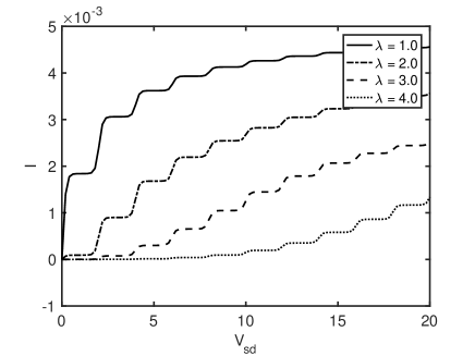
Figure 1: Current $I$ as a function of applied voltage $V_{sd}$. Parameters used in calculations (all energy values are given in units of $\omega$): $\omega=1$,$\gamma_{S}=\gamma_{D}=0.01$, $T=0.05$, $\epsilon=0$. Unit for electric current is $\omega$ (or if we put $\hbar$ and $e$ back, it is $e\omega$) and values of voltage bias $V_{sd}$ are given in $\omega$ (or $\hbar\omega/e$).

We first compute electric current as a function of the applied voltage bias $V_{sd}$. The voltage bias is enforced by shifting symmetrically the chemical potentials of the electrodes $\mu_{S}=V_{sd}/2$ and $\mu_{D}=-V_{sd}/2$. Fig.1 shows the current-voltage characteristics. It has been studied in various details in many works before Galperin et al. (2007); Härtle and Thoss (2011); Cuevas and Scheer (2010) and we show it here simply to serve as a reference - the characteristics steps in the current-voltage characteristic will be related to the behaviour of the waiting time. The steps in the current are due to the resonant excitations of the molecular vibrations by inelastic tunneling of electrons. The steps are observed when the voltage passes through an integer multiple of the vibration energy. We also observe the current suppression in the strong electron-vibration coupling regime due to Franck-Condon blockade.Koch et al. (2006)

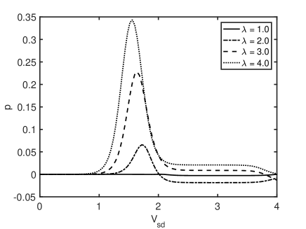
Figure 2: Pearson correlation coefficient between two subsequent tunneling events, $p=(\langle\tau_{1}\tau_{2}\rangle-\langle\tau\rangle^{2})/(\langle\tau^{2}\rangle-\langle\tau\rangle^{2})$ as a function of applied voltage $V_{sd}$ computed for different strengths of electron-vibration coupling. Parameters used in calculations (all energy values are given in units of $\omega$): $\omega=1$, $\gamma_{S}=\gamma_{D}=0.01$, $T=0.05$, $\epsilon=0$. The voltage bias $V_{sd}$ is given in $\omega$.

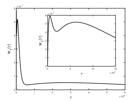
Figure 3: Waiting time distribution $w_{1}(\tau)$ for $\lambda=4$ and $V_{sd}=1.56\omega$. Parameters used in calculations (all energy values are given in units of $\omega$): $\omega=1$, $\gamma_{S}=\gamma_{D}=0.01$, $T=0.05$, $\epsilon=0$. Insert figure zooms the WTD in the short waiting time. Unit for time is $1/\omega$.

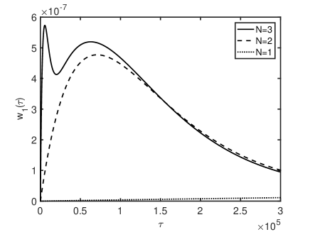
Figure 4: Waiting time distribution $w_{1}(\tau)$ for $\lambda=4$ and $V_{sd}=1.56\omega$ computed for different numbers of vibrational occupation cutoffs. Parameters used in calculations (all energy values are given in units of $\omega$): $\omega=1$, $\gamma_{S}=\gamma_{D}=0.01$, $T=0.05$, $\epsilon=0$. Unit for time is $1/\omega$.

Correlations between two subsequent tunneling events will be measured using Pearson correlation coefficient

$$p=\frac{\langle\tau_{1}\tau_{2}\rangle-\langle\tau\rangle^{2}}{\langle\tau^{2}\rangle-\langle\tau\rangle^{2}}.$$ (30)

Integrals in the Pearson coefficient are computed using cumulant generating function (III): For the correlations we have

$$\langle\tau_{2}\tau_{1}\rangle=\int_{0}^{\infty}d\tau_{1}\int_{0}^{\infty}d\tau_{2}\;\tau_{1}\tau_{2}w_{2}(\tau_{2},\tau_{1})$$

$$=\frac{(\mathbf{I},\;J\;G(0)^{2}\;J\;G(0)^{2}\;J\;\mathbf{P})}{(\mathbf{I},\;J\;\mathbf{P})}$$ (31)

and moments of single waiting time are

$$\langle\tau^{n}\rangle=\int_{0}^{\infty}d\tau_{1}\;\tau^{n}w_{1}(\tau)=n!(-1)^{n+1}\frac{(\mathbf{I},\;J\;G(0)^{n+1}\;J\;\mathbf{P})}{(\mathbf{I},\;J\;\mathbf{P})}.$$ (32)

The Pearson correlation coefficient $p$ is widely used in statistics as a measure of correlations between two stochastic variables. It varies between $-1$ and $+1$: $p=0$ means that there is no correlations, $p>0$ indicates positive correlations, and $p<0$ suggests the variables are anticorrelated (negative correlations). In our case positive correlations mean that if the first waiting time increases/decreases then the waiting time for the second electron also increases/decreases. The negative correlations indicate that if the first electron waits longer then the waiting time for the second electron decreases (and vice versa).

Fig.2 shows the Pearson correlation coefficient between successive electron tunneling events (30) computed as a function of the applied voltage bias for different values of electron-vibration coupling. If there is electron-vibration coupling, then the waiting time for successive electron tunneling are not correlated. The correlation does not appear in the weak and moderate electron-vibration coupling regimes (for $\lambda<1$). Only when the electron-vibrational interaction becomes strong $\lambda>1$, the statistical correlations between electronic tunneling events start to emerge.

We focus on the strong coupling regime ($\lambda=2$, $\lambda=3$ and $\lambda=4$ in Fig.2), this is where the voltage dependence of the Pearson correlation coefficient is very interesting. The tunneling events are positively correlated in the narrow voltage window $\omega\leq V_{sd}\leq 2\omega$ (the negative correlations for $\lambda=2$ all have $p<0.02$ – they are statistically negligible). Comparing Fig.1 and Fig.2, we see positive correlations belong to the Franck-Condon blockade regime where the electric current is small and, therefore, the tunneling events are extremely rare.

Let us understand why the electron tunneling events become suddenly positively correlated. First, we compute WTD $w_{1}(\tau_{1})$ for $\lambda=4$ and $V_{sd}=1.56\;\omega$. The dependence of $w_{1}(\tau_{1})$ on the waiting time is shown in Fig.3. The distribution has a large double peaked spike for the fast electrons (the first narrow peak is barely seen on the main figure since it is very close to the axis) - the structure of the spike is zoomed in the insert of Fig.3. To understand the origin of this behaviour of WTD, we compute waiting time distribution for various cutoffs $N$ for the number of the vibrational quanta included in the calculations (Fig.4). For $N=1$ (it means that only states with vibrational quantum numbers $q=0,1$ are included in the calculations), the short time peaks disappear completely. For $N=2$ (vibrational quantum numbers $q=0,1,2$ are included), the short time WTD spike consists only of the one broad peak. For $N=3$ (vibrational quantum numbers $q=0,1,2,3$ are included), the short time WTD spike forms its final two peak structure. Increasing $N$ further does not affect the short time behaviour of WTD at the considered voltage.

We are now in the position to explain the physical reasons behind the appearance of the positive temporal correlations. The mode of the distribution is the first early time peak - it gives us the waiting time for the electrons most often observed in the transport. These fast travelling electrons are responsible for the emergence of the correlations between successive electron tunneling events. We focus on the regime where we observe positive correlations ($\lambda=4$ and $V_{sd}=1.56\;\omega$). After the first quantum jump the first $q=1$ and second $q=2$ vibrational states become populated in the density matrix (57). Then, if the first waiting time $\tau_{1}$ is around the mode of the waiting time distribution $w_{1}(\tau_{1})$ (Fig.3), the vibrational state $q=3$ is predominantly populated after the waiting time $\tau_{1}$(see the appendix for details). If we look at the absolute values of the first 4 components of the Franck-Condon factor $|X_{qq^{\prime}}|,\;q,q^{\prime}=0,..,3$ computed for $\lambda=4$

$$|X|=\left(\begin{array}[]{cccc}0.0003&0.0013&0.0038&0.0088\\ 0.0013&0.0050&0.0133&0.0285\\ 0.0038&0.0133&0.0325&0.0643\\ 0.0088&0.0285&0.0643&0.1160\end{array}\right)$$ (33)

we see that it creates the ”shortcut” opening the elastic transport channel through the vibrational state $q=3$. This elastic channel opens only for a short time during the first narrow peak in the WTD $w_{1}(\tau)$ (Fig.3). The higher states $q=4,5,...$ have even larger diagonal Franck-Condon factor but they are not populated on the short time scale at this voltage range. At the higher voltages many vibrational states are populated already in the steady state density matrix, but it does not lead to the correlations since too many elastic channels are available anyway irrespective to the previous tunneling electron.

These temporal correlations between tunneling times should not be confused with ”avalanche” electron transport phenomena in molecular junctions with strong electron-vibrational coupling.Koch and von Oppen (2005); Koch et al. (2006); Lau et al. (2016) The ”avalanche” transport of electrons is observed at intermediate voltage range $3\omega<V_{sd}<6\omega$ just after the Franck-Condon plato in I-V characteristics and it does not involve the correlations between different waiting times.Koch and von Oppen (2005) The avalanche electron transport is simply manifestation of the fact that the mode of WTD is much smaller than the average time given by the same distribution.

V Conclusions

In this paper, we developed the theory for computing joint waiting time distribution for electron transport through a molecular junction with strong electron-vibrational interaction. The molecule is modelled by one molecular orbital coupled with a single localised vibration. We treat electron-vibration interaction exactly and molecule-electrode coupling within the Born-Markov approximation. Using this master equation we computed joint waiting time probability distribution and studied it across various transport regimes to understand the emergence and disappearance of the correlations between successive electron tunneling events.

Our main observations are summarised below:

• There are no temporal correlations between subsequent electron tunneling events (the distribution function is completely renewed after each electron tunneling)

  1. for small voltage bias ($<\omega$) and for voltages greater than $2\omega$;

  2. irrespective of voltage bias if electron-vibration coupling $\lambda<1$;

  3. irrespective to voltage and electron-vibration coupling strength if the vibration is maintained in thermodynamic equilibrium.

• The temporal correlations between subsequent electron tunnelings emerge, if $\omega<V_{sd}<2\omega$ and $\lambda>1$. The tunneling events become positively correlated which means that the second electron can sense the waiting time for the first electron and if the first electron was fast, then the second electron also would like to be transferred quickly (and opposite, slow to slow correlations are also possible). The observed results are robust, they do not require any special tuning of the parameters other than the physically reasonable choices of applied voltage and electron-vibration coupling.

• The physical origin of positively correlated waiting times is the following. After the initial electron transfer to the drain electrode the ground and the first excited vibrational states are predominantly populated. Next, if the first waiting time happens to be around the modal time, then the electron has an opportunity to excite the molecule in $q=3$ state via tunneling through inelastic $q=0$ to $q=3$ or $q=1$ to $q=3$ channels. The excitation of $q=3$ vibrational state creates a ”shortcut” between the source and drain electrodes via the elastic channel with large Franck-Condon factor which can be utilised by the next electron. In other words, if the the first waiting time is the modal time (very short), then the tunneling electron opens $q=3$ elastic channel for swift transfer for the next electron (positive correlations).

Appendix A Waiting time distributions for electron detection events

In this appendix, we define WTDs (21) and (20) using methods of quantum measurement theory. Our derivations follow the theory originally developed in quantum optics to study single photon counting statistics Srinivas and Davies (2010); Zoller et al. (1987); Budini (2010) and extended to quantum transport by Brandes.Brandes (2008)

The Liouvillian in the master equation (15) is decomposed as

$$\dot{\mathbf{P}}(t)=({\cal L}_{0}+J)\mathbf{P}(t),$$ (34)

where $J$ is quantum jump operator (16) and ${\cal L}_{0}={\cal L}-J$ generates the evolution of the molecular junction without transferring electrons to the drain electrode. This differential equation is converted to the integral equation

$$\mathbf{P}(t)=e^{{\cal L}_{0}t}\mathbf{P}(0)+\int_{0}^{t}dt_{1}e^{{\cal L}_{0}(t-t_{1})}J\mathbf{P}(t_{1}),$$ (35)

which then is resolved by iterations

$$\mathbf{P}(t)=e^{{\cal L}_{0}t}\mathbf{P}(0)+\int_{0}^{t}dt_{1}e^{{\cal L}_{0}(t-t_{1})}Je^{{\cal L}_{0}t_{1}}\mathbf{P}(0)$$ (36)

$$+\int_{0}^{t}dt_{1}\int_{0}^{t_{1}}dt_{2}e^{{\cal L}_{0}(t-t_{1})}Je^{{\cal L}_{0}(t_{1}-t_{2})}Je^{{\cal L}_{0}t_{2}}\mathbf{P}(0)+....$$

We introduce operator $M$ - it describes detection of electron transfer from the molecule to the drain electrode (quantum measurement operator). If $\mathbf{P}(t)$ is the probability vector before the measurement, then after the electron detection it becomesBreuer and Petruccione (2002)

$$M\mathbf{P}(t)=\frac{J\mathbf{P}(t)}{(\mathbf{I},J\mathbf{P}(t))}.$$ (37)

We choose the initial probability vector as

$$\mathbf{P}(0)=M\mathbf{P},$$ (38)

where $\mathbf{P}$ is the steady state probability vector defined in (17). This choice of the initial state means that we detect the electron transfer to the drain electrode at time $t=0$ in the steady state regime and then we start to monitor the system:

$$\mathbf{P}(t)=e^{{\cal L}_{0}t}M\mathbf{P}+\int_{0}^{t}dt_{1}e^{{\cal L}_{0}(t-t_{1})}Je^{{\cal L}_{0}t_{1}}M\mathbf{P}$$ (39)

$$+\int_{0}^{t}dt_{1}\int_{0}^{t_{1}}dt_{2}e^{{\cal L}_{0}(t-t_{1})}Je^{{\cal L}_{0}(t_{1}-t_{2})}Je^{{\cal L}_{0}t_{2}}M\mathbf{P}+....$$

Using electron detection operator (37), we rewrite (36) in a form which elucidate the probabilistic meanings of its terms:Srinivas and Davies (2010); Zoller et al. (1987); Budini (2010)

$$\mathbf{P}(t)=e^{{\cal L}_{0}t}M\mathbf{P}+\int_{0}^{t}dt_{1}\frac{(\mathbf{I},Je^{{\cal L}_{0}t_{1}}J\mathbf{P})}{(\mathbf{I},J\mathbf{P})}\;e^{{\cal L}_{0}(t-t_{1})}Me^{{\cal L}_{0}t_{1}}M\mathbf{P}$$ (40)

$$+\int_{0}^{t}dt_{1}\int_{0}^{t_{1}}dt_{2}\frac{(\mathbf{I},Je^{{\cal L}_{0}(t_{1}-t_{2})}Je^{{\cal L}_{0}t_{1}}J\mathbf{P})}{(\mathbf{I},J\mathbf{P})}\;e^{{\cal L}_{0}(t-t_{1})}Me^{{\cal L}_{0}(t_{1}-t_{2})}Me^{{\cal L}_{0}t_{2}}M\mathbf{P}+....$$

Let us discuss (40). We begin with first term, $e^{{\cal L}_{0}t}M\mathbf{P}$, it is the contribution to the probability vector from all measurements where no electron transfer to the drain electron to occur up to time $t$ after the initial detection at time $t=0$.

The first integral term in this equation can be read as the following: an electron is detected in the drain electrode at time $t=0$ (due to the presence of $M\mathbf{P}$), then no detection of electron is observed up to time $t_{1}$ (due to presence of the ”idle” evolution operator $e^{{\cal L}_{0}t_{1}}$), then the detection of the second electron occurs at time $t_{1}$, and then the system ”idle” without electron transfer to the drain electrode up to time $t$. Therefore, the waiting prefactor $(\mathbf{I},Je^{{\cal L}_{0}t_{1}}J\mathbf{P})/(\mathbf{I},J\mathbf{P})$ must be understood as the probability of observing this process. This waiting factor is exactly our expression (21) for normalized WTD $w_{1}(t_{1})$. The analysis of the second integral term follows exactly the same lines and the waiting prefactor $(\mathbf{I},Je^{{\cal L}_{0}(t_{1}-t_{2})}Je^{{\cal L}_{0}t_{1}}J\mathbf{P})/(\mathbf{I},J\mathbf{P})$ is interpreted as WTD $w_{2}(t_{1}-t_{2},t_{2})$ (20).

Appendix B Probability vectors after quantum jumps

We show in this appendix the probability vectors (normalised) after the quantum jumps associated with electron tunneling to the drain electrode. All probability vectors are computed at the voltage, which corresponds to the maximum Pearson correlation coefficient. The electron-vibration coupling is $\lambda=4$.

We show only first $q=0,1,2,3$ states from the full probability vector (12). Steady state probability and the probability vector (normalized) after the quantum jump are

$$\mathbf{P}=\left(\begin{array}[]{c}0.5\\ 0.5\\ 0.0\\ 0.0\\ 0.0\\ 0.0\\ 0.0\\ 0.0\end{array}\right),\;\;\;\;J\mathbf{P}=\left(\begin{array}[]{c}0.4\\ 0.0\\ 0.5\\ 0.0\\ 0.1\\ 0.0\\ 0.0\\ 0.0\end{array}\right).$$ (57)

Now we compare $Je^{{\cal L}_{0}\tau}J\mathbf{P}$ for different waiting times $\tau=0.05\times 10^{5}$ (corresponds to the first peak in WTD shown on insert plot in Fig.3), $\tau=10^{5}$ (corresponds to the second peak in the WTD shown in insert plot in Fig.3 and $\tau=5\times 10^{6}$ (tail of the WTD):

$$\left(\begin{array}[]{c}0.0\\ 0.0\\ 0.1\\ 0.0\\ 0.3\\ 0.0\\ 0.6\\ 0.0\end{array}\right),\;\;\;\;\left(\begin{array}[]{c}0.0\\ 0.0\\ 0.2\\ 0.0\\ 0.8\\ 0.0\\ 0.0\\ 0.0\end{array}\right),\;\;\;\;\left(\begin{array}[]{c}0.1\\ 0.0\\ 0.8\\ 0.0\\ 0.1\\ 0.0\\ 0.0\\ 0.0\end{array}\right).$$ (82)

From these probability vectors, we see that electron tunneling during the first peak waiting time populates predominantly $q=3$ vibrational state; electron tunneling during the second peak waiting time populates predominantly $q=2$ vibrational state, and then waiting long time to tunnel brings the probability close to the initial $J\mathbf{P}$ vector.

References

- Nazarov and Blanter (2009) Y. V. Nazarov and Y. M. Blanter, Quantum Transport: Introduction to Nanoscience (Cambridge University Press, 2009).
- Thomas and Flindt (2013) K. H. Thomas and C. Flindt, Phys. Rev. B 87, 121405 (2013).
- Sothmann (2014) B. Sothmann, Phys. Rev. B 90, 155315 (2014).
- Thomas and Flindt (2014) K. H. Thomas and C. Flindt, Phys. Rev. B 89, 245420 (2014).
- Potanina and Flindt (2017) E. Potanina and C. Flindt, Phys. Rev. B 96, 045420 (2017).
- Tang et al. (2014) G.-M. Tang, F. Xu, and J. Wang, Phys. Rev. B 89, 205310 (2014).
- Seoane Souto et al. (2015) R. Seoane Souto, R. Avriller, R. C. Monreal, A. Martín-Rodero, and A. Levy Yeyati, Phys. Rev. B 92, 125435 (2015).
- Goswami and Harbola (2015) H. P. Goswami and U. Harbola, J. Chem. Phys. 142 (2015).
- Rudge and Kosov (2016a) S. L. Rudge and D. S. Kosov, J. Chem. Phys. 144, 124105 (2016a).
- Rudge and Kosov (2016b) S. L. Rudge and D. S. Kosov, Phys. Rev. E 94, 042134 (2016b).
- Kosov (2017) D. S. Kosov, J. Chem. Phys. 146, 074102 (2017).
- Brandes (2008) T. Brandes, Ann. Phys. (Berlin) 17, 477 (2008).
- Albert et al. (2012) M. Albert, G. Haack, C. Flindt, and M. Büttiker, Phys. Rev. Lett. 108, 186806 (2012).
- Dasenbrook et al. (2015) D. Dasenbrook, P. P. Hofer, and C. Flindt, Phys. Rev. B 91, 195420 (2015).
- Koch and von Oppen (2005) J. Koch and F. von Oppen, Phys. Rev. Lett. 94, 206804 (2005).
- Koch et al. (2006) J. Koch, M. Semmelhack, F. von Oppen, and A. Nitzan, Phys. Rev. B 73, 155306 (2006).
- Lau et al. (2016) C. S. Lau, H. Sadeghi, G. Rogers, S. Sangtarash, P. Dallas, K. Porfyrakis, J. Warner, C. J. Lambert, G. A. D. Briggs, and J. A. Mol, Nano Letters 16, 170 (2016).
- Härtle and Thoss (2011) R. Härtle and M. Thoss, Phys. Rev. B 83, 115414 (2011).
- Kuznetsov (2007) A. M. Kuznetsov, J. Chem. Phys. 127, 084710 (2007).
- Galperin et al. (2005) M. Galperin, M. A. Ratner, and A. Nitzan, Nano Letters 5, 125 (2005).
- Zazunov et al. (2006) A. Zazunov, D. Feinberg, and T. Martin, Phys. Rev. B 73, 115405 (2006).
- Dzhioev and Kosov (2012) A. A. Dzhioev and D. S. Kosov, Phys. Rev. B 85, 033408 (2012).
- Dzhioev and Kosov (2011) A. A. Dzhioev and D. S. Kosov, J. Chem. Phys. 135, 074701 (2011).
- Thomas et al. (2012) M. Thomas, T. Karzig, S. V. Kusminskiy, G. Zaránd, and F. von Oppen, Phys. Rev. B 86, 195419 (2012).
- Dzhioev et al. (2013) A. A. Dzhioev, D. S. Kosov, and F. von Oppen, J. Chem. Phys. 138, 134103 (2013).
- Galperin et al. (2009) M. Galperin, K. Saito, A. V. Balatsky, and A. Nitzan, Phys. Rev. B 80, 115427 (2009).
- Ioffe et al. (2008) Z. Ioffe, T. Shamai, A. Ophir, G. Noy, I. Yutsis, K. Kfir, O. Cheshnovsky, and Y. Selzer, Nat Nano 3, 727 (2008).
- Ptaszyński (2017) K. Ptaszyński, Phys. Rev. B 95, 045306 (2017).
- Cao (2006) J. Cao, The Journal of Physical Chemistry B 110, 19040 (2006).
- Osad’ko and Fedyanin (2011) I. S. Osad’ko and V. V. Fedyanin, Phys. Rev. A 83, 063841 (2011).
- Budini (2010) A. A. Budini, Journal of Physics B: Atomic, Molecular and Optical Physics 43, 115501 (2010).
- Witkoskie and Cao (2006) J. B. Witkoskie and J. Cao, The Journal of Physical Chemistry B 110, 19009 (2006).
- Saha et al. (2011) S. Saha, S. Ghose, R. Adhikari, and A. Dua, Phys. Rev. Lett. 107, 218301 (2011).
- Cao and Silbey (2008) J. Cao and R. J. Silbey, The Journal of Physical Chemistry B 112, 12867 (2008).
- Lang and Firsov (1963) I. G. Lang and Y. A. Firsov, Soviet Journal of Experimental and Theoretical Physics 16, 1301 (1963).
- Mitra et al. (2004) A. Mitra, I. Aleiner, and A. J. Millis, Phys. Rev. B 69, 245302 (2004).
- Galperin et al. (2007) M. Galperin, M. A. Ratner, and A. Nitzan, J. Phys.: Cond. Matt. 19, 103201 (2007).
- Cuevas and Scheer (2010) J. C. Cuevas and E. Scheer, Molecular electronics: An introduction to theory and experiment (World Scientific, 2010).
- Srinivas and Davies (2010) M. Srinivas and E. Davies, Optica Acta: International Journal of Optics 28, 981 (2010).
- Zoller et al. (1987) P. Zoller, M. Marte, and D. Walls, Physical Review A 35, 198 (1987).
- Breuer and Petruccione (2002) H. P. Breuer and F. Petruccione, The Theory of Open Quantum Systems (Oxford University Press, Oxford, 2002).