Average Case Constant Factor Time and Distance Optimal Multi-Robot Path Planning in Well-Connected Environments

Abstract

Fast algorithms for optimal multi-robot path planning are sought after in real-world applications. Known methods, however, generally do not simultaneously guarantee good solution optimality and good (e.g., polynomial) running time. In this work, we develop a first low-polynomial running time algorithm, called SplitAndGroup (SaG), that solves the multi-robot path planning problem on grids and grid-like environments, and produces constant factor makespan optimal solutions on average over all problem instances. That is, SaG is an average case $O(1)$-approximation algorithm and computes solutions with sub-linear makespan. SaG is capable of handling cases when the density of robots is extremely high - in a graph-theoretic setting, the algorithm supports cases where all vertices of the underlying graph are occupied. SaG attains its desirable properties through a careful combination of a novel divide-and-conquer technique, which we denote as global decoupling, and network flow based methods for routing the robots. Solutions from SaG, in a weaker sense, are also a constant factor approximation on total distance optimality.

I Introduction

\begin{overpic}[width=433.62pt]{./figures/kiva-eps-converted-to.pdf} \put(22.0,-4.5){{\small(a)}} \put(72.0,-4.5){{\small(b)}} \end{overpic}

Figure 1: (a) Automated straddle carriers at the port of Los Angeles. Each straddle carrier is capable of autonomously navigate to pick up or drop off a shipping container at a designated location. (b) Amazon's Kiva multi-robot system working at its order fulfillment centers.

Fast methods for multi-robot path planning have found many real-world applications including shipping container handling (Fig. 1(a)), order fulfillment (Fig. 1(b)), horticulture, among others, drastically improving the associated process efficiency. While commercial applications have been able to scale quite well, e.g., a single Amazon fulfillment center can operate thousands of Kiva mobile robots, it remains unclear what level of optimality is achieved by the underlying planning and scheduling algorithms in these applications. As such, there remains the opportunity of uncovering structural insights and novel algorithmic solutions that substantially improve the throughput of current production systems that contain some multi-robot (or more generally, multi-body, where a single body may be actuated using some external mechanism) sub-systems.

The disconnection that exists in applications regarding multi-robot routing may be more formally characterized as an optimality-efficiency gap that has been outstanding in the multi-robot research domain for quite some time: known algorithms for multi-robot path planning do not simultaneous guarantee good solution optimality and fast running time. This is not entirely surprising as it is well known that optimal multi-robot path planning problems are generally NP-hard [1, 2, 3]. Nevertheless, whereas these negative results suggest that finding polynomial-time algorithms that compute exact optimal solutions for multi-robot path planning problems is impossible, they do not preclude the existence of polynomial-time algorithms that compute approximately optimal solutions.

Motivated by both practical relevance and theoretical significance, in this work, we narrow this optimality-efficiency gap in multi-robot path planning, focusing on a class of grid-like, well-connected environments. Here, well-connected environments (to be formally defined) include the container shipping port scenario and the Amazon fulfillment center scenario. A key property of these environments is that sub-linear time-optimal solution is possible, which is not true for general environments. Using a careful combination of divide-and-conquer and network flow techniques, we show that constant factor makespan optimal solutions can be computed in low-polynomial running time in the average case, where the average is computed over all possible problem instances for an arbitrary fixed environment. We call the resulting algorithm SplitAndGroup (SaG). In other words, SaG can efficiently compute $O(1)$-approximate solutions on average. The current paper is devoted to establishing the construction, correctness, and key properties of SaG; we refer readers to [4] for implementations and performance characteristics of SaG, where these issues are examined in detail.

Intuitively, when the density of the robots are high in a given environment, computing solutions for optimally routing these robots will be more difficult. With this line of research, our ultimate goal is to achieve a fine-grained structural understanding of the multi-robot path planning problem that allows the design of algorithms to gracefully balance between robot density and computational efficiency. As we know, when the density of robots are low, planning can be rather trivial: paths may be planned for individual robots first and because conflicts are rare, they can be resolved on the fly. In the current work, we attack the other end of the spectrum: we focus on the case of having a robot occupy each vertex of the underlying discrete graph, i.e., we work with the case of highest possible density under the given formulation. Beside the obvious theoretical challenge that is involved, we believe the study benefits algorithm design for lower density cases. Regarding this, a particularly interesting tool developed in this work is the global decoupling technique that enables the SaG algorithm.

Contributions. The main contribution brought forth by this work is a first low-polynomial time, deterministic algorithm, SaG, for solving the optimal multi-robot path planning problem on grids and grid-like, well-connected environments. Under the prescribed settings, SaG computes a solution with sub-linear makespan. Moreover, the solution is only a constant multiple of the optimal solution on average. In a weaker sense, SaG also computes solutions with total distance a constant multiple of the optimal for a typical instance on average. The results presented in this work expand over a conference publication [5]. Most notably, this paper (i) provides a fuller account of the motivation and relevance that underlie the work, covering both practical and theoretical aspects, and (ii) includes complete proofs for all theorems; many of these proofs are much improved versions that are more clear than what appeared (as sketches) in [5].

Organization. The rest of the paper is organized as follows. Related works are discussed in Sec. II. In Sec. III, the discrete multi-robot path planning problem is formally defined, followed by analysis on connectivity for achieving good solution optimality. This leads us to the choice of grid-like environments. We describe the details of SaG in Sec. IV. In Sec. V, complexity and optimality properties of SaG are established. In Sec. VI, we show that SaG generalizes to higher dimensions and (grid-like) well-connected environments including continuous ones.

II Related Work

In multi-robot path and motion planning, the main goal is for the moving bodies, e.g., robots or vehicles, to reach their respective destinations, collision-free. Frequently, certain optimality measure (e.g., time, distance, communication) is also imposed. Variations of the multi-robot path and motion planning problem have been actively studied for decades [6, 7, 8, 9, 10, 11, 12, 13, 14, 15, 16, 17, 18, 19, 20, 21, 22, 23, 24, 25]. As a fundamental problem, it finds applications in a diverse array of areas including assembly [26, 27], evacuation [28], formation [29, 30, 31, 32, 33], localization [34], micro droplet manipulation [35], object transportation [36, 37], and search-rescue [38]. In industrial applications pertinent to the current work, centralized planners are generally employed to enforce global control to drive operational efficiency. The algorithm proposed in this work also follows this paradigm.

Similar to single robot problems involving potentially many degrees of freedom [39, 40], multi-robot path planning is strongly NP-hard even for discs in simple polygons [41] and PSPACE-hard for translating rectangles [42]. The hardness of the problem extends to unlabeled case [43] where it remains highly intractable [44, 45]. Nevertheless, under appropriate settings, the unlabeled case can be solved near optimally [46, 17, 47, 48].

Because general (labeled) optimal multi-robot path planning problems in continuous domains are extremely challenging, a common approach is to start with a discrete setting from the onset. Significant progress has been made on solving the problem optimally in discrete settings, in particular on grid-based environments. Multi-robot motion planning is less computationally expensive in discrete domains, with the feasibility problem readily solvable in $O(|V|^{3})$ time, in which $|V|$ is the number of vertices of the discrete graph where the robots may reside [49, 50, 51, 52]. In particular, [52] shows that the setting considered in this paper is always feasible except when the grid graph has only four vertices (which is a trivial case that can be safely ignored).

Optimal versions of the problem remain computationally intractable in a graph-theoretic setting [1, 53, 54, 2, 3], but the complexity has dropped from PSPACE-hard to NP-complete in many cases. This has allowed the application of the intuitive decoupling-based heuristics [55, 56, 57] to address several different costs. In [13], individual paths are planned first. Then, interacting paths are grouped together for which collision-free paths are scheduled using Operator Decomposition (OD). The resulting algorithm can also be made complete (i.e., an anytime algorithm). Sub-dimensional expansion techniques (M*) were used in [58, 59] that actively restrict the search domain for groups of robots. Conflict Based Search (CBS) [60, 61, 62] maintains a constraint tree (CT) for facilitating its search to resolve potential conflicts. With [63], efficient algorithms are supplied that compute solutions with bounded optimality guarantees. Robots with kinematic constraints are dealt with in [64]. Beyond decoupling, other ideas have also been explored, including casting the problem as other known NP-hard problems [65, 66, 67] for which high-performance solvers are available. More recently, robustness, longer horizon, and other related issues have been studied in detail [68, 69].

III Preliminaries

In this section, we state the multi-robot path planning problem and two important associated optimality objectives, in a graph-theoretic setting. Then, we show that working with arbitrary graphs may lead to rather sub-optimal solutions (i.e., super-linear with respect to the number of vertices). This necessitates the restriction of the graphs if desirable optimality results are to be achieved.

III-A Graph-Theoretic Optimal Multi-Robot Path Planning

Let $G=(V,E)$ be a simple, undirected, and connected graph. A set of $N$ labeled robots may move synchronously in a collision-free manner on $G$. At integer time steps starting from $t=0$, each robot resides on a unique vertex of $G$, inducing a configuration $X$ of the robots. Effectively, $X$ is an injective map $X:\{1,\ldots,N\}\to V$ specifying which robot occupies which vertex (see Fig. 2). From step $t$ to step $t+1$, a robot may move from its current vertex to an adjacent one under two collision avoidance conditions: (i) the new configuration at $t+1$ remains an injective map, i.e., each robot occupies a unique vertex, and (ii) no two robots may travel along the same edge in opposite directions.

\begin{overpic}[width=216.81pt,tics=5]{./figures/problem-eps-converted-to.pdf} \put(31.0,-3.0){{\small(a)}} \put(68.0,-3.0){{\small(b)}} \end{overpic}

Figure 2: Graph-theoretic formulation of the multi-robot path planning problem. (a) A configuration of six robots on a graph (roadmap) with seven vertices. (b) A configuration that is reachable from (a) in a single synchronous move.

A multi-robot path planning problem (MPP) is fully defined by a 3-tuple $(G,X_{I},X_{G})$ in which $X_{I}$ and $X_{G}$ are two configurations. In this work, we look at the most constraining case of $|X_{I}|=|X_{G}|=|V|$. That is, all vertices of $G$ are occupied. We are interested in two optimal MPP formulations. In what follows, makespan is the time span covering the start to the end of a task. All edges of $G$ are assumed to have a length of $1$ so that a robot traveling at unit speed can cross it in a single time step.

Problem 1 (Minimum Makespan (TMPP)).

Given $G,X_{I}$, and $X_{G}$, compute a sequence of moves that takes $X_{I}$ to $X_{G}$ while minimizing the makespan.

Problem 2 (Minimum Total Distance (DMPP)).

Given $G,X_{I}$, and $X_{G}$, compute a sequence of moves that takes $X_{I}$ to $X_{G}$ while minimizing the total distance traveled.

These two problems are NP-hard and cannot always be solved simultaneously [54].

III-B Effects of Environment Connectivity

The well-known pebble motion problems, which are highly similar to MPP, may require $\Omega(|V|^{3})$ individual moves to solve [70]. Since each pebble (robot) may only move once per step, at most $|V|$ individual moves can happen in a step. This implies that pebble motion problems, even with synchronous moves, can have an optimal makespan of $\Omega(|V|^{2})$, which is super linear (i.e. $\omega(|V|)$). The same is true for TMPP under certain graph topologies. We first prove a simple but useful lemma for a class of graphs we call figure-8 graphs. In such a graph, there are $|V|=7n+6$ vertices for some integer $n\geq 0$. The graph is formed by three disjoint paths of lengths $n,3n+2$, and $3n+2$, meeting at two common end vertices. Figure-8 graphs with $n=1$ are illustrated in Fig. 3.

An interesting property of figure-8 graphs is that an arbitrary MPP instance on such a graph is feasible.

Lemma 1.

An arbitrary MPP instance $(G,X_{I},X_{G})$ is feasible when $G$ is a figure-8 graph.

Proof.

Using the three-step plan provided in Fig. 3, we may exchange the locations of robots $1$ and $2$ without collision. This three-step plan is scale invariant and applies to any $n$. With the three-step plan, the locations of any two adjacent robots (e.g., robots $4$ and $5$ in the top left figure of Fig. 3) can be exchanged. To do so, we may first rotate the two adjacent robots of interest to the locations of robots $1$ and $2$, do the exchange using the three-step plan, and then reverse the initial rotation. Let us denote such a sequence of moves as a 2-switch (more formally known as a transposition in group theory). Because the exchange of any two robots on the figure-8 graph can be decomposed into a sequence of 2-switches, such exchanges are always feasible. As an example, the exchange of robots $4$ and $9$ can be carried out using a 2-switch sequence $\langle(3,4),(2,4),(1,4),(4,9),(1,9),(2,9),(3,9)\rangle$, of which each individual pair consists of two adjacent robots after the previous 2-switch is completed. Because solving the MPP instance $(G,X_{I},X_{G})$ can be always decomposed into a sequence of two-robot exchanges, arbitrary MPP instances are solvable on figure-8 graphs.  ∎∎

\begin{overpic}[width=216.81pt,tics=5]{./figures/f-8-eps-converted-to.pdf} \end{overpic}

Figure 3: A three-step plan for exchanging robots $1$ and $2$ on a figure-8 graph with $7n+6$ vertices ($n=1$ in this case).

The introduction of figure-8 graphs allows us to formally establish that sub-linear optimal solutions are not possible on an arbitrary connected graph.

Proposition 2.

There exists an infinite family of TMPP instances on figure-8 graphs with $\omega(|V|)$ minimum makespan.

Proof.

We will establish the claim on the family of figure-8 graphs. By Lemma 1, there exists a sequence of moves that takes arbitrary configuration $X_{I}$ to arbitrary configuration $X_{G}$. For a figure-8 graph with $|V|$ vertices, there are $|V|!$ possible configurations. Starting from an arbitrary configuration $X_{I}$, let us build a tree of adjacent configurations (two configurations are adjacent if a single move changes one configuration to the other) with $X_{I}$ as the root and estimate its height $h_{T}$, which bounds the minimum possible makespan. In each move, only one of the three cycles on the figure-8 graph may be used to move the robots and each cycle may be moved in clockwise or counterclockwise direction; no two cycles may be rotated simultaneously. Therefore, the tree has a branching factor of at most $6$. Assume the best case in which the tree is balanced and has no duplicate nodes (i.e., configuration), we can bound $h_{T}$ as $6^{h_{T}+1}\geq|V|!$. That is, the tree must have at least $|V|!$ unique configuration nodes derived from the root $X_{I}$, because all $|V|!$ configurations are reachable from $X_{I}$. With Stirling's approximation [71],

$$|V|!\geq\sqrt{2\pi|V|}(\frac{|V|}{e})^{|V|},$$

which yields

$$h_{T}=\Omega(|V|\log|V|).$$

This shows that solving some instances on figure-8 graphs requires $\Omega(|V|\log|V|)$ steps, establishing that TMPP could require a minimum makespan of $\omega(|V|)$.

Because $n$ in the figure-$8$ graph is an arbitrary non-negative integer, $|V|$ has an infinite number of values. Hence, there is an infinite family of such graphs.  ∎∎

Proposition 2 implies that if the classes of graphs are not restricted, we cannot always hope for the existence of solutions with linear or better makespan with respect to the number of vertices of the graphs, i.e.,

Corollary 3.

TMPP does not admit solutions with linear or sub-linear makespan on an arbitrary graph.

Corollary 3 suggests that seeking general algorithms for providing linear or sub-linear makespan that apply to all environments will be a fruitless attempt. With this in mind, the paper mainly focuses on a restricted but very practical class of discrete environments: grid graphs.

IV Routing Robots on Rectangular Grids with a Sub-Linear Makespan

IV-A Main Result

We first outline the main algorithmic result of this work and the key enabling idea behind it, a divide-and-conquer scheme which we denote as global decoupling.

Assuming unit edge lengths, a rectangular grid is fully specified by two integers $m_{\ell}$ and $m_{s}$, representing the number of vertices on the long and short sides of the grid, respectively. Without loss of generality, assume that $m_{\ell}\geq m_{s}$ (see Fig. 4 for a $8\times 4$ grid). We further assume that $m_{\ell}\geq 3$ and $m_{s}\geq 2$ since an MPP on a smaller grid is trivial. These assumptions are implicitly assumed in this paper whenever grid is mentioned, unless otherwise stated. We note that an MPP problem on such a grid is always feasible, as established formally in [52]. The main result to be proven in this section is the following.

Theorem 4.

Let $(G,X_{I},X_{G})$ be an arbitrary TMPP instance in which $G$ is an $m_{\ell}\times m_{s}$ grid. The instance admits a solution with $O(m_{\ell})$ makespan.

Note that the $O(m_{\ell})$ bound is sub-linear with respect to the number of vertices, which is $\Omega(m_{s}m_{\ell})$ and $\Omega(m_{\ell}^{2})$ for square grids. We name the algorithm, to be constructed, as SplitAndGroup (SaG) and first sketch how the divide-and-conquer algorithm works at a high level. In this section we focus on the makespan property of SaG. We delay the establishment of polynomial-time complexity and additional properties of the algorithm to Section V.

Assume without loss of generality that $m_{\ell}=2^{k_{1}}$ $m_{s}=2^{k_{2}}$ for some integers $k_{1}$ and $k_{2}$ (we note that our algorithm does not depend on $m_{\ell}$ and $m_{s}$ being powers of $2$ at all; the assumption only serves to simplify this high-level explanation). In the first iteration of SaG, it splits the grid into two smaller rectangular grids, $G_{1}$ and $G_{2}$, of size $2^{k_{1}-1}\times 2^{k_{2}}$ each. Then, robots are moved so that at the end of the iteration, if a robot has its goal in $G_{1}$ (resp., $G_{2}$) in $X_{G}$, it should be on some arbitrary vertex of $G_{1}$ (resp., $G_{2}$). This is the group operation. An example of a single SaG iteration is shown in Fig. 4. We will show that such an iteration can be completed in $O(m_{\ell})=O(2^{k_{1}})$ steps (makespan). In the second iteration, the same process is carried out on both $G_{1}$ and $G_{2}$ in parallel, which again requires $O(m_{\ell})=O(2^{k_{1}})$ steps. In the third iteration, we start with four $2^{k_{1}-1}\times 2^{k_{2}-1}$ grids and the iteration can be completed in $O(2^{k_{1}-1})=O(\frac{m_{\ell}}{2})$ steps. After $2k_{1}$ iterations, the problem is solved with a makespan of

$$2O(m_{\ell})+2O(\frac{m_{\ell}}{2})+2O(\frac{m_{\ell}}{4})+\ldots+2O(1)=O(m_{\ell}).$$

\begin{overpic}[width=216.81pt,tics=5]{./figures/sketch-eps-converted-to.pdf} \put(13.0,11.0){{\small$G_{1}$}} \put(75.0,11.0){{\small$G_{2}$}} \end{overpic}

Figure 4: Illustration of a single iteration of SaG on an $8\times 4$ grid. Note that the grid is fully populated with robots and some are not shown in the figure. The overall grid is split in the middle by the dotted line to give two $4\times 4$ grids, $G_{1}$ and $G_{2}$. The robots shown on $G_{1}$ (resp., $G_{2}$) have goal locations on $G_{2}$ (resp., $G_{1}$). In the group operation, these robots must move across the split line after the operation is complete. Other robots (not shown) on the grid must be where they were after the operation. In the next iteration, the same procedure is applied to $G_{1}$ and $G_{2}$ in parallel.

The divide-and-conquer approach that we use share similarities with other decoupling techniques in that it seeks to break down the overall problem into independent sub-problems. On the other hand, it significant differs from previous decoupling schemes in that the decoupling in our case is global. Therefore, we denote the scheme as the global decoupling technique.

We proceed to describe an iteration of the SaG algorithm in detail, which depends on following sub-routines, in a sequential manner (i.e., a later sub-routine makes use of the earlier ones):

• Concurrent exchange of multiple pairs robots embedded in a grid in a constant number of steps (Lemma 5).

• Exchange of two groups of robots on a tree embedded in a grid in time steps linear with respect to the diameter (i.e., length of the longest path) of the tree (Lemma 6, Lemma 7, and Theorem 8).

• Partitioning a split problem into multiple exchange problems on trees and solving them concurrently.

Each of these steps is covered in a sub-section that follows.

IV-B Pairwise Exchanges In A Constant Number of Steps

To achieve $O(m_{\ell})$ makespan, SaG needs to enable concurrent robot movements. This is challenging because of our worst case assumption that there are as many robots as the number of vertices. This is where the grid graph assumption becomes critical: it enables the concurrent ``flipping'' or ``bubbling'' of robots. Let $G=(V,E)$ be an $m_{\ell}\times m_{s}$ grid graph whose vertices are fully occupied by robots. Let $E^{\prime}\subset E$ be a set of vertex disjoint edges of $G$. Suppose for each edge $e=(v_{1},v_{2})\in E^{\prime}$, we would like to simulate the exchange of the two robots on $v_{1}$ and $v_{2}$ without incurring collision. Let us call this operation flip($E^{\prime}$). We use flip($\cdot$) to mean the operation is applied to some unspecified set of edges, which is to be determined for the particular situation.

Lemma 5.

Let $G=(V,E)$ be an $m_{\ell}\times m_{s}$ grid. Let $E^{\prime}\subset E$ be a set of vertex disjoint edges. Then the flip($E^{\prime}$) operation can be completed in a constant number of steps.

Proof.

A $3\times 2$ rectangular grid may be viewed as a figure-8 graph with $|V|=6$ vertices. Applying Lemma 1 to the $3\times 2$ grid tells us that any two robots on such a graph can be exchanged without collision. Furthermore, all such exchanges can be pre-computed and performed in $O(1)$ (i.e., a constant number of) steps.

To perform flip($E^{\prime}$) on an $m_{\ell}\times m_{s}$ grid $G$, we partition the grid into multiple disjoint $3\times 2$ blocks. Using up to $4$ different such partitions, it is always possible to cover all edges of $G$. Therefore, the flip($E^{\prime}$) operation can be broken down into parallel two-robot exchanges on the $3\times 2$ blocks of these partitions. Because of the parallel nature of the two-robot exchanges, the overall flip($E^{\prime}$) operation can be completed $O(1)$ steps. As an example, Fig. 5 illustrates how a flip($E^{\prime}$) operations can be carried out on a $7\times 5$ grid. Note that two partitions (the top two in Fig. 5) are sufficient to cover all edges below the second row (including the second row). Then, two more partitions (the bottom two in Fig. 5) can cover all edges above the second row. In the figure, the solid edges represent the edge set $E^{\prime}$. After each partition starting from the top left one, two-robot exchanges can be performed which allow the removal of the edges covered by the partition, as shown in the subsequent picture.

\begin{overpic}[width=216.81pt,tics=5]{./figures/7x6-eps-converted-to.pdf} \end{overpic}

Figure 5: Illustration of how the flip($E^{\prime}$) operation can be completed in a constant number of steps on an $m_{\ell}\times m_{s}$ grid, which requires up to 4 partitions of the grid into $3\times 2$ blocks.

∎∎

IV-C Exchange of Groups Robots on an Embedded Tree

Lemma 5, in a nutshell, allows the concurrent exchange of adjacent robots to be performed in $O(1)$ steps. With Lemma 5, to prove Theorem 4, we are left to show that on an $m_{\ell}\times m_{s}$ grid, after splitting, the group operation in the first SaG iteration can be decomposed into $O(m_{\ell})$ flip($\cdot$) operations. Because each flip($\cdot$) can be carried out in $O(1)$ steps, the overall makespan of the group operation is $O(m_{\ell})$. To obtain the desired decomposition, we need to maximize parallelism along the split line. We achieve the desired parallelism by partitioning the grid into trees with limited overlap. Each such tree has a limited diameter and crosses the split line. The group operation will then be carried out on these trees. Before detailing the tree-partitioning step, we show that grouping robots on trees can be done efficiently. We start by showing that we can effectively ``herd'' a group of robots to the end of a path. Note that we do not require a robot in the group to go to a specific goal vertex; we do not distinguish robots within the group.

Lemma 6.

Let $P$ be a path of length $\ell$ embedded in a grid. An arbitrary group of up to $\lfloor\ell/2\rfloor$ robots on $P$ can be relocated to one end of $P$ in $O(\ell)$ steps. Furthermore, the relocation may be performed using flip($\cdot$) on $P$.

Proof.

Because we are to do the relocation using parallel two-robot exchanges on disjoint edges based on the flip($\cdot$) operation, without loss of generality, we may assume that the path is straight and we are to move the robots to the right end of the path. An example illustrating the scenario is given in Fig. 6. For a robot in the group, let its initial location on the path be of distance $k$ from the right end. We inductively prove the claim that it takes $O(k)$ steps from the beginning of all moves to ``shift'' such a robot to its desired goal location.

Figure 6: The initial and goal configurations of a group of $4$ robots on a path, before and after a herding operation.

At the beginning (i.e., $t=0$), let the robot on $P$ that is of distance $k$ to the right end be denoted as $r_{k}$. The hypothesis trivially holds for $k=0$. Suppose it holds for $k-1$ and we need to show that the claim extends to $k$. If $r_{k}$ does not belong to the group of robots to be moved, then there is nothing to do. Otherwise, there are two cases.

In the first case, robot $r_{k-1}$ does not belong to the group of robots to be moved. Then at $t=0$, $r_{k}$ and $r_{k-1}$ may be exchanged in $O(1)$ steps. Now $r_{k}$ is of distance $k-1$ to the right and the inductive hypothesis yields that the rest of the moves for $r_{k}$ can be completed in $O(k-1)$ steps. The total number of steps is then $O(k)$.

In the second case, robot $r_{k-1}$ also belongs to the group of robots to be moved. By the inductive hypothesis, $r_{k-1}$ can be moved to its desired goal in $O(k-1)$ steps. However, once $r_{k-1}$ is moved to the right, it will allow $r_{k}$ to follow it with a gap between them of at most $2$. Once $r_{k-1}$ reaches its goal, $r_{k}$, whose goal is on the right of $r_{k-1}$, can reach its goal in $O(1)$ additional steps. The total number of steps from the beginning is again $O(k)$.

It is clear that all operations can be performed using flip($\cdot$) on edges of $P$ when embedded in a grid.  ∎∎

Using the herding operation, the locations of two disjoint groups of robots, equal in number, can also be exchanged efficiently.

Lemma 7.

Let $P$ be a path of length $\ell$ embedded in a grid. Let two groups, equal in number, reside on two segments of $P$ that do not intersect. Then positions of the two groups of robots may be exchanged in $O(\ell)$ steps without net movements of other robots. The relocation may be performed using flip($\cdot$) on $P$.

Proof.

We may again assume that $P$ is straight. An implicit assumption is that each group contains at most $\lfloor\ell/2\rfloor$ robots. Fig. 7 illustrates an example in which two groups of $4$ robots each need to switch locations on such a path.

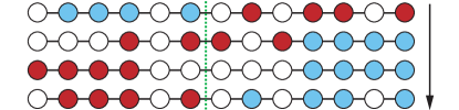
Figure 7: The initial (first row), goal (last row) and intermediate configurations of two groups of $4$ robots to be exchanged. Each group is marked with a different color/shade. The unshaded discs do not belong to either of the two group.

To do the grouping, we first apply a herding operation that moves one group of robots to one end of $P$. In Fig. 7, this is done to the group of lightly-shaded robots to move them to the right side (the second row of Fig. 7). Then, another herding operation is performed to move the other group to the other end of $P$ (the third row of Fig. 7). In the third and last step, two parallel ``reversed'' herding operations are carried out on two disjoint segments of $P$ to move them to their desired goal locations. This is best understood by viewing the process as applying the herding operation to the goal configuration. As an example, in Fig. 7, from the goal configuration (last row), we may readily apply two herding operations to move two groups of robots to the two ends of $P$ as shown in the third row of the figure. Because each herding operation takes $O(\ell)$ steps, the overall operation takes $O(\ell)$ steps as well. It is clear that in the end, a robot not in the two groups will not have any net movement on $P$ because the relative orders of these robots (unshaded ones in Fig. 7) never change.  ∎∎

Next, we generalize Lemma 7 to a tree embedded in a grid. On a tree graph $T$, we call a subgraph a path branch of $T$ if the subgraph is a path with no other attached branches. That is, all vertices of the subgraph have degrees one or two in $T$.

Theorem 8.

Let $T$ be a tree of diameter $d$ embedded in a grid. Let $P$ be a length $\ell$ path branch of $T$. Then, a group of robots on $P$ can be exchanged with robots on $T$ outside $P$ in $O(d)$ steps without net movement of other robots. The relocation may be performed using flip($\cdot$) on $T$.

Proof.

We temporarily limit the tree $T$ such that, after picking a proper main path that contains $P$ and deleting this main path, there are only paths left. That is, we assume all vertices with degree three or four are on a single path containing $P$. An example of such a tree $T$ and the exchange problem is given in the top row of Fig. 8. In the figure, the main path is the long horizontal path and $P$ is the path on the left of the dotted split line. We call other paths off the main path side branches. Once this version is proven, the general version readily follows because all possible tree structures are considered in this special example, i.e., there may be either one or two branches coming out of a node on the main branch. The rest of the paper will only use the less general version. For ease of reference, for the two groups of robots, we denote the group fully on $P$ as $g^{1}$ and the other group as $g^{2}$. In the example, $g^{1}$ has a light shade and $g^{2}$ has a darker shade.

\begin{overpic}[width=216.81pt,tics=5]{./figures/tree-move-2-eps-converted-to.pdf} \put(51.0,23.0){{\small$r^{2}_{1}$}} \put(51.0,36.0){{\small$r^{2}_{2}$}} \put(69.5,42.0){{\small$r^{2}_{3}$}} \put(76.3,42.0){{\small$r^{2}_{4}$}} \end{overpic}

Figure 8: The initial (first row) and three intermediate configurations in solving the problem of switching the location of these robots on a tree.

To start, we first solve part of the relocation problem on the main path, which can be done in $O(d)$ steps by Lemma 7. After the step, the robots involved in the first step are no longer relevant. In the example, this is to exchange the robots marked with small arrows in the first row of Fig. 8. After the relocation of these robots is completed, we remove their shades.

In the second step, the relevant robots in $g^{2}$ on the side branch are moved so that they are just off the main path. We also assign priorities to these robots based on their closeness to $P$ and break ties randomly. For a robot labeled $i$ in a group $g^{j}$, we denote the robot as $r_{i}^{j}$. For our example, this current step yields the third row of Fig. 8 with the priorities marked. Since the moves are done in parallel and each branch is of length at most $d$, only $O(d)$ steps are needed.

In the third step, robots from $g^{2}$ will move out of the side branches in the order given, one immediately after the other (when possible). For the example (third row of Fig. 8), $r_{1}^{2}$ will move first. $r_{2}^{2}$ will follow. Then $r_{3}^{2}$, followed by $r_{4}^{2}$. Using the same inductive argument from the proof of Lemma 6, we observe that all robots from $g^{2}$ on the side branch can be moved off the side branches (and reach their goals on the main path) in $O(d)$ time. As the relevant robots from $g^{1}$ also move across the split line, they will fill in side branches in opposite order to when the robots from $g_{2}$ are moved out of the branches. In the example, this means that the branch where $r_{3}^{2}$ and $r_{4}^{2}$ were on will be populated with robots from $g^{1}$ first, followed by the branch where $r_{2}^{2}$ was, and finally the branch where $r_{1}^{2}$ was. This ensures that at the end of this step, any robot not in $g^{1}$ and $g^{2}$ will have no net movement. The number of steps for this is again $O(d)$.

In the last step, we simply reverse the second step, which takes another $O(d)$ steps. Putting everything together, $O(d)$ steps are sufficient for completing the task.

Combining all steps, only $O(d)$ steps are required to complete the desired exchange. To see that the same conclusion holds for more general trees with side branches that are not simple paths, we simply need to do the second step and third step more carefully. But, because we are only moving at most $O(d)$ robots, using an amortization argument, it is straightforward to see that the $O(d)$ bound does not change.  ∎∎

We note that many of the operations used to prove Lemma 6, Lemma 7, and Theorem 8 can be combined without changing the outcome. However, doing so will make the proofs less modular. Given the focus of the current paper which is to construct a polynomial time algorithm with constant factor optimality guarantee, we opt for clarity instead of pursuing a smaller asymptotic constant.

IV-D Tree Forming and Robot Routing

We proceed to prove Theorem 4 by showing in detail how to carry out a single iteration of SaG, which boils down to partitioning the robot exchanges into robot exchanges on trees, to which Theorem 8 can then be applied. The proof itself can be subdivided into three steps:

• Splitting and initial tree forming, where a grid is partitioned into two roughly equal halves and trees are initial formed across the partition line for facilitating exchanging of two groups of robots.

• Tree post-processing, which addresses the issue where two initial trees might have ``$+$'' like crossovers.

• Final robot routing, which actually carries through the robot routing process and resolve some final issues.

Proof of Theorem 4.

Splitting and initial tree forming. In a split, we always split along the longer side of the current grid. Since $m_{\ell}\geq m_{s}$, the $m_{\ell}\times m_{s}$ grid is split into two grids of dimensions $\lceil m_{\ell}/2\rceil\times m_{s}$ and $\lfloor m_{\ell}/2\rfloor\times m_{s}$, respectively. For convenience, we denote the two split grids as $G_{1}$ and $G_{2}$, respectively. Recall that in the group operation, we want to exchange robots so that a robot with goal in $G_{1}$ (resp., $G_{2}$) resides in $G_{1}$ (resp., $G_{2}$) at the end of the operation. To do this efficiently, we need to maximize the parallelism. This is achieved through the computation of a set of $m_{s}$ trees with which we can apply Theorem 8. We will use the example from Fig. 9 to facilitate the higher level explanation.

\begin{overpic}[width=216.81pt,tics=10]{./figures/aggregate-tree-2-eps-converted-to.pdf} \put(-1.0,50.0){{\small$G_{2}$}} \put(-1.0,8.0){{\small$G_{1}$}} \put(23.0,-4.0){{\small(a)}} \put(72.5,-4.0){{\small(b)}} \end{overpic}

Figure 9: (a) A $9\times 7$ grid is split into two grids $G_{1}$ and $G_{2}$ of sizes $4\times 7$ and $5\times 7$, respectively. The dark-shaded robots' final goals are in $G_{2}$. (b) The grid is partitioned into (possibly non-disjoint) trees to allow the dark-shaded robots that are not already in $G_{2}$ to exchange with robots (lightly-shaded ones) that should be moved to $G_{1}$.

Assume that the grid is oriented so that $m_{s}$ is the number of columns and $m_{\ell}$ is the number of rows (see Fig. 9). The trees that will be built will be based on the columns of one of the split graphs, say $G_{2}$. A column $i$ of $G_{2}$ is a path of length $\lfloor m_{\ell}/2\rfloor-1$ with $\lfloor m_{\ell}/2\rfloor$ robots on it. Suppose $k_{i}$ of these robots have goals outside $G_{2}$ (the lightly-shaded ones in Fig. 9 (b)), then it is always possible to find $k_{i}$ robots (the dark-shaded ones in Fig. 9(b)) on $G_{1}$ that must go to $G_{2}$. A tree $T_{i}$ is built to allow the exchange of these $2k_{i}$ robots such that the part of $T_{i}$ in $G_{2}$ is simply column $i$. That is, the $m_{s}$ trees to be built do not overlap in $G_{2}$.

For a column $i$ in $G_{2}$ with $k_{i}$ robots to be moved to $G_{1}$, it is not always possible to find exactly $k_{i}$ robots on column $i$ of $G_{1}$. This makes the construction of the trees in $G_{1}$ more complex. The construction is done in two steps. In the first step, robots to be moved to $G_{2}$ are grouped in a distance optimal manner, which induces a preliminary tree structure. Focusing on $G_{1}$, we know the number of robots that must be moved across the split line in each column (see Fig. 10). For each robot to be moved across the split line, the distance between the robot and all the possible exits of $G_{1}$ is readily computed. Once these distances are computed, a standard matching procedure can be run to assign each robot an exit point that minimizes the total distance traveled by these robots [72, 48]. The assignment has a powerful property that we will use later. For each robot, either a straight or an $L$ shaped path can be obtained based on the assignment. Merging these paths for robots exiting from the same column then yields a tree for each column (see Fig. 9(b)). Note that each tree has a single vertical segment.

\begin{overpic}[width=216.81pt,tics=10]{./figures/assign-move-2-eps-converted-to.pdf} \put(28.4,38.0){{\small$2$}} \put(35.3,38.0){{\small$3$}} \put(42.0,38.0){{\small$2$}} \put(48.8,38.0){{\small$4$}} \put(55.6,38.0){{\small$0$}} \put(62.6,38.0){{\small$1$}} \put(69.2,38.0){{\small$3$}} \end{overpic}

Figure 10: For the example given in Fig. 9, this figure highlights $G_{1}$, the robots that must be moved to $G_{2}$, and how many robot need to be moved through the top of $G_{1}$ along each column. Regarding distance, the bottom left robot needs to travel $4$ edges to exit $G_{1}$ through the left most column. It needs to travel $4+7-1=10$ edges to exit from the right most column.

Tree post-processing. In the second step, the trees are post-processed to remove crossings between them. Example of such a crossing we refer to is illustrated in Fig. 11(a) (dotted lines). Formally, we say two trees $T_{1}$ and $T_{2}$ has a crossover if a horizontal path of $T_{1}$ intersects with a vertical path of $T_{2}$, with the additional requirement that one of the involved horizontal path from one tree forms a $+$ with the vertical segment of the other tree. For example, Fig. 11(b) is not considered a crossover.

\begin{overpic}[width=216.81pt,tics=10]{./figures/crossover-removal-2-eps-converted-to.pdf} \put(8.0,-4.0){{\small(a)}} \put(46.0,-4.0){{\small(b)}} \put(82.0,-4.0){{\small(c)}} \end{overpic}

Figure 11: (a) Example of a tree crossover (dotted paths) and its removal (solid paths) without increasing the total distance. Note that only the relevant paths of the two trees are shown. (b) An intersection that is not considered a crossover. (c) An impossible crossover scenario.

For each crossover, we update the two trees to remove the crossover, as illustrated in Fig. 11(a). The removal will not change the total distance traveled by the two (or more) affected robots but will change the path for these robots. To see that the process will end, note that one of the two involved paths is shortened. Since there are finite number of such paths and each path can only be shortened a finite number of times, the crossover removal process can get rid of all crossovers. We will show later this can be done in polynomial computation time when we perform algorithm analysis. We note here that the crossover scenario in Fig. 11(c) cannot happen because a removal would shorten the overall length, which contradicts the assumption that these paths have the shortest total distance.

Final robot routing. At the end of the crossover removal process, we may first route all robots on a tree branch that do not have overlaps with other trees. However, this does not route all robots because it is possible for the tree structures for different columns to overlap horizontally (see Fig. 12). For two trees that partially overlap with each other (e.g., the left and middle two trees in Fig. 12), one of the trees does not extend lower (row wise) than the row where the overlap occurs. Otherwise, this yields a crossover, which should have already been removed. For two overlapping trees $T_{1}$ and $T_{2}$, we say $T_{1}$ is a follower of $T_{2}$ if a robot going to $T_{2}$ must pass through the vertical path of $T_{1}$. In the example from Fig. 12, $T_{1}$ is a follower of $T_{2}$. Similarly, the right (green) tree is a follower of $T_{1}$.

\begin{overpic}[width=195.12767pt,tics=10]{./figures/artifact-2-eps-converted-to.pdf} \put(32.0,28.0){{\small$1$}} \put(39.0,28.0){{\small$2$}} \put(52.3,28.0){{\small$1$}} \put(25.0,18.0){{\small{\color[rgb]{0.4,0.1,0.6}$T_{2}$}}} \put(60.0,5.0){{\small{\color[rgb]{1,0,0}$T_{1}$}}} \end{overpic}

Figure 12: Illustration of overlaps between tree structures for different columns. For the four shaded robots to be moved, one must be moved through the left most vertical path, two must be moved through the middle vertical path, and the last must be moved through the right most vertical path.

We state some readily observable properties of overlapping trees: (i) two trees may have at most one overlapping horizontal branch (otherwise, there must be a path crossover), (ii) because of (i), any three trees cannot pair wise overlap at different rows, and (iii) there must be at least one tree that is not a follower, e.g., the left (purple) tree in Fig. 12. We call this tree a leader. From a leader tree, we can recursively collect its followers, and the followers of these followers, and so on so forth. We call such a collection an interacting bundle (e.g., Fig. 12).

With these properties in mind, the group operation in a SaG iteration is carried out as follows. Because robots to be moved from $G_{2}$ to $G_{1}$ are on straight vertical paths, there are no interactions among them between different trees. Therefore, we only need to consider interactions of robots on $G_{1}$. For trees that have no overlap with other trees, Theorem 8 directly applies to complete the robot exchange on these trees in $O(m_{\ell})$ steps because each tree has diameter at most $2m_{\ell}$. In parallel, we can also complete the movement of all robots that should go from $G_{1}$ to $G_{2}$ which are not residing on a horizontal tree branch that overlaps with other trees, also in $O(m_{\ell})$ steps. After these robots are exchanged, we can effectively forget about them.

After the previous step, we are left to deal with robots on overlapping horizontal tree branches that must be moved (e.g., the shaded robots in Fig. 12). It is clear that different interacting bundles do not have any interactions; we only need to focus on a single bundle. This is actually straightforward; we use the example from Fig. 13 to facilitate the proof explanation. The routing of robots in this case follows a greedy approach starting from the left most tree, i.e., we essentially try to ``flush'' the shaded robots in the left-up direction, which can always be realized in two phases, each of which using at most $O(m_{\ell})$ makespan.

\begin{overpic}[width=216.81pt,tics=5]{./figures/bundle-eps-converted-to.pdf} \put(9.7,82.0){{\small$3$}} \put(23.0,82.0){{\small$3$}} \put(36.0,82.0){{\small$2$}} \put(49.4,82.0){{\small$6$}} \put(69.2,82.0){{\small$1$}} \end{overpic}

Figure 13: An example interacting bundle in detail. The top row is the initial configuration of the robots on the overlapping horizontal tree branches to be moved through the vertical paths. The numbers on the top of the vertical paths mark how many robots should be moved through that path. For example, $3$ of the shaded robots must be routed through the left most vertical path. The middle row and the bottom rows mark how the exchanges can be completed in two steps or phases.

Observe that the problem can be solved for the leader tree (left most tree in Fig. 13). At the same time, for each successive follower tree, the movement of robots can be partially solved for these follower trees. The middle row of Fig. 13 shows how this can be done for each tree. Formally, if a horizontal branch is shared by two trees, say $T_{2}$ and its follower $T_{1}$, then we obtain a simple exchange problem of moving a few robots through a path on $T_{2}$. In the figure, these are the first and fourth trees from the left, with the dotted lines marking the path. If a horizontal branch is shared by three or more trees, we get an exchange problem on a tree. In the figure, the middle three trees create such a problem. For this, Theorem 8 applies with minor modifications. All the exchange problems can be carried out in parallel because there is no further interaction between them. It takes $O(m_{\ell})$ steps to complete, after which we are left with another set of exchange problems, each of which is on a path (e.g., the three problems in the last row of Fig. 13). Lemma 7 applies to yield $O(m_{\ell})$ required steps.

Stitching everything together, the first iteration of SaG on an $m_{\ell}\times m_{s}$ grid can be completed in $O(m_{\ell})$ steps. In the next iteration, we are working with grids of sizes $\lceil m_{\ell}/2\rceil\times m_{s}$, which requires $O(\max\{\lceil m_{\ell}/2\rceil,m_{s}\})$ steps. Following the simple recursion, which terminates after $O(\log m_{\ell})$ iterations, we readily obtain that $O(m_{\ell})$ steps are sufficient for solving the entire problem.  ∎∎

V Complexity and Solution Optimality Properties of the SaG Algorithm

In this section, we establish two key properties of SaG, namely, its polynomial running-time and asymptotic solution optimality.

V-A Time Complexity of SaG

The SaG algorithm is outlined in Algorithm 1, which summarizes the results from Section IV in the form of an algorithm. At Lines 1-1, a partition of the current grid $G$ is made, over which initial path planning is performed to generate the trees for grouping the robots into the proper subgraph. Then, at Line 1, crossovers are resolved. At Line 1, the final paths are scheduled, from which the robot moves can be extracted. This step also yields where each robot will end up at in the end of the iteration, which becomes the initial configuration for the next iteration (if there is one). After the main iteration steps are complete, at Lines 1-1, the algorithm recursively calls itself on smaller problem instances. The special case here is when the problem is small enough (Line 1), in which case the problem is directly solved without further splitting.

Input : $G=(V,E)$: an $m_{\ell}\times m_{s}$ grid graph

$X_{I}$: initial robot configurations

$X_{G}$: goal robot configurations

Output : $M=\langle M_{1},M_{2},\ldots\rangle$: a sequence of moves

1

2

%Run matching and construct initial trees

3 $(G_{1},G_{2})\leftarrow\textsc{Split}(G)$

4 $\mathcal{P}\leftarrow\textsc{MatchAndPlanPath}(G,X_{I},X_{G})$

%Remove crossovers

5 $\mathcal{P}^{\prime}\leftarrow\textsc{ResolveCrossovers}(\mathcal{P})$

%Schedule the sequence of moves

6 $(M,X_{I}^{\prime})\leftarrow\textsc{ScheduleMoves}(\mathcal{P}^{\prime})$

%Recursively solve smaller sub-problems

7 foreach $G_{i},i=1,2$ do

8       if $row(G_{i})\leq 3$ and $col(G_{i})\leq 3$ then

9            $M=M+\textsc{Solve}(G_{i},X_{I}^{\prime}|_{G_{i}},X_{G}|_{G_{i}})$

10       else

11            $M=M+\textsc{SaG}(G_{i},X_{I}^{\prime}|_{G_{i}},X_{G}|_{G_{i}})$

12       end if

13      

14 end foreach

15

16

return $M$

Algorithm 1 SplitAndGroup ($G$, $X_{I}$, $x_{G}$)

We now proceed to bound the running time of SaG. It is straightforward to see that the Split routine takes $O(|V|)=O(m_{\ell}m_{s})$ running time. MatchAndPlanPath can be implemented using the standard Hungarian algorithm [72], which runs in $O(|V|^{3})$ time.

For ResolveCrossovers, we may implement it by starting with an arbitrary robot that needs to be moved across the split line and check whether the path it is on has crossovers that need to be resolved. Checking one path with another can be done in constant time because each path has only two straight segments. Detecting a crossover then takes up to $O(|V|)$ running time. We note that, as a crossover is resolved, one of the two paths will end up being shorter (see, e.g., Fig. 11). We then repeat the process with this shorter path until no more crossover exists. Naively, because the path keeps getting shorter, this process will end in at most $O(|V|)$ steps. Therefore, all together, ResolveCrossovers can be completed in $O(|V|^{3})$ time.

The ScheduleMoves routine simply extracts information from the already planned path set $\mathcal{P}^{\prime}$ and can be completed in $O(|V|)$ running time. The Solve routine takes constant time.

Adding everything up, an iteration of SaG can be carried out in $O(|V|^{3})$ time using a naive implementation. Summing over all iterations, the total running time is

$$O(|V|^{3})+2O((\frac{|V|}{2})^{3})+4O((\frac{|V|}{4})^{3})+\ldots=O(|V|^{3}),$$

which is low-polynomial with respect to the input size.

V-B Optimality Guarantees

Having established that SaG is a polynomial time algorithm that solves MPP with sub-linear makespan, we now show that SaG is an $O(1)$-approximate makespan optimal algorithm for MPP in the average case. Moreover, SaG also computes a constant factor distance optimal solution in a weaker sense. To establish these, we first show that for fixed $m_{\ell}m_{s}$ that is large, the number of MPP instances with $o(m_{\ell}+m_{s})$ makespan is negligible.

Lemma 9.

The fraction of MPP instances on a fixed graph $G$ as an $m_{\ell}\times m_{s}$ grid with $o(m_{\ell}+m_{s})$ makespan is no more than $(\frac{1}{2})^{\frac{m_{\ell}}{4}}$ for sufficiently large $m_{\ell}m_{s}$.

Proof.

Let $(G,X_{I},X_{G})$ be an MPP instance wth $G$ being a $m_{\ell}\times m_{s}$ grid. Without loss of generality, we may assume that $X_{I}$ is arbitrary and $X_{G}$ is a row-major ordering of the robots, i.e., with the $i$-th row containing the robots labeled $(i-1)m_{\ell}+1,(i-1)m_{\ell}+2,\ldots,im_{\ell}$, in that order. Then, over all possible instances, $\frac{1}{4}$ of instances have $X_{I}$ with robot $1$ having a distance of $\frac{1}{4}(m_{\ell}+m_{s})$ or less from robot $1$'s location in $X_{G}$ (note that the number is $\frac{1}{4}$ instead of $\frac{1}{16}$ because $m_{s}$ maybe as small as 2). Let these $\frac{1}{4}$ instances be $\mathcal{P}_{1}$. Among $\mathcal{P}_{1}$, again about $\frac{1}{4}$ of instances have have $X_{I}$ with robot $2$ having a distances of $\frac{1}{4}(m_{\ell}+m_{s})$ or less from robot $2$'s location in $X_{G}$. Following this reasoning and limiting to the first $\frac{m_{\ell}}{4}$ robots, we may conclude that the fraction of instances with $o(m_{\ell}+m_{s})$ makespan is no more than $(\frac{1}{2})^{\frac{m_{\ell}}{4}}$ for sufficiently large $m_{\ell}m_{s}$.  ∎∎

Lemma 9 is conservative but sufficient for establishing that SaG delivers an average case $O(1)$-approximation for makespan. That is, since only an exponentially small number of instances have small makespan, the average makespan ratio is clearly constant, that is,

Theorem 10.

On average and in polynomial time, SaG computes $O(1)$-approximate makespan optimal solutions for MPP.

Proof.

For a fixed $G$ as an $m_{\ell}\times m_{s}$ grid, Lemma 9 says that no more than a $(\frac{1}{2})^{\frac{m_{\ell}}{4}}$ fraction of instances have sub-linear makespan (the minimum possible makespan is $1$). For the rest of the instances, their makespan is linear, i.e., $\Omega(m_{\ell}+m_{s})$. On the other hand, Algorithm 1 guarantees a makespan of $O(m_{\ell}+m_{s})$. We may then compute the expected (i.e., average) makespan ratio over all instances of MPP for the same $G$ as no more than (for sufficiently large $m_{\ell}$)

$$(\frac{1}{2})^{\frac{m_{\ell}}{4}}\frac{O(m_{\ell}+m_{s})}{1}+(1-(\frac{1}{2})^{\frac{m_{\ell}}{4}})\frac{O(m_{\ell}+m_{s})}{\Omega(m_{\ell}+m_{s})}=O(1).$$

This establishes the claim of the theorem.  ∎∎

SaG can also provide guarantees on total distance optimality. In this case, because every robot contributes to the total distance, a weaker guarantee is ensured (in the case of makespan, one robot's makespan dominates the makespan of all other robots). This leads us to work with a typical (i.e., average) MPP instance instead of working with averages of makespan optimality ratio over all instances. That is, for the makespan case, we first compute the optimality ratio for each instance, which is subsequently averaged. For total distance, we work with a typical random instance and compute the optimality ratio for such a typical instance.

Theorem 11.

For an average MPP instance, SaG computes an $O(1)$-approximate total distance optimal solution.

Proof.

For an average MPP instance, each robot incurs a minimum travel distance of $\Omega(m_{\ell})$; therefore, the minimum total distance for all robots, in expectation, is $\Omega(m_{s}m_{\ell}^{2})$ because there are $m_{s}m_{\ell}$ robots. On the other hand, because SaG produces a solution with an $O(m_{\ell})$ makespan, each robot travels a distance of $O(m_{\ell})$. Summing this over all robots, the solution from SaG has a total distance of $O(m_{s}m_{\ell}^{2})$. This matches the lower bound $\Omega(m_{s}m_{\ell}^{2})$ .  ∎∎

VI Extensions

In this section, we show that SaG readily generalizes to environments other than 2D rectangular grids, including high dimensional grids and continuous environments.

VI-A High Dimensions

SaG can be extended to work for grids of arbitrary dimensions. For dimensions $d\geq 2$, let the grid be $m_{1}\times\ldots\times m_{d}$. Two updates to SaG are needed to make it work for higher dimensions. First, the split line should be updated to a split plane of dimension $d-1$. In the case of $d=2$, two iterations will halve all dimensions. In the case of general $d$, $d$ iterations are required. Thus, the approach produces a makespan of $O(d(m_{1}+\ldots m_{d}))$ where $m_{i}$ is the side length of $i$-th dimension. Second, the crossover check becomes more complex; each check now takes $O(d)$ time instead of $O(1)$ time because each path, though still having up to two straight pieces, requires $O(d)$ coordinates to describe. Other than these changes, the rest of SaG continues to work with some minor modifications to the scheduling procedure (which can again be proven to be correct using inductive proofs). The updated SaG algorithm for dimension $d$ therefore runs in $O(d^{2}|V|^{3})$ time because $d$ iterations of split and group are need to halve all dimensions and each iteration takes $O(d|V|^{3})$ time. The optimality guarantees, e.g., Theorems 10 and 11, also carry over.

VI-B Well-Connected Environments

The selection of $G$ as a grid plays a critical role in proving the desirable properties of SaG. In particular, two features of grid graphs are used. First, grids are composed of small cycles, which allow the 2-switch operation to be carried out locally. This in turn allows multiple 2-switch operations to be carried out in parallel. Second, restricting to two adjacent rows (or columns) of a rectangular grid (e.g., row 4 and row 5 in Fig. 9(a)), multiple 2-switches can be completed between these two rows in a constant number of steps. As long as the environment possesses these two features, SaG works. We call such environments well-connected.

More precisely, a well-connected environment, $\mathcal{E}$, is one with the following properties. Let $G$ be an $m_{\ell}\times m_{s}$ rectangular grid that contains $\mathcal{E}$. Unlike earlier grids, here, $G$ is not required to have unit edge lengths; a cell of $G$ is only required to be of rectangular shape with $O(1)$ side lengths. Let $r_{1}$ and $r_{2}$ be two arbitrary adjacent rows of $G$, and let $c_{1}\in r_{1}$, $c_{2}\in r_{2}$ be two neighboring cells (see, e.g., Fig. 14). The only requirement over $\mathcal{E}$ is that a robot in $c_{1}$ and a robot in $c_{2}$ may exchange residing cells locally, without affecting the configuration of other robots. In terms of the example in Fig. 14, the two shaded robots (other robots are not drawn) must be able to exchange locations in constant makespan within a region of constant radius. The requirement then implies that parallel exchanges of robots between $r_{1}$ and $r_{2}$ can be performed with a constant makespan. The same requirement applies to two adjacent columns of $G$.

\begin{overpic}[width=173.44534pt,tics=10]{./figures/grid-like-eps-converted-to.pdf} \put(105.0,55.0){{\small{\color[rgb]{1,.5,0}$G$}}} \put(7.0,42.0){{\small$\mathcal{E}$}} \put(105.0,40.0){{\small{\color[rgb]{1,.5,0}$r_{1}$}}} \put(105.0,25.0){{\small{\color[rgb]{1,.5,0}$r_{2}$}}} \put(77.0,19.0){{\small{\color[rgb]{1,0,0}$c_{1}$}}} \put(77.0,36.0){{\small{\color[rgb]{1,0,0}$c_{2}$}}} \end{overpic}

Figure 14: Illustration of a well-connected non-grid graph.

Subsequently, given an arbitrary well-connected environment $\mathcal{E}$ and an initial robot configuration $X_{I}$, the steps from SaG can be readily applied to reach an arbitrary $X_{G}$ that is a permutation of $X_{I}$. As long as pairwise robot exchanges can be computed efficiently, the overall generalized SaG algorithm also runs efficiently while maintaining the optimality guarantees. We note that the definition of well-connectedness can be further generalized to certain continuous settings. Fig. 15 provides a discrete example and a continuous example of well-connected settings, which include both the environment and the robots.

\begin{overpic}[width=195.12767pt,tics=10]{./figures/honeycomb-eps-converted-to.pdf} \end{overpic}

Figure 15: Examples of well-connected settings, with both environments and robots.

As mentioned in Sec. I, well-connected environments are frequently found in real-world applications, e.g., automated warehouses at Amazon and road networks in cities like Manhattan. Our theoretical results imply that such environments are in fact quite optimal in their design in terms of being able to efficiently route robots.

VII Conclusion and Future Work

In this work, we developed a low-polynomial time algorithm, SaG, for solving the multi-robot path planning problem in grids and grid-like, well-connected environments. The solution produced by SaG is within a constant factor of the best possible makespan on average. In a weaker sense, SaG also provide a constant factor approximation on total distance optimality. SaG applies to problems with the maximum possible density in graph-based settings and supports certain continuous problems as well.

The development of SaG opens up many possibilities for promising future work. On the theoretical side, SaG gets us closer to the goal of a finding a PTAS (polynomial time approximation scheme) for optimal multi-robot path planning. Also, it would be desirable to remove the probabilistic element (i.e., the ``in expectation'' part) from the guarantees. On the practical side, noting that we have only looked at the case with the highest robot density, it is promising to exploit the combination of global decoupling and network flow techniques to seek more optimal algorithms for cases with lower robot density.

References

- [1] O. Goldreich, ``Finding the shortest move-sequence in the graph-generalized 15-puzzle is np-hard,'' in Studies in Complexity and Cryptography. Miscellanea on the Interplay between Randomness and Computation. Springer, 2011, pp. 1–5.
- [2] J. Yu, ``Intractability of optimal multi-robot path planning on planar graphs,'' IEEE Robotics and Automation Letters, vol. 1, no. 1, pp. 33–40, 2016.
- [3] J. Banfi, N. Basilico, and F. Amigoni, ``Intractability of time-optimal multirobot path planning on 2d grid graphs with holes,'' IEEE Robotics and Automation Letters, vol. 2, no. 4, pp. 1941–1947, 2017.
- [4] S. D. Han, E. J. Rodriguez, and J. Yu, ``Sear: A polynomial-time expected constant-factor optimal algorithmic framework for multi-robot path planning,'' in Proceedings IEEE/RSJ International Conference on Intelligent Robots & Systems, 2018.
- [5] J. Yu, ``Expected constant-factor optimal multi-robot path planning in well-connected environments,'' in Multi-Robot and Multi-Agent Systems (MRS), 2017 International Symposium on. IEEE, 2017, pp. 48–55.
- [6] M. A. Erdmann and T. Lozano-Pérez, ``On multiple moving objects,'' in Proceedings IEEE International Conference on Robotics & Automation, 1986, pp. 1419–1424.
- [7] S. M. LaValle and S. A. Hutchinson, ``Optimal motion planning for multiple robots having independent goals,'' IEEE Transactions on Robotics & Automation, vol. 14, no. 6, pp. 912–925, Dec. 1998.
- [8] Y. Guo and L. E. Parker, ``A distributed and optimal motion planning approach for multiple mobile robots,'' in Proceedings IEEE International Conference on Robotics & Automation, 2002, pp. 2612–2619.
- [9] D. Silver, ``Cooperative pathfinding,'' in The 1st Conference on Artificial Intelligence and Interactive Digital Entertainment, 2005, pp. 23–28.
- [10] M. R. K. Ryan, ``Exploiting subgraph structure in multi-robot path planning,'' Journal of Artificial Intelligence Research, vol. 31, pp. 497–542, 2008.
- [11] R. Jansen and N. Sturtevant, ``A new approach to cooperative pathfinding,'' in In International Conference on Autonomous Agents and Multiagent Systems, 2008, pp. 1401–1404.
- [12] R. Luna and K. E. Bekris, ``Push and swap: Fast cooperative path-finding with completeness guarantees,'' in Proceedings International Joint Conference on Artificial Intelligence, 2011, pp. 294–300.
- [13] T. Standley and R. Korf, ``Complete algorithms for cooperative pathfinding problems,'' in Proceedings International Joint Conference on Artificial Intelligence, 2011, pp. 668–673.
- [14] J. van den Berg, J. Snoeyink, M. Lin, and D. Manocha, ``Centralized path planning for multiple robots: Optimal decoupling into sequential plans,'' in Robotics: Science and Systems, 2009.
- [15] K. Solovey and D. Halperin, ``-color multi-robot motion planning,'' in Proceedings Workshop on Algorithmic Foundations of Robotics, 2012.
- [16] J. Yu and S. M. LaValle, ``Multi-agent path planning and network flow,'' in Algorithmic Foundations of Robotics X, Springer Tracts in Advanced Robotics. Springer Berlin/Heidelberg, 2013, vol. 86, pp. 157–173.
- [17] M. Turpin, K. Mohta, N. Michael, and V. Kumar, ``CAPT: Concurrent assignment and planning of trajectories for multiple robots,'' International Journal of Robotics Research, vol. 33, no. 1, pp. 98–112, 2014.
- [18] H. Choset, K. M. Lynch, S. Hutchinson, G. Kantor, W. Burgard, L. E. Kavraki, and S. Thrun, Principles of Robot Motion: Theory, Algorithms, and Implementations. Cambridge, MA: MIT Press, 2005.
- [19] J. van den Berg, M. C. Lin, and D. Manocha, ``Reciprocal velocity obstacles for real-time multi-agent navigation,'' in Proceedings IEEE International Conference on Robotics & Automation, 2008, pp. 1928–1935.
- [20] M. S. Branicky, M. M. Curtiss, J. Levine, and S. Morgan, ``Sampling-based planning, control and verification of hybrid systems,'' IEE Proceedings Control Theory and Applications, vol. 153, no. 5, p. 575, 2006.
- [21] O. Khatib, ``Real-time obstacle avoidance for manipulators and mobile robots,'' The international journal of robotics research, vol. 5, no. 1, pp. 90–98, 1986.
- [22] M. G. Earl and R. D'Andrea, ``Iterative milp methods for vehicle-control problems,'' IEEE Transactions on Robotics, vol. 21, no. 6, pp. 1158–1167, 2005.
- [23] K. E. Bekris, K. I. Tsianos, and L. E. Kavraki, ``A decentralized planner that guarantees the safety of communicating vehicles with complex dynamics that replan online,'' in 2007 IEEE/RSJ International Conference on Intelligent Robots and Systems. IEEE, 2007, pp. 3784–3790.
- [24] R. A. Knepper and D. Rus, ``Pedestrian-inspired sampling-based multi-robot collision avoidance,'' in 2012 IEEE RO-MAN: The 21st IEEE International Symposium on Robot and Human Interactive Communication. IEEE, 2012, pp. 94–100.
- [25] J. Alonso-Mora, R. Knepper, R. Siegwart, and D. Rus, ``Local motion planning for collaborative multi-robot manipulation of deformable objects,'' in 2015 IEEE International Conference on Robotics and Automation (ICRA). IEEE, 2015, pp. 5495–5502.
- [26] D. Halperin, J.-C. Latombe, and R. Wilson, ``A general framework for assembly planning: The motion space approach,'' Algorithmica, vol. 26, no. 3-4, pp. 577–601, 2000.
- [27] B. Nnaji, Theory of Automatic Robot Assembly and Programming. Chapman & Hall, 1992.
- [28] S. Rodriguez and N. M. Amato, ``Behavior-based evacuation planning,'' in Proceedings IEEE International Conference on Robotics & Automation, 2010, pp. 350–355.
- [29] T. Balch and R. C. Arkin, ``Behavior-based formation control for multirobot teams,'' IEEE Transactions on Robotics & Automation, vol. 14, no. 6, pp. 926–939, 1998.
- [30] S. Poduri and G. S. Sukhatme, ``Constrained coverage for mobile sensor networks,'' in Proceedings IEEE International Conference on Robotics & Automation, 2004.
- [31] B. Shucker, T. Murphey, and J. K. Bennett, ``Switching rules for decentralized control with simple control laws,'' in American Control Conference, Jul 2007, pp. 1485–1492.
- [32] B. Smith, M. Egerstedt, and A. Howard, ``Automatic generation of persistent formations for multi-agent networks under range constraints,'' ACM/Springer Mobile Networks and Applications Journal, vol. 14, no. 3, pp. 322–335, June 2009.
- [33] H. Tanner, G. Pappas, and V. Kumar, ``Leader-to-formation stability,'' IEEE Transactions on Robotics & Automation, vol. 20, no. 3, pp. 443–455, Jun 2004.
- [34] D. Fox, W. Burgard, H. Kruppa, and S. Thrun, ``A probabilistic approach to collaborative multi-robot localization,'' Autonomous Robots, vol. 8, no. 3, pp. 325–344, June 2000.
- [35] E. J. Griffith and S. Akella, ``Coordinating multiple droplets in planar array digital microfluidic systems,'' International Journal of Robotics Research, vol. 24, no. 11, pp. 933–949, 2005.
- [36] M. J. Matarić, M. Nilsson, and K. T. Simsarian, ``Cooperative multi-robot box pushing,'' in Proceedings IEEE/RSJ International Conference on Intelligent Robots & Systems, 1995, pp. 556–561.
- [37] D. Rus, B. Donald, and J. Jennings, ``Moving furniture with teams of autonomous robots,'' in Proceedings IEEE/RSJ International Conference on Intelligent Robots & Systems, 1995, pp. 235–242.
- [38] J. S. Jennings, G. Whelan, and W. F. Evans, ``Cooperative search and rescue with a team of mobile robots,'' in Proceedings IEEE International Conference on Robotics & Automation, 1997.
- [39] J. H. Reif, ``Complexity of the generalized mover's problem.'' DTIC Document, Tech. Rep., 1985.
- [40] J. F. Canny, The Complexity of Robot Motion Planning. Cambridge, MA: MIT Press, 1988.
- [41] P. Spirakis and C. K. Yap, ``Strong NP-hardness of moving many discs,'' Information Processing Letters, vol. 19, no. 1, pp. 55–59, 1984.
- [42] J. E. Hopcroft, J. T. Schwartz, and M. Sharir, ``On the complexity of motion planning for multiple independent objects; PSPACE-hardness of the ``warehouseman's problem'','' The International Journal of Robotics Research, vol. 3, no. 4, pp. 76–88, 1984.
- [43] S. Kloder and S. Hutchinson, ``Path planning for permutation-invariant multirobot formations,'' IEEE Transactions on Robotics, vol. 22, no. 4, pp. 650–665, 2006.
- [44] R. A. Hearn and E. D. Demaine, ``PSPACE-completeness of sliding-block puzzles and other problems through the nondeterministic constraint logic model of computation,'' Theoretical Computer Science, vol. 343, no. 1, pp. 72–96, 2005.
- [45] K. Solovey and D. Halperin, ``On the hardness of unlabeled multi-robot motion planning,'' in Robotics: Science and Systems (RSS), 2015.
- [46] M. Katsev, J. Yu, and S. M. LaValle, ``Efficient formation path planning on large graphs,'' in Proceedings IEEE International Conference on Robotics & Automation, 2013, pp. 3606–3611.
- [47] A. Adler, M. De Berg, D. Halperin, and K. Solovey, ``Efficient multi-robot motion planning for unlabeled discs in simple polygons,'' in Algorithmic Foundations of Robotics XI. Springer, 2015, pp. 1–17.
- [48] K. Solovey, J. Yu, O. Zamir, and D. Halperin, ``Motion planning for unlabeled discs with optimality guarantees,'' in Robotics: Science and Systems, 2015.
- [49] V. Auletta, A. Monti, M. Parente, and P. Persiano, ``A linear-time algorithm for the feasbility of pebble motion on trees,'' Algorithmica, vol. 23, pp. 223–245, 1999.
- [50] G. Goraly and R. Hassin, ``Multi-color pebble motion on graph,'' Algorithmica, vol. 58, pp. 610–636, 2010.
- [51] J. Yu, ``A linear time algorithm for the feasibility of pebble motion on graphs,'' arXiv:1301.2342, 2013.
- [52] J. Yu and D. Rus, ``Pebble motion on graphs with rotations: Efficient feasibility tests and planning,'' in Algorithmic Foundations of Robotics XI, Springer Tracts in Advanced Robotics, vol. 107. Springer Berlin/Heidelberg, 2015, pp. 729–746.
- [53] D. Ratner and M. Warmuth, ``The -puzzle and related relocation problems,'' Journal of Symbolic Computation, vol. 10, pp. 111–137, 1990.
- [54] J. Yu and S. M. LaValle, ``Structure and intractability of optimal multi-robot path planning on graphs,'' in Proceedings AAAI National Conference on Artificial Intelligence, 2013, pp. 1444–1449.
- [55] R. Alami, F. Robert, F. Ingrand, and S. Suzuki, ``Multi-robot cooperation through incremental plan-merging,'' in Robotics and Automation, 1995. Proceedings., 1995 IEEE International Conference on, vol. 3. IEEE, 1995, pp. 2573–2579.
- [56] S. Qutub, R. Alami, and F. Ingrand, ``How to solve deadlock situations within the plan-merging paradigm for multi-robot cooperation,'' in Intelligent Robots and Systems, 1997. IROS'97., Proceedings of the 1997 IEEE/RSJ International Conference on, vol. 3. IEEE, 1997, pp. 1610–1615.
- [57] M. Saha and P. Isto, ``Multi-robot motion planning by incremental coordination,'' in 2006 IEEE/RSJ International Conference on Intelligent Robots and Systems. IEEE, 2006, pp. 5960–5963.
- [58] G. Wagner and H. Choset, ``M*: A complete multirobot path planning algorithm with performance bounds,'' in Proceedings IEEE/RSJ International Conference on Intelligent Robots & Systems, 2011, pp. 3260–3267.
- [59] C. Ferner, G. Wagner, and H. Choset, ``Odrm* optimal multirobot path planning in low dimensional search spaces,'' in Robotics and Automation (ICRA), 2013 IEEE International Conference on. IEEE, 2013, pp. 3854–3859.
- [60] G. Sharon, R. Stern, A. Felner, and N. Sturtevant, ``Conflict-Based Search for Optimal Multi-Agent Path Finding,'' in Proc of the Twenty-Sixth AAAI Conference on Artificial Intelligence, 2012.
- [61] G. Sharon, R. Stern, M. Goldenberg, and A. Felner, ``The increasing cost tree search for optimal multi-agent pathfinding,'' Artificial Intelligence, vol. 195, pp. 470–495, 2013.
- [62] E. Boyarski, A. Felner, R. Stern, G. Sharon, O. Betzalel, D. Tolpin, and E. Shimony, ``Icbs: The improved conflict-based search algorithm for multi-agent pathfinding,'' in Eighth Annual Symposium on Combinatorial Search, 2015.
- [63] L. Cohen, T. Uras, T. Kumar, H. Xu, N. Ayanian, and S. Koenig, ``Improved bounded-suboptimal multi-agent path finding solvers,'' in International Joint Conference on Artificial Intelligence, 2016.
- [64] W. Hönig, T. S. Kumar, L. Cohen, H. Ma, H. Xu, N. Ayanian, and S. Koenig, ``Multi-agent path finding with kinematic constraints.'' in ICAPS, 2016, pp. 477–485.
- [65] P. Surynek, ``Towards optimal cooperative path planning in hard setups through satisfiability solving,'' in Proceedings 12th Pacific Rim International Conference on Artificial Intelligence, 2012.
- [66] E. Erdem, D. G. Kisa, U. Öztok, and P. Schueller, ``A general formal framework for pathfinding problems with multiple agents.'' in AAAI, 2013.
- [67] J. Yu and S. M. LaValle, ``Optimal multi-robot path planning on graphs: Complete algorithms and effective heuristics,'' IEEE Transactions on Robotics, vol. 32, no. 5, pp. 1163–1177, 2016.
- [68] H. Ma, J. Li, T. Kumar, and S. Koenig, ``Lifelong multi-agent path finding for online pickup and delivery tasks,'' in Proceedings of the 16th Conference on Autonomous Agents and MultiAgent Systems. International Foundation for Autonomous Agents and Multiagent Systems, 2017, pp. 837–845.
- [69] D. Atzmon, R. Stern, A. Felner, G. Wagner, R. Barták, and N.-F. Zhou, ``Robust multi-agent path finding,'' in Proceedings of the 17th International Conference on Autonomous Agents and MultiAgent Systems. International Foundation for Autonomous Agents and Multiagent Systems, 2018, pp. 1862–1864.
- [70] D. M. Kornhauser, ``Coordinating pebble motion on graphs, the diameter of permutation groups, and applications,'' Ph.D. dissertation, Massachusetts Institute of Technology, 1984.
- [71] B. Bollobás, Modern graph theory. Springer Science & Business Media, 2013, vol. 184.
- [72] H. W. Kuhn, ``The Hungarian method for the assignment problem,'' Naval Research Logistics Quarterly, vol. 2, pp. 83–97, 1955.