Near-Perfect Conversion of a Propagating Plane Wave into a Surface Wave Using Metasurfaces

Abstract

In this paper, theoretical and numerical studies of perfect/nearly-perfect conversion of a plane wave into a surface wave are presented. The problem of determining the electromagnetic properties of an inhomogeneous lossless boundary which would fully transform an incident plane wave into a surface wave propagating along the boundary is considered. An approximate field solution which produces a slowly growing surface wave and satisfies the energy conservation law is discussed and numerically demonstrated. The results of the study are of great importance for the future development of such devices as perfect leaky-wave antennas and can potentially lead to many novel applications.

I Introduction

Traditional leaky-wave antennas Oliner and Jackson (2007) at microwave frequencies are devices that convert between space and guided wave propagation modes. By introducing either periodic or continuous perturbation to a waveguide or transmission-line structure, portion of the guided power is designed to leak in a desired radiation direction. For a standard leaky-wave structure, the complex propagation constant describes the rate of exponential amplitude decay and the phase velocity along the guided wave direction. The characteristics of the radiated wave can be obtained from the field distribution over the radiating aperture. A comprehensive review on leaky-wave theory and techniques is available in Monticone and Alù (2015).

Since the aperture field distribution of a standard leaky-wave structure is different from a uniform-amplitude and linear-phase one, the conversion between the space and guided waves is not perfect. In the transmitting case, this translates to radiation into unwanted directions; in the receiving case, it means that the incoming plane wave from the scan direction is partially reflected and scattered, rather than completely transformed into the guided-mode wave. Recently, synthesis of a desired leaky-wave radiation characteristics associated with a custom aperture field distribution is receiving an increased interest using spatially varying perturbation structures—the waveguide width and the metallic post interval in a substrate-integrated waveguide Martinez-Ros et al. (2012); tensor sheet admittances in stacked metasurfaces on a ground plane Tierny and Grbic (2015); and the shape, size, and periodicity of locally anisotropic unit cell in the form of printed conductor patches on a grounded dielectric substrate Minatti et al. (2016a, b).

The problem of conversion of a propagating plane wave into a surface wave appears to be similar to that of anomalous reflection or refraction in underlying physics, where a propagating plane wave is converted into another propagating plane wave. Recently, it was recognized that manipulation of propagating waves using such devices as conventional reflectarrays and transmitarrays is accompanied by fundamental imperfections, associated with inevitable power scattered into undesired directions. Studies of non-local metasurfaces have demonstrated the possibility to create devices, which can perfectly transform a plane wave incident along one direction into a plane wave propagating into another direction Asadchy et al. (2016); Estakhri and Alù (2016). Now, both theoretical designs employing penetrable and impenetrable metasurfaces Epstein and Eleftheriades (2016); Kwon and Tretyakov (2017) and a practical realization based on the leaky-wave principle on a super-cell level Díaz-Rubio et al. (2017) are available. However, in sharp contrast to anomalous reflection, perfect conversion between space waves and guided waves is still elusive. No designs are available for the canonical transformation problem between a plane wave and a surface wave that promise perfect conversion devoid of spurious scattering in the limit of lossless constituents.

In Sun et al. (2012), the authors reported a periodic metasurface with linear reflection phase approximation based on the generalized law of reflection Yu et al. (2011) (similarly to conventional gratings), in which a power conversion efficiency of nearly a 100% was claimed. However, the reported structure cannot operate without introducing losses for an infinitely long structure, because otherwise a momentum mismatch between a propagating wave and a surface wave appears, not being able to excite a surface wave (full reflection of the propagating wave back into the free space). Furthermore, such a structure does not support a surface wave to propagate along the surface as the surface wave is not an eigensolution of the metasurface. As a result, the reported gradient metasurface, as an infinitely long converter, operates as a good absorber at steady state. For finite-length converters, the power conversion efficiency between a plane wave and a surface wave was theoretically and numerically studied in Qu et al. (2013). For periodic supercell-based gradient metasurface implementations, the decoupling effect taking place at the interface between supercells has a significant impact on efficiency. For a converter comprising two supercells, a high conversion efficiency of 78% was predicted.

Further, the authors also developed a surface plasmon polaritons (SPP) approach Sun et al. (2016) based on the generalized law of reflection Yu et al. (2011). The model consists of a meta-coupler, which is impedance matched to the free space and plasmonic metal sheet located below. Such a system allows creation of an SPP wave without decoupling effect. The authors claim to have a numerically predicted conversion efficiency of $94\%$. The design consists of two surfaces with an approximately half-wavelength separation between them. A single, low-profile design would have been more desirable. Furthermore, an SPP generated by a meta-coupler upon plane-wave illumination will go through additional refraction by the same meta-coupler with the wavenumber along the surface shifted further into the invisible range. This effect of higher-order spatial harmonics generation deep in the invisible range has not been investigated.

In Estakhri and Alù (2016), transformation of a propagating wave into a surface wave using metasurface was described, which is designed as a passive and lossy periodic structure. However, the reported conversion efficiency of such a metasurface is quite low ($\approx 7\%$). A transparent metasurface for transforming a beam wave into a surface wave and back into a beam wave was reported in Achouri and Caloz (2016a, b). Contrary to the claims, the propagating beam launched by the metasurface appears to be generated by active (i.e., source) metasurface constituents rather than being converted from the surface wave propagating along the metasurface.

In this paper, we theoretically and numerically investigate conversion of propagating plane waves to surface waves. In particular, we explain that it is not possible to create a point-wise lossless metasurface which would perfectly convert an incident plane wave into a single surface-wave mode carrying linearly growing power along the propagation direction (as required by the energy conservation). On the other hand, we present an approximate solution for the surface impedance of a metasurface which performs such a conversion with a high (predicted to be nearly 100%) efficiency. As an example, near-perfect conversion of a plane wave into a surface wave with a slow exponential growth is numerically tested. Such a solution is a special case of separable solutions to the Helmholtz equation, which consist of a single spatial harmonic. Although in this case the power growth law is different from the ideal linear dependence, we show that a very accurate approximate solution can be found if the exponential growth of a surface-bound eigenwave is slow enough. The appropriate surface impedance that realizes the envisioned conversion is found from the boundary condition using the total field distribution. Example designs are numerically tested to demonstrate near-perfect propagating wave-to-surface wave conversion performance. Furthermore, we show that non-local metasurfaces can emulate the active-lossy behaviour necessary for ideal conversion, without the need to use any active or dissipating components.

In the microwave regime, the plane wave-to-surface wave converting surface in this study may be realized as a thin metasurface on an impenetrable surface, e.g., as an array of sub-wavelength resonators printed on a grounded dielectric substrate. Such a single-surface design overcomes the SPP-to-space wave decoupling issue associated with existing meta-coupler designs while maintaining a low profile.

II Problem statement

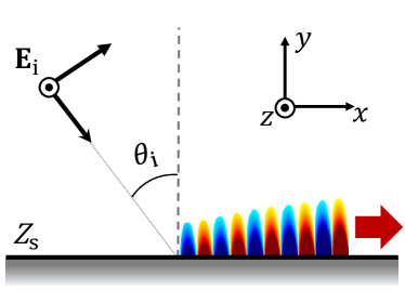
Figure 1: Boundary problem of plane wave to surface wave conversion.

Figure 1 illustrates the problem under consideration, perfect conversion (no dissipation or scattering losses) of a TE-polarized incident plane wave into a TM-polarized surface wave bound to an impenetrable metasurface in the $xz$-plane, characterized by the matrix surface impedance $\overline{\overline{Z}}_{\rm s}$. Polarization transformation is applied here to avoid field and power interference of propagating and surface waves with each other Asadchy et al. (2016). Both fields are invariant with respect to $z$. The design objective is to find $\overline{\overline{Z}}_{\rm s}$ that enables this transformation. The most desirable solution is a point-wise lossless metasurface, such that the normal component of the total Poynting vector is zero at all points of the surface. In this case, the impedance matrix is skew-Hermitian: $\overline{\overline{Z}}_{\text{s}}^{\dagger}=-\overline{\overline{Z}}_{\text{s}}$. In the special case of reciprocal surfaces, all components of the surface impedance matrix of lossless boundaries are purely imaginary Pozar (2005).

Both the incident fields and the scattered surface-wave fields must satisfy Maxwell’s equations in the upper half-space, which is assumed to be free space. To fully understand the concept of energy transfer and its further flow along the surface, a point-wise lossless discretized surface should be considered (Figure 2). The uniform amount of power carried by the incident wave (denoted as ${\bf P}_{\rm i}$ in Fig. 2) is added at each consecutive small interval. Therefore, the power carried by the surface wave should grow linearly along the surface, to satisfy the energy conservation.

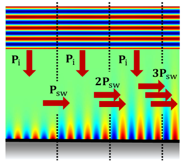
Figure 2: Illustration of a linear power growth required by the energy conservation law.

In search of a surface-wave solution that satisfies the necessary spatial power dependence, both separable and non-separable solutions to the Helmholtz equation have been considered. Conventional separable solutions are plane waves which exponentially grow along the surface. Using an $e^{j\omega t}$ time convention assumed and suppressed for time-harmonic analysis at an angular frequency $\omega$, the non-separable solutions in Cartesian coordinates Moseley (1965); Schoonaert and Luypaert (1973) allow the $z$-component of the magnetic field in TM polarization of the form

$$H_{z}=H_{0}(k_{y}x-k_{x}y)e^{-j(k_{x}x+k_{y}y)},$$ (1)

where $H_{0}$ is a constant. The wavenumbers in the $x$- and $y$-directions, $k_{x}$ and $k_{y}$, satisfy the free-space dispersion relation:

$$k_{x}^{2}+k_{y}^{2}=k_{0}^{2},$$ (2)

where $k_{0}$ is the free-space wavenumber. An evanescent wave in the $y$-direction is associated with the condition $k_{x}>k_{0}$. It is found that the time-average power carried in the $x$-direction increases quadratically with $x$. Hence, both separable and the non-separable (1) eigenwave field solutions cannot represent the surface wave converted from the incident plane wave. In other words, Maxwell’s equations in homogeneous media do not allow ideal conversion of uniform propagating plane waves into one surface wave with the use of point-wise lossless metasurfaces. Therefore, we introduce approximate nearly perfect solutions and explore possibilities offered by active/lossy and strongly non-local metasurfaces.

III Separable field solutions

Let us consider a separable solution for the surface wave, whose magnetic field is expressed as

$$\mathbf{H}^{\text{sw}}=\hat{z}H^{\text{sw}}_{z}(x,y)=\hat{z}X(x)Y(y),$$ (3)

where $X(x)$ and $Y(y)$ are functions of $x$ and $y$ only, respectively. The surface wave field component satisfies the homogeneous wave equation, $(\nabla^{2}+k_{0}^{2})H^{\text{sw}}_{z}=0$. Following the standard separation-of-variables technique Harrington (2001), one obtains a solution of the form

$$H^{\text{sw}}_{z}=H^{\text{sw}}_{0}e^{-j(k^{\prime}_{x}x+k^{\prime}_{y}y)}$$ (4)

with an arbitrary complex amplitude $H^{\text{sw}}_{0}$. The wavenumbers $k^{\prime}_{x}$, $k^{\prime}_{y}$ satisfy (2). The prime symbol denotes spectral variables.

Let us write the wavenumbers in terms of real-valued propagation ($\beta$’s) and attenuation ($\alpha$’s) constants as $k^{\prime}_{x}=\beta^{\prime}_{x}-j\alpha^{\prime}_{x}$, $k^{\prime}_{y}=\beta^{\prime}_{y}-j\alpha^{\prime}_{y}$. Because perfect transformation into a single surface mode using point-wise lossless surfaces is not possible, we consider the general solution for $H^{\text{sw}}_{z}$ in $y\geq 0$ as a superposition of (4) over the entire complex-$k_{x}$ plane, written as a two-dimensional (2-D) inverse Fourier transform

$$H^{\text{sw}}_{z}=\frac{1}{4\pi^{2}}\iint\limits_{-\infty}^{\infty}\tilde{H}^{\text{sw}}_{z}(k^{\prime}_{x},k^{\prime}_{y})e^{-j(k^{\prime}_{x}x+k^{\prime}_{y}y)}d\alpha^{\prime}_{x}d\beta^{\prime}_{x},$$ (5)

where $\tilde{H}^{\text{sw}}_{z}(k^{\prime}_{x},k^{\prime}_{y})$ is the 2-D spectrum of $H^{\text{sw}}_{z}(x,y)$. In (5), the complex propagation constant $k^{\prime}_{y}$ is found from the free-space dispersion relation (2). The branch of the square root for $\alpha^{\prime}_{y}$ is determined such that $\beta^{\prime}_{y}\geq 0$, i.e., all scattered wave components propagate away from the $y=0$ boundary. Equation (5) represents superposition of homogeneous and inhomogeneous plane waves. For (5) to represent a surface wave bound to the $xz$-plane, $\tilde{H}^{\text{sw}}_{z}(k^{\prime}_{x},k^{\prime}_{y})$ can be non-zero only in the range $\alpha^{\prime}_{y}>0$. If we desire that the converted surface wave propagates in the $+x$-axis direction along the surface, the valid region of non-zero $\tilde{H}^{\text{sw}}_{z}(k^{\prime}_{x},k^{\prime}_{y})$ in the complex-$k_{x}$ plane corresponds to $\beta^{\prime}_{x}>k_{0}$.

Using Maxwell’s equations, expressions for the E-field components of the surface wave, $\mathbf{E}^{\text{sw}}=\hat{x}E^{\text{sw}}_{x}+\hat{y}E^{\text{sw}}_{y}$, are found to be

$$E^{\text{sw}}_{x} = -\frac{1}{4\pi^{2}}\iint\limits_{-\infty}^{\infty}\frac{\eta_{0}k^{\prime}_{y}}{k_{0}}\tilde{H}^{\text{sw}}_{z}e^{-j(k^{\prime}_{x}x+k^{\prime}_{y}y)}d\alpha^{\prime}_{x}d\beta^{\prime}_{x},$$ (6)

$$E^{\text{sw}}_{y} = \frac{1}{4\pi^{2}}\iint\limits_{-\infty}^{\infty}\frac{\eta_{0}k^{\prime}_{x}}{k_{0}}\tilde{H}^{\text{sw}}_{z}e^{-j(k^{\prime}_{x}x+k^{\prime}_{y}y)}d\alpha^{\prime}_{x}d\beta^{\prime}_{x},$$ (7)

where $\eta_{0}\approx 377~{}\Omega$ is the free-space intrinsic impedance. With the general expression of the surface wave fields in (5)–(7), the surface wave design reduces to finding $\tilde{H}^{\text{sw}}_{z}$ that performs the following functions: 1) elimination of a reflected plane wave from the surface and 2) linear growth of the surface-wave power with respect to $x$ that is consistent with perfect conversion from the incident plane wave.

IV Approximate design employing a single surface wave of slow exponential growth

It is expected that there are many possibilities for the spectrum $\tilde{H}^{\text{sw}}_{z}(k_{x}^{\prime},k_{y}^{\prime})$ that satisfy the design requirements. In order to reduce the design complexity, let us consider the special case of a single spatial harmonic, such that the surface wave spectrum is represented as

$$\tilde{H}^{\text{sw}}_{z}(k_{x}^{\prime},k_{y}^{\prime})=4\pi^{2}H^{\text{sw}}_{0}\delta(k_{x}^{\prime}-k_{x})\delta(k_{y}^{\prime}-k_{y}),$$ (8)

where $H^{\text{sw}}_{0}$ is a complex amplitude and $k_{x}=\beta_{x}-j\alpha_{x}$, $k_{y}=\beta_{y}-j\alpha_{y}$ are complex propagation constants of choice in the $x$- and $y$-axis directions, respectively. The associated surface-wave field expressions are given by

$$\mathbf{H}^{\text{sw}} = \hat{z}H^{\text{sw}}_{0}e^{-(\alpha_{x}+j\beta_{x})x}e^{-(\alpha_{y}+j\beta_{y})y},$$ (9)

$$\mathbf{E}^{\text{sw}} = \left[-\hat{x}\left(\beta_{y}-j\alpha_{y}\right)+\hat{y}\left(\beta_{x}-j\alpha_{x}\right)\right]\frac{\eta_{0}H^{\text{sw}}_{0}}{k_{0}}$$ (10)

$$\times e^{-(\alpha_{x}+j\beta_{x})x}e^{-(\alpha_{y}+j\beta_{y})y}.$$

Obviously, the power carried by this simple single-mode surface wave grows exponentially along $x$, while the ideal conversion of an incident propagating plane wave into this surface wave implies linear power increase. However, solutions with a slow exponential growth can approximate the required linear law.

For complex propagation constants $k_{x}$ and $k_{y}$, the free-space dispersion relation (2) gives two separate equations for real-valued parameters $\alpha_{x}$, $\beta_{x}$, $\alpha_{y}$, and $\beta_{y}$ defined by

$$\beta_{x}^{2}+\beta_{y}^{2}-\alpha_{x}^{2}-\alpha_{y}^{2}=k_{0}^{2},$$ (11)

$$\alpha_{x}\beta_{x}+\alpha_{y}\beta_{y}=0.$$ (12)

Any combination of real values for the four parameters that satisfy (11)–(12) produce fields that satisfy Maxwell’s equations in the range $y>0$ in Fig. 1. Here, we choose $\alpha_{x}$ to be a small negative quantity and $\beta_{x}>k_{0}$. This results in $\alpha_{y}>0$, $0<\beta_{y}<k_{0}$. Such a wave represents a propagating wave of slow exponential growth in the $+x$-axis direction. Yet, the wave does not reach $y\to+\infty$, bound to the $xz$-plane, owing to $\alpha_{y}>0$.

For realization of the wave converter as a point-wise lossless non-transparent metasurface, the resulting total fields, given as a superposition of the incident plane wave and the slowly-growing surface wave, must have zero net power across the $xz$-plane everywhere Kwon and Tretyakov (2017). This condition is analogous to the local power conservation requirement for passive, lossless realization of $\Omega$-bianisotropic metasurfaces for wave transformation Epstein and Eleftheriades (2016). The total power density along the normal to the surface may be dependent on the vertical coordinate and be inhomogeneous, but we require it to be equal zero on the lossless metasurface boundary ($y=0$). This assures that all the illuminating power of the incident wave is “accepted” by the surface and consequently used for surface wave creation. For simplicity, let us consider a normally incident plane wave in Fig. 1 with the fields given by

$$\mathbf{E}^{i}=\hat{z}E^{i}_{0}e^{jk_{0}y},\ \ \mathbf{H}^{i}=-\hat{x}\frac{E^{i}_{0}}{\eta_{0}}e^{jk_{0}y}.$$ (13)

On the surface $(y=0)$, the zero net power penetration condition reads

$$\begin{split}S_{y}(x,y=0)&=S^{\rm i}_{y}+S^{\rm sw}_{y}\\ &=-{{|E_{0}|^{2}}\over{2\eta_{0}}}+{{\eta_{0}\beta_{y}}\over{2k_{0}}}|H^{\rm sw}_{0}|^{2}\,e^{-2\alpha_{x}x}=0,\end{split}$$ (14)

where $S^{\rm i}_{y}$ and $S^{\text{sw}}_{y}$ are the normal components of the time-average Poynting vector associated with the incident plane wave and the surface wave, respectively. The normal component of the Poynting vector for the total fields, $S_{y}$, is an algebraic sum because the two sets of fields are of orthogonal polarizations. Hence, for the surface wave fields (9)–(10) to cancel the incident power density on the surface, the magnetic field magnitude of the surface wave must satisfy

$$|H^{\text{sw}}_{0}|=\frac{|E_{0}|}{\eta_{0}}\sqrt{\frac{k_{0}}{\beta_{y}}}e^{\alpha_{x}x}.$$ (15)

The phase of $H^{\text{sw}}_{0}$ relative to $E_{0}$ can be arbitrary. However, if $H^{\text{sw}}_{0}$ satisfies (15), the surface wave amplitude does not grow along the surface, and, moreover, the complex amplitude should be a constant to satisfy Maxwell’s equation. Therefore, it is concluded that (14) cannot be satisfied for all $x$. In fact, (14) can be exactly satisfied only at one location in $x$ because $\alpha_{x}\neq 0$ .

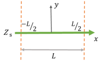
Figure 3: Illustration of the finite interval of the impenetrable surface with length $L$.

Since an exponential function either diverges or approaches zero as $x\to\pm\infty$, we can only consider approximate satisfaction of (15) over a finite interval. Consider an interval of length $L$ centered at $x=0$, as shown in Fig. 3. We can select the value of $\alpha_{x}$ such that $e^{\alpha_{x}x}$ can be considered approximately equal to unity over $-L/2<x<L/2$. In other words, attenuating constant $\alpha_{x}$ and length $L$ should be balanced to satisfy the condition $|\alpha_{x}L|\ll 1$. Picking the middle point of the $x$-range at $x=0$ for exact enforcement of (15) and setting the phase of $H^{\text{sw}}_{0}$ equal to that of $E_{0}$, we assign

$$|H^{\text{sw}}_{0}|=\frac{E_{0}}{\eta_{0}}\sqrt{\frac{k_{0}}{\beta_{y}}}.$$ (16)

The $x$-component of the time-average Poynting vector of the surface wave is equal to

$$S_{x}=\frac{1}{2}\text{Re}\{E^{\text{sw}}_{y}\times H^{\text{sw}*}_{z}\}=\frac{\eta_{0}\beta_{x}}{2k_{0}}|H^{\text{sw}}_{0}|^{2}e^{-2(\alpha_{x}x+\alpha_{y}y)}.$$ (17)

Integrating $S_{x}(x,y)$ over $0<y<\infty$, we find that the power propagating in the $+x$-direction per unit length in $z$ to be

$$P_{x}=\frac{\eta_{0}\beta_{x}}{4k_{0}\alpha_{y}}|H^{\text{sw}}_{0}|^{2}e^{-2\alpha_{x}x}\approx\frac{\eta_{0}\beta_{x}}{4k_{0}\alpha_{y}}|H^{\text{sw}}_{0}|^{2}(1-2\alpha_{x}x).$$ (18)

Equation (18) shows that the power carried by the surface wave increases approximately linearly with $x$, as desired. In addition, the rate of power increase with respect to $x$—$dP_{x}/dx$—is equal to the power density of the incident plane wave.

A surface of finite length $L$ is expected to convert the power of the illuminating plane wave falling on the given range, $-L/2<x<L/2$, into a growing surface wave propagating in the $+x$-axis direction. We note that the surface wave field values at the starting point of the surface $(x=-L/2)$ is not zero. This means that the wave-converting surface needs an input power at $x=-L/2$ in an eigenmode characterized by a damped oscillatory function in $y$ to perform the desired wave conversion, but there is no input power if the considered section of length $L$ has no continuation at $x<-L/2$. For this reason, for numerical validation of the designed surfaces in Section VI, performance of the wave converting surfaces is evaluated without an input surface wave as well.

V Surface Impedance Characterization of the Coupler

To ascertain which type of a surface is needed for the transformation described in the previous section, we consider the boundary condition at $y=0$ in the form of a surface impedance. Using superposition, the total tangential fields on the surface are found from (9)–(10) and (13) to be

$$\mathbf{E}_{\rm t} = \hat{z}E_{{\rm t}z}+\hat{x}E_{{\rm t}x}=\hat{z}E_{0}-\hat{x}H^{\text{sw}}_{0}\frac{k_{y}\eta_{0}}{k_{0}}e^{-jk_{x}x},$$ (19)

$$\mathbf{H}_{\rm t} = \hat{z}H_{{\rm t}z}+\hat{x}H_{{\rm t}x}=\hat{z}H^{\rm sw}_{0}e^{-jk_{x}x}-\hat{x}\frac{E_{0}}{\eta_{0}},$$ (20)

where $E_{{\rm t}z}$ and $E_{{\rm t}x}$ are the tangential electric field components derived from the incident and reflected (quasi-surface) waves. The magnetic field components $H_{{\rm t}x}$ and $H_{{\rm t}z}$ are denoted similarly. Now, the $y=0$ surface can be characterized with a surface impedance tensor $\overline{\overline{Z}}_{\text{s}}$, which relates $\mathbf{E}_{\text{t}}$ and the induced surface current $\mathbf{J}_{\text{s}}=\hat{y}\times\mathbf{H}_{\text{t}}$ via

$$\mathbf{E}_{\text{t}}=\overline{\overline{Z}}_{\text{s}}\cdot\mathbf{J}_{\text{s}}=\begin{bmatrix}Z_{xx}&Z_{xz}\\ Z_{zx}&Z_{zz}\end{bmatrix}\mathbf{J}_{\text{s}},$$ (21)

where $Z_{xx}$, $Z_{xz}$, $Z_{zx}$, and $Z_{zz}$ are terms of the anisotropic $2\times 2$ matrix $\overline{\overline{Z}}_{\rm s}$. The two complex-valued equations in terms of field quantities are

$$\begin{array}[]{l}\displaystyle E_{{\rm t}x}=Z_{xx}H_{{\rm t}z}-Z_{xz}H_{{\rm t}x},\\ E_{{\rm t}z}=Z_{zx}H_{{\rm t}z}-Z_{zz}H_{{\rm t}x}.\end{array}$$ (22)

Each of the four matrix elements can be represented as a complex number, i.e.,

$$\overline{\overline{Z}}_{\text{s}}=\begin{bmatrix}R_{xx}+jX_{xx}&R_{xz}+jX_{xz}\\ R_{zx}+jX_{zx}&R_{zz}+jX_{zz}\end{bmatrix},$$ (23)

where the $R$ and $X$ quantities are real-valued and represent the resistance and reactance parts of the associated impedance values. Since there are two complex-valued equations in (22) for four complex-valued impedance elements, the solution is not unique and thus there is a freedom that can be exploited for setting their values. Equating the real and imaginary parts on the two sides of (22), we obtain four real-valued equations. They can be expressed as a matrix equation in a compact form as

$$\begin{bmatrix}R_{xx}&R_{xz}\\ R_{zx}&R_{zz}\end{bmatrix}\begin{bmatrix}{\rm Re}\{H_{\text{t}z}\}&{\rm Im}\{H_{\text{t}z}\}\\ -{\rm Re}\{H_{\text{t}x}\}&-{\rm Im}\{H_{\text{t}x}\}\end{bmatrix}+\begin{bmatrix}X_{xx}&X_{xz}\\ X_{zx}&X_{zz}\end{bmatrix}\begin{bmatrix}-{\rm Im}\{H_{\text{t}z}\}&{\rm Re}\{H_{\text{t}z}\}\\ {\rm Im}\{H_{\text{t}x}\}&-{\rm Re}\{H_{\text{t}x}\}\end{bmatrix}=\begin{bmatrix}{\rm Re}\{E_{\text{t}x}\}&{\rm Im}\{E_{\text{t}x}\}\\ {\rm Re}\{E_{\text{t}z}\}&{\rm Im}\{E_{\text{t}z}\}\end{bmatrix}.$$ (24)

Depending on requirements on loss and reciprocity of the system, different constraints can be placed on the values of the resistance and reactance parts of the tensor elements and the associated impedance/admittance matrices can be found from (24). A reciprocal system is characterized by a symmetric matrix, i.e., $\overline{\overline{Z}}_{\text{s}}^{T}=\overline{\overline{Z}}_{\text{s}}$. As to losses in the system, a point-wise lossless system is characterized by a skew-Hermitian matrix, i.e., $\overline{\overline{Z}}_{\rm s}^{\dagger}=-\overline{\overline{Z}}_{\rm s}$. In the following, we discuss solutions for $\overline{\overline{Z}}_{\text{s}}$ for reciprocal/non-reciprocal and lossless/active-lossy combinations.

V.1 Reciprocal and point-wise lossless

Let us first describe the most desirable case from the practical point of view, when the system is reciprocal and lossless at every point. All the elements of the impedance matrix are purely imaginary and the matrix is skew-Hermitian: $Z_{xx}=jX_{xx}$, $Z_{xz}=Z_{zx}=jX_{xz}$, and $Z_{zz}=jX_{zz}$. There are three real-valued parameters ($X_{xx}$, $X_{xz}$, and $X_{zz}$), while there are four linear equations in (24).

V.1.1 Periodic approximation

One can solve all four equations exactly in the case of magnetic field magnitude described by (15). The solutions for the impedance matrix as well as the associated admittance matrix are found to be

$$\overline{\overline{Z}}_{\rm s}=j\begin{bmatrix}\displaystyle\frac{\eta_{0}}{k_{0}}\left(\alpha_{y}-\beta_{y}\cot\beta_{x}x\right)&\displaystyle\frac{\eta_{0}}{\sin\beta_{x}x}\sqrt{\frac{\beta_{y}}{k_{0}}}\\ \displaystyle\frac{\eta_{0}}{\sin\beta_{x}x}\sqrt{\frac{\beta_{y}}{k_{0}}}&-\eta_{0}\cot\beta_{x}x\end{bmatrix},$$ (25)

$$\overline{\overline{Y}}_{\rm s}=\frac{j}{D}\begin{bmatrix}-\eta_{0}\cot\beta_{x}x&\displaystyle-\frac{\eta_{0}}{\sin\beta_{x}x}\sqrt{\frac{\beta_{y}}{k_{0}}}\\ \displaystyle-\frac{\eta_{0}}{\sin\beta_{x}x}\sqrt{\frac{\beta_{y}}{k_{0}}}&\displaystyle\frac{\eta_{0}}{k_{0}}\left(\alpha_{y}-\beta_{y}\cot\beta_{x}x\right)\end{bmatrix},$$ (26)

where $D$ is the determinant of $\overline{\overline{Z}}_{\text{s}}$ and is equal to $D=\eta_{0}^{2}\left(\alpha_{y}\cot\beta_{x}x+\beta_{y}\right)/k_{0}$. This solution describes a completely lossless structure, but the fields satisfy Maxwell’s equations exactly only when $e^{\alpha_{x}x}$ approaches unity.

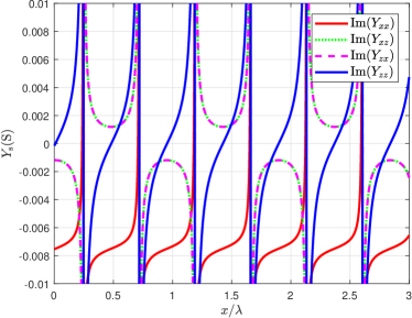
Figure 4: Susceptance elements of the surface admittance $Y_{\rm s}$ for the reciprocal and lossless periodic approximation (26) with $\alpha_{x}=-0.0083k_{0}$, $\alpha_{y}=0.3524k_{0}$, $\beta_{x}=1.06k_{0}$, and $\beta_{y}=0.025k_{0}$.

For an example set of complex propagation constants (their values are shown in the caption), Fig. 4 plots the susceptance elements of $\overline{\overline{Y}}_{\text{s}}$ (26). The propagation constants are chosen for a surface of length $L=20\lambda_{0}$. Along the $+x$-axis direction, a moderately slow exponential growth was chosen with $|\alpha_{x}L|\ll 1$ and a propagation constant just outside the visible (propagating) range was selected as $\beta_{x}=1.06k_{0}$. The associated values of $\alpha_{y}$, $\beta_{y}$ are found from (11)–(12). The admittance tensor parameters are found to be periodic functions with period $2\pi/\beta_{x}$. Furthermore, all four parameters diverge when $D=0$, or at $x=(1/\beta_{x})[-\cot^{-1}(\beta_{y}/\alpha_{y})+n\pi]$ $(n=0,\pm 1,\pm 2,\ldots)$.

V.1.2 Least squares approximation

To find an approximation for the surface impedance/admittance of a lossless and reciprocal surface, which creates the fields that satisfy Maxwell’s equations, the least squares approximation Strang (2016) can be used. The amplitude of the magnetic field of the surface wave in this case is defined as (16). In terms of the vector with three reactance elements to be determined, $\mathbf{X}=\begin{bmatrix}X_{xx}&X_{xz}&X_{zz}\end{bmatrix}^{T}$, the four linear equations (24) can be rewritten as

$$\bar{\bar{H}}_{\text{t}}\mathbf{X}=\mathbf{E}_{t},$$ (27)

where

$$\bar{\bar{H}}_{\rm t} = \begin{bmatrix}-{\rm Im}\{H_{{\rm t}z}\}&{\rm Im}\{H_{{\rm t}x}\}&0\\ {\rm Re}\{H_{{\rm t}z}\}&-{\rm Re}\{H_{{\rm t}x}\}&0\\ 0&-{\rm Im}\{H_{{\rm t}z}\}&{\rm Im}\{H_{{\rm t}x}\}\\ 0&{\rm Re}\{H_{{\rm t}z}\}&-{\rm Re}\{H_{{\rm t}x}\}\end{bmatrix},$$ (28)

$$\mathbf{E}_{t} = \begin{bmatrix}{\rm Re}\{E_{{\rm t}x}\}&{\rm Im}\{E_{{\rm t}x}\}&{\rm Re}\{E_{{\rm t}z}\}&{\rm Im}\{E_{{\rm t}z}\}\end{bmatrix}^{T}.$$ (29)

This overdetermined system cannot be exactly satisfied, other than the case in Sec. V.1.1. The least squares solution solves for $\mathbf{X}$ such that the error defined by

$$\text{error}=\lVert\mathbf{E}_{t}-\bar{\bar{H}}_{\text{t}}\mathbf{X}\rVert^{2}$$ (30)

is minimized. The solution is given by Strang (2016)

$$\mathbf{X}=\left(\bar{\bar{H}}_{\text{t}}^{T}\bar{\bar{H}}_{\text{t}}\right)^{-1}\bar{\bar{H}}_{\text{t}}^{T}\mathbf{E}_{t}.$$ (31)

The resulting admittance profile in this case is generally aperiodic, and the susceptance elements of $\overline{\overline{Y}}_{\text{s}}$ are shown in Figure 5. The behavior of the admittance curves in both approximations, periodic and least squares, are similar, but differences become pronounced at locations far from $x=0$.

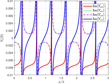
Figure 5: Susceptance elements of the surface admittance $Y_{\rm s}$ for the reciprocal and lossless least squares approximation with $\alpha_{x}=-0.0083k_{0}$, $\alpha_{y}=0.3524k_{0}$, $\beta_{x}=1.06k_{0}$, and $\beta_{y}=0.025k_{0}$.

An alternative approximate solution which introduces non-reciprocity while the system remains lossless at all points can be found in a similar way, but it does not offer any advantages in possible realizations.

V.2 Reciprocal and active/lossy

A possible way to find an exact solution which satisfies Maxwell’s equations is to mitigate the condition for absence of losses or gain everywhere at the metasurface plane. In other words, strong non-local response in metasurface is allowed. One of the reciprocal and active/lossy solutions which satisfy (16) identically at all points of the metasurface is described by the impedance matrix with imaginary diagonal elements elements and complex off-diagonal elements. The impedance matrix and the associated admittance matrix are found to be

$$\overline{\overline{Z}}_{\rm s}=\begin{bmatrix}j\displaystyle{X_{xx}}&\hskip 14.22636pt\displaystyle{R_{xz}+jX_{xz}}\\ \displaystyle{R_{xz}+jX_{xz}}&\displaystyle{jX_{zz}}\end{bmatrix},$$ (32)

$$\overline{\overline{Y}}_{\rm s}=\displaystyle{1\over D}\begin{bmatrix}j\displaystyle{X_{zz}}&-(\displaystyle{R_{xz}+jX_{xz}})\\ -(\displaystyle{R_{xz}+jX_{xz}})&\hskip 14.22636ptj\displaystyle{X_{xx}}\end{bmatrix},$$ (33)

where

$$X_{xx}={\eta_{0}\over k_{0}}\,\left(\alpha_{y}-\beta_{y}\cot\beta_{x}x\right)+{\eta_{0}\beta_{y}\left(1-e^{2\alpha_{x}x}\right)\over 2k_{0}\cos{\beta_{x}x}\sin{\beta_{x}x}},$$ (34)

$$R_{xz}={\eta_{0}\over 2\cos\beta_{x}x}\sqrt{\beta_{y}\over k_{0}}\left(e^{\alpha_{x}x}-e^{-\alpha_{x}x}\right),$$ (35)

$$X_{xz}={\eta_{0}\over 2\sin{\beta_{x}x}}\sqrt{\beta_{y}\over k_{0}}\left(e^{\alpha_{x}x}+e^{-\alpha_{x}x}\right),$$ (36)

$$X_{zz}={\eta_{0}\over 2}\left(\tan{\beta_{x}x}-\cot{\beta_{x}x}-{e^{-2\alpha_{x}x}\over\cos{\beta_{x}x}\sin{\beta_{x}x}}\right),$$ (37)

and $D=-X_{xx}X_{zz}-(R_{xz}+jX_{xz})^{2}$ is the determinant of $\overline{\overline{Z}}_{\text{s}}$.

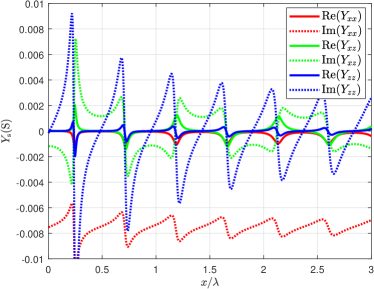
Figure 6: Surface admittance $Y_{\rm s}$ for the reciprocal and active/lossy case with $\alpha_{x}=-0.0083k_{0}$, $\alpha_{y}=0.3524k_{0}$, $\beta_{x}=1.06k_{0}$, $\beta_{y}=0.025k_{0}$. All the components of the admittance are complex numbers.

Figure 6 plots the elements of $\overline{\overline{Y}}_{\text{s}}$ for the same example set of complex propagation constants considered in previous subsections. All the admittance terms are complex in contrary to the impedance terms due to the fact that the determinant $D$ is a complex number. The admittance tensor parameters are found to be aperiodic functions.

This revealed possibility to find an exact solution in form of only one incident propagating plane wave and one surface mode (with the amplitude given by (16)) using active/lossy metasurfaces reminds of the analogous property of perfect anomalous reflectors which transform one incident plane wave into only one reflected plane wave propagating in the desired direction Asadchy et al. (2016); Estakhri and Alù (2016); Epstein and Eleftheriades (2016); Díaz-Rubio et al. (2017). We expect that also in the case of considered transformation into a single surface mode, realizations can be found in form of non-local metasurfaces, where “active” regions work as receiving leaky-wave antennas while the “lossy” regions as transmitting antennas, in analogy with the approach presented in Díaz-Rubio et al. (2017). In contrast to transformers of propagating waves which are periodically modulated surfaces, in this case the receiving surface is divided into two regions, the first of which is receiving power (effective loss) and the second one is radiating power (effective gain), as is seen from formula (14) with a constant value of $|H^{\rm sw}_{0}|$. The parameters of the metasurface can be chosen so that these two powers are equal, so that overall the structure is lossless.

It is stressed that realizations of such non-local metasurfaces which emulate active/lossy response do not require active elements. Basically, the non-local metasurface does not act as a boundary at every point: In the “lossy” region part of the input power is accepted by auxiliary waves which exist inside the metasurface device, and this power is used to enhance the generated plane wave in the “active” region. Actually, any reactive impedance boundary (except perfect electric conductor) models some fields behind the surface, only in the point-wise lossless case all the power which is accepted at a given point is reflected back at the same point, without any power transport along the metasurface plane. In the non-local scenario, some power also moves inside the metasurface in the direction of power growth of the generated plane wave.

V.3 Non-reciprocal and locally active/lossy

By introducing non-reciprocity in addition to effective loss and gain, one can find more elegant exact solutions which satisfy Maxwell’s equations, corresponding to creation of a single surface wave with the amplitude (16). It can be described by a non-Hermitian impedance matrix with all the elements being purely imaginary: $Z_{xx}=jX_{xx}$, $Z_{xz}=jX_{xz}$, $Z_{zx}=jX_{zx}$, $Z_{zz}=jX_{zz}$. The solution for the impedance matrix as well as the associated admittance matrix are found to be

$$\overline{\overline{Z}}_{\rm s}=j\begin{bmatrix}\@add@centering\centering\displaystyle{\eta_{0}\over k_{0}}\left(\alpha_{y}-\beta_{y}\cot{\beta_{x}x}\right)&\hskip 14.22636pt\displaystyle{\eta_{0}\over\sin{\beta_{x}x}}{\displaystyle\sqrt{\beta_{y}\over k_{0}}}e^{-\alpha_{x}x}\\ \displaystyle{\eta_{0}\over\sin{\beta_{x}x}}{\displaystyle\sqrt{\beta_{y}\over k_{0}}}e^{\alpha_{x}x}&-\eta_{0}\cot{\beta_{x}x}\end{bmatrix},$$ (38)

$$\overline{\overline{Y}}_{\rm s}=\displaystyle{j\over D}\begin{bmatrix}-\eta_{0}\cot{\beta_{x}x}&\displaystyle-{\eta_{0}\over\sin{\beta_{x}x}}{\displaystyle\sqrt{\beta_{y}\over k_{0}}}e^{-\alpha_{x}x}\\ \displaystyle-{\eta_{0}\over\sin{\beta_{x}x}}{\displaystyle\sqrt{\beta_{y}\over k_{0}}}e^{\alpha_{x}x}&\hskip 14.22636pt\displaystyle{\eta_{0}\over k_{0}}\left(\alpha_{y}-\beta_{y}\cot{\beta_{x}x}\right)\end{bmatrix},$$ (39)

where $D$ is the determinant of $\overline{\overline{Z}}_{\text{s}}$ and is equal to $D=\eta_{0}^{2}\left(\alpha_{y}\cot\beta_{x}x+\beta_{y}\right)/k_{0}$.

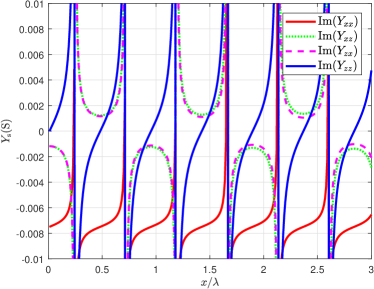
Figure 7: Surface admittance $Y_{\rm s}$ for the non-reciprocal and active/lossy case with $\alpha_{x}=-0.0083k_{0}$, $\alpha_{y}=0.3524k_{0}$, $\beta_{x}=1.06k_{0}$, $\beta_{y}=0.025k_{0}$. All the components are purely imaginary.

Figure 7 plots the elements of the susceptance elements of $\overline{\overline{Y}}_{\text{s}}$ for the same example set of complex propagation constants considered in Sec. V.1. The admittance tensor parameters are found to be aperiodic functions and all four parameters diverge when $D=0$, or at $x=(1/\beta_{x})[-\cot^{-1}(\beta_{y}/\alpha_{y})+n\pi]$ $(n=0,\pm 1,\pm 2,\ldots)$. It is observed that the off-diagonal terms are the same at $x=0$ and they slowly diverge from each other away from $x=0$. Therefore, realization of such surface is expected to be a difficult and probably non-profitable task, compared to reciprocal structures. However, they remain close to each other in the $x$-range considered, signifying that the degree of non-reciprocity and active/lossy property is not significant. Also as expected, the parameters in Fig. 7 are close to those of the reciprocal and lossless case shown in Fig. 4.

By using the aforementioned surface impedance profiles, one can simulate and, further, realize the necessary surface to convert a propagating plane wave into a quasi-surface wave with high efficiency.

VI Numerical results

Using full-wave simulations with COMSOL Multiphysics com , the conversion characteristics of the surfaces in Sec. V can be evaluated. The model is a rectangular cross section in the $xy$-plane with a length $L=20\lambda_{0}$ and a height $H=5\lambda_{0}$. Impedance boundary conditions are impenetrable and applied to the surface by impressing an electric surface current specified in terms of the tangential electric field and the surface admittance matrix (in our case $J_{x}=Y_{xx}E_{{\rm t}x}+Y_{xz}E_{{\rm t}z}$ and $J_{z}=Y_{zx}E_{{\rm t}x}+Y_{zz}E_{{\rm t}z}$). In this work we consider two cases: imitation of an infinitely long surface with an input surface wave using two surface-wave ports and a model of the initial portion of the wave-converting surface with no input surface-wave port (i.e., one surface-wave port for the converted output power). The used frequency is $f=10$ GHz, but the results are scalable to any frequency.

VI.1 Model with an input surface wave

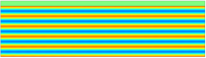
(a)

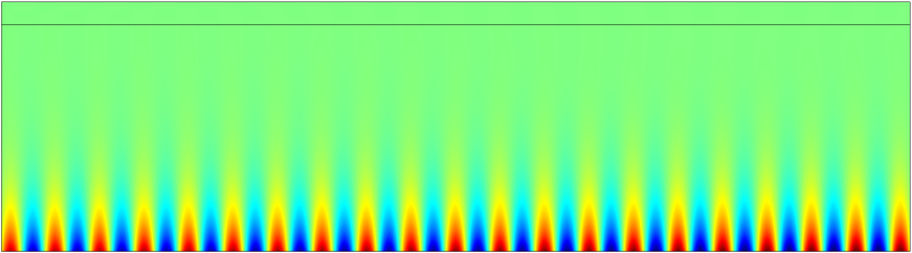
(b)

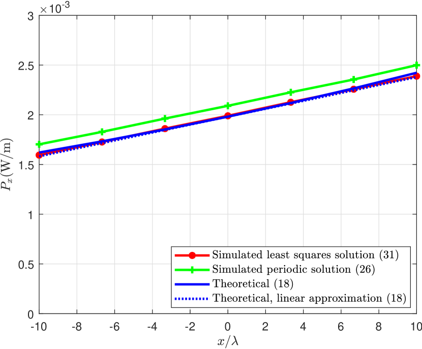
(c)

Figure 8: (a) Field distribution of the tangential component of the total field, $E_{z}$, in the lossless and reciprocal design (least squares solution). The length of the surface is $L=20\lambda_{0}$, wave parameters are: $\alpha_{x}=-0.0016k_{0}$, $\alpha_{y}=0.2041k_{0}$, $\beta_{x}=1.0206k_{0}$, $\beta_{y}=0.008k_{0}$. (b) Simulated $H_{z}$ field distribution in the lossless and reciprocal design (least squares solution). Conversion efficiency is nearly $100\%$. (c) The tangential power growth along the surface for the least squares (efficiency is 99.8%), approximate periodic (efficiency is 99.6%), theoretical exponential and theoretical linear approximate solutions.

To model an $L$-long section of the infinite structure, port conditions on both sides of the box were defined. In COMSOL, the mode fields are specified to be TM-polarized and have a $y$-dependence of $e^{-(\alpha_{y}+j\beta_{y})y}$ on the port surfaces. Port 1 on the left side is a negative resistor and it pumps energy to the system to mimic the surface wave that comes from the “hidden” part of the infinite surface. This is implemented by setting the propagation constant normal to the port surface to $-(\beta_{x}-j\alpha_{x})$. Port 2 on the right side is completely passive and receives all the energy carried by a quasi-surface wave. The conversion efficiency in the case with an input power is the fraction of power carried by the surface wave that exits $x=L/2$ less the surface wave power that enters $x=-L/2$, divided by the incident power that falls on $-L/2<x<L/2$.

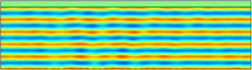
(a)

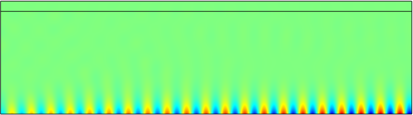
(b)

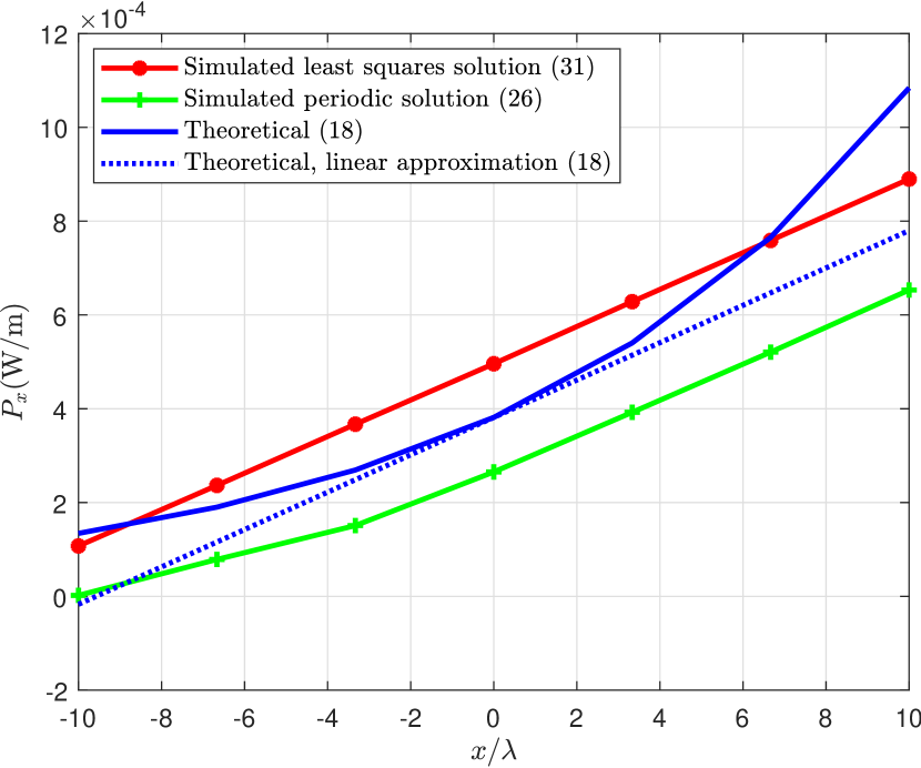
(c)

Figure 9: (a) Field distribution of the tangential component of the total field, $E_{z}$, in the lossless and reciprocal design (least squares solution). The length of the surface is $L=20\lambda_{0}$, wave parameters are: $\alpha_{x}=-0.0083k_{0}$, $\alpha_{y}=0.3524k_{0}$, $\beta_{x}=1.06k_{0}$, $\beta_{y}=0.025k_{0}$. (b) Simulated $H_{z}$ field distribution in the lossless and reciprocal design (least squares solution). The conversion efficiency is 98.4%. (c) The tangential power growth along the surface for the least squares (efficiency is 98.4%), approximate periodic (efficiency is 81.7%), theoretical exponential and theoretical linear approximate solutions.

Figure 8 demonstrates the result for a lossless and reciprocal system (specifically, the least squares solution), where the surface wave parameters are: $\alpha_{x}=-0.0016k_{0}$, $\alpha_{y}=0.2041k_{0}$, $\beta_{x}=1.0206k_{0}$, and $\beta_{y}=0.008k_{0}$. A snapshot of the $z$-component of the total E-field, $E_{z}$, is plotted in Fig. 8(a). No reflected propagating wave is visible and the total field is virtually equal to the incident field. Figure 8(b) plots a snapshot of $H_{z}$, showing a slowly growing surface wave that is bound to the $xz$-plane. Here, $\alpha_{x}$ is a small negative quantity, therefore the linear approximation of an exponential function is highly accurate and the linear growth of the tangential component of the power is smooth. In order to evaluate the wave conversion performance quantitatively, the total $+x$-directed power per unit length in $z$ [i.e., $P_{x}$ in (18)] that penetrates an $x=\text{constant}$ plane is shown in Fig. 8(c) with respect to $x$ between theory and simulation. The simulated power profiles agree well with the linear approximation of a slow exponential growth. The efficiency of such conversion is calculated to be 99.8% (least squares solution), which is practically perfect.

Figure 9 demonstrates the result for a lossless and reciprocal system (the least squares solution) when the surface wave parameters are $\alpha_{x}=-0.0083k_{0}$, $\alpha_{y}=0.3524k_{0}$, $\beta_{x}=1.06k_{0}$, and $\beta_{y}=0.025k_{0}$. A faster exponential growth was chosen compared with the previous case to investigate the characteristics. In case of $\alpha_{x}$ being a negative quantity farther away from zero, the linear approximation is not as accurate, but the efficiency is still found to be high at 98.4%, reduced only slightly from the previous case in Fig. 8. This slight drop can be understood as a consequence of a poorer approximation of a faster exponential growth to a linear growth. Reflection of the incident plane wave is minor, so that $E_{z}$ is only slightly modified from the incident field [Figure 9(a)]. We also observe that the input power (normalized to the power density of the plane wave) at $x=-L/2$ is significantly lower than in the small $|\alpha_{x}|$ case in Fig. 8.

Owing to the construction of a growing surface wave solution at a low exponential rate, a surface wave input is required for perfect conversion. Although this is an appropriate approach to the analysis of the performance of a middle section of a large receiving surface, requiring an input wave is not desirable if we consider edges of a finite-length surface. However, if the required input surface power is low as in the case shown in Fig. 9, it may still be possible to achieve a high efficiency without an input wave. This possibility is investigated next.

VI.2 Model without an input surface wave

From one side we define the “starting point” of the surface by eliminating the input surface-wave port in previous configurations and applying perfectly matched layer from the left side (the same way we can apply passive port condition, their impact here is no different). To the right side we connect a port, which receives all the energy carried by the quasi-surface wave. The conversion efficiency in the case of an absence of the input power is the fraction of power carried by the surface wave that exits $x=L/2$ relative to the incident power that falls on $-L/2<x<L/2$. It is important to note that the plane-to-surface waves conversion efficiency in the case of no input surface wave is equal to the conversion efficiency of the corresponding leaky-wave antenna Minatti et al. (2017) in a reciprocal operation as a radiator. The aperture efficiency equals 100% by design, and the radiation efficiency approaches 100% for lossless surfaces.

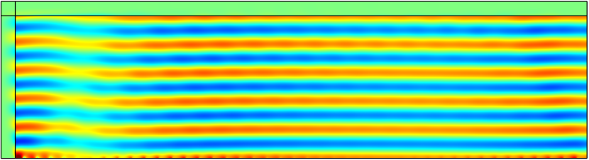
(a)

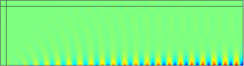
(b)

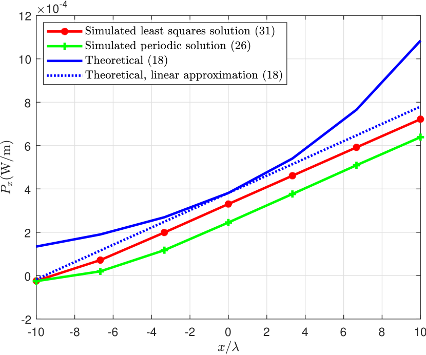
(c)

Figure 10: (a) Field distribution of the tangential component of the total field, $E_{z}$, in the lossless and reciprocal design (least squares solution). The length of the surface is $L=20\lambda_{0}$, wave parameters are: $\alpha_{x}=-0.0083k_{0}$, $\alpha_{y}=0.3524k_{0}$, $\beta_{x}=1.06k_{0}$, $\beta_{y}=0.025k_{0}$. (b) Simulated $H_{z}$ field distribution in the lossless and reciprocal design (least squares solution). The conversion efficiency is 90.5%. (c) The tangential power growth along the surface for the least squares (efficiency is 90.5%), approximate periodic (efficiency is 80.2%), theoretical exponential and theoretical linear approximate solutions.

With the same set of surface wave parameters as in Fig. 9, snapshots of the $z$-component of the total E-field, $E_{z}$, and the surface wave magnetic field distribution for the lossless and reciprocal surface design (least squares solution) are shown in Fig. 10(a) and Fig. 10(b), respectively. The power $P_{x}$ is plotted in Fig. 10(c) for the analytical and numerical results. We note that in numerical simulations the perfectly matched layer on the left side unfortunately distorts the incident plane wave, not quite adequately modelling the plane wave. Moreover, slightly negative values for the simulated power at $x=-L/2$ are due to the diffracted waves contributing to power propagating along the $-x$-direction. However, after a short transition, a steadily growing surface-wave behavior is established. Conversion efficiencies for the least squares and approximate periodic solutions are numerically found to be $90.5\%$ and $80.2\%$, respectively. These efficiencies are further reduced from the case in Fig. 9 due to the omission of the input surface wave required by the theory. This result means that the designed metasurface does not suffer from significant efficiency losses even if used without an input power. In addition, it is noted that the growing surface wave parameters shown in Fig. 10 represent one of many design possibilities. There may be other choices of $\alpha_{x}$ and $\beta_{x}$ that lead to higher efficiency values. Preliminary numerical tests show that efficiency values as high as 95% are possible for the $20\lambda$-long surface considered in this study.

VII Conclusions

In this paper the conversion of a propagating plane wave into a surface wave has been examined theoretically and numerically. In the theoretical discussion the limitations resulting from the required linear growth of the power carried by the surface wave along the direction of propagation are revealed. We have proved that for this spatial power dependence, both separable and non-separable eigenwave field solutions to the Helmholtz equations are unable to represent the surface wave converted from incident propagating plane waves, for any point-wise lossless receiving surface. Next we have shown that a properly constructed approximate separable solution with a slow exponential growth of the fields can serve as an accurate approximation of the ideally converted surface wave. Moreover, we have proposed several alternative design scenarios, leading to specific surface impedance profiles of nearly ideal wave-converting metasurfaces.

Furthermore, we have shown that dropping the requirement of local (at every point) passivity of the receiving surface potentially opens up possibilities for creation of perfect propagating/surface mode converters using non-local metasurfaces. In this new scenario, the surface first acts as a receiving leaky-wave antenna, emulating an absorbing surface. The received power is then transported along the surface and radiated into space, emulating an active surface. We expect that such locally active/lossy but overall lossless converters can be realized as carefully designed nonuniform patch arrays, generalizing the approach used in (Díaz-Rubio et al., 2017) for anomalous reflectors.

Out of the metasurface designs, the tensor surface impedance based on the least squares solution of the boundary condition and non-local metasurfaces emulating the active/lossy surface impedance allow realization using low-loss, reciprocal constituents. Arrays of printed subwavelength resonators on a grounded dielectric substrate Fong et al. (2010); Minatti et al. (2012); Patel and Grbic (2013) are prime candidates for realizing the required surface reactance tensor. In the case of non-local metasurfaces, the required active/lossy profile is realized at some electrically small distance from the patch arrays, where the auxiliary reactive fields effectively decay Díaz-Rubio et al. (2017). The position-dependent shape, size, and rotation angle of an anisotropic printed resonator are determined based on the eigenvalues and eigenvectors of the reactance tensor. Realizing a non-reciprocal surface characteristic will require constituents such as ferromagnetic components Pozar (2005) or magnetless non-reciprocal devices Kodera et al. (2013).

References

- Oliner and Jackson (2007) A. A. Oliner and D. R. Jackson, “Leaky-wave antennas,” in Antenna Engineering Handbook, edited by J. L. Volakis (McGraw-Hill, New York, 2007) 4th ed., Chap. 11.
- Monticone and Alù (2015) F. Monticone and A. Alù, “Leaky-wave theory, techniques, and applications: from microwaves to visible frequencies,” Proc. IEEE 103, 793 (2015).
- Martinez-Ros et al. (2012) A. J. Martinez-Ros, J. L. Gómez-Tornero, and G. Goussetis, “Planar leaky-wave antenna with flexible control of the complex propagation constant,” IEEE Trans. Antennas Propag. 60, 1625 (2012).
- Tierny and Grbic (2015) B. B. Tierny and A. Grbic, “Arbitrary leaky-wave antenna patterns with stacked metasurfaces,” in Proc. 2015 IEEE Antennas Propag. Soc. Int. Symp. (Vancouver, Canada, 2015) pp. 1088–1089.
- Minatti et al. (2016a) G. Minatti, F. Caminita, E. Martini, and S. Maci, “Flat optics for leaky-waves on modulated metasurfaces: adiabatic Floquet-wave analysis,” IEEE Trans. Antennas Propag. 64, 3896 (2016a).
- Minatti et al. (2016b) G. Minatti, F. Caminita, E. Martini, M. Sabbadini, and S. Maci, “Synthesis of modulated-metasurface antennas with amplitude, phase and polarization control,” IEEE Trans. Antennas Propag. 64, 3907 (2016b).
- Asadchy et al. (2016) V. S. Asadchy, M. Albooyeh, S. N. Tcvetkova, A. Díaz-Rubio, Y. Ra’di, and S. A. Tretyakov, “Perfect control of reflection and refraction using spatially dispersive metasurfaces,” Phys. Rev. B 94, 075142 (2016).
- Estakhri and Alù (2016) N. M. Estakhri and A. Alù, “Wave-front transformation with gradient metasurfaces,” Phys. Rev. X 6, 041008 (2016).
- Epstein and Eleftheriades (2016) A. Epstein and G. V. Eleftheriades, “Synthesis of passive lossless metasurfaces using auxiliary fields for reflectionless beam splitting and perfect reflection,” Phys. Rev. Lett. 117, 256103 (2016).
- Kwon and Tretyakov (2017) D.-H. Kwon and S. A. Tretyakov, “Perfect reflection control for impenetrable surfaces using surface waves of orthogonal polarization,” Phys. Rev. B 96, 085438 (2017).
- Díaz-Rubio et al. (2017) A. Díaz-Rubio, V. S. Asadchy, A. Elsakka, and S. A. Tretyakov, “From the generalized reflection law to the realization of perfect anomalous reflectors,” Sci. Adv. 3, e1602714 (2017).
- Sun et al. (2012) S. Sun, Q. He, S. Xiao, Q. Xu, X. Li, and L. Zhou, “Gradient-index meta-surfaces as a bridge linking propagating waves and surface waves,” Nat. Mater. 11, 426 (2012).
- Yu et al. (2011) N. Yu, P. Genevet, M. A. Kats, F. Aieta, J.-P. Tetienne, F. Capasso, and Z. Gaburro, “Light propagation with phase discontinuities: generalized laws of reflection and refraction,” Science 334, 333 (2011).
- Qu et al. (2013) C. Qu, S. Xiao, S. Sun, Q. He, and L. Zhou, “A theoretical study on the conversion efficiencies of gradient meta-surfaces,” EPL 101, 54002 (2013).
- Sun et al. (2016) W. Sun, Q. He, S. Sun, and L. Zhou, “High-efficiency surface plasmon meta-couplers:concept and microwave-regime realizations,” LSA 5, e16003 (2016).
- Achouri and Caloz (2016a) K. Achouri and C. Caloz, “Surface wave routing of beams by a transparent birefringent metasurface,” in Proc. 10th Int. Congress Adv. Electromagn. Mater. Microw. Opt. (Metamaterials 2016) (Crete, Greece, 2016) pp. 13–15.
- Achouri and Caloz (2016b) K. Achouri and C. Caloz, “Space-wave routing via surface waves using a metasurface system,” (2016b), arXiv:1612.05576 .
- Pozar (2005) D. M. Pozar, Microwave Engineering, 3rd ed. (Wiley, Hoboken, NJ, 2005).
- Moseley (1965) D. S. Moseley, “Non-separable solutions of the helmholtz wave equation,” Quart. Appl. Math. 22, 354 (1965).
- Schoonaert and Luypaert (1973) D. H. Schoonaert and P. J. Luypaert, “Use of nonseparable solutions of Helmholtz wave equation in waveguides and cavities,” Electron. Lett. 9, 617 (1973).
- Harrington (2001) R. F. Harrington, Time-Harmonic Electromagnetic Fields (Wiley-IEEE Press, Hoboken, NJ, 2001).
- Note (1) If , (12) gives two possibilities: or . The former results in a propagating plane wave rather than a surface wave. The latter gives a standard surface wave with a constant amplitude, which cannot accept the power of the illuminating plane wave.
- Strang (2016) G. Strang, Introduction to Linear Algebra, 5th ed. (Wellesley-Cambridge Press, Wellesley, 2016).
- (24) COMSOL Multiphysics.
- Minatti et al. (2017) G. Minatti, E. Martini, and S. Maci, “Efficiency of metasurface antennas,” IEEE Transactions on Antennas and Propagation 65, 1532 (2017).
- Fong et al. (2010) B. H. Fong, J. S. Colburn, J. J. Ottusch, J. L. Visher, and D. F. Sievenpiper, “Scalar and tensor holographic artificial impedance surfaces,” IEEE Trans. Antennas Propag. 58, 3212 (2010).
- Minatti et al. (2012) G. Minatti, S. Maci, P. D. Vita, A. Freni, and M. Sabbadini, “A circularly-polarized isoflux antenna based on anisotropic metasurface,” IEEE Trans. Antennas Propag. 60, 4998 (2012).
- Patel and Grbic (2013) A. M. Patel and A. Grbic, “Modeling and analysis of printed-circuit tensor impedance surfaces,” IEEE Trans. Antennas Propag. 61, 211 (2013).
- Kodera et al. (2013) T. Kodera, D. L. Sounas, and C. Caloz, “Magnetless nonreciprocal metamaterial (MNM) technology: application to microwave components,” IEEE Trans. Microw. Theory Techn. 61, 1030 (2013).