Vortex precession dynamics in general radially symmetric potential traps in two-dimensional atomic Bose-Einstein condensates

Abstract

We consider the motion of individual two-dimensional vortices in general radially symmetric potentials in Bose-Einstein condensates. We find that although in the special case of the parabolic trap there is a logarithmic correction in the dependence of the precession frequency $\omega$ on the chemical potential $\mu$, this is no longer true for a general potential $V(r)\propto r^{p}$. Our calculations suggest that for $p>2$, the precession frequency scales with $\mu$ as $\omega\sim\mu^{-2/p}$. This theoretical prediction is corroborated by numerical computations, both at the level of spectral (Bogolyubov-de Gennes) stability analysis by identifying the relevant precession mode dependence on $\mu$, but also through direct numerical computations of the vortex evolution in the large $\mu$, so-called Thomas-Fermi, limit. Additionally, the dependence of the precession frequency on the radius of an initially displaced from the center vortex is examined and the corresponding predictions are tested against numerical results.

I Introduction

In the past two decades, the study of the dynamics of quantized vortices, few-vortex clusters and large scale vortex lattices has seen considerable development due to the experimental capabilities rendered available in the context of atomic Bose-Einstein condensates (BECs) becbook1 ; becbook2 ; siambook . More specifically, some of the relevant developments have encompassed (but have not been limited to) the study of the excitation and also the precession of few vortices And2000.PRL85.2857 ; Hal2001.PRL86.2922 ; Bre2003.PRL90.100403 ; NeelyEtAl10 ; dshall ; dshall1 ; dshall3 , the observation of the instability and decay of higher charged vortices into singly-charged ones S2Ket2 ; Iso2007.PRL99.200403 , as well as the formation of vortices and vortex rings via the transverse instability of dark solitons And2001.PRL86.2926 ; Dut2001.Sci293.663 ; zwierlein_ring . At the level of large numbers of vortices, some of the focal points have been the internal modes (collective excitations) of vortex lattices Eng2002.PRL89.100403 ; Cod2003.PRL91.100402 ; Smi2004.PRL93.080406 ; Sch2004.PRL93.210403 ; Tun2006.PRL97.240402 , and the study of quantum turbulence and associated energy cascades Hen2009.PRL103.045301 ; Nee2013.PRL111.235301 ; shin14 . In recent works, finite temperature effects are also starting to be more systematically investigated, including the formation of thermally activated vortex pairs shin13 and the relevant dissipation induced dynamics of such pairs shin15 . Admittedly, it is difficult to fit all the developments (even just the experimental ones) in this partial list, yet we believe that this list provides a substantial flavor of the wide range of relevant activity.

At the same time, the recent years have seen a tremendous increase in the control over the experimental settings. On the one hand, recent techniques have made it possible to “paint” arbitrary types of potentials in atomic BECs boshier . On the other hand, there has been a significant array of developments enabling the extreme tunability of interactions in atomic gases via the utilization of mechanisms such as the Feshbach resonance hul1 . The latter also continues to be a source of significant insights regarding the formation of coherent structures, their interactions, relative phases, and so on hul2 .

The present contribution is at the interface between the two above themes. The ability of numerous experimental groups to construct a variety of potentials, including toroidal ones (see Refs. gretchen ; boshier2 for some select examples), renders natural the question of the motion of the vortices and their precession frequency in more general such potentials. Our aim in the present work is to use the general methodology of Ref. kimfetter (see also Refs. lundh ; svidz ) in order to extract the equation of motion of vortices, in principle, in arbitrary radial potentials $V(r)$. To obtain more concrete results, we subsequently constrain the methodology a bit further to radial power potentials, of the general form $V(r)=k_{p}r^{p}$. For such potentials, we derive the equation of motion of a vortex, and restricting considerations to the vicinity of $r\rightarrow 0$, we infer the precession frequency in the vicinity of the trap center. It is well known that in the case of the parabolic potential, $p=2$, this frequency has a logarithmic correction, namely $\omega\sim\Omega^{2}/(2\mu)\ln(\mu/\Omega)$, where $\mu$ is the chemical potential (i.e., the background density at the trap center) and $\Omega$ sets the trap strength according to $k_{2}=\frac{1}{2}\Omega^{2}$; see, e.g., Ref. svidz and the more recent discussions of Refs. middel ; pelin . Yet, here, we find the somewhat surprising result that for general $p>2$, and large $\mu$, the frequency decays as $\omega\sim\mu^{-2/p}$, i.e., there is no logarithmic correction. We identify the general precession frequency and corroborate numerically both the case of $p=2$, as well as those of $p=4$ and $p=6$. Furthermore, we explore how this precession frequency in the immediate vicinity of the origin is modified for a vortex located off-center and compare these results with direct numerical simulations.

Our presentation is structured as follows. In Sec. II, we provide the theoretical formulation and the associated analytical results. In Sec. III, we compare these findings with numerical results for both the stability and the dynamics. Finally, in Sec. IV we summarize our findings and present some challenges for future work.

II Model and Theoretical Analysis

II.1 The Gross-Pitaevskii equation

In the framework of mean-field theory, and for sufficiently low-temperatures, the dynamics of a quasi-2D repulsive BECs, confined by a time-independent trap $V$, is described by the following dimensionless Gross-Pitaevskii equation (GPE) (see Ref. siambook for relevant reductions to dimensionless units)

$$i\frac{\partial\psi}{\partial t}=-\frac{1}{2}\nabla^{2}\psi+V\psi+|\psi|^{2}\psi,$$ (1)

where $\psi(x,y,t)$ is the macroscopic wavefunction. As indicated above, the aim of our analysis will be to explore a general radial potential $V(r)$, although we more specifically have in mind (considering a Taylor expansion of the general potential) a power law of the form:

$$V_{p}(r)=k_{p}{r}^{p},$$

where $r=\sqrt{x^{2}+y^{2}}$ denotes the radial variable. Some of the focal point examples in what follows (especially in our connection with numerical computations) will consist of the cases $p=2$, 4 and 6. Note that the potential has rotational symmetry with respect to the origin, and the case of $p=2$ corresponds to the usual harmonic trap becbook1 ; becbook2 .

In this system, we seek stationary states of the form:

$$\psi(\vec{r},t)=\psi^{(0)}(\vec{r})e^{-i\mu t},$$

where $\mu$ is the chemical potential; substitution in Eq. (1) leads to the time-independent GPE:

$$-\frac{1}{2}\nabla^{2}\psi^{(0)}+V\psi^{(0)}+|\psi^{(0)}|^{2}\psi^{(0)} = \mu\psi^{(0)}.$$ (2)

We will seek such states in the form of a vortex i.e., states bearing a radial profile with $\psi^{(0)}\rightarrow 0$ as $r\rightarrow 0$ (according to a power law $\psi^{(0)}\sim r$) and also decaying to $0$ due to the trap effect at large $r$. The phase profile involves a rotation by $2\pi$ (due to their robust stability we focus on single charge vortices) and lends the wavefunction a structure $\psi\sim\exp(i\theta)$, where $\theta$ is the polar variable.

II.2 Theoretical analysis of precession frequencies

In the work of Ref. kimfetter (as well as in the earlier one of Ref. lundh , and also in the review of Ref. svidz ), it was realized that in describing the precessing motion of the vortex in the prototypical parabolic trap, it suffices to consider the vortex as bearing solely a phase structure without considering in detail its density profile. However, it should be mentioned in passing here that the latter is also possible (yet it leads to rather comparable results), as was developed using a hyperbolic tangent approximation of the density castin . In that light, we will utilize the relevant simplified ansatz for a singly-charged (point) vortex located at position $(x_{1},y_{1})$,

$$\psi=\psi_{\rm{TF}}\exp(iS),\quad S=\tan^{-1}\left(\frac{y-y_{1}}{x-x_{1}}\right),$$ (3)

where $\psi_{\rm{TF}}=\sqrt{\max(\mu-V,0)}$ is the Thomas-Fermi (TF) ground state. By means of this variational approximation for the wavefunction, it is possible to identify the kinetic energy of the vortex field as lundh :

$$T = \frac{i}{2}\int_{\mathbb{R}^{2}}(\psi^{*}\psi_{t}-\psi_{t}^{*}\psi)\,dx\,dy,$$

$$\approx -2\pi\dot{\phi_{1}}\int_{0}^{r_{1}}[\mu-V(a)]a\,da,$$

where $r_{1}=\sqrt{x_{1}^{2}+y_{1}^{2}}$ is the distance of the vortex to the center of the trap and $\phi_{1}$ is the polar angle for the vortex position (star denotes complex conjugate and overdot differentiation with respect to $t$). Using the ansatz (3), it is also possible to express the (potential) energy of the system:

$$E = \int_{\mathbb{R}^{2}}\left[\frac{1}{2}|\nabla\psi|^{2}+V|\psi|^{2}+\frac{1}{2}|\psi|^{4}\right]dx\,dy$$

$$\approx \pi\left[\int_{0}^{r_{1}-\xi}r\,\frac{\mu-V(r)}{r_{1}^{2}-r^{2}}dr+\int_{r_{1}+\xi}^{R_{\rm TF}}r\,\frac{\mu-V(r)}{r^{2}-r_{1}^{2}}dr\right],$$

where $\xi=1/\sqrt{2\mu}$ is vortex core width (given by the healing length) and $R_{\rm TF}$ is the TF radius such that $V(R_{\rm TF})=\mu$. As proposed in Ref. kimfetter , the above result is based on the regularization of the energy integral by removing a “layer” of width $2\xi$ about the singularity at $r_{1}$. In the present work we extend this methodology to general radially symmetric potentials. Details of the relevant derivation are provided in Appendix A.

Considering now the Lagrangian $L=T-E$, one can obtain the resulting dynamical equation of motion for the vortex precession. In this case, the obtained evolution is along the azimuthal direction and of the form lundh :

$$\dot{\phi}_{1}=\frac{-1}{2\pi r_{1}\left(\mu-V(r_{1})\right)}\frac{\partial E}{\partial r_{1}}.$$ (5)

While it is clear that the radial potential will generically result in precessional dynamics, it is instructive to consider some special case examples (including the well known, experimentally relevant one of the parabolic trap as a benchmark).

II.3 Parabolic Trap $V(r)=\frac{1}{2}\Omega^{2}r^{2}$

For a parabolic trap $V(r)=\frac{1}{2}\Omega^{2}r^{2}$, the energy reads:

$$E = \frac{\pi\Omega^{2}}{4}\left[2(\xi^{2}+r_{1}^{2})-R_{\rm TF}^{2}\phantom{\frac{X}{X}}\right.$$

$$+ \left.(r_{1}^{2}-R_{\rm TF}^{2})\ln\left(\frac{\xi^{2}(4r_{1}^{2}-\xi^{2})}{r_{1}^{2}(R_{\rm TF}^{2}-r_{1}^{2})}\right)\right],$$

where $R_{\rm TF}^{2}=2\mu/\Omega^{2}$. The above expression for the energy leads, via Eq. (5), to the following equation of motion:

$$\dot{\phi}_{1}=\frac{4r_{1}^{2}-\xi^{2}R_{\rm TF}^{2}-r_{1}^{2}(\xi^{2}-4r_{1}^{2})\ln\frac{\xi^{2}(4r_{1}^{2}-\xi^{2})}{r_{1}^{2}(R_{\rm TF}^{2}-r_{1}^{2})}}{2r_{1}^{2}(\xi^{2}-4r_{1}^{2})(R_{\rm TF}^{2}-r_{1}^{2})}.$$

If we now consider the motion near the center, taking large chemical potential so that $1/\sqrt{2\mu}\equiv\xi\rightarrow 0$, yet also $r_{1}\rightarrow 0$ (with $r_{1}\gg\xi$), we retrieve the well-known result svidz according to which the precession frequency is approximated as:

$$\omega=\frac{\Omega^{2}}{2\mu}\ln\left(\frac{\mu}{\Omega}\right).$$ (6)

Notice that subsequent works (see, e.g., Ref. middel ) devised numerically inspired corrections to this formula —although not to its functional form—, yet it has been particularly successful in capturing the functional form of the dependence on the chemical potential $\mu$ (and the frequency $\Omega$).

II.4 The Quartic Potential $V(r)=k_{4}r^{4}$

For a quartic potential, $V(r)=k_{4}r^{4}$, the TF radius is given by $k_{4}R_{\rm TF}^{4}=\mu$. In this case, the potential energy can still be calculated analytically:

$$E = \frac{\pi k_{4}}{4}\left[2\xi^{4}+16\xi^{2}r_{1}^{2}+6r_{1}^{4}-2r_{1}^{2}R_{\rm TF}^{2}-R_{\rm TF}^{4}\phantom{\frac{X}{X}}\right.$$

$$+ \left.2(r_{1}^{4}-R_{\rm TF}^{4})\ln\left(\frac{\xi^{2}(4r_{1}^{2}-\xi^{2})}{r_{1}^{2}(R_{\rm TF}^{2}-r_{1}^{2})}\right)\right].$$

Naturally, the dynamics can be extracted from Eq. (5), yet it is too unwieldy and not particularly informative to provide here. Instead, we focus once again on the limit of $\xi,r_{1}\rightarrow 0$, with $\xi$ tending faster to the limit. The remarkable observation here, and in general for other powers $p>2$ that we have examined, the logarithmic term tends to $0$ (due to its proportionality to some power of $r_{1}$). Hence, the logarithmic correction does not survive as it does in the parabolic case. Instead, in this case, the limit reads:

$$\dot{\phi}_{1}=\omega=\frac{1}{R_{\rm TF}^{2}}\sim{\mu}^{-\frac{1}{2}}.$$ (7)

II.5 General Power $V(r)=k_{p}r^{p}$

For a radially symmetric potential $V(r)=k_{p}r^{p}$ with general power $p$, we have $\mu=k_{p}R_{\rm TF}^{p}$. Remarkably, the general form of the energy is again available in analytic form for arbitrary $p$:

$$E = \frac{\pi k_{p}}{2}\left[r_{1}^{p}\left(B\left(\frac{r_{1}^{2}}{R_{\rm TF}^{2}},-\frac{p}{2},0\right)-B\left(\frac{r_{1}^{2}}{(\xi+r_{1})^{2}},-\frac{p}{2},0\right)\right)\right.$$ (8)

$$- \left.2(r_{1}-\xi)^{2+p}\,{{}_{2}}F_{1}\left(1,\frac{p+2}{2},\frac{p+4}{2},\left(\frac{r_{1}-\xi}{r_{1}}\right)^{2}\right)-R_{\rm TF}^{p}\ln\left(\frac{\xi^{2}(4r_{1}^{2}-\xi^{2})}{r_{1}^{2}(R_{\rm TF}^{2}-r_{1}^{2})}\right)\right],$$

where $B$ denotes the incomplete Beta function, while $F$ denotes the hypergeometric function. By considering integer $p$, the resulting asymptotics in the limit of $\xi\rightarrow 0$, and $r_{1}\rightarrow 0$ (with $r_{1}\gg\xi$) from the gradient of $E$ [in Eq. (8)] leads to

$$\dot{\phi}_{1}=\omega=\frac{p}{2(p-2)}\frac{1}{R_{\rm TF}^{2}}\sim\mu^{-\frac{2}{p}},$$ (9)

which is consonant with the $p=4$ result of Eq. (7). In the general asymptotic form of Eq. (8), the corresponding prefactor $\frac{p}{2(p-2)}$ is evidently different for different values of $p$, but, importantly, the scaling relation is general providing an explicit power law prediction for the dependence of the precession frequency on the chemical potential (i.e., the background density which also controls the width/healing length scale of the vortex).

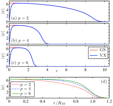
Figure 1: (Color online) Radial profile $|\psi|$ as a function of $r$ for the ground state (GS, red dashed line) and the vortex state (VX, blue solid line) inside the trapping potential $V(r)=\frac{1}{p}r^{p}$ with $\mu=40$ for (a) $p=2$, (b) $p=4$, and (c) $p=6$. Note that in the Thomas-Fermi limit, the size of the vortices for the different potentials is essentially the same. This property, determined by the healing length, is controlled by the chemical potential $\mu$ which is constant ($\mu=40$) for the three cases. Panel (d) depicts the GS profiles as a function of the rescaled distance $r/R_{\rm TF}$ where the corresponding TF radii are given by $R_{\rm TF}=(p\mu)^{1/p}$.

It is important to stress that the logarithmic term in the energy, and hence in the precession frequency, is always present independently of the chosen power $p$ of the confining potential. This logarithmic term is crucial (dominant) for parabolic trapping potentials (see Eq. (6) and Refs. svidz ; Fetter_review_2009 ). However, as shown above, for potentials with powers larger than quadratic, the logarithmic term decays faster than the remaining terms in the asymptotic expression near the origin, and hence it is no longer dominating the relevant asymptotics. Nonetheless, it should be pointed out that far from the origin, the logarithmic correction terms will indeed become significant and the full expression without discarding these terms needs to be used.

In order to complement the above result for the precession frequency using the asymptotics for the energy, we have also employed a direct matching asymptotics analysis on Eq. (1) that yields precisely the same asymptotic result as in Eq. (9). Details on this matched asymptotic procedure can be found in Appendix B. We now turn to a numerical examination of the relevant findings.

III Numerical Results

In our numerical work, we study $V=\frac{1}{p}r^{p}$, where $p=2,4$ and 6. We start by showing the ground and vortex states at a typical (relatively large) value of the chemical potential, $\mu=40$, within the so-called Thomas-Fermi regime. In this regime, the radial background density (i.e., the density of the ground state) can be well approximated as $|\psi|^{2}\approx|\psi_{\rm TF}|^{2}=\mu-V(r)$. Relevant results as depicted in Fig. 1. One can observe that the states near $r=0$ are almost identical for different potentials. In particular, the density of the ground states at $r=0$ and the width of the vortices is essentially dominated by the chemical potential which controls the corresponding healing length. The size of the states gets smaller as $p$ increases or, equivalently, as the atoms are bound tighter.

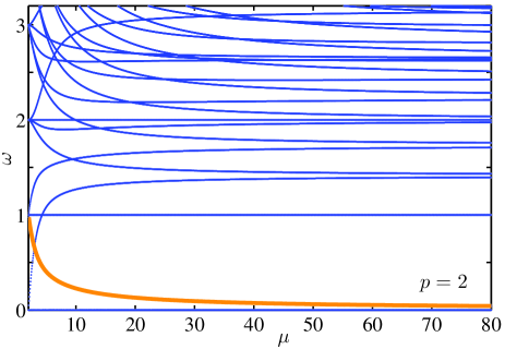
Figure 2: (Color online) The BdG spectrum for the vortex in the quadratic potential. The lowest mode, highlighted in orange, is the one of interest as it corresponds to the vortex precession around the trap center.

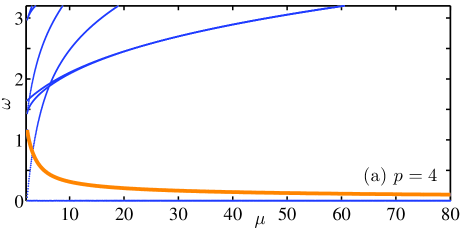
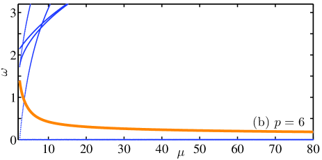
Figure 3: (Color online) The vortex spectrum in the (a) quartic and (b) sextic potentials. The lowest mode which is highlighted in orange similar to the quadratic potential is the vortex precession mode around the trap center.

Let us start by showing the numerical results for the parabolic potential $V(r)=\frac{1}{2}r^{2}$ (i.e., $\Omega=1$). The Bogolyubov-de Gennes (BdG) stability spectrum for the steady state consisting of a unit-charge vortex at the center of the trap is depicted in Fig. 2. Among all the modes in the spectrum, the lowest is the one that is not found in the spectrum of linearization around the ground state. Instead, when we excite this mode, we find that it leads the vortex to a precessional motion around the center of the trap; thus, the frequency of this mode corresponds to the frequency of the associated precession middel . This precessional mode is depicted with a orange line in Fig. 2.

We now go beyond the well-known parabolic case, in order to examine other case examples that the general theory can tackle. More specifically, we consider the quartic case of $p=4$ and the sextic case of $p=6$. The BdG spectra for the corresponding steady state vortex configurations are shown in Fig. 3. Note that both potentials still have the vortex precession mode (see eigenfrequency mode depicted in orange), because of the symmetry of the potential. Indeed, we find that in both cases it remains the only mode asymptoting to $\omega=0$, as the chemical potential $\mu$ is increased. The case examples of the associated dynamics that we have chosen to show are for $\mu=40$. This is much larger than that of the case $p=2$, because the cases $p=4$ and $p=6$ involve a tighter binding trap. It is interesting to note that the vortex in all three cases is remarkably stable for all the values of the chemical potential that we have examined.

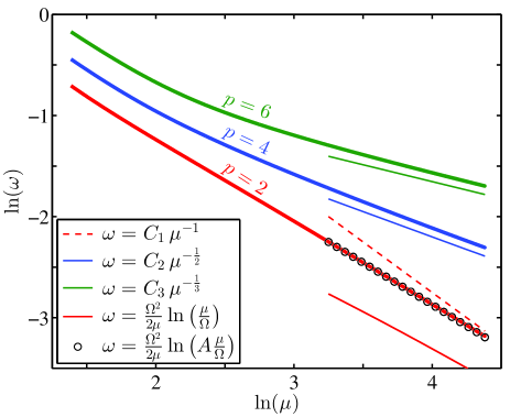
Figure 4: (Color online) Scaling of the precession frequency $\omega$ on the chemical potential $\mu$. The thick lines corresponds to the precession frequency extracted from the numerically obtained spectra and the asymptotic approximations are depicted with thin lines ($C_{i}$ are arbitrary constants chosen for ease of exposition). The case of $p=2$ decays slower compared with the power scaling (see thin red dashed line) due to the logarithmic correction, while for $p=4$ and $p=6$, the predictions and the spectrum appears to compare well with each other, suggesting a good agreement with the analytical prediction of Eq. (9). The black circles correspond to a correction to the asymptotic formula (6), namely Eq. (10) with $A=8.88$, see Ref. middel .

Let us now focus on the scaling of the precession frequency $\omega$ (close to the center of the trap) on the chemical potential for all three cases of $p=2$, $4$ and $6$. The corresponding results are depicted in Fig. 4 and are compared to our theoretical prediction, as encapsulated in Eq. (9) . In this figure, the relevance of our analytical prediction, and especially of the corresponding scaling is evident. Indeed, once the (small and) intermediate chemical potential regime (where all potentials scale similarly) is bypassed and the large chemical potential TF regime is reached, the different potentials scale differently. More specifically, it is found that the scaling prediction of Eq. (9) is closely followed by the spectral numerical results for $p=4$ and $p=6$ (see, respectively, the thin solid blue and green lines). On the other hand, for $p=2$, the prediction of Eq. (9) (see red dashed line) is incorrect as the dominant term in this case has a logarithmic form, see Eq. (6) and the thin solid red line in Fig. 4. It is worth mentioning that, although the precession frequency predicted by Eq. (6) has the correct scaling, a numerical factor has been used in order to incorporate the sub-dominant contributions to the frequency scaling according to $\mu^{-1}$ middel in a quantitative fashion. This is depicted by the black circles in the figure corresponding to

$$\omega=\frac{\Omega^{2}}{2\mu}\ln\left(A\frac{\mu}{\Omega}\right),$$ (10)

with the numerical factor $A=8.88$, see Ref. middel .

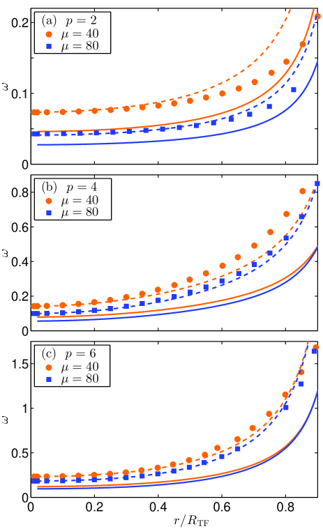
Figure 5: (Color online) Scaling of the precession frequency as a function of the rescaled vortex position for the different potentials $V(r)=\frac{1}{p}r^{p}$ with $\mu=40$ and $\mu=80$. A vortex is displaced from $r=0$ and its precession frequency is extracted from its dynamical evolution (see text) and depicted with orange (blue) circles (squares) for $\mu=40$ ($\mu=80$). The solid lines depict the theoretical predictions from evaluating Eq. (5) and using the limit $\xi\ll r$. The dashed curves for the $p=2$ case correspond to the corrected precession of Eq. (10) while the dashed curves for the $p=4$ and $p=6$ cases depict the rescaled theoretical predictions so as to match the precession frequency in the limit $r=0$. These rescaling coefficients correspond to, respectively for $\mu=40$ and $\mu=80$, $p=4$: 1.7944 and 1.7804, and $p=6$: 1.9302 and 1.9114.

To complement the description for the vortex precession around the center of the trap, we also measure the dependence of this frequency as the vortex is shifted away from $r=0$. In practice, a straightforward way to observe this precession, involves shifting the vortex off of its equilibrium position at $r=0$ and then following its circular motion around the center. Figure 5 depicts the departure of the precession frequency from the corresponding eigenfrequency, $\omega_{0}$, at $r=0$ measured from the center of the trap. The figure also depicts the analytical prediction given from evaluating Eq. (5) and using the limit $\xi\ll r$ (see solid curves in the figure). It is evident from these results that the theory underestimates the precession frequency. We attribute this discrepancy to two possible factors:

• The ansatz used in the theory completely disregards the internal spatial structure of the vortex as it effectively treats it as a point vortex, an approximation valid as $\mu\rightarrow\infty$. For instance, optimizing the vortex width appears to be an important factor in the success of more refined (yet less straightforwardly tractable in the general case) variational approaches such as that of Ref. castin .

• Secondly, when estimating the precession frequency at the center of the trap ($r=0$) the limit $0<\xi\ll r$ is obviously violated as the healing length $\xi$ is finite.

Although the theoretical results fail to precisely predict the precession frequency at $r=0$, they are able to give the right tendency for the departure of the precession frequency as the vortex is displaced away from the origin. In fact, after applying suitable modifications (see dashed curves in Fig. 5), the predictions produce a good quantitative match for the departure of the precession frequency from $\omega_{0}$ as $r$ departs from $r=0$ (especially for small and intermediate values of $r$ and progressively better for larger values of $\mu$, in line with the underlying premise of the theory). Specifically, in the $p=2$ case, where the dominant term on the precession as a function of $r$ is logarithmic, we employ the correction given in Eq. (10) Ref. middel . On the other hand, for the $p=4$ and $p=6$ cases, the dominant terms are algebraic and thus we opt for a multiplicative rescaling factor chosen so as to match the precession frequency at the origin (see Fig. 5).

IV Conclusions and Future Challenges

In the present work, we have explored the motion of vortices in general radially symmetric potentials. We have found that similarly to the well known parabolic case, the motion of the vortices involves a precession. The main result of the present work concerns the vortex precession frequency and its dependence on both the chemical potential of the background cloud and the location of the vortex within the condensate. Utilizing a variational formulation generalizing the work of Ref. svidz , we were able to provide closed form expressions for the precession frequency relevant in the large chemical potential limit (Thomas-Fermi regime). These expressions permitted us to appreciate the power law scaling of the precession frequency on the chemical potential and how the relevant dependence becomes slower as $p$ increases. The limitations of the theory in identifying the precession mode frequency at the origin were explained and it was shown how a suitable amendment can be used to capture its dependence on the radial position of an off-center vortex.

While in the present work we have explored the general (radial) potential motion of a single vortex, numerous related questions naturally emerge from this study. Here, we considered isotropic potentials which still constitute a subject of active investigation Esposito and some controversy regarding the physical interpretation of the origin of the vortex motion simula . Yet, anisotropic potentials are also quite relevant in atomic BECs svidz ; siambook . Examining vortex motion in such anisotropic settings under general $V$ would be certainly of interest. Furthermore, combining an understanding of the single vortex motion in a general potential with that of the inter-vortex interaction will enable identifying multi-vortex (cluster and crystal) states for arbitrary trapped BEC systems. Another possibility for future research could be to consider pseudo-potentials stemming from considering space (radial) dependent nonlinearities Boris_pseudo_potential with different power law prescriptions.

Finally, while the above ideas are natural to be first developed in two-dimensional settings, generalizing them to vortex rings in three-dimensional frameworks komineas would also be of interest in its own right. Some of these directions are currently under consideration and will be reported in future publications.

Appendix A Energy calculation

As explained in Ref. kimfetter , the principal contribution to the energy stems from the gradient term, which upon our ansatz (3) and in the TF approximation can be written as:

$$E=\frac{\mu}{2}\int_{0}^{R_{\rm TF}}rdr\int_{0}^{2\pi}d\theta\left(1-\frac{V(r)}{\mu}\right)\frac{1}{r^{2}+r_{1}^{2}-2rr_{1}\cos(\theta-\phi_{1})},$$

where, again, $(r1,\phi_{1})$ is the vortex position in polar coordinates. This integral can be split into two radial contributions namely the integral $I_{1}$ from $0$ to $r_{1}-\xi$ and $I_{2}$ from $r_{1}+\xi$ to $R_{\rm TF}$. This way, using the characteristic length of the vortex core, namely the healing length $\xi$, we regularize the integral. These two integrals can then be rewritten as:

$$I_{1} = \frac{1}{2}\int_{0}^{r_{1}-\xi}dr\int_{0}^{2\pi}d\theta\,\frac{r(\mu-V(r))}{r_{1}^{2}-r^{2}}\left(1+2\sum_{n}\left(\frac{r}{r_{1}}\right)^{n}\cos(n(\theta-\phi_{1}))\right),$$

$$I_{2} = \frac{1}{2}\int_{r_{1}+\xi}^{R_{\rm TF}}dr\int_{0}^{2\pi}d\theta\,\frac{r(\mu-V(r))}{r^{2}-r_{1}^{2}}\left(1+2\sum_{n}\left(\frac{r_{1}}{r}\right)^{n}\cos(n(\theta-\phi_{1}))\right),$$

which finally yield the following resulting expressions used in Eq. (LABEL:poten):

$$I_{1} = \pi\int_{0}^{r_{1}-\xi}dr\frac{r(\mu-V(r))}{r_{1}^{2}-r^{2}},$$

$$I_{2} = \pi\int_{r_{1}+\xi}^{R_{\rm TF}}dr\frac{r(\mu-V(r))}{r^{2}-r_{1}^{2}}.$$

Appendix B Matched asymptotics calculation

We hereby obtain an alternative derivation for the precession frequency of Eq. (9) using matched asymptotics directly on the original model (1). We seek for stationary solutions to Eq. (1) of the form $\psi=\psi^{(0)}e^{-i\mu t}$ satisfying the steady state Eq. (2). By scaling variables using $\tilde{x}={x}/R_{\rm TF}$, $\tilde{y}={y}/R_{\rm TF}$, $\tilde{\psi}={\psi^{(0)}}/\sqrt{\mu}$, and $\tilde{t}={t}/(2R_{\rm TF}^{2})$, we obtain:

$$-i\psi_{t}=\Delta\psi+\frac{1}{\varepsilon^{2}}\left(1-V(r)-|\psi|^{2}\right)\psi,$$

with $\varepsilon^{2}={1}/(2R_{\rm TF}^{2}\mu)$ and where, for ease of exposition, we have dropped tildes and superscripts. Note that the core size of the vortex is of order $\varepsilon$.

Away from the core of the vortex, to leading order in $\varepsilon$, we have $1-V(\vec{r})-|\psi(\vec{r})|^{2}=0$, which suggests the separation

$$\psi=\psi_{\rm TF}\,e^{iS}$$

where $\psi_{\rm TF}=\sqrt{1-V(\vec{r})}$ is the TF approximation and $S$ satisfies:

$$\psi_{\rm TF}\Delta S+2\nabla\psi_{\rm TF}\cdot\nabla S=0,$$

$$\nabla\times\nabla S=2\pi\delta(\vec{r}-\vec{r}_{1}),$$

where $\delta$ is the Dirac-delta function centered at the vortex location $\vec{r}_{1}$. By examining the local behavior of $S$, we can obtain:

$$\psi(\vec{r})\sim\left(\psi_{\rm TF}(\vec{r}_{1})+\nabla\psi_{\rm TF}(\vec{r}_{1}){\cdot(r-\vec{r}_{1})}\right){e^{i\varphi}}\left(1+i\ln|\vec{r}-\vec{r}_{1}|{\frac{\nabla^{\bot}\psi_{\rm TF}(\vec{r}_{1})}{\psi_{\rm TF}(\vec{r}_{1})}}\cdot(\vec{r}-\vec{r}_{1})+\vec{K}\cdot(\vec{r}-\vec{r}_{1})\right),~{}~{}{\rm as}~{}~{}\vec{r}\rightarrow\vec{r}_{1},$$ (11)

where $\vec{K}\equiv\lim_{\vec{r}\rightarrow\vec{r}_{1}}\nabla\left(S-{\varphi}\right)$, $\varphi={\rm ang}(\vec{r}-\vec{r}_{1})$, and the operator $(\cdot)^{\bot}$ is defined, in Cartesian coordinates, by $(a,b)^{\bot}\equiv(-b,a)$.

Near the core of the vortex, we denote the stretched variable $\vec{\rho}=(\vec{r}-\vec{r}_{1}(t))/{\varepsilon}$ and look for the solution in the form:

$$\psi=\psi_{0}({\vec{\rho}})+\varepsilon\psi_{1}({\vec{\rho}})+\cdots$$

Matching the first two orders of $\varepsilon$ yields:

$$0 = \Delta_{{\vec{\rho}}}\psi_{0}+(1-V(|\vec{r_{1}}|))\psi_{0}-|\psi_{0}|^{2}\psi_{0}$$

$${i\,\dot{\vec{r}}_{1}}\cdot\nabla_{{\vec{\rho}}}\psi_{0}{+\nabla V(\vec{r}_{1})}\cdot{\vec{\rho}}\psi_{0} = \Delta_{{\vec{\rho}}}\psi_{1}+{(1-V(|\vec{r}_{1})|)}\psi_{1}-|\psi_{0}|^{2}\psi_{1}-\psi_{0}\left(\psi_{0}\psi^{*}_{1}+\psi_{1}\psi^{*}_{0}\right),$$

where the overdot denotes time derivative. Now, in order to match with the outer region, we only need the asymptotic behavior of the inner solution as $|{\vec{\rho}}|\rightarrow\infty$. A detailed analysis for this asymptotics yields Shuangquan_preprint

$$\psi_{0} \rightarrow\psi_{\rm TF}e^{i{\theta}}, ~{}~{}{\rm as}~{}~{}|{\vec{\rho}}|\rightarrow\infty,$$

$$\psi_{1} \rightarrow\left(\nabla\psi_{\rm TF}(\vec{r}_{1})\cdot{\vec{\rho}}+{i}\ln(\psi_{\rm TF}|{\vec{\rho}}|)\nabla^{\bot}\psi_{\rm TF}\cdot{\vec{\rho}}{+}\frac{1}{2}\psi_{\rm TF}(\vec{r}_{1})\dot{\vec{r}}_{1}\cdot{\vec{\rho}}\right)e^{i{\theta}}, ~{}~{}{\rm as}~{}~{}|{\vec{\rho}}|\rightarrow\infty,$$

and therefore

$$\psi=\psi_{\rm TF}(\vec{r}_{1})e^{i{\theta}}+\varepsilon\left(\nabla\psi_{\rm TF}(\vec{r}_{1})\cdot{\vec{\rho}}+{i}\ln(\psi_{\rm TF}|{\vec{\rho}}|)\nabla^{\bot}\psi_{\rm TF}(\vec{r}_{1})\cdot{\vec{\rho}}{+}\frac{1}{2}\psi_{\rm TF}(\vec{r}_{1})\dot{\vec{r}}_{1}\cdot{\vec{\rho}}\right)e^{i{\theta}},~{}~{}{\rm as}~{}~{}|{\vec{\rho}}|\rightarrow\infty.$$ (12)

Employing asymptotic matching between Eqs. (11) and (12), recalling that $\vec{\rho}=(\vec{r}-\vec{r}_{1}(t))/{\varepsilon}$, yields:

$$\frac{-2\vec{K}{+}\dot{\vec{r}}_{1}}{\ln\varepsilon-\ln(\psi_{\rm TF}(\vec{r}_{1}))}-\frac{2\nabla^{\bot}\psi_{\rm TF}(\vec{r}_{1})}{\psi_{\rm TF}(\vec{r}_{1})}=0.$$

Thus, to leading order of $\nu\equiv{-1}/{\ln\varepsilon}$, we obtain

$$\dot{\vec{r}}_{1}={-}\frac{2}{\nu}\frac{\nabla^{\bot}\psi_{\rm TF}(\vec{r}_{1})}{\psi_{\rm TF}(\vec{r}_{1})}{+}2\vec{K}.$$ (13)

Now, depending on the range of $|\vec{r}_{1}|$, we have two different leading order dynamics:

• If $|\nabla^{\bot}\psi_{\rm TF}(\vec{r}_{1})|\ll\nu$: the dominant term in (13) is $\vec{K}$ and thus

  $$\dot{\vec{r}}_{1}={2\vec{K}}$$ (14)

• If $|\nabla^{\bot}\psi_{\rm TF}(\vec{r}_{1})|\gg\nu$: the dominant term in (13) is the first term and thus

  $$\dot{\vec{r}}_{1}={-}\frac{2}{\nu}\frac{\nabla^{\bot}\psi_{\rm TF}(\vec{r}_{1})}{\psi_{\rm TF}(\vec{r}_{1})}$$ (15)

While the comparison of the relevant cases in terms of the dominant mathematical contribution is straightforward, assigning an intuitive explanation to these different scenarios is an open topic worthwhile of further consideration in future studies. By returning to the original (unscaled) variable $t$, Eq. (14) finally yields the following expression for the rate of change of the vortex position vector $\vec{r}_{1}$:

$$\dot{\vec{r}}_{1}=\frac{\vec{K}}{R_{\rm TF}^{2}},$$

which, by noting that $\vec{K}$ is an azimuthal vector, is in agreement with the precession frequency that was obtained using the asymptotic expansion for the energy in Sec. II.5:

$$\omega\sim\frac{1}{R_{\rm TF}^{2}}.$$ (16)

References

- (1) C. J. Pethick and H. Smith, Bose-Einstein condensation in dilute gases (Cambridge University Press, Cambridge, 2002).
- (2) L. P. Pitaevskii and S. Stringari, Bose-Einstein Condensation, Oxford University Press (Oxford, 2003).
- (3) P. G. Kevrekidis, D. J. Frantzeskakis, and R. Carretero-González, The Defocusing Nonlinear Schrödinger Equation, SIAM (Philadelphia, 2015).
- (4) B. P. Anderson, P. C. Haljan, C. E. Wieman, and E. A. Cornell, Phys. Rev. Lett. 85, 2857 (2000).
- (5) P. C. Haljan, B. P. Anderson, I. Coddington, and E. A. Cornell, Phys. Rev. Lett. 86, 2922 (2001).
- (6) V. Bretin, P. Rosenbusch, F. Chevy, G. V. Shlyapnikov, and J. Dalibard, Phys. Rev. Lett. 90, 100403 (2003).
- (7) T. W. Neely, E. C. Samson, A. S. Bradley, M. J. Davis, and B. P. Anderson, Phys. Rev. Lett. 104, 160401 (2010).
- (8) D. V. Freilich, D. M. Bianchi, A. M. Kaufman, T. K. Langin, and D. S. Hall, Real-Time Dynamics of Single Vortex Lines and Vortex Dipoles in a Bose-Einstein Condensate, Science 329, 1182–1185 (2010).
- (9) S. Middelkamp, P. J. Torres, P. G. Kevrekidis, D. J. Frantzeskakis, R. Carretero-González, P. Schmelcher, D. V. Freilich, and D. S. Hall, Phys. Rev. A 84, 011605(R) (2011).
- (10) R. Navarro, R. Carretero-González, P. J. Torres, P. G. Kevrekidis, D. J. Frantzeskakis, M. W. Ray, E. Altuntaş, and D. S. Hall, Phys. Rev. Lett. 110, 225301 (2013).
- (11) Y. Shin, M. Saba, M. Vengalattore, T. A. Pasquini, C. Sanner, A. E. Leanhardt, M. Prentiss, D. E. Pritchard, and W. Ketterle, Dynamical Instability of a Doubly Quantized Vortex in a Bose-Einstein Condensate, Phys. Rev. Lett. 93, 160406 (2004).
- (12) T. Isoshima, M. Okano, H. Yasuda, K. Kasa, J. A. M. Huhtamäki, M. Kumakura, and Y. Takahashi, Phys. Rev. Lett. 99, 200403 (2007).
- (13) B. P. Anderson, P. C. Haljan, C. A. Regal, D. L. Feder, L. A. Collins, C. W. Clark, and E. A. Cornell, Phys. Rev. Lett. 86, 2926 (2001).
- (14) Z. Dutton, M. Budde, C. Slowe, and L. V. Hau, Science 293, 663 (2001).
- (15) M. J. H. Ku, B. Mukherjee, T. Yefsah, and M. W. Zwierlein, arXiv:1507.01047.
- (16) P. Engels, I. Coddington, P. C. Haljan, and E. A. Cornell, Phys. Rev. Lett. 89, 100403 (2002).
- (17) I. Coddington, P. Engels, V. Schweikhard, and E. A. Cornell, Phys. Rev. Lett. 91, 100402 (2003).
- (18) N. L. Smith, W. H. Heathcote, J. M. Krueger, and C. J. Foot, Phys. Rev. Lett. 93, 080406 (2004).
- (19) V. Schweikhard, I. Coddington, P. Engels, S. Tung, and E. A. Cornell, Phys. Rev. Lett. 93, 210403 (2004).
- (20) S. Tung, V. Schweikhard, and E. A. Cornell, Phys. Rev. Lett. 97, 240402 (2006).
- (21) E. A. L. Henn, J. A. Seman, G. Roati, K. M. F. Magalhães, and V. S. Bagnato, Phys. Rev. Lett. 103, 045301 (2009).
- (22) T. W. Neely, A. S. Bradley, E. C. Samson, S. J. Rooney, E. M. Wright, K. J. H. Law, R. Carretero-González, P. G. Kevrekidis, M. J. Davis, and B. P. Anderson, Phys. Rev. Lett. 111, 235301 (2013).
- (23) W. J. Kwon, G. Moon, J.-Y. Choi, S. W. Seo, and Y.-I. Shin, Phys. Rev. A 90, 063627 (2014).
- (24) J.-Y. Choi, S. W. Seo, and Y.-i. Shin, Phys. Rev. Lett. 110, 175302 (2013)
- (25) G. Moon, W. J. Kwon, H. Lee, and Y.-i. Shin Phys. Rev. A 92, 051601(R) (2015).
- (26) K. Henderson, C. Ryu, C. MacCormick, and M. G. Boshier, New J. Phys. 11, 043030 (2009).
- (27) S. E. Pollack, D. Dries, M. Junker, Y. P. Chen, T. A. Corcovilos, and R. G. Hulet, Phys. Rev. Lett. 102, 090402 (2009).
- (28) J. H. V. Nguyen, D. Luo, and R. G. Hulet, Science 356, 422 (2017).
- (29) A. Ramanathan, K. C. Wright, S. R. Muniz, M. Zelan, W. T. Hill, C. J. Lobb, K. Helmerson, W. D. Phillips, and G. K. Campbell, Phys. Rev. Lett. 106, 130401 (2011); K. C. Wright, R. B. Blakestad, C. J. Lobb, W. D. Phillips, and G. K. Campbell, Phys. Rev. Lett. 110 025302 (2013);
- (30) C. Ryu, K. C. Henderson, and M.G. Boshier, New J. Phys. 16, 013046 (2014).
- (31) J.K. Kim and A.L. Fetter, Phys. Rev. A 70, 043624 (2004).
- (32) E. Lundh and P. Ao, Phys. Rev. A 61, 063612 (2000).
- (33) A. L. Fetter and A. A. Svidzinsky, J. of Phys.: Condensed Matter 13, R135 (2001).
- (34) S. Middelkamp, P. G. Kevrekidis, D. J. Frantzeskakis, R. Carretero-González, and P. Schmelcher, Phys. Rev. A 82, 013646 (2010).
- (35) D. E. Pelinovsky and P. G. Kevrekidis, Nonlinearity 24, 1271 (2011).
- (36) Y. Castin and R. Dum, Eur. Phys. J. D 7, 399 (1999).
- (37) A. L. Fetter, Rev. Mod. Phys. 81 (2009) 647.
- (38) W. Wang, P. G. Kevrekidis, R. Carretero-González, and D. J. Frantzeskakis, Phys. Rev. A 93, 023630 (2016); W. Wang and P. G. Kevrekidis, Phys. Rev. E 95, 032201 (2017).
- (39) A. Esposito, R. Krichevsky, and A. Nicolis, Phys. Rev. A 96 033615 (2017).
- (40) A.J. Groszek, D.M. Paganin, K. Helmerson, T.P. Simula, arxiv:1708.09202.
- (41) Y. V. Kartashov, B. A. Malomed, V. A. Vysloukh, M. R. Belić, and L. Torner, Opt. Lett. 42 (2017) 446–449.
- (42) S. Komineas, Eur. Phys. J. Spec. Topics, 147, 133 (2007).
- (43) Shuangquan Xie, T. Kolokolnikov, and P. G. Kevrekidis, arXiv:1708.04336.