“Parallel Training Considered Harmful?”:
Comparing series-parallel and parallel feedforward network training

Abstract

Neural network models for dynamic systems can be trained either in parallel or in series-parallel configurations. Influenced by early arguments, several papers justify the choice of series-parallel rather than parallel configuration claiming it has a lower computational cost, better stability properties during training and provides more accurate results. Other published results, on the other hand, defend parallel training as being more robust and capable of yielding more accurate long-term predictions. The main contribution of this paper is to present a study comparing both methods under the same unified framework with special attention to three aspects: i) robustness of the estimation in the presence of noise; ii) computational cost; and, iii) convergence. A unifying mathematical framework and simulation studies show situations where each training method provides superior validation results and suggest that parallel training is generally better in more realistic scenarios. An example using measured data seems to reinforce such a claim. Complexity analysis and numerical examples show that both methods have similar computational cost although series-parallel training is more amenable to parallelization. Some informal discussion about stability and convergence properties is presented and explored in the examples.

url]antonior92.github.io

1 Introduction

Neural networks are widely used and studied for modeling nonlinear dynamic systems [1, 2]. In the seminal paper by Narenda and Parthasarathy [1] series-parallel and parallel configurations were introduced as possible architectures for training neural networks with data from dynamic systems. In both cases the neural network parameters are estimated by minimizing the error between predicted and measured values. When training the neural network in series-parallel configuration measured  values from past instants are used to make one-step-ahead predictions. On the other hand, when training in parallel configuration previously predicted  outputs are fed back into the network to compute what is known as the free-run simulation of the network.

In a very influential paper [1], training in series-parallel configuration is said to be preferable to parallel configuration for three main reasons: (i) all signals generated in the identification procedure for series-parallel configuration are bounded, while this is not guaranteed for the parallel configuration (this argument is also mentioned in [3, 4]); (ii) for the parallel configuration a modified version of backpropagation is needed, resulting in a greater computational cost for training, while the standard backpropagation can be used in the context of the series-parallel configuration (this has also been mentioned in [5, 6, 7]); and, (iii) assuming that the error tends asymptotically to small values, the simulated output is not so different from the actual one and, therefore, the results obtained from two configurations would not be significantly different (this reasoning was repeated in [8, 9, 10]). An additional reason that also appears sometimes in the literature is that: (iv) the series-parallel training provides better results because of more accurate inputs to the neural network during training (this argument has also been used in [6, 7, 11, 12, 13, 14]).

It is clear that the seminal paper [1] still has great influence on the literature. However, a number of subtle aspects related to the alleged reasons for preferring series-parallel training were not discussed in that paper and, from the literature, seem to remain unnoticed in general. This may have important practical consequences especially in situations where parallel training would be the best option. Hence, one of the aims of this work is to establish the validity of such arguments.

Other papers followed as somewhat complimentary track highlighting the strengths of parallel training in system identification. For instance, according to [15, 16] neural networks trained in parallel yield more accurate long-term predictions than the ones trained in series-parallel; it has been shown that for diverse types of models, including neural networks, parallel training can be more robust than series-parallel training in the presence of some types of noise [17]; and, in a series of papers Piroddi and co-workers have argued that parallel-training (i.e. free-run simulation error minimization) is a promising technique for structure selection of polynomial models [18, 19, 20, 21, 22]. Some papers also compare the two training methods in practical settings: in [23] neural network parallel models present better validation results than series-parallel models for modeling a boiler unit; and, in [24] parallel training provided the best results when estimating the parameters of a battery.

The main contribution of this paper is to provide a detailed comparison of parallel and series-parallel training. Three aspects receive special attention: (i) computational cost; (ii) robustness of the estimation in the presence of noise; and, (iii) convergence. The rest of the paper is organized as follows: Section 2 reviews backpropagation and nonlinear least-squares algorithms. Section 3 provides the nonlinear least-squares framework used along this paper. A complexity analysis is presented in Section 4. Section 5 give asymptotic properties of the methods in the presence noise. In Section 6, examples are used to investigate the effect of the noise and the training time. Section 7 discusses signal unboundedness, the convergence to “poor” local solutions and computational considerations. Final comments and future work are presented in Section 8.

2 Background

This section provides a quick review of algorithms and ideas used to build our formulation: Section 2.1 explains series-parallel and parallel training; Section 2.2 explains the Levenberg-Marquardt algorithm [25], presenting a formulation similar to the one in [26]; Section 2.3 explains a modified backpropagation algorithm, proposed in [27].

2.1 Parallel vs series-parallel training

Figure 1 illustrates the difference between parallel and series-parallel training. Parallel configuration feeds the output back to the input of the network and, hence, uses its own previous values to predict the next output of the system being modeled. Series-parallel configuration, on the other hand, uses the true measured output rather than feeding back the estimated one. We formalize these concepts along this section.

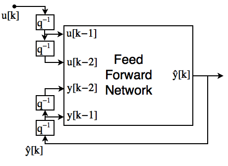
(a) Parallel

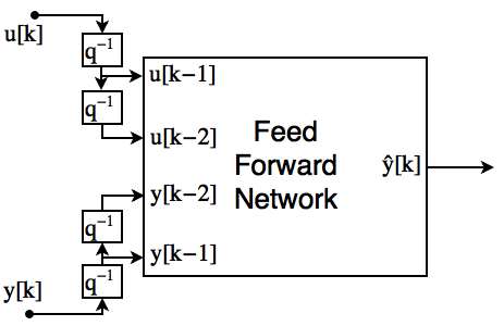
(b) Series-parallel

Figure 1: Parallel and series-parallel neural network architectures for modeling the dynamic system $\mathbf{y}[k]=\mathbf{F}(\mathbf{y}[k-1],\mathbf{y}[k-2],\mathbf{u}[k-1],\mathbf{u}[k-2])$. The delay operator $q^{-1}$ is such that $\mathbf{y}[k-1]=q^{-1}\mathbf{y}[k]$.

Consider the following dataset: $\mathcal{Z}=\{(\mathbf{u}[k],\mathbf{y}[k]),k=1,2,\ldots,N\},$ containing a sequence of sampled inputs-output pairs. Here ${\mathbf{u}[k]\in\mathbb{R}^{N_{u}}}$ and ${\mathbf{y}[k]\in\mathbb{R}^{N_{y}}}$ are vectors containing all the inputs and outputs of interest at instant $k$. The output $\mathbf{y}[k]$ is correlated with its own past values $\mathbf{y}[k-1]$, $\mathbf{y}[k-2]$, $\mathbf{y}[k-3]$, $\cdots$, and with past input values $\mathbf{u}[k-\tau_{d}]$, $\mathbf{u}[k-\tau_{d}-1]$, $\mathbf{u}[k-\tau_{d}-2]$, $\cdots$. The integer $\tau_{d}\geq 0$ is the input-output delay (when changes in the input take some time to affect the output).

The aim is to find a difference equation model:

$$\mathbf{y}[k]=\mathbf{F}(\mathbf{y}[k-1],\ldots,\mathbf{y}[k-n_{y}],\mathbf{u}[k-\tau_{d}],\ldots,\mathbf{u}[k-n_{u}];\mathbf{\Theta}),$$ (1)

that best describes the data in $\mathcal{Z}$. The model is described by the nonlinear function $\mathbf{F}$ parameterized by ${\mathbf{\Theta}\in\mathbb{R}^{N_{\Theta}}}$; the maximum input and output lags $n_{y}$ and $n_{u}$; and, the input-output delay $\tau_{d}$. It is assumed that a finite number of past terms can be used to describe the output.

Neural networks are an appropriate choice for representing the function $\mathbf{F}$ because they are universal approximators. A neural network with as few as one hidden layer can approximate any measurable function $\mathbf{F}^{*}$ with arbitrary accuracy within a given compact set [28].

From now on, the simplified notation: ${\footnotesize\underline{\mathbf{y}}_{[k]}=[\mathbf{y}[k-1]^{T},\ldots,\mathbf{y}[k-n_{y}]^{T}]^{T}}$,
${\footnotesize\underline{\mathbf{u}}_{[k]}=[\mathbf{u}[k-\tau_{d}]^{T},\ldots,\mathbf{u}[k-n_{u}]^{T}]^{T}}$ will be used, hence, Equation (1) can be rewritten as: $\mathbf{y}[k]=\mathbf{F}(\underline{\mathbf{y}}_{[k]},\underline{\mathbf{u}}_{[k]};\mathbf{\Theta})$.

Definition 1 (One-step-ahead prediction).

For a given function $\mathbf{F}$, parameter vector $\mathbf{\Theta}$ and dataset $\mathcal{Z}$, the one-step-ahead prediction is defined as:

$$\hat{\mathbf{y}}_{1}[k]=\mathbf{F}(\underline{\mathbf{y}}_{[k]},\underline{\mathbf{u}}_{[k]};\mathbf{\Theta}),$$ (2)

Definition 2 (Free-run simulation).

For a given function $\mathbf{F}$, parameter vector $\mathbf{\Theta}$, dataset $\mathcal{Z}$ and a set of initial conditions $\{\mathbf{y}_{0}[k]\}_{k=1}^{n_{y}}$, the free-run simulation is defined using the recursive formula:

$$\hat{\mathbf{y}}_{s}[k]=\begin{dcases}\mathbf{y}_{0}[k],~{}1\leq k\leq n_{y};\\ \mathbf{F}(\hat{\mathbf{y}}_{s}[k-1],\ldots,\hat{\mathbf{y}}_{s}[k-n_{y}],\underline{\mathbf{u}}_{[k]};\mathbf{\Theta}),~{}k>n_{y},\end{dcases}$$ (3)

The vector of initial conditions is defined as ${\underline{\mathbf{y}}_{0}=[\mathbf{y}_{0}[1]^{T}}$, ${\ldots,\mathbf{y}_{0}[n_{y}]^{T}]^{T}}$.

Both training procedures minimize some norm of the error and may be regarded as prediction error methods. That is, let ${\mathbf{e}=[\mathbf{e}[1]^{T},\ldots,\mathbf{e}[N]^{T}]^{T}}$, in this paper we consider the parameters are estimated minimizing the sum of square errors $\tfrac{1}{2}\|\mathbf{\mathbf{e}}\|^{2}$. The one-step-ahead error, ${\mathbf{e}_{1}[k]={\hat{\mathbf{y}}_{1}[k]-\mathbf{y}[k]}}$, is used for series-parallel training and the free-run simulation error, ${\mathbf{e}_{s}[k]=\hat{\mathbf{y}}_{s}[k]-\mathbf{y}[k]}$, for parallel training.

2.2 Nonlinear least-squares

Let $\mathbf{\Theta}\in\mathbb{R}^{N_{\Theta}}$ be a vector of parameters and $\mathbf{e}(\mathbf{\Theta})\in\mathbb{R}^{N_{e}}$ an error vector. In order to estimate the parameter vector $\mathbf{\Theta}$ the sum of square errors $V(\mathbf{\Theta})=\tfrac{1}{2}\|\mathbf{e}(\mathbf{\Theta})\|^{2}$ is minimized. Its gradient vector and Hessian matrix may be computed as: [30, p. 246]

$$\tfrac{\partial V}{\partial\mathbf{\Theta}} = \left[\tfrac{\partial\mathbf{e}}{\partial\mathbf{\Theta}}\right]^{T}\mathbf{e}(\mathbf{\Theta}),$$ (4)

$$\tfrac{\partial^{2}V}{\partial\mathbf{\Theta}^{2}} = \left[\tfrac{\partial\mathbf{e}}{\partial\mathbf{\Theta}}\right]^{T}\left[\tfrac{\partial\mathbf{e}}{\partial\mathbf{\Theta}}\right]+\sum_{i=1}^{N_{e}}e_{i}\tfrac{\partial^{2}e_{i}}{\partial\mathbf{\Theta}^{2}},$$ (5)

where ${\tfrac{\partial\mathbf{e}}{\partial\mathbf{\Theta}}\in\mathbb{R}^{N_{e}\times N_{\Theta}}}$ is the Jacobian matrix associated with $\mathbf{e}(\mathbf{\Theta})$. Non-linear least-squares algorithms usually update the solution iteratively ($\mathbf{\Theta}^{n+1}=\mathbf{\Theta}^{n}+\Delta\mathbf{\Theta}^{n}$) and exploit the special structure of the gradient and Hessian of $V(\mathbf{\Theta})$, in order to compute the parameter update $\Delta\mathbf{\Theta}^{n}$.

The Levenberg-Marquardt algorithm considers a parameter update [25]:

$$\Delta\mathbf{\Theta}^{n}=-{\left[\left.\tfrac{\partial\mathbf{e}}{\partial\mathbf{\Theta}}\right|^{T}_{n}\left.\tfrac{\partial\mathbf{e}}{\partial\mathbf{\Theta}}\right|_{n}+\lambda^{n}D^{n}\right]}^{-1}\left[\left.\tfrac{\partial\mathbf{e}}{\partial\mathbf{\Theta}}\right|_{n}\right]^{T}\mathbf{e}_{n},$$ (6)

for which $\lambda^{n}$ is a non-negative scalar and $D^{n}$ is a non negative diagonal matrix. Furthermore, $\mathbf{e}_{n}$ and $\left.\tfrac{\partial\mathbf{e}}{\partial\mathbf{\Theta}}\right|_{n}$ are the error and the corresponding Jacobian matrix evaluated at $\mathbf{\Theta}^{n}$.

There are different ways of updating $\lambda^{n}$ and $D^{n}$. The update strategy presented here is similar to [26]. The elements of the diagonal matrix $D^{n}$ are chosen equal to the elements in the diagonal of $\left.\tfrac{\partial\mathbf{e}}{\partial\mathbf{\Theta}}\right|^{T}_{n}\left.\tfrac{\partial\mathbf{e}}{\partial\mathbf{\Theta}}\right|_{n}$. And $\lambda^{n}$ is increased or decreased according to the agreement between the local model $\left(\phi_{n}(\Delta\mathbf{\Theta}^{n})=\tfrac{1}{2}\left\|\mathbf{e}_{n}+\left[\left.\tfrac{\partial\mathbf{e}}{\partial\mathbf{\Theta}}\right|_{n}\right]\Delta\mathbf{\Theta}^{n}\right\|^{2}\right)$ and the real objective function $V(\mathbf{\Theta}_{n})$. The degree of agreement is measured using the following ratio:

$$\rho_{n}=\frac{V(\mathbf{\Theta}^{n})-V(\mathbf{\Theta}^{n}+\Delta\mathbf{\Theta}^{n})}{\phi_{n}(\mathbf{0})-\phi_{n}(\Delta\mathbf{\Theta}^{n})}.$$ (7)

One iteration of the algorithm is summarized next:

Algorithm 1 (Levenberg-Marquardt Iteration).

For a given $\mathbf{\Theta}^{n}$ and $\lambda^{n}$:

1. Compute $\mathbf{e}(\mathbf{\Theta}^{n})$ and $\tfrac{\partial\mathbf{e}}{\partial\mathbf{\Theta}}(\mathbf{\Theta}^{n})$, if not already computed.

2. $\text{diag}({D}^{n})\leftarrow\text{diag}\left(\left.\tfrac{\partial\mathbf{e}}{\partial\mathbf{\Theta}}\right|^{T}_{n}\left.\tfrac{\partial\mathbf{e}}{\partial\mathbf{\Theta}}\right|_{n}\right)$.

3. Solve (6) and compute $\Delta\mathbf{\Theta}^{n}$ .

4. Compute $\rho_{n}$ as in (7).

5. $\lambda^{n+1}\leftarrow 4\lambda^{n}$ if $\rho_{n}>\tfrac{3}{4}$; $\lambda^{n+1}\leftarrow\tfrac{1}{2}\lambda^{n}$ if $\rho_{n}<\tfrac{1}{4}$; otherwise, $\lambda^{n+1}\leftarrow\lambda^{n}$ .

6. $\mathbf{\Theta}^{n+1}\leftarrow\mathbf{\Theta}^{n}+\Delta\mathbf{\Theta}^{n}$ if $\rho_{n}>10^{-3}$; otherwise, $\mathbf{\Theta}^{n+1}\leftarrow\mathbf{\Theta}^{n}$.

7. $n=n+1$.

The backpropagation algorithm, which can be used for computing the derivative of static functions is explained in the sequence. How to adapt this algorithm in order to compute the Jacobian matrix both for parallel and series-parallel training is explained in Section 3.

2.3 Backpropagation

Consider a multi-layer feedforward network, such as the three-layer network in Figure 2. This network can be seen as a function that relates the input $\mathbf{x}\in\mathbb{R}^{N_{x}}$ to the output $\mathbf{z}\in\mathbb{R}^{N_{z}}$. The parameter vector $\mathbf{\Theta}$ contains all weights $w^{(n)}_{i,j}$ and bias terms $\gamma^{(n)}_{i}$ of the network. This subsection presents a modified version of backpropagation [27] for computing the neural network output $\mathbf{z}$ and its Jacobian matrix for a given input $\mathbf{x}$. The notation used is the one displayed in Figure 2.

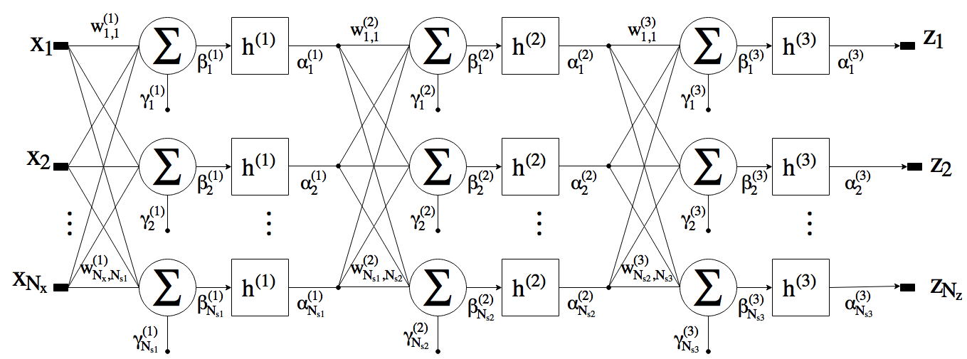
Figure 2: Three-layer feedforward network.

2.3.1 Forward stage

For a network with $\mathcal{L}$ layers the output nodes can be computed using the following recursive matrix relation:

$$\boldsymbol{\alpha}^{(n)}=\begin{cases}\mathbf{x}&n=0;\\ \mathbf{h}^{(n)}(W^{(n)}\boldsymbol{\alpha}^{(n-1)}+\boldsymbol{\gamma}^{(n)})&n=1,\ldots,\mathcal{L},\end{cases}$$ (8)

where, for the $n$-th layer, $W^{(n)}$ is a matrix containing the weights $w^{(n)}_{i,j}$, $\boldsymbol{\gamma}^{(n)}$ is a vector containing the the bias terms $\gamma^{(n)}_{i}$ and $\mathbf{h}^{(n)}$ applies the nonlinear function $h^{(n)}$ element-wise. The output $\mathbf{z}$ is given by:

$$\mathbf{z}=\boldsymbol{\alpha}^{(\mathcal{L})}.$$ (9)

2.3.2 Backward stage

The follow recurrence relation can be used to compute $\tfrac{\partial\mathbf{z}}{\partial\boldsymbol{\beta}^{(n)}}$ for every $n$:

$$\frac{\partial\mathbf{z}}{\partial\boldsymbol{\beta}^{(n)}}=\begin{cases}\dot{H}^{(\mathcal{L})}\big{(}\boldsymbol{\beta}^{(\mathcal{L})}\big{)}&n=\mathcal{L};\\ \tfrac{\partial\mathbf{z}}{\partial\boldsymbol{\beta}^{(n+1)}}\cdot W^{(n+1)}\cdot\dot{H}^{(n)}\big{(}\boldsymbol{\beta}^{(n)}\big{)}&n=\mathcal{L}-1,\ldots,1.\end{cases}$$ (10)

where $\dot{H}^{(n)}$ is given by the following diagonal matrix:

$$\dot{H}^{(n)}\big{(}\boldsymbol{\beta}^{(n)}\big{)}=\text{diag}\Big{(}\dot{h}^{(n)}\big{(}\boldsymbol{\beta}^{(n)}_{1}\big{)},\cdots,\dot{h}^{(n)}\big{(}\boldsymbol{\beta}^{(n)}_{N_{sk}}\big{)}\Big{)}.$$

The recursive expression (10) follows from applying the chain rule
$\left({\tfrac{\partial\mathbf{z}}{\partial\boldsymbol{\beta}^{(n)}}=\tfrac{\partial\mathbf{z}}{\partial\boldsymbol{\beta}^{(n+1)}}\tfrac{\partial\boldsymbol{\beta}^{(n+1)}}{\partial\boldsymbol{\alpha}^{(n)}}\tfrac{\partial\boldsymbol{\alpha}^{(n)}}{\partial\boldsymbol{\beta}^{(n)}}}\right)$, and considering ${\tfrac{\partial\boldsymbol{\beta}^{(n+1)}}{\partial\boldsymbol{\alpha}^{(n)}}=W^{(n+1)}}$ and ${\tfrac{\partial\boldsymbol{\alpha}^{(n)}}{\partial\boldsymbol{\beta}^{(n)}}=\dot{H}^{(n)}}$.

2.3.3 Computing derivatives

The derivatives of $\mathbf{z}$ with respect to $w^{(n)}_{i,j}$ and $\gamma^{(n)}_{i}$ can be used to form the Jacobian matrix $\tfrac{\partial\mathbf{z}}{\partial\mathbf{\Theta}}$ and can be computed using the following expressions:

$$\tfrac{\partial\mathbf{z}}{\partial w^{(n)}_{i,j}} = \tfrac{\partial\mathbf{z}}{\partial\beta^{(n)}_{i}}\tfrac{\partial\beta^{(n)}_{i}}{\partial w^{(n)}_{i,j}}=\tfrac{\partial\mathbf{z}}{\partial\beta^{(n)}_{i}}\alpha^{(n-1)}_{j};$$ (11)

$$\tfrac{\partial\mathbf{z}}{\partial\gamma_{i}^{(n)}} = \tfrac{\partial\mathbf{z}}{\partial\beta^{(n)}_{i}}\tfrac{\partial\beta^{(n)}_{i}}{\partial\gamma_{i}^{(n)}}=\tfrac{\partial\mathbf{z}}{\partial\beta^{(n)}_{i}}.$$ (12)

Furthermore, the derivatives of $\mathbf{z}$ with respect to the inputs $\mathbf{x}$ are:

$$\tfrac{\partial\mathbf{z}}{\partial\mathbf{x}}=\tfrac{\partial\mathbf{z}}{\partial\boldsymbol{\beta}^{(1)}}\tfrac{\partial\boldsymbol{\beta}^{(1)}}{\partial\boldsymbol{\alpha}^{(0)}}=\tfrac{\partial\mathbf{z}}{\partial\boldsymbol{\beta}^{(1)}}W^{(1)}.$$ (13)

The backpropagation algorithm presented here can be directly applied to series-parallel training. For parallel training, however, a different procedure is needed. A recurrent formula for that is introduced in the following section.

3 Training

Unlike other machine learning applications (e.g. natural language processing and computer vision) where there are enormous datasets available to train neural network models, the datasets available for system identification are usually of moderate size. The available data is usually obtained through tests with limited duration because of practical and economical reasons. And, even when there is a long record of input-output data, it either does not contain meaningful dynamic behavior [25] or the system cannot be considered time-invariant over the entire record, resulting in the necessity of selecting smaller portions of this longer dataset for training.

Because large datasets are seldom available in system identification problems, neural networks for such applications are usually restricted to a few hundred weights. The Levenberg-Marquardt method does provide a fast convergence rate [30] and has been described as very efficient for batch training of moderate size problems [27], where the memory used by this algorithm is not prohibitive. Hence, it will be the method of choice for training neural networks in this paper.

Besides that, recurrent neural networks often present vanishing gradients that may prevent the progress of the optimization algorithm. The use of second-order information (as in the Levenberg-Marquardt algorithm) helps to mitigate this problem [31].

In the series-parallel configuration the parameters are estimated by minimizing $\tfrac{1}{2}\|\mathbf{e}_{1}\|^{2}$, what can be done using the algorithm described in Section 2.2. The required Jacobian matrix $\tfrac{\partial\mathbf{e}_{1}}{\partial\mathbf{\Theta}}$ can be computed according to the following well known result.

Proposition 1.

The Jacobian matrix of $\mathbf{e}_{1}$ with respect to $\mathbf{\Theta}$ is
$\tfrac{\partial\mathbf{e}_{1}}{\partial\mathbf{\Theta}}=\left[\tfrac{\partial\mathbf{e}_{1}[1]}{\partial\mathbf{\Theta}}^{T},\cdots,\tfrac{\partial\mathbf{e}_{1}[N]}{\partial\mathbf{\Theta}}^{T}\right]^{T}$, where ${\tfrac{\partial\mathbf{e}_{1}[k]}{\partial\mathbf{\Theta}}=\tfrac{\partial\hat{\mathbf{y}}_{1}[k]}{\partial\mathbf{\Theta}}=\tfrac{\partial\mathbf{F}}{\partial\mathbf{\Theta}}(\underline{\mathbf{y}}_{[k]},\underline{\mathbf{u}}_{[k]};\mathbf{\Theta})}$ that can be computed using the backpropagation described in Section 2.3.

Proof.

This results readily from differentiating (2). ∎

In the parallel configuration the parameters are estimated by minimizing $\tfrac{1}{2}\|\mathbf{e}_{s}\|^{2}$. There are two different ways to take into account the initial conditions ${\underline{\mathbf{y}}_{0}}$: (i) by fixing $\underline{\mathbf{y}}_{0}$ and estimating $\mathbf{\Theta}$; and, (ii) by defining an extended parameter vector ${\mathbf{\Phi}=[\mathbf{\Theta}^{T},\underline{\mathbf{y}}_{0}^{T}]^{T}}$ and estimating $\underline{\mathbf{y}}_{0}$ and $\mathbf{\Theta}$ simultaneously.

When using formulation (i), a suitable choice is to set the initial conditions equal to the measured outputs (${\mathbf{y}_{0}[k]=\mathbf{y}[k],~{}k=1,\ldots,n_{y}}$). When using formulation (ii) the measured output vector may be used as an initial guess that will be refined by the optimization algorithm.

The optimal choice for the initial condition would be ${\mathbf{y}_{0}[k]=\mathbf{y}^{*}[k]}$ for
${k=1,\cdots,n_{y}}$. Formulation (i) uses the non-optimal choice ${\mathbf{y}_{0}[k]=\mathbf{y}[k]\neq\mathbf{y}^{*}[k]}$. Formulation (ii) goes one step further and include the initial conditions $\mathbf{y}_{0}[k]$ in the optimization problem, so it converges to $\mathbf{y}^{*}[k]$ and hence improves the parameter estimation.

The required Jacobian matrices $\tfrac{\partial\mathbf{e}_{s}}{\partial\mathbf{\Theta}}$ and $\tfrac{\partial\mathbf{e}_{s}}{\partial\underline{\mathbf{y}}_{0}}$ can be computed according to the following proposition.

Proposition 2.

The Jacobian matrices of $\mathbf{e}_{1}$ with respect to $\mathbf{\Theta}$ and $\underline{\mathbf{y}}_{0}$ are ${\tfrac{\partial\mathbf{e}_{s}}{\partial\mathbf{\Theta}}=\left[\tfrac{\partial\mathbf{e}_{s}[1]}{\partial\mathbf{\Theta}}^{T},\cdots,\tfrac{\partial\mathbf{e}_{s}[N]}{\partial\mathbf{\Theta}}^{T}\right]^{T}}$ and ${\tfrac{\partial\mathbf{e}_{s}}{\partial\underline{\mathbf{y}}_{0}}=\left[\tfrac{\partial\mathbf{e}_{s}[1]}{\partial\underline{\mathbf{y}}_{0}}^{T},\cdots,\tfrac{\partial\mathbf{e}_{s}[N]}{\partial\underline{\mathbf{y}}_{0}}^{T}\right]^{T}}$ where ${\tfrac{\partial\mathbf{e}_{s}[k]}{\partial\mathbf{\Theta}}=\tfrac{\partial\hat{\mathbf{y}}_{s}[k]}{\partial\mathbf{\Theta}}}$ and ${\tfrac{\partial\mathbf{e}_{s}[k]}{\partial\underline{\mathbf{y}}_{0}}=\tfrac{\partial\hat{\mathbf{y}}_{s}[k]}{\partial\underline{\mathbf{y}}_{0}}}$ can be computed according to the following recursive formulas:

$$\frac{\partial\hat{\mathbf{y}}_{s}[k]}{\partial\mathbf{\Theta}}=\begin{dcases}\mathbf{0},~{}1\leq k\leq n_{y};\\ \begin{split}\tfrac{\partial\mathbf{F}}{\partial\mathbf{\Theta}}(\hat{\mathbf{y}}_{[k]},\mathbf{u};_{[k]}\mathbf{\Theta})+\sum_{i=1}^{n_{y}}\tfrac{\partial\mathbf{F}}{\partial\mathbf{y}[k-i]}(\hat{\mathbf{y}}_{[k]},\mathbf{u}_{[k]};&\mathbf{\Theta})\tfrac{\partial\hat{\mathbf{y}}_{s}[k-i]}{\partial\mathbf{\Theta}},\\ &k>n_{y},\end{split}\end{dcases}$$ (14)

$$\frac{\partial\hat{\mathbf{y}}_{s}[k]}{\partial\underline{\mathbf{y}}_{0}}=\begin{dcases}D^{(n)},~{}1\leq k\leq n_{y};\\ \begin{split}\sum_{i=1}^{n_{y}}&\tfrac{\partial\mathbf{F}}{\partial\mathbf{y}[k-i]}(\hat{\mathbf{y}}_{[k]},\mathbf{u}_{[k]};\mathbf{\Theta})\tfrac{\partial\hat{\mathbf{y}}_{s}[k-i]}{\partial\underline{\mathbf{y}}_{0}},~{}k>n_{y},\end{split}\end{dcases}$$ (15)

where $D^{(n)}\in\mathbb{R}^{N_{y}\times n_{y}N_{y}}$ is defined as:

$$\big{\{}D^{(n)}\big{\}}_{i,j}=\begin{dcases}1,&\text{if }j=(n-1)\cdot N_{y}+i,\\ 0,&\text{otherwise.}\end{dcases}$$ (16)

Proof.

The proof follows from differentiating (3) and applying the chain rule. ∎

This formula can be interpreted either as a variation of the dynamic backpropagation [1] adapted to compute the Jacobian instead of the gradient; or, as a specific case of real-time recurrent learning [32] with a special type of recurrent connection.

4 Complexity analysis

In this section we present a novel complexity analysis comparing series-parallel training (SP), parallel training with fixed initial conditions (P$\mathbf{\Theta}$) and parallel training with extended parameter vector (P$\mathbf{\Phi}$). We show that the training methods have similar computational cost for the nonlinear least-squares formulation. The number of floating point operations (flops) is estimated based on [33, Table 1.1.2]. Low-order terms, as usual, are neglected in the analysis.

4.1 Neural network output and its partial derivatives

The backpropagation algorithm described in Section 2.3 can be used for training both fully or partially connected networks. The differences relate to the internal representation of the weight matrices $W^{(n)}$: for a partially connected network the matrices are stored using a sparse representation, e.g. compressed sparse column (CSC) representation.

The total number of flops required to evaluate the output and to compute partial derivatives for a fully connected feedforward network is summarized in Table 1. $N_{w}$ and $N_{\gamma}$ are respectively the total number of weights and of bias terms, such that $N_{w}+N_{\gamma}=N_{\Theta}$. For this fully connected network:

$$N_{w} = N_{x}\cdot N_{s1}+N_{s1}\cdot N_{s2}+\cdots+N_{s(\mathcal{L}-1)}\cdot N_{s\mathcal{L}},$$

$$N_{\gamma} = N_{s1}+N_{s2}+\cdots+N_{s\mathcal{L}}.$$ (17)

Table 1: Modified backpropagation number of flops for a fully connected network.

Computing Neural Network Output
i) Compute $\mathbf{F(\mathbf{x};\mathbf{\Theta})}$ — Eq. (8)-(9)	$2N_{w}$
Computing Partial Derivatives
ii) Backward Stage — Eq. (10)	$(2N_{z}+1)(N_{w}-N_{x}N_{s1})$
iii) Compute $\tfrac{\partial\mathbf{F}}{\partial\mathbf{\Theta}}$ — Eq. (11)-(12)	$N_{w}\cdot N_{z}$
iv) Compute $\tfrac{\partial\mathbf{F}}{\partial\mathbf{x}}$ — Eq. (13)	$2N_{x}\cdot N_{s1}\cdot N_{z}$

Since the more relevant terms of the complexity analysis in Table 1 are being expressed in terms of the number of weights $N_{w}$ the results for a fully connected network are similar to the ones that would be obtained for a partially connected network using a sparse representation.

4.2 Number of flops for series-parallel and parallel training

Table 2: Levenberg-Marquardt number of flops per iteration for series-parallel training (SP), parallel training with fixed initial conditions (P$\mathbf{\Theta}$) and parallel training with extended parameter vector (P$\mathbf{\Phi}$). A mark ✗ signals which calculation is required in each method.

		SP	P$\mathbf{\Theta}$	P$\mathbf{\Phi}$
Computing Error
i) Compute $\mathbf{F(\mathbf{x};\mathbf{\Theta})}$	$2N\cdot N_{w}$	✗	✗	✗
Computing Partial Derivatives
ii) Backward Stage	$N(2N_{y}+1)(N_{w}-N_{x}N_{s1})$	✗	✗	✗
iii) Compute $\tfrac{\partial\mathbf{F}}{\partial\mathbf{\Theta}}$	$N\cdot N_{w}\cdot N_{y}$	✗	✗	✗
iv) Compute $\tfrac{\partial\mathbf{F}}{\partial\mathbf{x}}$	$2N\cdot N_{x}\cdot N_{s1}\cdot N_{y}$		✗	✗
v) Equation (14)	$2N\cdot N_{\Theta}\cdot(N_{y}^{2}+N_{y})$		✗	✗
vi) Equation (15)	$2N\cdot n_{y}\cdot N_{y}\cdot(N_{y}^{2}+N_{y})$			✗
Solving Equation (6)
vii) Solve (6) — $\mathbf{\Theta}$	$2N\cdot N_{\Theta}^{2}+\tfrac{1}{3}N_{\Theta}^{3}$	✗	✗
viii) Solve (6) — $\mathbf{\Phi}$	$2N\cdot N_{\Phi}^{2}+\tfrac{1}{3}N_{\Phi}^{3}$			✗

The number of flops of each iteration of the Levenberg-Marquardt algorithm is summarized in Table 2. Entries (i) to (iv) in Table 2 follow directly from Table 1, considering ${N_{z}=N_{y}}$ and multiplying the costs by $N$ because of the number of different inputs being evaluated. Furthermore, in entries (v) and (vi) the evaluation of (14) and (15) is accomplished by storing computed values and performing only one new matrix-matrix product per evaluation.

The cost of solving (6) is about $2\cdot N\cdot N_{\Theta}^{2}+\tfrac{1}{3}\cdot N_{\Theta}^{3}$ where the cost $2N\cdot N_{\Theta}^{2}$ is due to the multiplication of the Jacobian matrix by its transpose and $\tfrac{1}{3}N_{\Theta}^{3}$ is due to the needed Cholesky factorization. When using an extended parameter vector, $N_{\Theta}$ is replaced with $N_{\Phi}$ in the analysis.

4.3 Comparing methods

Assuming the number of nodes in the last hidden layer is greater than the number of outputs ($N_{y}<N_{s(\mathcal{L}-1)}$), the inequalities apply:

$$n_{y}\cdot N_{y}\leq N_{x}<N_{x}\cdot N_{s1}\leq N_{w}<N_{\Theta};$$ (18)

$$N_{y}<N_{y}^{2}<N_{y}\cdot N_{s(\mathcal{L}-1)}\leq N_{w}<N_{\Theta}.$$

From Table 2 and from the above inequalities it follows that the cost of each Levenberg-Marquardt iteration is dominated by the cost of solving Equation (6). Furthermore, ${N_{\Phi}=N_{\Theta}+n_{y}\cdot N_{y}<2N_{\Theta}}$, hence, the asymptotic computational cost of the training method S$\mathbf{\Phi}$ is the same as that of SP and S$\mathbf{\Theta}$ methods: ${\mathcal{O}(N\cdot N_{\Theta}^{2}+N_{\Theta}^{3})}$.

From Table 2 it is also possible to analyze the cost of each of the major steps needed in each full iteration of the algorithm:

• Computing Error: The cost of computing the error is the same for all of the training methods.

• Computing Partial Derivatives: The computation of partial derivatives has a cost of $\mathcal{O}(N\cdot N_{w}\cdot N_{y})$ for the SP training method and a cost of $\mathcal{O}(N\cdot N_{\Theta}\cdot N_{y}^{2})$ for both P$\mathbf{\Phi}$ and P$\mathbf{\Theta}$. For many cases of interest in system identification, the number of model outputs $N_{y}$ is small. Furthermore, ${N_{\Theta}=N_{w}+N_{\gamma}\approx N_{w}}$ (see Eq. (17)). That is why the cost of computing the partial derivatives for parallel training is comparable to the cost for series-parallel training.

• Solving Equation (6): It already has been established that the cost of this step $\mathcal{O}(N\cdot N_{\Theta}^{2}+N_{\Theta}^{3})$ dominates the computational cost for all the training methods. Furthermore $n_{y}\cdot N_{y}$ is usually much smaller than $N_{\Theta}$ such that $N_{\Phi}\approx N_{\Theta}$ and the number of flops of this stage is basically the same for all the training methods.

4.4 Memory complexity

Considering that $N\gg n_{y}$ , it follows that, for the three training methods, the storage capacity is dominated by the storage of the Jacobian matrix ${\tfrac{\partial\mathbf{e}}{\partial\mathbf{\Theta}}}$ or of the matrix resulting from the product ${\left[\tfrac{\partial\mathbf{e}}{\partial\mathbf{\Theta}}\right]^{T}\left[\tfrac{\partial\mathbf{e}}{\partial\mathbf{\Theta}}\right]}$. Therefore the memory size required by the algorithm is about $\mathcal{O}(\max(N\cdot N_{y}\cdot N_{\Theta},~{}N_{\Theta}^{2}))$.

For very large datasets and a large number of parameters, this storage requirement may be prohibitive and others methods should be used (e.g. stochastic gradient descent or variations). Nevertheless, for datasets of moderate size and networks with few hundred parameters, as it is usually the case for system identification, the use of nonlinear least-squares is a viable option.

5 Unifying framework

In this section we present parallel and series-parallel training in the prediction error methods framework [34, 35]. This analysis provides some insight about the situations in which one training method outperforms the other one.

5.1 Output error vs equation error

To study the previously described problem it is assumed that for a given input sequence ${\mathbf{u}[k]}$ and a set of initial conditions ${\mathbf{y}^{*}_{0}}$ the output was generated by a “true system”, described by the following equations:

$$\mathbf{y}^{*}[k]= \mathbf{F}^{*}(\mathbf{y}^{*}[k-1],\ldots,\mathbf{y}^{*}[k-n_{y}],\mathbf{u}[k-\tau_{d}],\ldots,\mathbf{u}[k-n_{u}];\mathbf{\Theta}^{*})+\mathbf{v}[k]$$

$$\mathbf{y}[k]= \mathbf{y}^{*}[k]+\mathbf{w}[k],$$ (19)

where $\mathbf{F}^{*}$ and $\mathbf{\Theta}^{*}$ are the “true” function and parameter vector that describe the system; $\mathbf{v}[k]\in\mathbb{R}^{N_{y}}$ and ${\mathbf{w}[k]\in\mathbb{R}^{N_{y}}}$ are random variable vectors, that cause the deviation of the deterministic model from its true value; $\mathbf{u}[k]$ and $\mathbf{y}[k]$ are the measured input and output vectors; and, $\mathbf{y}^{*}[k]$ is the output vector without the effect of the output error.

The random variable $\mathbf{v}[k]$ affects the system dynamics and is called equation error, while the random variable $\mathbf{w}[k]$ only affects the measured values and is called output error.

5.2 Optimal predictor

If the measured values of $\mathbf{y}$ and $\mathbf{u}$ are known at all instants previous to $k$, the optimal prediction of $\mathbf{y}[k]$ is the following conditional expectation:

$$\hat{\mathbf{y}}_{*}[k]=E\left\{\mathbf{y}[k]~{}\Big{|}~{}\underline{\mathbf{y}}_{[k]},\underline{\mathbf{u}}_{[k]}\right\}$$ (20)

where $\hat{\mathbf{y}}_{*}[k]$ denotes the optimal prediction and $E\{\cdot\}$ indicates the mathematical expectation.

Consider the following situations:

Situation 1 (White equation error).

The sequence of equation errors $\{\mathbf{v}[k]\}$ is a white noise process and the output error is zero $({\mathbf{w}[k]=0})$.

Situation 2 (White output error).

The sequence of output errors $\{\mathbf{w}[k]\}$ is a white noise process and the equation error is zero $(\mathbf{v}[k]=0)$.

The next two lemmas give the optimal prediction $\hat{\mathbf{y}}_{*}[k]$ for the two situations above:

Lemma 1.

If Situation 1 holds and the function and parameter vector matches the true ones $(\mathbf{F}=\mathbf{F}^{*}$ and $\mathbf{\Theta}=\mathbf{\Theta}^{*})$, then the one-step-ahead prediction is equal to the optimal prediction $(\hat{\mathbf{y}}_{1}[k]=\hat{\mathbf{y}}_{*}[k])$.

Proof.

Since the output error is zero, it follows that $\mathbf{y}[k]=\mathbf{y}^{*}[k]$ and therefore Equation (19) reduces to $\mathbf{y}[k]=\mathbf{F}^{*}(\underline{\mathbf{y}}_{[k]},\underline{\mathbf{u}}_{[k]};\mathbf{\Theta}^{*})+\mathbf{v}[k]$.

And, because $\mathbf{v}[k]$ has zero mean, it follows that:

$$\hat{\mathbf{y}}_{*}[k]=E\{\mathbf{y}[k]\,\mid\,\underline{\mathbf{y}}_{[k]},\underline{\mathbf{u}}_{[k]}\}=\mathbf{F}^{*}(\underline{\mathbf{y}}_{[k]},\underline{\mathbf{u}}_{[k]};\mathbf{\Theta}^{*})=\hat{\mathbf{y}}_{1}[k].$$

∎

Lemma 2.

If Situation 2 holds, and the function, parameter vector and initial conditions matches the true ones $(\mathbf{F}=\mathbf{F}^{*}$, $\mathbf{\Theta}=\mathbf{\Theta}^{*}$ and $\mathbf{y}_{0}=\mathbf{y}^{*}_{0})$, then the free-run simulation is the optimal prediction $(\hat{\mathbf{y}}_{s}[k]=\hat{\mathbf{y}}_{*}[k])$.

Proof.

There is no equation error and therefore:

$$\hat{\mathbf{y}}_{*}[k]=E\{\mathbf{y}[k]\,\mid\,\underline{\mathbf{y}}_{[k]},\underline{\mathbf{u}}_{[k]}\}=E\{\mathbf{y}^{*}[k]+\mathbf{w}[k]\,\mid\,\underline{\mathbf{y}}_{[k]},\underline{\mathbf{u}}_{[k]}\}=\mathbf{y}^{*}[k]=\hat{\mathbf{y}}_{s}[k],$$

where it was used that for matching initial conditions and parameters and in the absence of equation error, the noise-free output ${\mathbf{y}^{*}[k]}$ is exactly equal to the free-run simulation (${\mathbf{y}^{*}[k]=\hat{\mathbf{y}}_{s}[k]}$). ∎

Hence, for $\mathbf{F}=\mathbf{F}^{*}$, both training methods minimize an error that approaches the optimal predictor error ${\mathbf{e}_{*}[k]=\hat{\mathbf{y}}_{*}[k]-\mathbf{y}[k]}$ as $\mathbf{\Theta}\rightarrow\mathbf{\Theta}^{*}$. Series-parallel training does it for Situation 1, and parallel training for Situation 2. It follows from [34] that, under additional assumptions, series-parallel training is a consistent estimator for Situation 1 and parallel training is a consistent estimator for Situation 2.

6 Implementation and test results

The implementation is in Julia and runs on a computer with a processor Intel(R) Core(TM) i7-4790K CPU @ 4.00GHz. For all examples in this paper, the activation function used in hidden layers is the hyperbolic tangent, the initial values of the weights $w_{i,j}^{(n)}$ are drawn from a zero mean normal distribution with standard deviation ${\sigma=(N_{s(n)})^{-0.5}}$ and the bias terms $\gamma_{i}^{(n)}$ are initialized with zeros [37]. Also, in all parallel training examples the parameter vector is extended with the initial conditions for the optimization process (P$\Phi$ training).

The free-run mean-square simulation error (${\text{MSE}=\tfrac{1}{N}\sum_{n=1}^{N}(y[k]-\hat{y}[k])^{2}}$) is used to compare the models over the validation window.

The first example compares the training method using data from an experimental plant and the second one investigates different noise configurations on computer generated data. The code and data used in the numerical examples are available.

6.1 Example 1: Data from a pilot plant

In this example, input-output signals were collected from LabVolt Level Process Station (model 3503-MO [38]). This plant consists of a tank that is filled with water from a reservoir. The water is pumped at fixed speed, while the flow is regulated using a pneumatically operated control valve driven by a voltage $u[k]$. The water column height $y[k]$ is indirectly measured using a pressure sensor at the bottom of the tank. Figure 3 shows the free-run simulation over the validation window of models obtained for this process using parallel and series-parallel training.

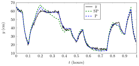
Figure 3: Validation window for pilot plant. Free-run simulation for models obtained using series-parallel (SP) and parallel (P) training. The mean square errors are ${\text{MSE}_{\text{SP}}=1144.6}$; ${\text{MSE}_{\text{P}}=296.2}$. The models have ${n_{y}=n_{u}=1}$ and 10 nodes in the hidden layer and were trained on a two hour long dataset sampled at $T_{s}=10{\rm s}$. The same initial parameter guess was used for both training methods. The training was 100 epochs long, which took 3.3 and 3.9 s, respectively, for series-parallel and parallel training.

Since parameters are randomly initialized, different realizations will yield different results. Figure 4 shows the validation errors for both training methods for randomly drawn initial guesses. While parallel training consistently provides models with better validation results than series-parallel training, it also has some outliers that result in very poor validation results. Such outliers probably happen as the algorithm gets trapped in “poor” local minima during parallel training.

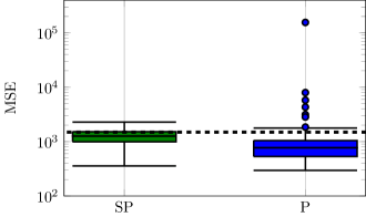
Figure 4: Boxplots show the distribution of the free-run simulation MSE over the validation window for models trained using series-parallel (SP) and parallel (P) methods under the circumstances specified in Figure 3. There are 100 realizations of the training in each boxplot, for each realization the weights $w_{i,j}^{(n)}$ are drawn from a normal distribution with zero mean standard deviation ${\sigma=(N_{s(n-1)})^{-0.5}}$ and the bias terms $\gamma_{i}^{(n)}$ are initialized with zeros [37]. For comparison purposes, the dashed horizontal line gives the performance of an ARX linear model ($n_{y}=1$ and $n_{u}=1$) trained and tested under the same conditions.

The training of the neural network was performed using normalized data. However, if unscaled data were used instead, parallel training would yield models with ${\text{MSE}>10000}$ over the validation window while series-parallel training can still yield solutions with a reasonable fit to the validation data. We understand this as another indicator of parallel training greater sensitivity to the initial parameter guess: for unscaled data, the initial guess is far away from meaningful solutions of the problem, and, while series-parallel training converges to acceptable results, parallel training gets trapped in “poor” local solutions.

6.2 Example 2: Investigating the noise effect

The non-linear system: [2]:

$$y^{*}[k] = (0.8-0.5e^{-y^{*}[k-1]^{2}})y^{*}[k-1]-$$

$$(0.3+0.9e^{-y^{*}[k-1]^{2}})y^{*}[k-2]+u[k-1]+$$

$$0.2u[k-2]+0.1u[k-1]u[k-2]+v[k]$$

$$y[k] = y^{*}[k]+w[k],$$ (21)

was simulated and the generated dataset was used to build neural network models. Figure 5 shows the validation results for models obtained for a training set generated with white Gaussian equation and output errors $v$ and $w$. In this section, we repeat this same experiment for diverse random processes applied to $v$ and $w$ in order to investigate how different noise configurations affect parallel and series-parallel training.

Figure 5: Displays the first 100 samples of the free-run simulation in the validation window for models trained using series-parallel (SP) and parallel (P) methods. The mean square errors are ${\text{MSE}_{\text{SP}}=0.39}$; ${\text{MSE}_{\text{P}}=0.06}$. The models have ${n_{y}=n_{u}=2}$ and a single hidden layer with 10 nodes. The training set has $N=1000$ samples and was generated with (21) for $v$ and $w$ white Gaussian noise with standard deviations $\sigma_{v}=0.1$ and $\sigma_{w}=0.5$. The validation window is generated without the noise effect. For both, the input $u$ is randomly generated with standard Gaussian distribution, each randomly generated value held for 5 samples. The training was 100 epochs long, which took 5.0 and 6.1 s for, respectively, series-parallel and parallel training.

6.2.1 White noise

Let $v$ be white Gaussian noise with standard deviation ${\sigma_{v}}$ and let $w$ be zero. Figure 6 (a) shows the free-run simulation error on the validation window using parallel and series-parallel training for increasing values of ${\sigma_{v}}$. Figure 6 (b) shows the complementary experiment, for which $v$ is zero and $w$ is white Gaussian noise with increasing larger values of ${\sigma_{w}}$ being tried out.

In Section 5, series-parallel training was derived considering the presence of white equation error and, in this situation, the numerical results illustrate the model obtained using this training method presents the best validation results (Figure 6 (a)). On the other hand, parallel training was derived considering the presence of white output error and is significantly better in this alternative situation (Figure 6 (b)).

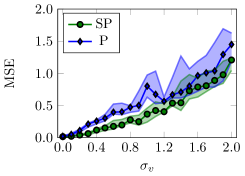
(a)

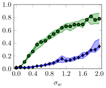
(b)

Figure 6: Free-run simulation MSE on the validation window vs noise levels for series-parallel and parallel training. The main line indicates the median and the shaded region indicates interquartile range. These statistics were computed from 12 realizations. In (a) $v$ is a Gaussian white process and $w=0$; and, in (b) $w$ is a Gaussian white process and $v=0$.

6.2.2 Colored noise

Consider $w=0$ and $v$ a white Gaussian noise filtered by a low pass filter with cutoff frequency $\omega_{c}$. Figure 7 shows the free-run simulation error in the validation window for both parallel and series-parallel training for a sequence of values of $\omega_{c}$ and different noise intensities. The result indicates parallel training provides the best results unless the equation error has a very large bandwidth.

More extensive tests are summarized in Table 3, which shows the validation errors for a training set with colored Gaussian errors in different frequency bands. Again, except for white or large bandwidth equation error, parallel training seems to provide the smallest validation errors.

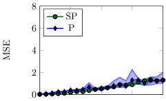
(a) $\omega_{c}=0.8$

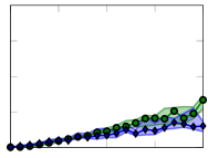
(b) $\omega_{c}=0.6$

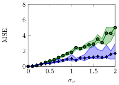
(c) $\omega_{c}=0.4$

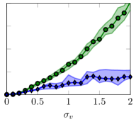
(d) $\omega_{c}=0.2$

Figure 7: Free-run simulation MSE over the validation window vs standard deviation of colored equation error. The output error $w=0$ and the equation error $v$ is a colored Gaussian noise obtained by applying a 4th-order lowpass Butterworth filter with cutoff frequency $\omega_{c}$ to white Gaussian noise in both the forward and reverse directions. The figure shows the result for different values of $\omega_{c}$, where $\omega_{c}$ is the normalized frequency (with $\omega_{c}=1$ the Nyquist frequency). The main line indicates the median and the shaded region indicates interquartile range. These statistics were computed from 12 realizations.

Equation error can be interpreted as the effect of unaccounted inputs and unmodeled dynamics, hence situations where this error is not auto-correlated are very unlikely. Therefore, the only situations we found series-parallel training to perform better (when the equation error power spectral density occupy almost the whole frequency spectrum) seem unlikely to appear in practice. This may justify parallel training to produce better models for real application problems as the pilot plant in Example 1, the battery modeling described in [24], or the boiler unit in [23].

Table 3: Free-run simulation MSE on the validation window for parallel and series-parallel training. Both the mean and the standard deviation are displayed (30% trimmed estimation computed from 12 realizations). In situation (a), the training data was generated with zero output error ($w=0$) and $v$ is a Gaussian random process. In (b), the training data was generated with $v=0$ and $w$ is a Gaussian random process. The Gaussian random process has standard deviation $\sigma=1.0$ and power spectral density confined to the given frequency band. In both situations, the rows where the frequency ranges from $0.0$ to $1.0$ (the whole spectrum) corresponds to white noise, in the remaining rows we apply a 4th-order lowpass (or highpass) Butterworth filter to white Gaussian noise (in both the forward and reverse directions) in order to obtain the signal in the desired frequency band. The cell of the training method with the best validation results between the two models is colored. Its colored red when the difference in the MSE is larger than the sum of standard deviations and yellow when it is not.

	(a)  $v\not=0$, $w=0$		(b)  $w\not=0$, $v=0$
$\omega$ range	SP	P	SP	P
$0.0\rightarrow 1.0$	$0.36\pm 0.09$	$0.78\pm 0.18$	$0.58\pm 0.03$	$0.13\pm 0.03$
$0.0\rightarrow 0.8$	$0.53\pm 0.13$	$0.58\pm 0.10$	$0.44\pm 0.02$	$0.12\pm 0.03$
$0.0\rightarrow 0.6$	$0.94\pm 0.13$	$0.75\pm 0.23$	$0.30\pm 0.05$	$0.15\pm 0.05$
$0.0\rightarrow 0.4$	$1.86\pm 0.20$	$1.07\pm 0.38$	$0.46\pm 0.05$	$0.15\pm 0.02$
$0.0\rightarrow 0.2$	$2.60\pm 0.26$	$1.16\pm 0.44$	$0.71\pm 0.05$	$0.18\pm 0.04$
$0.0\rightarrow 1.0$	$0.36\pm 0.09$	$0.78\pm 0.18$	$0.58\pm 0.03$	$0.13\pm 0.03$
$0.2\rightarrow 1.0$	$0.52\pm 0.07$	$0.57\pm 0.12$	$0.59\pm 0.03$	$0.09\pm 0.02$
$0.4\rightarrow 1.0$	$0.57\pm 0.08$	$0.22\pm 0.05$	$0.63\pm 0.05$	$0.05\pm 0.01$
$0.6\rightarrow 1.0$	$0.54\pm 0.07$	$0.21\pm 0.01$	$0.68\pm 0.03$	$0.03\pm 0.02$
$0.8\rightarrow 1.0$	$0.58\pm 0.05$	$0.17\pm 0.04$	$0.78\pm 0.09$	$0.03\pm 0.01$

6.3 Running time

In Section 4 we find out the computational complexity of $\mathcal{O}(N\cdot N_{\Theta}^{2}+N_{\Theta}^{3})$. The first term $\mathcal{O}(N\cdot N_{\Theta}^{2})$ seems to dominate and in Figure 8 we show that the running time grows linearly with the number of training samples $N$ and quadratically with the number of parameters $N_{\Theta}$.

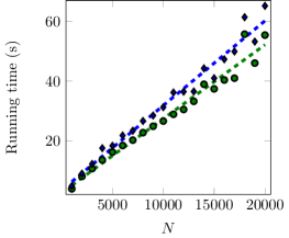
(a)

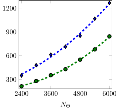
(b)

Figure 8: Running time (in seconds) of training (100 epochs). The average running time of 5 realizations is displayed for series-parallel training () and for parallel training (). The neural network has a single hidden layer and a total of $N_{\Theta}$ parameters to be estimated. The training set has $N$ samples and was generated as described in Figure 5. In (a), we fix $N_{\Theta}=61$ and plot the timings as a function of the number of training samples $N$, a line is adjusted to illustrate the running time grows linearly with the training size for both training methods. In (b), we fix $N=10000$ and plot the timings as a function of the number of parameters $N_{\Theta}$, a second order polynomial is adjusted to illustrate the running time quadratic growth.

The running time growing with the same rate for both training methods implies that the ratio between series-parallel and parallel training running time is bounded by a constant. For the examples we presented in this paper the parallel training takes about 20% longer than series-parallel training. Hence the difference of running times for sequential execution does not justify the use of one method over the other.

7 Discussion

7.1 Convergence towards a local minima

The optimization problem that results from both series-parallel and parallel training of neural networks are non-convex and may have multiple local minima. The solution of the Levenberg-Marquardt algorithm discussed in this paper, as well as most algorithms of interest for training neural networks (e.g. stochastic gradient descent, L-BFGS, conjugate gradient), converges towards a local minimum. However, there is no guarantee for neither series-parallel nor parallel training that the solution found is the global optimum. The convergence to “poor” local solutions may happen for both training methods, however, as illustrated in the numerical examples, it seems to happen more often for parallel training.

For the examples presented in this paper the possibility of being trapped in “poor” local solutions is only a small inconvenience, requiring the data to be carefully normalized and, in some rare situations, the model to be retrained. An exception are chaotic systems for which small variations in the parameters may cause great variations in the free-run simulation trajectory, causing the parallel training objective function to be very intricate and full of undesirable local minima.

7.2 Signal unboundedness during training

Signals obtained in intermediary steps of parallel identification may become unbounded. The one-step-ahead predictor, used in series-parallel training, is always bounded since the prediction depends only on measured values – it has a FIR (Finite Impulse Response) structure – while, for the parallel training, the free-run simulation could be unbounded for some choice of parameters because of its dependence on its own past simulation values.

This is a potential problem because during an intermediary stage of parallel training a choice of $\mathbf{\Theta}^{k}$ that results in unbounded values of $\hat{\mathbf{y}}_{s}[k]$ may need to be evaluated, resulting in overflows. Hence, optimization algorithms that may work well minimizing one-step-ahead prediction errors $\mathbf{e}_{1}$, may fail when minimizing simulation errors $\mathbf{e}_{s}$.

For instance, steepest descent algorithms with a fixed step size may, for a poor choice of step size, fall into a region in the parameter space for which the signals are unbounded and the computation of the gradient will suffer from overflow and prevent the algorithm from continuing (since it does not have a direction to follow). This may also happen in more practical line search algorithms (e.g. the one described in [30, Sec. 3.5]).

The Levenberg-Marquardt algorithm, on the other hand, is robust against this kind of problem because every step $\mathbf{\mathbf{\Theta}}^{n}+\mathbf{\Delta}\mathbf{\mathbf{\Theta}}^{n}$ that causes overflow in the objective function computation yields a negative $\rho_{n}$, hence the step is rejected by the algorithm and $\lambda_{n}$ is increased. The increase in $\lambda_{n}$ causes the length of $\mathbf{\Delta}\mathbf{\mathbf{\Theta}}^{n}$ to decrease. Therefore, the step length is decreased until a point is found sufficiently close to the current iteration such that overflow does not occur. Hence, the Levenberg-Marquardt algorithm does not fail or stall due to overflows. Similar reasoning could be used for any trust-region method or for backtracking line-search.

Regardless of the optimization algorithm, signal unboundedness is not a problem for feedforward networks with bounded activation functions (e.g. Logistic or Hyperbolic Tangent) in the hidden layers, because its output is always bounded. Hence parallel training of these particular neural networks is not affected by the previously mentioned difficulties.

7.3 Time series prediction

It is important to highlight that parallel training is inappropriate to train neural networks for predicting time series in general. That is, parallel configuration is generally inadequate for the case when there are no inputs ($N_{u}=0$).

For any asymptotically stable system in parallel configuration, the absence of inputs would make the free-run simulation converge towards an equilibrium, and even models that should be capable of providing good predictions for a few steps-ahead in the time series, may present poor performance for the entire training window. Hence, minimizing $\|\mathbf{e}_{s}\|^{2}$ will not provide good results in general.

It still make sense to use series-parallel training for time series models. That is because, feeding measured values into the neural network keeps it from converging towards zero (for asymptotically stable systems) and makes the estimation robust against unknown disturbances affecting the time series. An interesting approach that mixes parallel and series-parallel training for time series prediction is given in [40].

7.4 Batch vs online training

We have based our analysis on batch training. However, instead of using all the available samples for training at once we could have fed samples one-by-one or chunk-by-chunk to the training algorithm (online training). The choice of parallel or series-parallel training, however, is orthogonal to the choice between online and batch training. And most of the ideas presented in this paper, including: 1) the unified framework; 2) the discussion about poor local minima; and 3) the study of how colored noise affects the parameter estimation; are all applicable to the case of online training.

7.5 Parallelization

For the examples presented here the difference of running times for sequential execution does not justify the use of one method over the other. Furthermore, both methods have the same time complexity. Parallel training is, however, much less amenable to parallelization because of the dependencies introduced by the recursive relations used for computing its error and Jacobian matrix.

8 Conclusion and future work

In this paper we have studied different aspects of parallel training under a nonlinear least squares formulation. Several published works take for granted that series-parallel training always provides better results with lower computational cost. The results presented in this paper show that this is not always the case and that parallel training does provide advantages that justify its use in several situations. The results presented in the numerical examples suggest parallel training can provide models with smaller generalization error than series-parallel training under more realistic scenarios concerning noise. Furthermore, for sequential execution the complexity analysis and the numerical examples suggest the computational cost is not significantly different for both methods in typical system identification problems.

Nevertheless, series-parallel training has two real advantages over parallel training: i) it seems less likely to be trapped in “poor” local solutions; ii) it is more amenable to parallelization. In [41] a technique called multiple shooting is introduced in the framework of prediction error methods as a way of reducing the possibility of parallel training getting trapped in “poor” local minima and also making the algorithm much more amenable to parallelization. It seems to be a promising way to solve the shortcomings of parallel training we have described in this paper.

References

References

- Narendra and Parthasarathy [1990] K. S. Narendra, K. Parthasarathy, Identification and Control of Dynamical Systems Using Neural Networks, IEEE Transactions on Neural Networks 1 (1) (1990) 4–27.
- Chen et al. [1990] S. Chen, S. A. Billings, P. M. Grant, Non-Linear System Identification Using Neural Networks, International Journal of Control 51 (6) (1990) 1191–1214.
- Zhang et al. [2006] D.-y. Zhang, L.-p. Sun, J. Cao, Modeling of Temperature-Humidity for Wood Drying Based on Time-Delay Neural Network, Journal of Forestry Research 17 (2) (2006) 141–144.
- Singh et al. [2013] M. Singh, I. Singh, A. Verma, Identification on Non Linear Series-Parallel Model Using Neural Network, MIT Int. J. Electr. Instrumen. Eng 3 (1) (2013) 21–23.
- Saad et al. [1994] M. Saad, P. Bigras, L.-A. Dessaint, K. Al-Haddad, Adaptive Robot Control Using Neural Networks, IEEE Transactions on Industrial Electronics 41 (2) (1994) 173–181.
- Beale et al. [2017] M. H. Beale, M. T. Hagan, H. B. Demuth, Neural Network Toolbox for Use with MATLAB, Tech. Rep., Mathworks, 2017.
- Saggar et al. [2007] M. Saggar, T. Meriçli, S. Andoni, R. Miikkulainen, System Identification for the Hodgkin-Huxley Model Using Artificial Neural Networks, in: Neural Networks, 2007. IJCNN 2007. International Joint Conference On, IEEE, 2239–2244, 2007.
- Warwick and Craddock [1996] K. Warwick, R. Craddock, An Introduction to Radial Basis Functions for System Identification. A Comparison with Other Neural Network Methods, in: Decision and Control, 1996., Proceedings of the 35th IEEE Conference On, vol. 1, IEEE, 464–469, 1996.
- Kamińnski et al. [1996] W. Kamińnski, P. Strumitto, E. Tomczak, Genetic Algorithms and Artificial Neural Networks for Description of Thermal Deterioration Processes, Drying Technology 14 (9) (1996) 2117–2133.
- Rahman et al. [2000] M. F. Rahman, R. Devanathan, Z. Kuanyi, Neural Network Approach for Linearizing Control of Nonlinear Process Plants, IEEE Transactions on Industrial Electronics 47 (2) (2000) 470–477.
- Petrović et al. [2013] E. Petrović, Ž. Ćojbašić, D. Ristić-Durrant, V. Nikolić, I. Ćirić, S. jan Matić, Kalman Filter and NARX Neural Network for Robot Vision Based Human Tracking, Facta Universitatis, Series: Automatic Control And Robotics 12 (1) (2013) 43–51.
- Tijani et al. [2014] I. B. Tijani, R. Akmeliawati, A. Legowo, A. Budiyono, Nonlinear Identification of a Small Scale Unmanned Helicopter Using Optimized NARX Network with Multiobjective Differential Evolution, Engineering Applications of Artificial Intelligence 33 (2014) 99–115.
- Khan et al. [2015] E. A. Khan, M. A. Elgamal, S. M. Shaarawy, Forecasting the Number of Muslim Pilgrims Using NARX Neural Networks with a Comparison Study with Other Modern Methods, British Journal of Mathematics & Computer Science 6 (5) (2015) 394.
- Diaconescu [2008] E. Diaconescu, The Use of NARX Neural Networks to Predict Chaotic Time Series, WSEAS Transactions on Computer Research 3 (3) (2008) 182–191.
- Su et al. [1992] H. T. Su, T. J. McAvoy, P. Werbos, Long-Term Predictions of Chemical Processes Using Recurrent Neural Networks: A Parallel Training Approach, Industrial & Engineering Chemistry Research 31 (5) (1992) 1338–1352.
- Su and McAvoy [1993] H.-T. Su, T. J. McAvoy, Neural Model Predictive Control of Nonlinear Chemical Processes, in: Intelligent Control, 1993., Proceedings of the 1993 IEEE International Symposium On, IEEE, 358–363, 1993.
- Aguirre et al. [2010] L. A. Aguirre, B. H. Barbosa, A. P. Braga, Prediction and Simulation Errors in Parameter Estimation for Nonlinear Systems, Mechanical Systems and Signal Processing 24 (8) (2010) 2855–2867.
- Piroddi and Spinelli [2003] L. Piroddi, W. Spinelli, An Identification Algorithm for Polynomial NARX Models Based on Simulation Error Minimization, International Journal of Control 76 (17) (2003) 1767–1781.
- Farina and Piroddi [2008] M. Farina, L. Piroddi, Some Convergence Properties of Multi-Step Prediction Error Identification Criteria, in: Decision and Control, 2008. CDC 2008. 47th IEEE Conference On, IEEE, 756–761, 2008.
- Farina and Piroddi [2010] M. Farina, L. Piroddi, An Iterative Algorithm for Simulation Error Based Identification of Polynomial Input–output Models Using Multi-Step Prediction, International Journal of Control 83 (7) (2010) 1442–1456.
- Farina and Piroddi [2011] M. Farina, L. Piroddi, Simulation Error Minimization Identification Based on Multi-Stage Prediction, International Journal of Adaptive Control and Signal Processing 25 (5) (2011) 389–406.
- Farina and Piroddi [2012] M. Farina, L. Piroddi, Identification of Polynomial Input/Output Recursive Models with Simulation Error Minimisation Methods, International Journal of Systems Science 43 (2) (2012) 319–333.
- Patan and Korbicz [2012] K. Patan, J. Korbicz, Nonlinear Model Predictive Control of a Boiler Unit: A Fault Tolerant Control Study, International Journal of Applied Mathematics and Computer Science 22 (1) (2012) 225–237.
- Zhang et al. [2014] C. Zhang, K. Li, Z. Yang, L. Pei, C. Zhu, A New Battery Modelling Method Based on Simulation Error Minimization, in: 2014 IEEE PES General Meeting— Conference & Exposition, 2014.
- Marquardt [1963] D. W. Marquardt, An Algorithm for Least-Squares Estimation of Nonlinear Parameters, Journal of the Society for Industrial and Applied Mathematics 11 (2) (1963) 431–441.
- Fletcher et al. [1971] R. Fletcher, U. K. A. E. Authority, H.M.S.O., A Modified Marquardt Subroutine for Non-Linear Least Squares, AERE report, Theoretical Physics Division, Atomic Energy Research Establishment, 1971.
- Hagan and Menhaj [1994] M. T. Hagan, M. B. Menhaj, Training Feedforward Networks with the Marquardt Algorithm, Neural Networks, IEEE Transactions on 5 (6) (1994) 989–993.
- Hornik et al. [1989] K. Hornik, M. Stinchcombe, H. White, Multilayer Feedforward Networks Are Universal Approximators, Neural Networks 2 (5) (1989) 359–366.
- Nelles [2013] O. Nelles, Nonlinear System Identification: From Classical Approaches to Neural Networks and Fuzzy Models, Springer Science & Business Media, 2013.
- Nocedal and Wright [2006] J. Nocedal, S. J. Wright, Numerical Optimization, Springer series in operations research, Springer, New York, 2nd ed edn., 2006.
- Bengio et al. [1994] Y. Bengio, P. Simard, P. Frasconi, Learning Long-Term Dependencies with Gradient Descent Is Difficult, IEEE Transactions on Neural Networks 5 (2) (1994) 157–166.
- Williams and Zipser [1989] R. J. Williams, D. Zipser, Experimental Analysis of the Real-Time Recurrent Learning Algorithm, Connection Science 1 (1) (1989) 87–111.
- Golub and Van Loan [2012] G. H. Golub, C. F. Van Loan, Matrix Computations, vol. 3, JHU Press, 2012.
- Ljung [1978] L. Ljung, Convergence Analysis of Parametric Identification Methods, IEEE Transactions on Automatic Control 23 (5) (1978) 770–783.
- Ljung [1998] L. Ljung, System Identification, Springer, 1998.
- Friedman et al. [2001] J. Friedman, T. Hastie, R. Tibshirani, The Elements of Statistical Learning, vol. 1, Springer series in statistics New York, 2001.
- LeCun et al. [2012] Y. A. LeCun, L. Bottou, G. B. Orr, K.-R. Müller, Efficient Backprop, in: Neural Networks: Tricks of the Trade, Springer, 9–48, 2012.
- LabVolt [2015] LabVolt, Mobile Instrumentation and Process Control Training Systems, Tech. Rep., Festo, 2015.
- Moré [1978] J. J. Moré, The Levenberg-Marquardt Algorithm: Implementation and Theory, in: Numerical Analysis, Springer, 105–116, 1978.
- Menezes and Barreto [2008] J. M. P. Menezes, G. A. Barreto, Long-Term Time Series Prediction with the NARX Network: An Empirical Evaluation, Neurocomputing 71 (16) (2008) 3335–3343.
- Ribeiro and Aguirre [2017] A. H. Ribeiro, L. A. Aguirre, Shooting Methods for Parameter Estimation of Output Error Models, IFAC-PapersOnLine 50 (1) (2017) 13998–14003.